Clash of MINLP Relaxations: Piecewise Linear vs. Global Parabolic

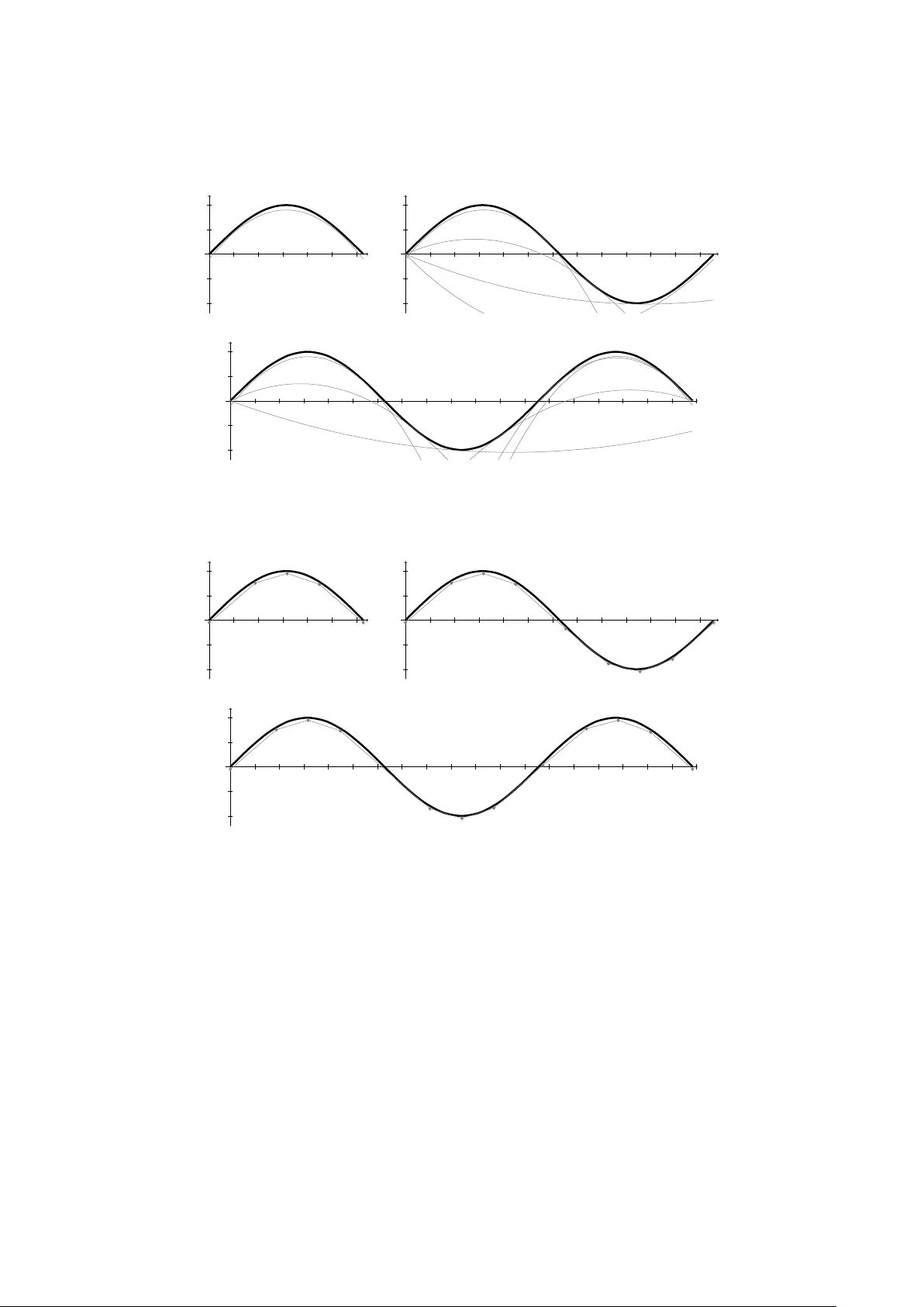
Clash of MINLP Relaxa tions: Piecewise Linear vs. Global P arabolic Adrian Gö β Abstract. Solving mixed-integer nonlinear programs (MINLPs) t ypically relies on constructing relaxations that are easier to tackle than the original problem. Recently , global parab olic (P ARA) relaxations were in tro duced, featuring separable quadratic functions – parab oloids – as global under- or ov erestimators of general nonlinear constraint functions. So far, the parab oloids are all computed at once by solving a mixed-integer linear program (MIP). F or small tolerances or wide function domains, the corresponding MIP grows in size and is even tually intractable, preven ting a meaningful comparison with established relaxation techniques. W e therefore prop ose a nov el iterative metho d to compute P ARA approxi- mations that succeeds on all tolerance-domain combinations where the original one has failed. The computational study is preceded by a thorough theoretical explanation and analysis. Finally , the improv ed metho d enables a computa- tional comparison with piecewise linear (PWL) relaxations in terms of runtime on general MINLP instances. The results show that the modern solver SCIP can solve PWL relaxations faster when the tolerance is high, shifting strongly in fav or of P ARA for tighter tolerances. W e attribute the eﬀect to the diﬀerence in the corresp onding prob- lem size: PWL relaxations introduce binary v ariables to identify the active linear piece and their n umber grows with decreasing tolerance. P ARA, on the other hand, do es not require additional v ariables such that the dimension is maintained. F or problems with at least one (co)sine constraint, the eﬀect signiﬁcantly ampliﬁes. Thereby , for medium tolerances, P ARA relaxations out- perform SCIP stand-alone. Applied problems like alternating current optimal power ﬂow (AC-OPF) feature such constraint types, leaving P ARA a viable relaxation strategy . 1. Intr oduction The mo deling p o w er of mixed-in teger nonlinear programming ( MINLP ) is undis- puted. The combination of integral comp onen ts and nonlinear in terconnection allows for the resemblance of a great v ariety of applications. These range from gas netw ork con trol [ 30 ] o ver chemical pro cesses [ 2 ] up to the design of water net works [ 8 ]. Along with this p o wer comes a certain (computational) cost, whic h makes it hard to solve general mixed-integer nonlinear programs ( MINLPs ) at scale and necessitates a retreat to simpliﬁed models, at least as an in termediate step. F or instance, in mo dern optimization softw are for MINLP lik e BARON [ 37 ], COUENNE [ 6 ], Gurobi [ 27 ], SCIP [ 28 ], or XPRESS [ 22 ] relaxations of the original problem are constructed and then solved. (A. Gö β ) University of Technology Nuremberg, Anal ytics & Optimiza tion, Dr.- Luise-Herzberg-Str. 4, 90461 Nuremberg, Germany E-mail address : adrian.goess@utn.de . Date : March 18, 2026. 2010 Mathematics Subje ct Classiﬁc ation. 90C11, 90C20, 90C26, 90C30. Key wor ds and phr ases. Mixed-in teger Nonlinear Programming, Relaxations, Mixed-Integer Linear Programming, Mixed-Integer Quadratically-Constrained Programming. 1 2 A. GÖ β A p opular tec hnique to construct relaxations of problems with general nonlinear constrain ts is their piecewise handling. With the adv ances in mixed-integer linear programming ( MIP ) throughout the last decades, constructing relaxations based on linear functions app ears as a p otentially successful option. In fact, piecewise linear ( PWL ) relaxations ha ve b een originally in tro duced in [ 31 ] – to the best of our knowledge – and are further dev elop ed and adjusted every since, e.g., see [ 3 , 12 , 16 , 29 , 36 ]. Also refer to [ 41 ] for an extensive surv ey and to [ 9 ] for a recent computational comparison. As fas as we are aw are, all of the aforementioned solvers include such relaxations. There also exist piecewise tec hniques beyond the linear realm. F or instance, the SC- MINLP approac h [ 18 , 20 ] can b e seen as an extension of PWL . F or a nonlinear and t wice con tinuously d iﬀeren tiable function f , it divides the function domain into interv als on which f is either conv ex or concav e, resp ectively . Then, the concav e parts are relaxed by PWL , whereas the conv ex parts remain. This renders the resulting relaxed problem a conv ex MINLP , which is considered (more) tractable. Even more general approaches feature piecewise quadratic [ 40 ] or piece- wise p olynomial appro ximates [ 17 ]. The resulting problems fall in to the class of mixed-in teger quadratically-constrained programming ( MIQCP ), at least after re- form ulation. Though MIQCP is still a sub class of MINLP , there exist tailored approac hes to solve such problems [ 3 , 4 , 10 , 11 , 21 , 33 , 34 , 42 ]. All those piecewise approac hes hav e the b eneﬁt to construct relaxations that can fulﬁll a prespeciﬁed tolerance. That is, giv en a tolerance ε > 0 , one can compute approximates, i.e., pieces of linear/quadratic functions, that fulﬁll the ε -accuracy with resp ect to the original problem. Thus any solution to the relaxed problem constitutes an ε -appro ximate solution which often suﬃce in practice. As an additional adv antage, the c haracter of the relaxed problem as a MIP or MIQCP problem allows to lev erage tailored solvers. Naturally , those b eneﬁts are not without cost. Depending on the modeling tec hnique, they come with the introduction of binary v ariables whose num ber gro ws with the num ber of pieces. The approximates – e.g., linear pieces – lack a global v alidity , i.e., they do not constitute global under-/o verestimators of the constrain t function, and thus need to b e “disabled” outside their corresp onding in terv al. Hence, the resulting relaxation gro ws in (v ariable) size, whic h may imp ose computational challenges for large problems or tigh t tolerances. In a ﬁrst attempt to circum ven t additional integer v ariables, the authors of [ 26 ] introduced a framew ork to compute global parab olic ( P ARA ) approximations of functions. The approximates are p ar ab oloids , i.e., separable quadratic functions, globally under-/ov erestimating a constrain t function. Although not necessarily b eing conv ex, the global v alidity allows to incorp orate the parab oloids as constraints without the necessit y of additional binary v ariables. That is, the problem size grows in the n umber of constrain ts only , but some solv ers lik e SCIP seem to handle those similar-shap ed constraints quite w ell, compare [ 26 ]. Although the P ARA approac h seems to b e a viable relaxation technique, the metho d to compute resp ectiv e P ARA appro ximations in [ 26 ] is computationally limited. It computes all approximating parab oloids at once b y rep etitiv ely solving MIP problems. Thereby , their size grows with domain width and decreasing tolerance, lea ving them even tually not solv able under limited resources. Consequently , [ 26 ] rep orts v alid parab olic approximations only on artiﬁcial domains and with resp ect to mo derate tolerances, preven ting a meaningful comparison with established techniques lik e PWL. W e thus introduce a nov el iterative metho d that leverages diﬀerentiabilit y of the constrain t functions in combination with a factorable problem structure to compute MINLP RELAXA TIONS: PIECEWISE LINEAR VS. GLOBAL P ARABOLIC 3 P ARA appro ximations for tight tolerances and wide domains. In Section 3 , we in tro duce our metho d formally , give pro of of its correctness, and show case that it is indeed able to succeed on tolerance-domain com binations that are left as unsolved b y the approach in [ 26 ]. F urthermore, our method then allows for a comparison against PWL relaxations in terms of n umbers of appro ximates – linear pieces versus parab olas – (Section 3.2.2 ) and computational eﬃcacy (Section 4 ). The remainder is dedicated to establish common ground in Section 2 by a presen tation of the notation and the optimization problem. F urther, it gives a short in tro duction into PWL (Section 2.3 ) and the original P ARA approac h (Section 2.4 ). W e close the article with some concluding remarks in Section 5 . Pro ofs and additional results can b e found in App endix A and Appendix B , respectively . 2. Preliminaries Before diving into the main topic of the article, we wan t to clarify notation and state the problem(s) in question. During later statements and pro ofs this will foster clarity . Additionally , w e aim to explain basic concepts such as the relaxation tec hniques. 2.1. Notation. Consider the naturals without zero N = { 1 , 2 , 3 , . . . } . W e will use n ′ , n ∈ N as the original v ariable dimension and the v ariable dimension after reform ulation, respectively , and m ′ , m ∈ N as the num b er of original constrain ts and constrain ts of interest, respectively . F or counting or n um b ering v ariables, constrain ts, or other ob jects, we introduce the short notation [ n ] : = { 1 , 2 , . . . , n } . V ectors are giv en in b old suc h as x ∈ R n , whereas components are italicized, e.g., x = ( x 1 , . . . , x n ) ⊤ . F or an interv al D = [ x, x ] , we denote its length by |D | : = | x − x | , using D  = ∅ and |D | > 0 interc hangeably . The in terior is denoted by in t ( D ) = ( x, x ) . 2.2. Mathematical Problem. W e consider general MINLP problems of the form min x ′ ∈ R n ′ c ( x ′ ) s.t. g j ( x ′ ) ≤ 0 , j ∈ [ m ′ ] , x ′ i ∈ Z , i ∈ I , x ′ ∈ [ x ′ , x ′ ] , (P gen ) where I ⊆ [ n ′ ] . The v ectors x ′ and x ′ denote comp onen t-wise b ounds to x ′ , which w e assume to b e ﬁnite. Note that this kind of formulation is no restriction, i.e., it do es include equality constraints by re-mo deling g ( x ′ ) = 0 to g ( x ′ ) ≤ 0 and − g ( x ′ ) ≤ 0 . The inv olved functions are assumed to b e suﬃcien tly smo oth, which is common in MINLP , see, e.g., [ 19 ]. That is, we assume them to b e once con tinuously diﬀeren tiable and, if necessary , to b e able to compute their optimum ov er any compact domain. Dep ending on the particular metho d the latter can require t wice con tinuous diﬀerentiabilit y . W e also assume the inv olved functions to b e factor able , see, e.g., [ 5 , 32 ]. That is, they are comp osed of ﬁnitely many binary op erations (sum, pro duct, division, p o wer) and ﬁnitely many unary op erations ( sin , cos , exp , log , |·| ) of constants and v ariables. Equiv alently , factorable functions can b e expressed in terms of an expression tree whic h has the mentioned op erations as nodes as w ell as v ariables and constants as lea ves. F or a given non-leaf no de N , the child no de(s) represents the argument(s) of the op eration in N . More detailed explanations can b e found in [ 5 , 14 , 25 , 35 , 38 ]. Nearly all instances from MINLPLib [ 13 ] are av ailable in the OSiL ﬁle format [ 23 ], whic h directly provides the expression tree structure. 4 A. GÖ β The factorability allows to rewrite the original problem formulation in terms of biv ariate pro ducts and one-dimensional functions by in tro duction of auxiliary v ariables in place of intermediate no des. F or example, consider g ( x ′ ) = sin ( x ′ 1 x ′ 2 ) 2 . By in tro duction of v ariables ˜ x and y w e can rewrite the constraint g ( x ′ ) ≤ 0 to y 2 ≤ 0 , y = sin ( ˜ x ) , and ˜ x = x ′ 1 x ′ 2 . Note that ﬁnite b ounds on x ′ can be propagated to ˜ x and y . F or instance, x ′ 1 ∈ [1 , 2] and x ′ 2 ∈ [0 , π / 4] result in ˜ x ∈ [0 , π / 2] and y ∈ [0 , 1] . Those reformulations, as p erformed by the mo dern MINLP solv ers cited in the in tro duction, allow us to fo cus on one-dimensional, general nonlinear constrain t functions only . F or this purp ose, we denote them after reformulation as f j , e.g., f 1 ( ˜ x ) = sin ( ˜ x ) , and collect all linear and quadratic constraints (including b ounds) as well as integralit y restrictions in a set Ω . F urthermore, vector x represents a concatenation of x ′ − and newly introduced ˜ x -v ariables, whereas the y -v ariables are k ept for clarity . In conclusion, we assume our problem at hand to b e presen ted as min ( x , y ) ∈ R n × R m c ( x ) s.t. f j ( x i j ) ≤ y j , j ∈ [ m ] , ( x , y ) ∈ Ω . (P) The n umber of x -v ariables is no w denoted b y n , whereas m is the n umber of “in teresting” constraints and y -v ariables. The subindex j of i j indicates that a v ariable x i ma y o ccur in sev eral constrain ts j . Note that the constraint functions f j are only deﬁned on a one-dimensional and ﬁnite domain, but remain general nonlinear ones. Therefore, despite any reform ulation, it cannot b e exp ected to compute an exact solution to ( P ). Instead, in practice the user sp eciﬁes an approximation tolerance ε > 0 and is satisﬁed when obtaining an ε -appro ximate solution, i.e., a p oint that violates the nonlinear constrain ts by a v alue of at most ε . Such a point is equiv alen t to an exact optimal solution of the problem min c ( x ) s.t. f j ( x i j ) ≤ y j + ε, j ∈ [ m ] , ( x , y ) ∈ Ω . (P ε ) F or computing an ε -appro ximate solution, a natural idea is to substitute f j in ( P ) b y an ε -relaxation ˆ f j , i.e., it holds that f j − ˆ f j ≤ ε on the domain of f j . The resulting relaxed problem reads min c ( x ) s.t. ˆ f j ( x i j ) ≤ y j , j ∈ [ m ] , ( x , y ) ∈ Ω . (P rel ) A solution ( x ⋆ , y ⋆ ) for ( P rel ) then fulﬁlls f j ( x ⋆ i j ) ≤ ˆ f j ( x ⋆ i j ) + ε ≤ y ⋆ j + ε for j ∈ [ m ] and is thus a v alid ε -approximate solution. A strategy for computing a linear ˆ f j , which has reattained recent attention, is the approac h b y piecewise linear functions. In the follo wing, w e pro vide an introduction of it. 2.3. Piecewise Linear Mo del. W e consider a nonlinear function f and a ﬁnite domain D = [ x, x ] suc h that x < x . First, we will explain the computation and mo deling of a piecewise linear ( PWL ) appr oximation , b efore extending it to a PWL r elaxation . A PWL appro ximation ¯ f of f can b e constructed as a linear int erp olation of f and is thus deﬁned b y breakp oints { t 0 , t 1 , . . . , t K } with t 0 = x , t K = x , and MINLP RELAXA TIONS: PIECEWISE LINEAR VS. GLOBAL P ARABOLIC 5 t k − 1 < t k for k ∈ [ K ] . Parameter K ∈ N denotes the num b er of interv als/linear pieces. Then, for x ∈ [ t k − 1 , t k ] , it is ¯ f ( x ) = f ( t k − 1 ) t k − x t k − t k − 1 + f ( t k ) x − t k − 1 t k − t k − 1 . Giv en an approximation tolerance ε > 0 , we describ e one w ay to compute ¯ f . Starting with K = 1 , t 0 = x , t 1 = x , w e chec k the condition | ¯ f ( x ) − f ( x ) | ≤ ε for all x ∈ [ t 0 , t 1 ] . Since suc h a chec k can b e p erformed by computing the maxim um/minimum of the diﬀerence, the aforementioned suﬃcient diﬀerentiabilit y comes into play . If the condition is met, ¯ f is a v alid ε -appro ximation of f . Otherwise, w e execute a binary search for the largest t 1 to fulﬁll the condition. After t 1 is determined, we increment K and start to ﬁnd the largest t 2 suc h that the condition is met on [ t 1 , t 2 ] . The pro cedure is iterated and stops when t K = x . W e refer to [ 9 ] for a current implementation. Besides its computation, the more imp ortan t aspect is the incorp oration of a PWL appro ximation ¯ f in to an optimization mo del. T o the b est of our knowledge, a PWL form ulation was ﬁrst introduced in [ 31 ]. The metho d explained there is referred to as incr emental metho d or δ -metho d . In the mean time, there hav e b een established several adjusted form ulations, see [ 3 , 12 , 16 , 29 , 36 ], that try to improv e computational p erformance, e.g., by reducing the num ber of v ariables in the mo del. Recen tly though, Braun and Burlacu [ 9 ] demonstrated that in some settings the incremen tal metho d is still sup erior to all other metho ds in terms of computational p erformance. Therefore, we choose it for our computational comparison later on and explain it in the follo wing, rephrasing mainly from [ 9 ]. F or a giv en x ∈ D , we ﬁrst need to determine the corresp onding in terv al index ¯ k ∈ [ K ] such that x ∈ [ t ¯ k − 1 , t ¯ k ] . In the incremental metho d, we in tro duce one binary v ariable u k for each but the last in terv al [ t k − 1 , t k ] , k ∈ [ K − 1] , and aim to ha ve u k = 1 for all interv als with t k ≤ x , else u k = 0 . In other terms, the binary v ariable u k is activ ated whenev er x exceeds the upp er b ound of the corresp onding k th interv al until the in terv al containing x is reached. F ormally , this can b e ensured b y t 0 + K − 1 X k =1 u k ( t k − t k − 1 ) ≤ x, u k +1 ≤ u k , for k ∈ [ K − 1] . Besides determining the relev an t in terv al [ t ¯ k − 1 , t ¯ k ] , we second need to compute the relativ e distance of x inside it. Here, the incremental metho d advocates to introduce con tinuous v ariables δ k ∈ [0 , 1] corresp onding to the interv als, k ∈ [ K ] . As for the binary v ariables u k , the con tinuous ones δ k are also set to one when x exceeds t k , whic h is enforced by the inequalities δ k +1 ≤ u k , for k ∈ [ K − 1] . (1) The contin uous v ariables even allow to mo del the v alue of x explicitly as x = t 0 + K X k =1 δ k ( t k − t k − 1 ) , (2) whereas for the in terp olation v alue w of f , we get w = f ( t 0 ) + K X k =1 δ k ( f ( t k ) − f ( t k − 1 )) . (3) 6 A. GÖ β In conclusion, the incremental metho d p oses a model for PWL appro ximation of the form ( 1 ) , ( 2 ) , ( 3 ) , δ 1 ≤ 1 , u k ≤ δ k , k ∈ [ K − 1] , δ K ≥ 0 , u k ∈ { 0 , 1 } , k ∈ [ K − 1] , (4) where the edge cases are resp ected as well. Note that the binary v ariables are necessary to ﬁx the δ -v ariables to their resp ectiv e b ounds such that only the relev an t one is p oten tially fractional. Since this main ingredient of “ﬁlling” or “incrementation” is often mo deled via v ariables named δ , the metho d is also known b y this resp ective name. Note that system ( 4 ) mo dels a PWL appr oximation of f suc h that | w − f | ≤ ε on D . Thus, a simply replacement of eac h f j in ( P ) with a corresp onding w j and ( 4 ) do es in general not p ose a relaxation ( P rel ), but an appro ximated problem. Consequen tly , if the approximated problem is solved, its solution is not guaranteed to b e also a solution of ( P ε ). How ev er, to retrieve a relaxation, we can deﬁne ε ′ : = ε/ 2 , compute a PWL appro ximation with resp ect to ε ′ , and shift the result for ε/ 2 . In particular, the PWL appro ximation then ensures that | w − f ( x ) | ≤ ε ′ for all x ∈ D . This implies that w − ε ′ ≤ f ( x ) and thus | ( w − ε ′ ) − f ( x ) | ≤ | w − f ( x ) | + ε ′ ≤ 2 ε ′ = ε . In other terms, a shift of the function v alues f ( t k ) in ( 3 ) by ε ′ is a shift in w and results in a underestimation – th us relaxation like ( P rel ) – satisfying a tolerance of ε . Such a pro cedure for obtaining a PWL relaxation is p erformed throughout the presen t article and we refer to this relaxation technique simply b y PWL. 2.4. Global One-sided Parabolic Mo del. The recently introduced approach of global one-sided parabolic (P ARA) appro ximations and relaxations [ 26 ] aims to circum ven t the use of binary v ariables as in PWL . F or a given constraint function f , it computes an appro ximation ˘ f as the p oin t-wise maximum of parab oloids, i.e., separable univ ariate quadratic functions, that underestimate f on D individually and satisfy the given appro ximation tolerance. As we consider one dimensional constraint functions f only , we refer to this t yp e of appro ximates as parab olas. F ormally , for a set of K ∈ N parab olas { p k } k ∈ [ K ] , the approximation is ˘ f ( x ) = max k ∈ [ K ] p k ( x ) suc h that f − ε ≤ ˘ f ≤ f on D . (5) In other terms, ˘ f represen ts an epigraph approximation of f . Due to the global underestimation, we can simply replace each constraint in ( P ) by a corresp onding parab olic approximation and end up with ( P rel ). T aking the presen tation as ‘ ≤ ’- constrain ts and the p oin t wise maxim um in to accoun t, it even simpliﬁes to the set of constraints p k ( x ) ≤ y , k ∈ [ K ] . This makes the mo deling of P ARA relaxations straigh tforward and does not rely on the use of binary v ariables. It remains to clarify the computation of p k in [ 26 ]. F or a constraint function f and its domain D = [ x, x ] , the approach requires a global Lipschitz constant L > 0 of f . This can b e considered a weak er assumption in comparison to contin uous diﬀeren tiability , since maximizing | f ′ | on D giv es L . Based on the magnitude of L , the approach in [ 26 ] p erforms a binary searc h on the n umber of parab olas K . During one search iteration, K is ﬁxed and a MIP problem is constructed in which the co eﬃcien ts of the parab olas are considered as v ariables. The problem’s constraints ensure the ε -appro ximation prop ert y of a solution, whereas the ob jective controls the global underestimation, i.e., the ﬁrst and second inequality in ( 5 ), resp ectiv ely . If the MIP problem is solved in a given time limit with ob jective of zero, the corresp onding MINLP RELAXA TIONS: PIECEWISE LINEAR VS. GLOBAL P ARABOLIC 7 parab olas fulﬁll ( 5 ) and the current K is decreased. Otherwise, the n umber of parab olas K is increased. The weak assumptions necessary for the approac h represen t a clear adv antage, as it lea ves it applicable for a really broad class of constraint functions. How ever, relying on the solution of several MIP problems can b e computationally challenging and results in function-domain- ε com binations that are not computable, see the comparison b elow in Section 3.2 for more details. In fact, the article [ 26 ] in tro duces a theoretically v alid as well as a more practical option of this approac h. The latter circum ven ts some of the challenges by relaxing particular constraints of the MIP and by incorp orating manual chec ks. Those c hanges turn it in to a computationally more eﬃcient version. Hence, we conduct the later comparison in Section 3.2 with resp ect to this version and refer to it as practical-MIP , following the original source. 3. Computing P arabolas F ast Inspired by the computation of PWL appro ximations, w e introduce a nov el metho d to compute P ARA appro ximations for general nonlinear functions f in an iterative manner. W e recall that f is assumed to b e suﬃciently contin uous diﬀeren tiable and deﬁned on a domain D = [ x, x ] . An explanation of the metho d and resp ective pro ofs of correctness are provided in Section 3.1 . W e refer this pro cedure as the P ARA appro ximation metho d or shortly P ARA . It is indeed able to compute parab olas for cases where the original metho d from [ 26 ] has failed, see Section 3.2 . The computational p erformance even allows to conclude the present section with a comparison of num b er of approximates, i.e., parabolas and linear pieces, on general nonlinear functions that o ccur frequently in the MINLPLib [ 13 ]. 3.1. Method. In contrast to the metho d in [ 26 ], we asso ciate one parab ola p k , k ∈ [ K ] , with a certain domain D k : = [ t k − 1 , t k ] , on whic h it fulﬁlls the ε - appro ximation, i.e., f ( x ) − ε ≤ p k ( x ) , for all x ∈ D k . (6) T o construct a global ε -appro ximation with all parab olas, they m ust satisfy the ﬁrst inequalit y in ( 5 ) and w e th us require [ k ∈ [ K ] D k = D . (7) Sim ultaneously , as describ ed ab o v e, each p k is supp osed to serve as a global under- estimator of f , i.e., p k ( x ) ≤ f ( x ) , for all x ∈ D . (8) This settles the description of the requirements. Our new approach returns the parabolas “from left to righ t”, i.e., it computes a parab ola which satisﬁes prop ert y ( 6 ) on [ x, t 1 ] = [ t 0 , t 1 ] , and then pro ceeds to [ t 1 , t 2 ] un til it reaches the upp er b ound x with the ﬁnal interv al [ t K − 1 , t K ] = [ t K − 1 , x ] . Here, K ≥ 0 indicates the necessary num ber of parab olas, which is determined a-p osteriori. Such a pro cedure can b e leveraged for computing PWL appro ximations as well, see Section 2.3 . Let’s turn to a particular iteration k and inv estigate the challenge at hand. The curren t lo wer b ound is ﬁxed at t k − 1 < x . T o cov er a large interv al, on whic h p k is a v alid ε -appro ximation, we aim to maximize the next upp er b ound t k ≤ x . Enforcing ( 6 ) and ( 8 ), we can formulate this as the semi-inﬁnite optimization 8 A. GÖ β problem max t k , ˜ a, ˜ b, ˜ c t k s.t. ˜ ax 2 + ˜ bx + ˜ c ≥ f ( x ) − ε, for all x ∈ [ t k − 1 , t k ] = D k , (9a) ˜ ax 2 + ˜ bx + ˜ c ≤ f ( x ) , for all x ∈ D , (9b) where we deﬁne t 0 = x for D 1 and ( ˜ a, ˜ b, ˜ c ) denote v ariables for the co eﬃcien ts of p k . A solution ( a k , b k , c k ) to this problem then gives p k ( x ) : = a k x 2 + b k x + c k , satisfying ( 6 ) and ( 8 ) by ( 9a ) and ( 9b ), respectively . How ev er, the constraints ( 9 ) are inﬁnitely many and thus require further treatment. In a ﬁrst attempt let us assume to hav e a ﬁxed parabola p k and a ﬁxed upp er b ound t k . Then, computing max x ∈D p k ( x ) − f ( x ) = max x ∈D a k x 2 + b k x + c k − f ( x ) , (10) and max x ∈D k f ( x ) − p k ( x ) = max x ∈D k f ( x ) − ( a k x 2 + b k x + c k ) , (11) can b e considered computational tractable, since b oth problems require to maximize diﬀerences of contin uously diﬀeren tiable functions on a closed interv al. This can b e conducted by means of Newton-type metho ds, for instance. Let z k and z ε k denote the solutions for ( 10 ) and ( 11 ), resp ectiv ely . Then, ( 9a ) is fulﬁlled if and only if f ( z ε k ) − p k ( z ε k ) ≤ ε , and, analogously , ( 9b ) is fulﬁlled if and only if p k ( z k ) − f ( z k ) ≤ 0 . In the case that at least one of these inequalities do es not hold, a decrease of the interv al length |D k | , th us a shift of t k to wards t k − 1 , and a new computation of p k ma y resolv e the issue. Based on this observ ation, w e propose a t wo-step or inner-outer approach. Let k b e the current iteration index, then • an outer loop tries to compute a maximal upp er b ound t k for the curren t in terv al [ t k − 1 , t k ] , but iteratively reduces the v alue of t k if the inner lo op fails, shifting t k in the direction of t k − 1 , and • an inner lo op aims to ﬁnd a feasible set of co eﬃcien ts ( a k , b k , c k ) , deﬁning the current parab ola p k suc h that ( 9 ) hold true. 3.1.1. Inner L o op. W e start our explanation with the inner loop. F or ease of notation, we drop the iteration index k and thus write the curren t (lo cal) domain D k = D loc = [ t, t ] as well as p k ( x ) = p ( x ) = ax 2 + bx + c . Throughout the inner lo op, we force p to cross f − ε at the bounds of D loc . In particular, this can be expressed as p ( t ) = f ( t ) − ε, p ( t ) = f ( t ) − ε, whic h reads in explicit form as at 2 + bt + c = f ( t ) − ε, (12a) at 2 + bt + c = f ( t ) − ε. (12b) Neglecting ( 9b ) for the moment, the in tuition b ehind this measure is as follows: If the parab ola p fulﬁlls ( 9a ) and simultaneously p ( t ) > f ( t ) − ε or p ( t ) > f ( t ) − ε , the domain D loc could hav e been chosen larger. Fixing p at the b ounds of D loc reduces to original degrees of freedom when determining the three co eﬃcien ts of p b y tw o. In other words, giv en one of the MINLP RELAXA TIONS: PIECEWISE LINEAR VS. GLOBAL P ARABOLIC 9 co eﬃcien ts a , b , or c , this system uniquely determines the remaining tw o. T o see this, assume co eﬃcien t a as ﬁxed and rewrite the system ( 12 ) to A v = d , where A =  t 1 t 1  , d =  f ( t ) − ε − at 2 f ( t ) − ε − at 2  , and v =  b c  ⊤ . When D loc  = ∅ , so t < t , it holds det ( A ) = t − t < 0 and the system alwa ys attains a unique solution. Instead of ﬁxing co eﬃcien t a to determine ( b, c ) , we combine ( 12 ) with ( 9 ) and can derive b ounds to the quadratic co eﬃcient a . This will allow to determine the existence of a feasible set of co eﬃcien ts ( a, b, c ) and constitute the main ingredient of the inner loop. In the following, the deriv ation of b ounds is formalized. Lemma 1 (Bounds on a ) . L et f : D → R b e as ab ove and in t ( D )  = ∅ . F urther, let ε > 0 and D lo c : = [ t, t ] ⊂ D such that x < t < t < x , implying in t ( D lo c )  = ∅ . F or a p ar ab ola p ( x ) = ax 2 + bx + c , assume ( 12 ) . Then the fol lowing implic ations hold true. (a) Consider b x ∈ D \ D lo c . Then p ( b x ) ≤ f ( b x ) if and only if a ≤ f ( b x ) − f ( t ) + ε ( b x − t )( b x − t ) − f ( t ) − f ( t ) ( t − t )( b x − t ) = : A ( b x ) . (b) Consider b x ∈ in t( D lo c ) . Then p ( b x ) ≤ f ( b x ) if and only if a ≥ f ( b x ) − f ( t ) + ε ( b x − t )( b x − t ) − f ( t ) − f ( t ) ( t − t )( b x − t ) = : A ( b x ) . (c) Consider b x ∈ in t( D lo c ) . Then p ( b x ) ≥ f ( b x ) − ε if and only if a ≤ f ( b x ) − f ( t ) ( b x − t )( b x − t ) − f ( t ) − f ( t ) ( t − t )( b x − t ) = : B ( b x ) . Pr o of. As a preparatory step, we subtract ( 12a ) from ( 12b ) and get a ( t 2 − t 2 ) + b ( t − t ) = f ( t ) − f ( t ) , whic h is equiv alent to a ( t + t ) + b = f ( t ) − f ( t ) t − t (13) b y division with ( t − t ) . This preliminary work will supp ort the pro of for every of the three cases. Case (a). Starting oﬀ, we write the condition from (a) explicitly , i.e., a b x 2 + b b x + c ≤ f ( b x ) . By subtracting ( 12a ), this is equiv alen t to a ( b x 2 − t 2 ) + b ( b x − t ) ≤ f ( b x ) − f ( t ) + ε. No w, rearranging ( 13 ) for b and plugging the result into the former gives a ( b x 2 − t 2 ) +  f ( t ) − f ( t ) t − t − a ( t + t )  ( b x − t ) ≤ f ( b x ) − f ( t ) + ε ⇐ ⇒ a  b x 2 − t 2 − t b x − t b x + tt + t 2  ≤ f ( b x ) − f ( t ) + ε − f ( t ) − f ( t ) t − t ( b x − t ) ⇐ ⇒ a ( b x − t )( b x − t ) ≤ f ( b x ) − f ( t ) + ε − f ( t ) − f ( t ) t − t ( b x − t ) . As b x ∈ D \ D loc , either b x < t < t or t < t < b x . That is, ( b x − t )( b x − t ) > 0 and thus division by this term do es not change the direction of the inequalit y but leads to (a). 10 A. GÖ β Case (b). This is analogous to case (a), how ever, the last division c hanges the sign of the inequality , as b x ∈ int( D loc ) and thus ( b x − t )( b x − t ) < 0 . Case (c). Again, w e write the condition from (c) explicitly and get a b x 2 + b b x + c ≥ f ( b x ) − ε. Subtraction of ( 12a ) gives a ( b x 2 − t 2 ) + b ( b x − t ) ≥ f ( b x ) − f ( t ) . F ollo wing the strategy from previous cases and resp ecting that b x ∈ int ( D loc ) gives the desired inequality . □ Lemma 1 implies that every point in D \ D loc implicitly gives an upp er b ound to the quadratic co eﬃcien t a and ev ery point inside D loc ev en im- plies lo wer and upp er b ounds to a . Setting a ← sup x ∈ int( D loc ) A ( x ) and a ← min  inf x ∈D\D loc A ( x ) , inf x ∈D loc B ( x )  , we ensure the existence of a feasible co eﬃcien t a (th us parab ola) if and only if a ≤ a . A feasible a can then b e comple ted computing ( b, c ) by solving the linear system ( 12 ). In turn, if w e kno w that a > a , there exists no feasible a and we need to shrink D loc in the outer loop. The computation of the minima and maxima ab o v e to determine a and a is non-trivial, since the v ariable x app ears in the denominator of a fraction, esp ecially in a term that conv erges to inﬁnit y . Hence, we compute these b ounds iteratively , starting with some initial v alues a 0 and a 0 . In fact, as any a ∈ [ a, a ] is v alid, we initialize a 0 with negative inﬁnity and alwa ys set a to b e the current upp er b ound. This will facilitate the presentation of the metho d and showing its correctness. Ho wev er, it remains to ﬁnd a v alue for a 0 , which can also be derived by the results of Lemma 1 as mentioned b elo w. Remark 2. Consider a p oint x ∈ int ( D lo c ) and L emma 1 (c). If x → t , the ine quality b ounding c o eﬃcient a turns into a ≤ f ′ ( t ) t − t + f ( t ) − f ( t ) ( t − t ) 2 = ( f ( t ) − f ( t ) + ( t − t ) f ′ ( t )) / ( t − t ) 2 . This dir e ctly gives an upp er b ound to a , which c an b e use d for a 0 . F or the c ase x → t , we ﬁrst ne e d to r ewrite B ( x ) . By r esp e cting that D : = 1 ( x − t )( x − t ) − 1 ( t − t )( x − t ) = − 1 ( t − t )( x − t ) , we c an derive that B ( x ) = f ( x ) − f ( t ) − f ( t ) + f ( t ) ( x − t )( x − t ) − f ( t ) − f ( t ) ( t − t )( x − t ) = f ( x ) − f ( t ) ( x − t )( x − t ) + ( f ( t ) − f ( t )) D = f ( x ) − f ( t ) ( x − t )( x − t ) − f ( t ) − f ( t ) ( y − t )( x − t ) . Then, c onsidering x → t for x ∈ int( D lo c ) , L emma 1 (c) pr ovides that a ≤ ( f ( t ) − f ( t ) + ( t − t ) f ′ ( t )) / ( t − t ) 2 . T aking the minimum of b oth those upp er b ounds, le ads to a 0 for our inner lo op. After initializing the quadratic co eﬃcien t a , the remaining coeﬃcients ( b, c ) can b e computed by solving ( 12 ). Then, the inner lo op tests for ( 6 ) and ( 8 ) by MINLP RELAXA TIONS: PIECEWISE LINEAR VS. GLOBAL P ARABOLIC 11 computing ( 10 ) on D \ D loc and D loc separately , as well as ( 11 ) on D loc . Explicitly , for a ﬁxed parabola p , this is max x ∈D\D loc p ( x ) − f ( x ) , (14a) max x ∈ int( D loc ) p ( x ) − f ( x ) , (14b) max x ∈ int( D loc ) f ( x ) − p ( x ) − ε. (14c) W e denote the solutions by x 1 , x 2 , x 3 and their v alues by v 1 , v 2 , v 3 , resp ectively . If v max : = max { v 1 , v 2 , v 3 } exceeds the threshold of zero, the current choice of co eﬃcien t a is infeasible and x 1 , x 2 , x 3 are considered as candidates for “ b x ” in Lemma 1 , implying an up date of the current b ounds a l and a l on a . The pro cess is iterated until the b ounds are contradictory , signaling the absence of a feasible triple ( a, b, c ) , or until the constrain ts ( 9 ) are satisﬁed. This process is summarized in Metho d 1 . Arro ws are alwa ys p oin ting to wards the ob ject that is returned by this step. Metho d 1 Inner lo op – Computing ( a, b, c ) . Input: (Lo cal) Interv al b ounds t and t such that t < t . Output: Co eﬃcien ts ( a, b, c ) deﬁning p satisfying ( 9 ) or “Infeasible”. 1: Initialize a 0 according to Remark 2 , a 0 ← −∞ , and l ← 0 . 2: Set a 0 ← a l and compute ( b l , c l ) according to ( 12 ). 3: while a l ≤ a l do 4: Compute ( 14 ) → x 1 , x 2 , x 3 , v max . 5: if v max ≤ 0 then 6: return ( a l , b l , c l ) . 7: end if 8: Up date a l +1 and a l +1 with x 1 , x 2 , x 3 according to Lemma 1 . 9: Incremen t l ← l + 1 . 10: Set a l ← a l and compute ( b l , c l ) according to ( 12 ). 11: end while 12: return “Infeasible”. After its presentation, we contin ue b y formally showing the correct mo de of op eration of the inner loop. Theorem 3 (Correctness of Metho d 1 ) . If ther e exists a solution ( a, b, c ) fulﬁl ling ( 9 ) and ( 12 ) , Metho d 1 r eturns one or c onver ges to it. Otherwise, it r eturns that ther e is no such solution. The following provides a pro of sketc h, for which the details can b e found in App endix A.1 . Pr o of. By leveraging Lemma 1 the existence of ﬁnite b ounds a ≤ a is equiv alent to the existence of a solution ( a, b, c ) . This represen ts the main ingredient. If there exists a solution, the condition of the while-lo op is alwa ys met. Since a l in iteration l is c hosen to be the current a l , also a l ≥ a for all l . By Lemma 1 , it th us alwa ys holds that p ≤ f on in t ( D loc ) . The remaining cases, p ≤ f on D \ D loc and p ≥ f − ε on in t ( D loc ) , are pro ven following the same strategy: W e use ( 12 ) to write down a parameterized v ersion of parab ola p in the quadratic co eﬃcient a . This allows us to show conv ergence by contradiction. □ 12 A. GÖ β 3.1.2. Outer L o op. While the inner loop computes an appro ximating parab ola for a given interv al or asserts with its imp ossibilit y , it remains to consider the in terv al b ounds. W e prop ose to start with the global in terv al [ t 0 , t 1 ] : = [ x, x ] and consecutiv ely shift t 1 to ward t 0 , un til a suitable parab ola can b e computed by the inner lo op. After storing the parab ola and the asso ciated domain [ t 0 , t 1 ] , the remaining interv al [ t 1 , x ] is considered next. This is iterated until K parab olas p k with their asso ciated domains D k are computed, cov ering the entire global domain D , i.e., fulﬁlling ( 7 ). This pro cedure is presented in pseudoco de in Metho d 2 . Metho d 2 Outer lo op – Computing D k Input: (Global) Domain D = [ x, x ]  = ∅ , approximation tolerance ε > 0 . Output: A set of co eﬃcien ts ( a k , b k , c k ) deﬁning p k , k ∈ [ K ] , K ∈ N , suc h that ( 5 ). 1: Initialize k ← 1 , t 0 ← x , t 1 ← x . 2: while t k − 1 < x do 3: Call Metho d 1 on [ t k − 1 , t k ] → ( a, b, c ) or “Infeasible”. 4: if “Infeasible” then 5: Shift t k to wards t k − 1 . 6: else 7: Store ( a k , b k , c k ) . 8: Set t k +1 ← x and increment k ← k + 1 . 9: end if 10: end while 11: return Parameters ( a k , b k , c k ) for k ∈ [ k ] . Dep ending on the t yp e of shift applied in Step 5 , the n umber of parab olas and th us iterations v aries. W e wan t to brieﬂy discuss this eﬀect b y supp osing a shift in form of a conv ex combination, i.e., t k ← λt k − 1 + (1 − λ ) t k for λ ∈ (0 , 1) . If λ is near 1, the shift is strong to wards t k − 1 and the length of the current interv al D k is decreased rapidly . In consequence, it is likely to ﬁnd a suitable parab ola with ( 6 ) and ( 8 ) after only a couple of “Infeasible”-iterations of the inner loop. How ev er, it tak es a considerable n umber K of interv als – thus parab olas – to cov er the en tire domain, i.e., to reach ( 7 ). In turn, a v alue of λ close to 0 results in the opp osite eﬀect, p oten tially computing a small num b er of parab olas – thus few quadratic constrain ts for the P ARA relaxation – but for a certain computational cost. The speciﬁc num b er of calls of the inner lo op depends on the function f and its domain D to b e considered, as well as on the v alue of λ . F rom the theoretical side, how ever, it remains to sho w that Metho d 2 conv erges at al l . In the following, w e will demonstrate it, supp osing the shift in Step 5 to b e a true decrease of the in terv al length of D k that still ensures |D k | > 0 . In particular, we sho w that for small enough domains D k , there exists a resp ective solution p k . This allo ws to derive b y Theorem 3 that the inner lo op at least conv erges to suc h a solution. Considering n umerical precision and thus ﬁniteness of the inner lo op, we can conclude that Metho d 2 terminates. Note that we will only leverage Lipschitz con tinuit y of our function f for this pro of. As noted in Section 2.4 , a global Lipsc hitz constan t L can b e computed as (an upp er b ound to) max {| f ′ ( x ) | | x ∈ D } , i.e., the assumptions of the theorem apply to the given setup. Keeping the assumptions on f lo w, ho wev er, allows for wider application and a comparison of the pro of techniques to the ones in [ 26 ]. Theorem 4 (Correctness of Method 2 ) . L et D  = ∅ , f : D → R b e glob al ly Lipschitz c ontinuous with L > 0 and ε > 0 . Then, for any interval length ∆ > 0 with ∆ ≤ ε/ (3 L ) and |D | / ∆ ∈ N , one c an cho ose D k as a p artition of D with |D k | = ∆ MINLP RELAXA TIONS: PIECEWISE LINEAR VS. GLOBAL P ARABOLIC 13 domain D exp [ − 5 , − 2] [ − 2 , 2] [ − 5 , 2] [ 2 , 5] [ − 2 , 5] [ − 5 , 5] sin [ − π 2 , π 2 ] [ π 2 , 3 π 2 ] [ − π 2 , 3 π 2 ] [ 0 , π ] [ π , 2 π ] [ 0 , 2 π ] T able 1. F unction-domain com binations to appro ximate with Metho d 2 for comparison with [ 26 ]. and by setting a k = − 4 L/ ∆ ther e exist p ar ab olas p k ( x ) = a k x 2 + b k + c k , k ∈ [ |D | / ∆] , fulﬁl ling the pr op erties ( 6 ) and ( 8 ) . The following provides a pro of sketc h, since the full pro of is of tec hnical nature. Details can b e found in App endix A.2 . Pr o of. F or a given lo cal interv al D loc with length ∆ , we show the existence of a parab ola p such that a) p ( x ) ≥ f ( x ) − ε on D loc , b) p ( x ) ≤ f ( x ) on D loc , and c) p ( x ) ≤ f ( x ) on D \ D loc . F or case a), w e mak e use of Lemma 1 and show that ˜ a ≤ B ( x ) for all x ∈ int ( D loc ) . Cases b) and c) are straigh tforward, using the Lipsc hitz contin uit y and the assump- tions to ∆ . Denoting the mid point of D loc as ˜ t , all three cases distinguish x ≤ ˜ t and x ≥ ˜ t . □ 3.2. Computational Results. W e aim to c omplemen t the explanation of P ARA in the previous section with a p erformance ev aluation compared to the existing metho d and a quantitativ e comparison to PWL . Our implementation is conducted in Python 3.11.8 and can b e found here: https://github.com/adriangoess/pwl- vs- para . F or the shift in Metho d 2 Step 5 , w e use a con vex combination t k ← (1 − λ ) t k − 1 + λt k , where λ = 0 . 9 . 3.2.1. Comp arison to Existing Metho d. T o the b est of our knowledge, the only metho d ac hieving the same type of P ARA appro ximation is presented in [ 26 ] and has b een describ ed in Section 2.4 . F ollo wing the original source, we refer to the metho d as practical-MIP . The metho d is leveraged to compute P ARA appro ximations on diﬀeren t domains and v arying tolerance for diﬀeren t types of functions, including the sine and the exp onen tial function. F or a successful run, the resulting n umber of parab olas is rep orted. How ev er, there also exist cases for whic h the practical-MIP approac h w as not able to generate a result. W e compare the num ber of (un)successful runs and the num b er of resulting parab olas. F or sin and exp , we consider the same interv als and tolerances as in [ 26 ], whic h are summarized in T able 1 . F or the comparison, we leverage a similar type of table as used in [ 26 ]. The results regarding the sine function are then summarized in T able 2 . W e denote the num b er of parab olas computed by practical-MIP – if any – in brack ets and highligh t the smaller such n umber in b old. First of all, for the cases where either metho d is successful, we observ e mixed results. There is no consistently sup erior metho d in terms of less parab olas, but in some cases Metho d 2 ﬁnds a signiﬁcantly low er num b er. F or a p otential explanation of such a phenomenon, we hav e to tak e into account that practical-MIP relies on a binary search in this quantit y . That is, after every run that rep orts the MIP! ( MIP! ) problem to b e infeasible or hits the time limit, the search procedure doubles the n umber of parab olas and restarts. Hence, it may return high in termediate num bers as they are the b est known when terminating after a ﬁxed num ber of tries. 14 A. GÖ β ε D 10 0 10 − 1 10 − 2 10 − 3 10 0 10 − 1 10 − 2 10 − 3 [ − π / 2 , π / 2] 1 (1) 3 (3) 7 (9) 22 1 (1) 3 (3) 7 (8) 22 [ π / 2 , 3 π / 2] 1 (1) 3 (3) 7 (8) 22 1 (1) 3 (3) 7 (8) 22 [ − π / 2 , 3 π / 2] 2 ( 1 ) 5 (5) 14 (47) 44 1 (1) 5 ( 3 ) 17 ( 13 ) 51 [0 , π ] 1 (1) 2 ( 1 ) 5 (5) 16 (40) 1 (1) 1 (1) 5 ( 3 ) 16 (16) [ π , 2 π ] 1 (1) 1 (1) 5 ( 3 ) 16 (32) 1 (1) 2 ( 1 ) 5 (5) 16 [0 , 2 π ] 2 (2) 4 (5) 14 (24) 44 2 (2) 4 (5) 14 (44) 44 ab o v e b elo w T able 2. Num b er of parab olas to approximate sin with Method 2 ( practical-MIP ). ε D 10 0 10 − 1 10 − 2 10 − 3 10 0 10 − 1 10 − 2 10 − 3 [ − 5 , − 2] 1 (1) 1 (1) 2 (2) 5 (5) 1 (1) 1 (1) 2 (2) 5 (8) [ − 2 , 2] 2 (2) 5 (5) 15 (32) 47 2 (2) 4 (4) 13 (20) 39 [ − 5 , 2] 3 (3) 7 (8) 23 (81) 70 2 (2) 6 (6) 16 (56) 51 [ 2 , 5] 6 16 50 158 5 (5) 14 (20) 44 137 [ − 2 , 5] 10 31 99 313 8 23 72 225 [ − 5 , 5] 13 39 122 382 9 26 79 251 ab o v e b elo w T able 3. Number of parab olas to approximate exp with Metho d 2 ( practical-MIP ). F or the other cases, w e see that Metho d 2 is able to return an appro ximating set of parab olas in all cases, for whic h practical-MIP has failed, esp ecially refer to the columns with a tolerance of 10 − 3 . The generality of the setup in practical-MIP allo ws for wide application, but the underlying MIP problem requires a num b er of (binary) v ariables growing linearly in the tolerance and the global Lipschitz constan t. The resulting MIP problems may not b e solv ed in a considerable time limit, as sp eciﬁed in [ 26 ]. Metho d 2 , in contrast, can make use of more restrictive prop erties like contin uous diﬀerentiabilit y (when computing the maxima in ( 14 )) to return approximations on larger domains. Surely , a tighter tolerance requires more parab olas and thus more computations. How ever, the resp ective eﬀort seems to be manageable. F or the exp onen tial function, b oth eﬀects are observ ed in even greater extent, compare T able 3 . F or cases, where b oth metho ds are successful, Metho d 2 returns at most as muc h appro ximating parab olas as practical-MIP . That is, it outp er- forms practical-MIP on every domain-tolerance combination. In the other cases, practical-MIP struggles on domains with a large upp er b ound, since this implies a large global Lipschitz constan t as explained in [ 26 ]. The obstacle seems to be circum ven ted with Metho d 2 . Again, this results from av oiding to solve sev eral (large) MIP problems, but instead only computing maxima on simple in terv als. 3.2.2. Numb er of Par ab olas and Line ar Pie c es. Besides a computational comparison of the P ARA and the PWL relaxation technique on MINLP problems in terms of run time, one might also wonder ab out the n umber of approximates – parab olas or linear pieces. In a relaxation eac h suc h requires an additional constrain t and, in MINLP RELAXA TIONS: PIECEWISE LINEAR VS. GLOBAL P ARABOLIC 15 x y 1 2 3 − 1 1 x y 1 2 3 4 5 6 − 1 1 x y 1 2 3 4 5 6 7 8 9 − 1 1 Figure 1. P ARA appro ximations of sin with ε = 0 . 1 on [0 , ℓπ ] for l ∈ { 1 , 2 , 3 } by 1, 4, 6 parabolas, resp ectiv ely . x y 1 2 3 − 1 1 x y 1 2 3 4 5 6 − 1 1 x y 1 2 3 4 5 6 7 8 9 − 1 1 Figure 2. PWL appro ximations of sin on with ε = 0 . 1 on [0 , ℓπ ] for l ∈ { 1 , 2 , 3 } with 4, 8, 12 pieces, resp ectiv ely . case of PWL , additional v ariables. W e aim to answ er the question computationally , considering a ﬁxed tolerance of ε = 0 . 1 and v arying domains for ﬁxed functions. The computation of the linear pieces follo ws the explanation in Section 2.3 and is p erformed by slightly mo difying the co de provided in [ 9 ]. As explained, it is run with a tolerance of ε/ 2 and the returned approximation is then shifted by ε/ 2 to receiv e a true relaxation. F or computing the parab olas, we use Method 2 . A t ﬁrst, we take f = sin in to account and inv estigate the num b er of approximates on [0 , ℓπ ] for ℓ ∈ { 1 , 2 , 3 } . F or P ARA , we get 1, 6, 8, parab olas, resp ectiv ely , whic h is visualized in Figure 1 . F or PWL , we end up with 4, 8, 12 linear pieces as shown in Figure 2 . Suc h a linear growth of the num ber of pieces is to b e exp ected when considering a p eriodic function like sin . Con templating the appro ximations on [0 , π ] , the sin function is reminiscent of a conca ve parab ola and thus requires a low er num b er of such. How ev er, for the conv ex 16 A. GÖ β 0 . 02 0 . 06 0 . 10 − 4 − 3 − 2 0 . 2 0 . 6 1 . 0 − 4 − 3 − 2 − 1 0 1 3 5 7 − 4 − 3 − 2 − 1 0 1 2 Figure 3. P ARA appro ximations of ln with ε = 0 . 1 on [ e − 4 , e 2 ℓ ] for l ∈ {− 1 , 0 , 1 } with 3, 7, 13 parab olas, resp ectively . 0 . 02 0 . 06 0 . 10 − 4 − 3 − 2 0 . 2 0 . 6 1 . 0 − 4 − 3 − 2 − 1 0 1 3 5 7 − 4 − 3 − 2 − 1 0 1 2 Figure 4. PWL appro ximations of ln with ε = 0 . 1 on [ e − 4 , e 2 ℓ ] for l ∈ {− 1 , 0 , 1 } with 4, 7, 10 pieces, resp ectiv ely . part, P ARA needs to resp ect the global underestimation ( 8 ) and accordingly a larger domain. Hence, it has not b een ob vious to us that a low er num b er of parab olas is suﬃcien t ev en when enlarging the resp ective domain. I n conclusion, P ARA seems to appro ximate the sine function with quite a few appro ximating parab olas, requiring ev en less approximates than PWL. In the searc h for other examples, we deem a function that com bines high slop e and an asymptotically linear part as a challenge for P ARA . Hence, we consider the natural logarithm ln on a v ariety of domains, in particular [ e − 4 , e 2 ℓ ] for ℓ ∈ {− 1 , 0 , 1 } . The corresp onding illustrations for the P ARA and PWL appro ximations can b e found in Figure 3 and Figure 4 , resp ectiv ely . As b efore, P ARA requires less approximates for the smallest interv al, i.e., 3 parab o- las versus 4 linear pieces. How ever, when we enlarge the function domain, the num b er of parab olas (7 and 13) increasingly exceeds the num ber of linear pieces (7 and MINLP RELAXA TIONS: PIECEWISE LINEAR VS. GLOBAL P ARABOLIC 17 10). Indeed, this results from the describ ed form of ln and the prop ert y of globally underestimating the function with every parab ola on the entire domain. In conclusion, those tw o examples show case that there is no general statement ab out the necessary num ber of linear pieces with resp ect to the parab olas. Nonethe- less, the inv estigation provides an in tuition about it. 4. Comp arison of Relaxa tion Techniques Using the P ARA metho d from the previous section, we are enabled to compute P ARA relaxations for general nonlinear, one-dimensional constrain t functions on relativ ely large domains and up to small approximation tolerances. It allows for a comparison with the PWL relaxation technique. In particular, we construct ε -relaxations in the form of ( P rel ) for v arying v alues of the appro ximation tolerance ε using either technique. If a solver can compute an optimal solution to such a relaxation, this solution is also optimal for the corresp onding problem ( P ε ). Hence, w e can simply compare the run times achiev ed with either relaxation, ﬁxing a tolerance ε . The code can again b e found in https://github.com/adriangoess/ pwl- vs- para . 4.1. T est set. F or a p oten tial test set, w e consider the MINLPLib [ 13 ] with 1595 MINLP instances. First of all, we aim to leverage the expression tree structure ex- plained in Section 2.2 and th us restrict to the instances av ailable in OSiL format [ 23 ], whic h are all but one. Second, w e only consider instances that feature at least one exp onen tial, natural logarithm, sine, or cosine function, since we fo cus on the their relaxation. W e remain with an intermediate subset of 235 instances. Besides this formal ﬁltering we need to resp ect the characteristics of the relaxation tec hniques. P articularly , either one requires ﬁnite b ounds for the constrain t function to relax and the size of the resulting relaxations, i.e., the num b er of linear pieces or parab olas, dep ends on the size of the ﬁnite domain. Typically , the function domains in such instances are sterile, meaning that a part of the domain is not even feasible, considering function properties or the relationships in the ov erall problem. That is, w e can tighten the domains by applying a presolving step. F or this, w e mak e use of SCIP 10.0 [ 28 ]. It already incorp orates the functionality of pure presolving which we apply with the settings constraints/and/linearize=TRUE and presolving/gateextraction/maxrounds=0 . These ensure to a void so-called “and”-constrain ts in the resulting problems, which is necessary to write them in resp ectiv e format. With resp ect to format, SCIP has a reader-functionality for OSiL , but no writer- functionalit y , so we write in GAMS format and re-con vert to OSiL using GAMS 51.3.0 [ 15 ]. Hereby , we ruled out tw o instances containing the en trop y func- tion, since they could not be conv erted accordingly . In addition, w e had to rule out ﬁv e instances where this con version step failed and w e could not resolve its issue. Despite the presolving step, how ev er, there remain instances featuring general nonlinear constrain t functions deﬁned on inﬁnite domains or domains that w e consider numerically challenging. Speciﬁcally , the latter may either contain v ery large absolute v alues and/or force the corresponding function to be very close to zero or tremendously large. This can lead to numerical errors when constructing the relaxations or even solving such problems. Hence we restrict to instances that sho w the domain of an exp onen tial function to b e a subset of [ − 5 · 10 5 , 10] and the domain of a natural logarithm to b e a subset of [10 − 7 , 10 7 ] . W e remain with a ﬁnal test set of 174 instances. 4.2. Computational Setup. F or all instances in our test set, we analyze the o ccurring general nonlinear, one-dimensional functions with their presolved domains. 18 A. GÖ β F or computing PWL appro ximations, we consider each function-domain combination and compute a resp ective relaxation as detailed in Section 2.3 using a slightly manipulated version of the co de pro vided in [ 9 ]. The manipulation consists of relaxing only the general nonlinear functions and writing the resp ective problem in GAMS format. F or P ARA , w e stic k to the paradigm introduced in [ 26 ], which adv o cates the use of P ARA appro ximations in terms of a lo ok-up table. That is, we cluster the b ounds obtained in the presolved instances for the general nonlinear functions and compute the corresp onding parabolas b eforehand. In particular, for the exp onen tial function, w e round a lo wer b ound down to the next m ultiplicative order of magnitude if its less than -1, else to the ﬁrst digit. This ensures to cluster lo wer b ounds with similar function v alue, i.e., small low er b ounds, into the same subinterv als, while resp ecting larger diﬀerences with increasing b ound. T o giv e an example, -132 is rounded to -200, whereas -0.456 to -0.5. F or the upp er b ound, we pro ceed similarly for the same reason, but round it up and consider the ﬁrst digit if it is less or equal 0, but the second digit if it is p ositiv e. F or the natural logarithm, a reversed pro cedure is conducted: F or a b ound b etw een 10 ℓ − 1 and 10 ℓ , l ∈ Z , it is rounded to the next m ultiplicative of 10 ℓ − 1 . This is capp ed for the lo wer b ound with ℓ ≤ 3 and for the upp er b ound with ℓ ≥ − 1 , where the corresp onding multiplicativ e of ℓ = 3 and ℓ = − 1 is considered, resp ectiv ely . F or the sine and cosine function, the b ounds are simply group ed in multiplicativ es of 0.1 for domains with a length of less or equal 4 π , otherwise w e concatenate an approximation on an en tire p eriod b y shifting. W e p erform the upp er pro cedure for both relaxation tec hniques for v arying appro ximation tolerance ε ∈ { 10 0 , 10 − 1 , 10 − 2 , 10 − 3 , 10 − 4 } . Each problem is written in GAMS format and con verted as explained ab o ve. The resulting problems are solved b y leveraging SCIP 10.0 once again. All those solving pro cesses are carried out on single no des with Intel Xeon Gold 6326 “Ice Lake” multicore pro cessors with 2.9 GHz p er core. The accessible RAM per no de is set to 32 GB , where SCIP is restricted to only use 30 GB , av oiding issues with reading/mo deling ov erhead. F or every problem, w e imp ose a time limit of 4 h equaling 14400 s . Note that there o ccurred issues in con version as well as memory issues and n umerical troubles. If one or b oth resulting relaxations were aﬀected b y one such, w e remov ed them from further consideration. This decreased the num b er of instances for the comparison to 150. 4.3. “Clash” of Relaxations. As laid out b efore, we can restrict our comparison to sole run time. F or this, we start b y comparing the num ber of faster runs p er tolerance ε . T wo runs on the same instance are considered equally fast, if the solution time v aries by less than 5 s . Figure 5 depicts the num b er of instances for whic h the resp ectiv e relaxation approac h could b e solved in less time, for decreasing tolerance from left to right. The lines indicate trends. W e observe that the num ber of instances without a clear winner is comparably high, decreasing with low er approximation tolerance. On the one hand, this is an eﬀect b y hard instances on which b oth relaxations hit the time limit throughout all tolerances ε . On the other hand, small-sized instances require quite simple relaxations and are th us solved in a short amoun t of time for either relaxation. The latter eﬀect is reduced with very small tolerance, since it requires a considerable n umber of parab olas or linear pieces, causing the solving time to deviate signiﬁcan tly . F or the comparison of P ARA and PWL , we see a great fa vor tow ards the PWL approac h for large tolerances. In those cases, PWL requires none to only a few additional binary v ariables along the linear constrain ts and thus seems to b e more tractable than, p otentially non-con vex, quadratic constraints. F or smaller tolerance, ho wev er, the adv an tage of not introducing additional binary v ariables seems to MINLP RELAXA TIONS: PIECEWISE LINEAR VS. GLOBAL P ARABOLIC 19 10 0 10 − 1 10 − 2 10 − 3 10 − 4 0 20 40 60 80 100 tolerance ε #instances P ARA none PWL Figure 5. Num b er (#) of instances solved faster by P ARA or PWL p er tolerance ε . out weigh the nonlinearity of the parab olic – thus quadratic – constraints. The in ternal expressions in SCIP seem to handle additional similar-shaped constraints quite well in comparison. In order to inv estigate this phenomenon to greater extent, we also ev aluate the results in form of p erformance proﬁles using the softw are of [ 39 ]. Such p erformance proﬁles compare the the run time of the solver on a sp eciﬁc relaxation to the fastest/shortest run time. In particular, they depict the fraction of problems solv ed within a factor (the p erformance ratio) of the fastest run av ailable. F or a fair comparison, w e also include a base run, i.e., solving the presolved instances without reformulation or relaxation. The proﬁles are sho wcased for the extreme and intermediate cases ε ∈ { 10 0 , 10 − 2 , 10 − 4 } in Figure 6 , Figure 7 , and Figure 8 , resp ectiv ely . F or the highest tolerance ε = 10 0 in Figure 6 , we can see the aforementioned strength of PWL . F ew binary v ariables and linear constraints are tractable in mo dern solvers. Interestingly , the in tro duction of P ARA constrain ts is only a b eneﬁt up to a certain ratio and already falls b ehind later on. Such eﬀects can be caused b y approximating already conv ex constraints, e.g., an underestimation of the exponential function, by multiple quadratic constrain ts. Note that this was not ruled out a-priorily to allow the comparison against PWL. F or ε = 10 − 2 and ε = 10 − 4 , we ﬁrst observe that the base run is almost alwa ys the fastest approac h, see Figure 7 and Figure 8 , respectively . This ma y b e a consequence by the lack of adaptivit y for the presented techniques. In particular, a solver reﬁnes the underlying relaxation locally to av oid large ov erhead and th us adaptiv ely incorporates additional relaxation constrain ts. This is the default for piecewise linear relaxations in mo dern solvers, yet there exists no implemen tation for the parab olic approac h. Since the latter requires new theoretical foundations and implementations, we consider it as out of scop e for the current pap er and take up on it in Section 5 . Note that the base run is included to pro vide an insigh t ab out the original diﬃcult y of the instances. Ho wev er, the fo cus of this article truly lies in a comparison of the relaxation techniques in terms of computational eﬃcacy . T urning to this comparison of P ARA and PWL in those cases, we can see that for ε = 10 − 2 , P ARA already shows a b etter p erformance for ratios up to four, b efore PWL tak es ov er. F or ε = 10 − 4 this is even increased up until around a ratio of 300, whic h is quite high. These observ ations reinforce the eﬀect describ ed ab ov e: 20 A. GÖ β 10 0 10 1 10 2 10 3 10 4 0 0 . 2 0 . 4 0 . 6 0 . 8 1 P erformance ratio P ercentage of problems solved P erformance Proﬁle P ARA PWL base Figure 6. P ARA and PWL for ε = 10 0 and base runs. 10 0 10 1 10 2 10 3 10 4 0 0 . 2 0 . 4 0 . 6 0 . 8 1 P erformance ratio P ercentage of problems solved P erformance Proﬁle P ARA PWL base Figure 7. P ARA and PWL for ε = 10 − 2 and base runs. MINLP RELAXA TIONS: PIECEWISE LINEAR VS. GLOBAL P ARABOLIC 21 10 0 10 1 10 2 10 3 10 4 0 0 . 2 0 . 4 0 . 6 0 . 8 1 P erformance ratio P ercentage of problems solved P erformance Proﬁle P ARA PWL base Figure 8. P ARA and PWL for ε = 10 − 4 and base runs. F or small tolerances, (non-con vex) quadratic constraints can b e leveraged more eﬃcien tly than additional binary v ariables and linear pieces, but only up to a certain p oin t. In the light of Section 3.2.2 , instances that feature sine or cosine functions and not the natural logarithm, maybe b e esp ecially b eneﬁcial for the P ARA approac h. Such problems o ccur in the optimization of pow er netw orks, see [ 1 , 7 , 24 ], for instance. Hence, we consider a subset containing only instances with at least one sine or cosine function, which comprises exactly those instances without a natural logarithm nonlinearit y (on our test set). This results in a subset of 33 instances. W e conduct the same comparison as b efore and displa y the n umber of instances with faster runs using the respective approach in Figure 9 . As exp ected, the previously detected eﬀects are enhanced. Relaxations b y P ARA are solved faster for all but one instances for tolerances ε = 10 − 2 and b elow. T urning to the p erformance proﬁle for ε = 10 0 in Figure 10 , we notice that b oth relaxations return instances b eing solved faster than the base ones. Though PWL relaxations still require less time than P ARA , the eﬀect is mitigated in comparison to the entire test set. No w, for ε = 10 − 2 , P ARA already consisten tly outp erforms PWL and ev en is as least as fast as the base runs, not resp ecting any kind of adaptivity , see Figure 11 . Whereas the exceed in p erformance b et ween the relaxation techniques prev ails for ev en smaller tolerance of ε = 10 − 4 in Figure 12 , we observe that up un til a factor of 100, the base runs are faster. W e dedicate this to the same eﬀects mentioned ab o v e. Supp ose we try to solve instances that mainly feature (co)sine functions in their constraints and require medium to small tolerances. Then, the ab o ve results demonstrate that P ARA relaxations can provide problem formulations that are b eing solved faster than tackling the original problem with a stand-alone solver. 22 A. GÖ β 10 0 10 − 1 10 − 2 10 − 3 10 − 4 0 10 20 30 tolerance ε #instances P ARA none PWL Figure 9. Number (#) of ins tances without ln solv ed faster by P ARA or PWL p er tolerance ε . 10 0 10 1 10 2 10 3 10 4 0 0 . 2 0 . 4 0 . 6 0 . 8 1 P erformance ratio P ercentage of problems solved P erformance Proﬁle P ARA PWL base Figure 10. P ARA and PWL for ε = 10 0 and base runs on in- stances without ln . This makes P ARA relaxations particularly advisable for usage in ﬁelds with p o w er net work optimization lik e A C-OPF problems [ 1 , 7 , 24 ]. Lastly , we’d only like to mention that the relaxation techniques were able to pro vide dual b ounds that impro ve on the ones rep orted and achiev ed during base runs. W e report them and give a quic k o verview in T able 4 in App endix B . MINLP RELAXA TIONS: PIECEWISE LINEAR VS. GLOBAL P ARABOLIC 23 10 0 10 1 10 2 10 3 10 4 0 0 . 2 0 . 4 0 . 6 0 . 8 1 P erformance ratio P ercentage of problems solved P erformance Proﬁle P ARA PWL base Figure 11. P ARA and PWL for ε = 10 − 2 and base runs on instances without ln . 10 0 10 1 10 2 10 3 10 4 0 0 . 2 0 . 4 0 . 6 0 . 8 1 P erformance ratio P ercentage of problems solved P erformance Proﬁle P ARA PWL base Figure 12. P ARA and PWL for ε = 10 − 4 and base runs on instances without ln . 24 A. GÖ β 5. Conclusion W e hav e introduced a nov el metho d to compute P ARA appro ximations for one- dimensional, contin uously diﬀeren tiable functions, which outp erformed the existing metho d in terms of success in formerly intractable cases and mostly returned few er parab olas. The theoretical basis was complemented with a comparison to PWL with resp ect to num b er of linear pieces/parab olas: Whereas P ARA appro ximations for the sine function require less approximates than PWL ones throughout diﬀerent interv al sizes, for the natural logarithm PWL seems to require less such with increasing in terv al size. This is accounted to the global underestimation prop ert y causing troubles when there exists a steep slop e conv erging asymptotically to zero. The “clash” or comparison of P ARA and PWL as MINLP relaxations was p er- formed on a subset of the well-established MINLPLib. Hereb y , PWL relaxations seem to b e particularly fav orable for wider tolerances, since they require only a few binary v ariables and linear constraints. This fa vor shifts tow ards P ARA for tighter tolerances, as the problem sizes for PWL gro ws to o large, whereas many quadratic constrain ts without additional v ariables app ears to b e quite tractable. As b efore, there also exists a preference for trigonometric functions when using P ARA , as they app ear in p ow er netw ork optimization. Although considering a ﬁxed tolerance provides a v alid insight for the usage of either relaxation, practical solvers iteratively reﬁne the giv en relaxation until a satisfactory tolerance is reached. F or P ARA , this requires further theoretical dev elopments and extended implementation eﬀort, thus b eing out of reach for the presen t article. How ev er, the adjustment of the presen ted metho d and a comparison with adaptive PWL relaxations app ears to b e a natural next step. A cknowledgments W e thank the Deutsc he F orsc hungsgemeinsc haft for their supp ort within pro ject A05 in the “Sonderforsch ungsb ereic h/T ransregio 154 Mathematical Modelling, Sim u- lation and Optimization using the Example of Gas Netw orks”, pro ject ID 239904186. W e also thank Rob ert Burlacu, Alexander Martin, and Kristina Rolsing for fruitful discussions ab out this topic and for reviewing an earlier draft. References [1] K. - M. Aigner, R. Burlacu, F. Liers, and A. Martin. “ Solving AC optimal p o wer ﬂo w with discrete decisions to global optimality.” In: INFORMS J. Comput. 35.2 (2023), pp. 458–474. doi : 10.1287/ijoc.2023.1270 . [2] R. C. Baliban, J. A. Elia, R. Misener, and C. A. Floudas. “ Global optimization of a MINLP process synthesis mo del for thermo c hemical based con version of h ybrid coal, biomass, and natural gas to liquid fuels.” In: Computers & Chemic al Engine ering 42 (2012), pp. 64–86. [3] B. Beach, R. Burlacu, A. Bärmann, L. Hager, and R. Hildebrand. “ Enhance- men ts of discretization approaches for non-conv ex mixed-integer quadratically constrained quadratic programming: Part I.” In: Computational Optimization and Applic ations 87.3 (2024), pp. 835–891. [4] B. Beach, R. Hildebrand, and J. Huchette. “ Compact mixed-integer program- ming formulations in quadratic optimization.” In: J. Glob al Optim. 84.4 (2022), pp. 869–912. doi : 10.1007/s10898- 022- 01184- 6 . [5] P . Belotti, C. Kirches, S. Leyﬀer, J. Linderoth, J. Luedtke, and A. Maha jan. “ Mixed-integer nonlinear optimization.” In: A cta Numeric a 22 (2013), pp. 1– 131. doi : 10.1017/S0962492913000032 . REFERENCES 25 [6] P . Belotti, J. Lee, L. Lib erti, F. Margot, and A. Wäch ter. “ Branching and b ounds tighteningtec hniques for non-conv ex MINLP.” In: Optimization Meth- o ds & Softwar e 24.4-5 (2009), pp. 597–634. [7] D. Biensto c k, M. Escobar, C. Gentile, and L. Lib erti. “ Mathematical program- ming formulations for the alternating current optimal pow er ﬂo w problem.” In: 4OR 18 (2020), pp. 249–292. doi : 10.1007/s10288- 020- 00455- w . [8] C. Bragalli, C. D’Ambrosio, J. Lee, A. Lo di, and P . T oth. “ On the optimal design of w ater distribution net w orks: a practical MINLP approach.” In: Optimization and Engine ering 13.2 (2012), pp. 219–246. [9] K. Braun and R. Burlacu. Benchmarking pie c ewise line ar r eformulations for MINLPs: A c omputational study b ase d on the op en-sour c e fr amework PWL-T-REX . 2023. url : https://optimization- online.org/?p=24335 . [10] C. Buchheim, M. De Santis, L. Palagi, and M. Piacentini. “ An exact algorithm for nonconv ex quadratic in teger minimization using ellipsoidal relaxations.” In: SIAM J. Optim. 23.3 (2013), pp. 1867–1889. doi : 10.1137/120878495 . [11] C. Buc hheim and A. Wiegele. “ Semideﬁnite relaxations for non-con vex quadratic mixed-in teger programming.” In: Math. Pr o gr am. 141.1-2 (2013), pp. 435–452. doi : 10.1007/s10107- 012- 0534- y . [12] R. Burlacu, B. Geißler, and L. Schew e. “ Solving mixed-in teger nonlinear programmes using adaptiv ely reﬁned mixed-integer linear programmes.” In: Optimization Metho ds and Softwar e 35.1 (2020), pp. 37–64. [13] M. R. Bussieck, A. S. Drud, and A. Meeraus. “ MINLPLib—a collection of test mo dels for mixed-in teger nonlinear programming.” In: INF ORMS J. Comput. 15.1 (2003), pp. 114–119. doi : 10.1287/ijoc.15.1.114.15159 . [14] J. S. Cohen. Computer algebr a and symb olic c omputation: elementary algo- rithms . AK Peters/CR C Press, 2003. [15] G. D. Corp oration. Gener al Algebr aic Mo deling System (GAMS) . V er- sion 51.3.0. Oct. 27, 2025. url : https://www.gams.com/ . [16] K. L. Croxton, B. Gendron, and T. L. Magnanti. “ A comparison of mixed- in teger programming mo dels for noncon vex piecewise linear cost minimization problems.” In: Management Scienc e 49.9 (2003), pp. 1268–1273. [17] M. Cuesta, C. D’Ambrosio, M. Durban, V. Guerrero, and R. S. T rindade. On lever aging c onstr aine d smo oth additive r e gr ession mo dels for glob al optimization . 2025. arXiv: 2510 .14122 [math.OC] . url : https :/ / arxiv .org / abs /2510 . 14122 . [18] C. D’Ambrosio, A. F rangioni, and C. Gentile. “ Strengthening the Sequen tial Con vex MINLP T echnique by P ersp ectiv e Reform ulations.” In: Optimization L etters 13 (2019), pp. 673–684. doi : 10.1007/s11590- 018- 1360- 9 . [19] C. D’Am brosio, J. Lee, D. Skipp er, and D. Thomopulos. “ Handling separa- ble non-con vexities using disjunctiv e cuts.” In: Combinatorial optimization . V ol. 12176. Lecture Notes in Comput. Sci. Springer, Cham, 2020, pp. 102–114. doi : 10.1007/978- 3- 030- 53262- 8\_9 . [20] C. D’Ambrosio, J. Lee, and A. Wäch ter. “ An Algorithmic F ramework for MINLP with Separable Non-Conv exit y.” In: Mixe d Inte ger Nonline ar Pr o gr am- ming . Ed. by J. Lee and S. Leyﬀer. V ol. 154. The IMA V olumes in Mathematics and its Applications. New Y ork: Springer, 2012, pp. 315–347. [21] S. Elloumi, A. Lambert, B. Neveu, and G. T rombettoni. “ Global solution of quadratic problems using interv al metho ds and conv ex relaxations.” In: J. Glob al Optim. 91.2 (2025), pp. 331–353. doi : 10.1007/s10898- 024- 01370- 8 . [22] FICO. The FICO-Xpr ess Optimizer . https://www.fico.com/fico- xpress- optimization/docs/latest/overview.html . 2025. 26 REFERENCES [23] R. F ourer, J. Ma, and K. Martin. “ OSiL: an instance language for optimization.” In: Comput. Optim. Appl. 45.1 (2010), pp. 181–203. doi : 10.1007 /s10589- 008- 9169- 6 . [24] S. F rank and S. Reb ennac k. “ An in tro duction to optimal pow er ﬂo w: Theory , form ulation, and examples.” In: IIE T r ansactions 48.12 (2016), pp. 1172–1197. doi : 10.1080/0740817X.2016.1189626 . [25] D. M. Gay. “ Using expression graphs in optimization algorithms.” In: Mixe d inte ger nonline ar pr o gr amming . V ol. 154. IMA V ol. Math. Appl. Springer, New Y ork, 2012, pp. 247–262. [26] A. Göß, R. Burlacu, and A. Martin. Par ab olic Appr oximation & R elaxation for MINLP . 2025. arXiv: 2407.06143 [math.OC] . url : abs/2407.06143 . [27] Gurobi Optimization, LLC. Gur obi Optimizer R efer enc e Manual . 2024. url : https://www.gurobi.com . [28] C. Ho jny, M. Besançon, K. Bestuzhev a, S. Borst, A. Chmiela, J. Dionísio, L. Eiﬂer, M. Ghannam, A. Gleixner, A. Göß, A. Ho en, R. v an der Hulst, D. Kamp, T. Koch, K. Koﬂer, J. Lentz, S. J. Maher, G. Mexi, E. Mühmer, M. E. Pfetsc h, S. Pokutta, F. Serrano, Y. Shinano, M. T urner, S. Vigerske, M. W alter, D. W eninger, and L. Xu. The SCIP Optimization Suite 10.0 . T echnical Rep ort. Optimization Online, No v. 2025. url : https : / / optimization - online.org/2025/11/the- scip- optimization- suite- 10- 0/ . [29] J. Huc hette and J. P . Vielma. “ Noncon vex piecewise linear functions: Adv anced form ulations and simple mo deling to ols.” In: Op er ations R ese ar ch 71.5 (2023), pp. 1835–1856. [30] T. Koch, B. Hiller, M. E. Pfetsch, and L. Schew e. Evaluating gas network c ap acities . SIAM, 2015. [31] H. M. Marko witz and A. S. Manne. “ On the solution of discrete programming problems.” In: Ec onometric a 25 (1957), pp. 84–110. doi : 10.2307/1907744 . [32] G. P . McCormick. “ Computability of global solutions to factorable nonconv ex programs. I. Conv ex underestimating problems.” In: Math. Pr o gr amming 10.2 (1976), pp. 147–175. doi : 10.1007/BF01580665 . [33] R. Misener and C. A. Floudas. “ ANTIGONE: Algorithms for coNTinu- ous/In teger Global Optimization of Nonlinear Equations.” In: J. Glob al Optim. 59.2-3 (2014), pp. 503–526. doi : 10.1007/s10898- 014- 0166- 2 . [34] R. Misener and C. A. Floudas. “ GloMIQO: global mixed-in teger quadratic optimizer.” In: J. Glob al Optim. 57.1 (2013), pp. 3–50. doi : 10.1007/s10898- 012- 9874- 7 . [35] A. Morsi. Solving MINLPs on L o osely-c ouple d Networks with Applic ations in W ater and Gas Network Optimization: L ösungsansätze Für MINLPs Auf Schwach-gekopp elten Netzwerken Mit A nwendungen in Der Optimierung V on W asser-und Gasnetzen . V erlag Dr. Hut, 2013. [36] S. Reb ennac k and J. Kallrath. “ Contin uous piecewise linear delta- appro ximations for univ ariate functions: computing minimal breakp oin t systems.” In: Journal of Optimization The ory and Applic ations 167.2 (2015), pp. 617–643. [37] N. V. Sahinidis. “ BARON: A general purp ose global optimization softw are pac k age.” In: Journal of Glob al Optimization 8.2 (1996), pp. 201–205. [38] H. Schic hl and A. Neumaier. “ Interv al analysis on directed acyclic graphs for global optimization.” In: J. Glob al Optim. 33.4 (2005), pp. 541–562. doi : 10.1007/s10898- 005- 0937- x . REFERENCES 27 [39] A. S. Siqueira, R. G. C. da Silv a, and L. - R. San tos. “ Perprof-p y: A python pac k age for p erformance proﬁle of mathematical optimization softw are.” In: Journal of Op en R ese ar ch Softwar e 4.1 (2016), e12–e12. [40] Y. Song and C. T. Marav elias. “ Constructing optimal piecewise quadratic ap- pro ximations for enhancing deterministic global optimization.” In: INFORMS Journal on Computing (2025). doi : 10.1287/ijoc.2024.0909 . [41] J. P . Vielma. “ Mixed Integer Linear Programming F ormulation T echniques.” In: SIAM R eview 57.1 (2015), pp. 3–57. doi : 10.1137/130915303 . [42] S. Wiese. A c omputational pr actic ability study of MIQCQP r eformulations . 2021. url : https://docs.mosek.com/whitepapers/miqcqp.pdf . 28 REFERENCES Appendix A. Pr oofs for Correctness Theorems in Section 3.1 In this section, we pro vide the detailed pro ofs for Theorem 3 and Theorem 4 . F or the sake of completeness, we restate them and provide the pro of afterwards. A.1. Pro of of Theorem 3 . Theorem 3 (Correctness of Metho d 1 ) . If ther e exists a solution ( a, b, c ) fulﬁl ling ( 9 ) and ( 12 ) , Metho d 1 r eturns one or c onver ges to it. Otherwise, it r eturns that ther e is no such solution. Pr o of. First of all, note that the results in Lemma 1 suggest that there exists a solution ( a, b, c ) for ( 9 ) and ( 12 ) if and only if there exist ﬁnite bounds a ≥ sup x ∈ int( D loc ) A ( x ) and a ≤ min  inf x ∈D\D loc A ( x ) , inf x ∈ int( D loc ) B ( x )  with a ≤ a . In other terms, a > a if and only if there exists no such solution. Assume ﬁrst that there exists a solution ( a, b, c ) . F urther, let l b e the iteration index of the while-lo op, i.e., the initialization sets a 0 , a 0 ← −∞ , and a 0 ← a 0 and ev ery up date increments l . With this notation it holds true that a l ≤ a and a l ≤ a for all l ∈ N 0 . In turn, since a l is alwa ys chosen to be a l , it is a l ≥ a for all l ∈ N 0 and thus the condition ( 9b ) is alwa ys met on D loc . Metho d 1 has t wo p oten tial outcomes: Either it returns a solution in Step 6 or it executes the while-lo op inﬁnitely often. In the former case, the solution is v alid for ( 9 ) by the deﬁnition of the maxima in ( 14 ), as well as satisﬁes ( 12 ) by construction. If Method 1 do es not return a solution, it pro duces a sequence of p oin ts ( x l ) l ∈ N 0 that achiev e the maximum of ( 14a ) and ( 14c ) and a sequence of ( a l ) l from ev aluating the resp ective term in Lemma 1 at x l . Note that by using the equalities ( 12 ) we can write the parab ola p as parameterized in the quadratic co eﬃcien t a . Sp eciﬁcally , subtraction and a rearrangemen t of ( 12 ) giv es b = f ( t ) − f ( t ) t − t − a ( t + t ) . Plugging this back into either of the equalities and rearranging for c leads to c = f ( t ) − ε + t  at − f ( t ) − f ( t ) t − t  and c = f ( t ) − ε + t  at − f ( t ) − f ( t ) t − t  , resp ectiv ely . The parameterized version of a parab ola p is then given as p ( x ; a ) = a ( x 2 − ( t + t ) x + tt ) + ( x − t )  f ( t ) − f ( t ) t − t  + f ( t ) − ε = a ( x 2 − ( t + t ) x + tt ) + ( x − t )  f ( t ) − f ( t ) t − t  + f ( t ) − ε. (15) The term in brack ets after a can also b e written as q ( x ) : = ( t − x )( t − x ) . Note that q is a conv ex parab ola symmetric to its global minim um at ( t + t ) / 2 and thus attains its maximum as x or x . W e denote the corresponding function v alues as q min and q max . F urther, see that q ( x ) > 0 for x ∈ D \ D loc , whereas q ( x ) < 0 for REFERENCES 29 x ∈ int ( D loc ) . Combined with the fact that a l is non-increasing throughout the metho d, i.e., a l ≤ a l − 1 , this representation allows to derive p ( x ; a l ) ≤ p ( x ; a l − 1 ) , for x ∈ D \ D loc , (16) and p ( x ; a l ) ≥ p ( x ; a l − 1 ) , for x ∈ in t( D loc ) . (17) No w, w e aim to show that (a) for all x ∈ D \ D loc , lim l →∞ p ( x ; a l ) − f ( x ) ≤ 0 , and (b) for all x ∈ D loc , lim l →∞ p ( x ; a l ) − f ( x ) + ε ≥ 0 . W e start with case (a). Without loss of generality , D \ D loc  = ∅ , otherwise w e are done. It follows that x < t or t < x , thus q max > 0 . W e aim to prov e the case by con tradiction and thus assume there exists ˜ x ∈ D \D loc suc h that p ( ˜ x ; a l ) − f ( ˜ x ) > ν, for all l ∈ N 0 , for a ν > 0 . Let x 1 l and x 3 l denote the optimal p oints for ( 14a ) and ( 14c ) in iteration l , resp ectiv ely . Then, a l +1 = a l +1 = min { A ( x 1 l ) , B ( x 3 l ) } and by Lemma 1 (a) it follows that p ( x 1 l ; a l +1 ) ≤ f ( x 1 l ) . In turn, this implies that ( x 1 l ) l ∈ N 0 is a sequence of distinct p oints and, as they represen t the optimal p oin t, it is p ( x 1 l ; a l ) − f ( x 1 l ) ≥ p ( ˜ x ; a l ) − f ( ˜ x ) > ν, for all l ∈ N 0 . Com bining b oth statements, we hav e ν < p ( x 1 l ; a l ) − f ( x 1 l ) ≤ p ( x 1 l ; a l ) − f ( x 1 l ) − ( p ( x 1 l ; a l +1 ) − f ( x 1 l )) = p ( x 1 l ; a l ) − p ( x 1 l ; a l +1 ) = ( a l − a l +1 ) q ( x 1 l ) ≤ ( a l − a l +1 ) q max . A rearrangement gives a l +1 < a l − ν /q max , which implies a l → −∞ for l → ∞ , when applying induction. This is a con tradiction to −∞ < a ≤ a ≤ a l for all l ∈ N 0 . F or case (b), we can pro ceed analogously . So, in t ( D loc )  = ∅ without loss and w e th us kno w q min < 0 . W e assume there exists ˜ x ∈ int( D loc ) such that p ( ˜ x ; a l ) − f ( ˜ x ) + ε < − ν, for all l ∈ N 0 , for a ν > 0 . By Lemma 1 (c) and the statements from before we can follow that p ( x 3 l ; a l +1 ) ≥ f ( x 3 l ) − ε for l ∈ N 0 . In addition, we derive f ( x 3 l ) − p ( x 3 l ; a l ) − ε ≥ f ( ˜ x ) − p ( ˜ x ; a l ) − ε > − ν, for all l ∈ N 0 . A combination of the statements leads to − ν < p ( x 3 l ; a l +1 ) − p ( x 3 l ; a l ) ≤ ( a l +1 − a l ) q min , and thus a l +1 < a l − ν /q min . This implies the same contradiction as b efore and w e ha ve shown case (b). In conclusion, if there exists a feasible solution ( a, b, c ) , Metho d 1 conv erges to it. In the ligh t of Lemma 1 the ab o ve results also imply that a l → a for l → ∞ . If there exists no solution ( a, b, c ) , the introductory statements imply that a > a . That is, there exists some L ∈ N suc h that a > a l for all l ≥ L and, in turn, there exists ˜ x ∈ D loc suc h that p ( ˜ x ; a l ) > f ( ˜ x ) . F or the up date of a l , note that there exist x 1 l − 1 and x 3 l − 1 that cause it. Then, either p ( x 1 l − 1 ; a l ) = f ( x 1 l − 1 ) or p ( x 3 l − 1 ; a l ) = f ( x 3 l − 1 ) − ε . In conclusion, to mitigate the violation in ˜ x , there needs to b e a reduction in parameter a l in the next iteration, whereas this directly causes the resp ectiv e equality to b e violated again. Hence, the metho d has found a pair a l < a and exits the while-loop. □ 30 REFERENCES A.2. Pro of of Theorem 4 . Theorem 4 (Correctness of Method 2 ) . L et D  = ∅ , f : D → R b e glob al ly Lipschitz c ontinuous with L > 0 and ε > 0 . Then, for any interval length ∆ > 0 with ∆ ≤ ε/ (3 L ) and |D | / ∆ ∈ N , one c an cho ose D k as a p artition of D with |D k | = ∆ and by setting a k = − 4 L/ ∆ ther e exist p ar ab olas p k ( x ) = a k x 2 + b k + c k , k ∈ [ |D | / ∆] , fulﬁl ling the pr op erties ( 6 ) and ( 8 ) . Pr o of. Consider a lo cal interv al D k = D loc = [ t, t ] with |D loc | = ∆ . W e show that there exists a particular p suc h that a) p ( x ) ≥ f ( x ) − ε on D loc , b) p ( x ) ≤ f ( x ) on D loc , and c) p ( x ) ≤ f ( x ) on D \ D loc . F or case a) we make use of Lemma 1 , whereas for cases b) and c) the approach is straigh tforward. Throughout the following section denote the mid p oin t of D loc as ˜ t = ( t + t ) / 2 . Case a). Without loss of generalit y , consider x ∈ in t ( D loc ) . This implies ( x − t )( x − t ) < 0 . If we can show that a k = − 4 L/ ∆ ≤ B ( x ) , we hav e prov en case a) by Lemma 1 . W e make a distinction and consider x ∈ ( t, ˜ t ] ﬁrst. Then, the distance of t to x is at most ∆ / 2 . F ormally , this is t − x ≥ ∆ / 2 or equiv alen tly x − t ≤ − ∆ / 2 . By the Lipschitz contin uity of f , it is − L | x − y | ≤ −| f ( x ) − f ( y ) | ≤ f ( x ) − f ( y ) ≤ | f ( x ) − f ( y ) | ≤ L | x − y | , for y ∈ D loc . Combining it with ( x − t )( x − t ) < 0 and resp ecting x − t < 0 w e can no w estimate B ( x ) = f ( x ) − f ( t ) ( x − t )( x − t ) − f ( t ) − f ( t ) ( t − t )( x − t ) ≥ L | x − t | ( x − t )( x − t ) − − L | t − t | ( t − t )( x − t ) = 2 L x − t ≥ − 4 L ∆ = a k , This was to sho w and concludes the ﬁrst part of case a). It remains to consider x ∈ [ ˜ t, t ) . Analogously , we derive t − x ≤ − ∆ / 2 . Now, we recall that B ( x ) has an equiv alen t reform ulation, as stated in Remark 2 , that says B ( x ) = f ( x ) − f ( t ) ( x − t )( x − t ) − f ( t ) − f ( t ) ( t − t )( x − t ) . F ollo wing the previous strategy , we get B ( x ) ≥ L | x − t | ( x − t )( x − t ) − L | t − t | ( t − t )( x − t ) ≥ − L x − t − L x − t ≥ − 4 L ∆ = a k . Note that we hav e used | x − t | = − ( x − t ) . This concludes case a). Case b). W e make the same distinction as in case a) and consider x ∈ ( t, ˜ t ] ﬁrst. Th us x − t ≤ ∆ / 2 and t − x ≤ ∆ . By the Lipschitz contin uit y of f , w e can derive f ( t ) − f ( x ) ≤ | f ( t ) − f ( x ) | ≤ L | t − x | ≤ 1 2 L ∆ , REFERENCES 31 or equiv alently f ( t ) ≤ f ( x ) + 1 2 L ∆ . Using the parameterized version of p as stated in ( 15 ), this giv es p ( x ; a k ) = − 4 L ∆ ( x − t )( x − t ) + ( x − t ) f ( t ) − f ( t ) t − t + f ( t ) − ε ≤ ( x − t )  L + 4 L ∆ ( t − x )  + f ( t ) − ε ≤ 1 2 ∆  L + 4 L ∆ ∆  + 1 2 L ∆ + f ( x ) − ε ≤ 5 2 L ∆ + 1 2 L ∆ + f ( x ) − ε = f ( x ) + 3 L ∆ − ε ≤ f ( x ) , where the last inequalit y follo ws from the assumption on ∆ . Considering x ∈ [ ˜ t, t ) , w e can make an analogous deriv ation. That is, we hav e t − x ≤ ∆ / 2 and x − t ≤ ∆ , as w ell as f ( t ) ≤ f ( x ) + 1 2 ∆ . Combining this, w e get p ( x ; a k ) = − 4 L ∆ ( x − t )( x − t ) + ( x − t ) f ( t ) − f ( t ) t − t + f ( t ) − ε ≤ ( t − x )  L + 4 L ∆ ( x − t )  + f ( t ) − ε ≤ 1 2 ∆  L + 4 L ∆ ∆  + 1 2 L ∆ + f ( x ) − ε ≤ 5 2 L ∆ + 1 2 L ∆ + f ( x ) − ε ≤ f ( x ) + 3 L ∆ − ε = f ( x ) , taking the other representation of parameterized p in ( 15 ) into account. Note that the ﬁrst step uses f ( t ) − f ( t ) ≥ − L | t − t | , but the sign is turned due to x − t ≤ 0 . This concludes case b). Case c). First, we consider x ∈ D with x ≥ t . Since p ( t ) = f ( t ) − ε < f ( t ) , it is suﬃcien t to show that p ′ ≤ f ′ for all such x . In other terms, p strictly underestimates f at t and decreases faster than f from t on. Let’s inv estigate the deriv ativ e of p at t , which is p ′ ( t ; a k ) = − 4 L ∆ (2 t − ( t + t )) + f ( t ) − f ( t ) t − t ≤ − 4 L t − t ∆ + L = − 3 L. Since a k < 0 , p is strictly conca ve and thus p ′ ( x ; a k ) ≤ − 3 L < − L ≤ f ′ ( x ) , for all x ≥ t . Second, consider x ∈ D with x ≤ t . Analogously to ab o v e we need to show p ′ ≥ f ′ for all such x . Insp ecting the deriv ative at t gives p ′ ( t ; a k ) = − 4 L ∆ (2 t − ( t + t )) + f ( t ) − f ( t ) t − t ≥ 4 L t − t ∆ − L = 3 L. Again, due to strict concavit y , we hav e p ( x ; a k ) ≥ 3 L > L ≥ f ′ ( x ) , for all x ≤ t . This concludes case c). □ 32 REFERENCES T able 4. Dual and Gap Impro vemen ts by Relaxations instance sense type ε time [ s ] dual rep. dual gap [%] rep. gap [%] arki0017 min PWL 10 0 limit -9.8e2 -1.4e3 70.35 101.24 lnts100 min P ARA 10 − 4 161 5.5e-1 5.0e-1 0.00 0.94 lnts200 min P ARA 10 − 4 505 5.5e-1 5.0e-1 0.00 0.98 lnts400 min P ARA 10 − 3 576 5.5e-1 4.5e-1 0.01 1.89 lnts50 min P ARA 10 − 4 39 5.5e-1 5.1e-1 0.00 0.87 polygon100 min P ARA 10 − 3 limit -3.1e0 -2.8e1 29.78 352.32 polygon25 min P ARA 10 − 3 limit -2.2e0 -4.3e0 17.89 44.80 polygon50 min P ARA 10 − 4 limit -3.0e0 -1.1e1 28.47 133.76 polygon75 min P ARA 10 − 4 limit -3.1e0 -1.9e1 29.17 234.13 powerﬂo w0039p min P ARA 10 − 4 limit 4.0e2 4.0e2 9.90 9.90 powerﬂo w0300p min P ARA 10 − 3 limit 1.2e4 0 – – procurement1large max PWL 10 − 2 limit 7.1e3 1.8e4 28.66 36.97 procurement1mot max PWL 10 − 1 limit 4.6e2 1.4e3 25.74 36.89 Appendix B. Dual Gap Impr ovements As mentioned in Section 4 , there exist instances for which one relaxation metho d resulted in improv ed dual b ounds. W e compare to the dual b ounds ac hieved during the base run and the ones rep orted on the MINLPLib [ 13 ] webpage. In T able 4 w e list all instances, where at least one improv emen t was detected and give the resp ective relaxation type and tolerance. If the same type has achiev ed the same dual b ound for sev eral tolerances ε , we rep ort the result for its largest v alue. The column “sense” rep orts on the ob jective sense in order to classify the dual b ounds correctly . The gaps are computed with resp ect to the rep orted primal v alue on the webpage and – for the relaxations – the dual v alue achiev ed when solving a relaxation. The term “rep.” stands for “rep orted” and refers to the v alue from the reference v alue from the w ebpage. W e limit our interpretation to the “lnts” and the “p olygon” instances, as they sho w the most signiﬁcan t impro vemen ts. F or all those, P ARA w as able to construct relaxation that lead to dual b ounds which can reduce the original gap to nearly zero or by a factor of up to 10, respectively . Once again, this strengthens our observ ation that P ARA seems to be quite eﬃcient when tackling (co)sine constraint functions, since all those are nonlinear programs with quite an extensive num b er of suc h constrain ts.

Clash of MINLP Relaxations: Piecewise Linear vs. Global Parabolic

Original Paper

Comments & Academic Discussion

Leave a Comment

Original Paper

Related Papers

Comments & Academic Discussion

Leave a Comment