Optimal uncertainty bounds for multivariate kernel regression under bounded noise: A Gaussian process-based dual function

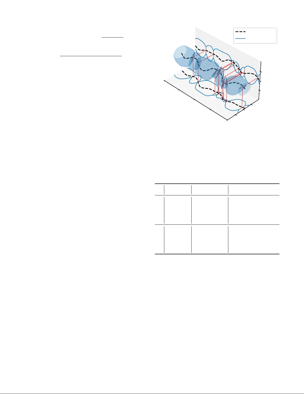
Optimal uncer tainty bounds f or multiv ariate k er nel reg ression under bounded noise: A Gaussian process-based dual function Amon Lahr a , Anna Scampicchio b, ∗ , Johannes K ¨ ohler c, ∗ , Melanie N. Zeilinger a Abstract — Non-conservative uncer tainty bounds are es- sential for making reliab le predictions about latent func- tions from noisy data—and thus, a key enabler for safe learning-based control. In this domain, kernel methods such as Gaussian pr ocess regression are established tech- niques, thanks to their inherent uncertainty quantification mechanism. Still, existing bounds either pose strong as- sumptions on the underlying noise distribution, are con- servative, do not scale well in the multi-output case, or are difficult to integrate into downstream tasks. This paper ad- dresses these limitations by presenting a tight, distribution- free bound for multi-output kernel-based estimates. It is obtained thr ough an unconstrained, duality-based form ula- tion, which shares the same structure of classic Gaussian process confidence bounds and can thus be straightfor- wardl y integrated into downstream optimization pipelines. W e show that the proposed bound g eneralizes many exist- ing results and illustrate its application using an example inspired by quadr otor dynamics learning. Index T erms — Machine learning and control, Estimation, Uncertain systems I . I NT RO D U C T I O N K ERNEL methods hav e recently attracted a lot of at- tention in control due to their accurate estimation per- formance, flexibility and low tuning effort [1]. In particu- lar , estimates from Gaussian process (GP) regression [2], being complemented by rigorous uncertainty bounds, are very promising in view of learning-based control with safety constraints [3]–[5]. Howe ver , standard confidence bounds for Gaussian process regression [6]–[10] cannot handle correlated noise sequences and their probabilistic safety certification does not scale fav orably when the function to be estimated has multiple output dimensions. Deterministic bounds [11]– [16] alleviate this independence assumption, providing robust uncertainty env elopes for bounded noise realizations without asserting a particular noise distribution. Y et, while similarly being restricted to the scalar -output case, e xisting deterministic bounds are either conservati ve [11]–[14], require constrained a Institute f or Dynamical Systems and Control, ETH Zurich, Zurich, Switzerland; { amlahr,mzeilinger } @ethz.ch b Depar tment of Electrical Engineering, Chalmers University of T ech- nology , G ¨ oteborg, Sweden; anna.scampicchio@chalmers.se c Depar tment of Mechanical Engineering, Imperial College London, London, UK; j.kohler@imperial.ac.uk ∗ Both co-authors contributed equally . or non-smooth optimization [15], or are restricted to simple hyper-cube or ellipsoidal uncertainty sets [11]–[16]. In this work, we deri ve a tight, deterministic uncertainty bound in terms of the unconstrained optimizer of a Gaus- sian process-based dual function (Section III). W e extend and generalize the results in [16] to the multiv ariate case as well as to an intersection of ellipsoidal noise bounds, also covering point-wise bounded noise realizations assumed in [11]–[15]. Additionally , we provide a thorough comparison with other existing deterministic bounds, showing that our bound encompasses the ones by [13]–[16] as special cases (Section IV). Finally , we numerically compare the bounds’ conservatism and solve time using an application example inspired by multiv ariate quadrotor dynamics learning subject to direction-dependent wind disturbances (Section V). Notation: The space of (strictly) positive real numbers is denoted by R ≥ 0 ( R > 0 ). W e denote by e i ∈ R N the i -th unit vector in R N , and by 1 N ∈ R N a vector of ones. The weighted Euclidean norm is denoted by ∥ v ∥ M . = √ v ⊤ M v . The concatenation of matrices M i ∈ R n × m is written as [ M i ] N i =1 . = [ M ⊤ 1 , . . . , M ⊤ N ] ⊤ ∈ R N n × m . Like wise, for two ordered index sets I , J ⊆ N with cardinalities | I | = N , | J | = M , particularly for e.g. I N 1 . = 1 : N . = { 1 , . . . , N } , the matrix K f I , J . = [ k ( x i , x j )] i ∈ I ,j ∈ J ∈ R N n f × M n f collects the ev aluations of the (matrix-valued) kernel function k : R n x × R n x → R n f × n f at pairs of input locations x i , x j . I I . P R O B L E M S E T T I N G W e consider the problem of computing uncertainty bounds for the v alue of an unknown multi variate function f tr : R n x → R n f at an arbitrary input location x N +1 ∈ R n x . Information about the latent function is gi ven in terms of a data set of N noisy , partial measurements y = [ y i ] N i =1 ∈ R N , y i = c ⊤ i f tr ( x i ) + w i , ∀ i ∈ I N 1 (1) corrupted by additi ve noise w i . W e assume that the distur- bances w = [ w i ] N i =1 ∈ R N are jointly bounded by a collection of ellipsoidal uncertainty sets, defined as follows. Assumption 1. The noise r ealizations are bounded by w ⊤ P w j w < Γ 2 w,j ∀ j ∈ I n con 1 , (2) with known constants Γ w,j > 0 and positive-semidefinite ma- trices P w j ∈ R N × N . Additionally , the matrix P w . = P n con j =1 P w j is positive definite. Special cases of Assumption 1 include: 1) point-wise bounded noise: For n con = N and P w j = e j e ⊤ j , Eq. (2) reads as w 2 j < Γ 2 w,j , j ∈ I N 1 . 2) energy-bounded noise: For n con = 1 , Eq. (2) reads as w ⊤ P w 1 w < Γ 2 w, 1 , with P w 1 positiv e definite. The special case P w 1 = I N recov ers the setting of energy-bounded noise realizations, i.e., the constraint P N i =1 w 2 i < Γ 2 w, 1 . T o infer uncertainty bounds about the latent function f , we make use of the following standard regularity assumption [6]– [16], cf. [15, Remark 1] for a discussion. Assumption 2. Let f ∈ H k be an element of the Re- pr oducing Kernel Hilbert Space (RKHS) H k , defined by a given positive-semidefinite, matrix-valued kernel function k : R n x × R n x → R n f × R n f . Furthermore , let the norm of f be bounded, i.e., ∥ f ∥ H k < Γ f , for a known constant Γ f > 0 . This general set-up encompasses latent-function estimation using multi variate finite-dimensional features (through positiv e semi-definiteness of k ), independent scalar outputs (through a diagonal structure of k ), or any combination thereof. I I I . M A I N R E S U LT W e formulate the desired uncertainty bound for the vector - valued unknown function in terms of its test-point-dependent, worst-case realization for an arbitrary direction h ∈ R n f . T o this end, we transcribe Assumptions 1 and 2 as well as Eq. (1) into the following optimization problem: f h ( x N +1 ) = sup f ∈H k w ∈ R N h ⊤ f ( x N +1 ) (3a) s . t . c ⊤ i f ( x i ) + w i = y i , i ∈ I N 1 , (3b) w ⊤ P w j w ≤ Γ 2 w,j , j ∈ I n con 1 , (3c) ∥ f ∥ 2 H k ≤ Γ 2 f . (3d) By definition, an optimal solution of Problem (3) determines the optimal worst-case bound for the value of f tr ( x N +1 ) in the direction h , subject to the av ailable information. Conse- quently , the tightest containment interv al along this axis is − f − h ( x N +1 ) ≤ h ⊤ f tr ( x N +1 ) ≤ f h ( x N +1 ) . Our main result derives an optimal solution to Problem (3) using familiar terms from GP regression, using a particular measurement noise cov ariance. T o this end, we denote the multi-output GP posterior mean and cov ariance by f µ σ ( x N +1 ) . = K f N +1 , 1: N C ˆ K − 1 σ y , (4) Σ f σ ( x N +1 ) . = K f N +1 ,N +1 − K f N +1 , 1: N C ˆ K − 1 σ C ⊤ K f 1: N ,N +1 , respectiv ely . The matrix ˆ K σ . = C ⊤ K f 1: N , 1: N C + K w σ denotes the Gram matrix, where the matrix K f 1: N , 1: N of kernel ev alua- tions on the training inputs is projected using the measurement matrix C ⊤ . = blkdiag  c ⊤ 1 , . . . , c ⊤ N  ∈ R N × n f N , defined according to the linear measurement model (1). While K w σ commonly denotes the cov ariance of (possibly correlated) Gaussian measurement noise, here we define K w σ . = ( P w σ ) − 1 . =   n con X j =1 σ − 2 j P w j   − 1 (5) based on the ellipsoidal noise bounds (2) and a fr ee vector of noise parameters σ = [ σ j ] n con j =1 ∈ R con > 0 . For special case 1) of Assumption 1, note that K w σ = diag( σ 2 1 , . . . , σ 2 N ) corresponds to assuming independent, heteroscedastic noise; for special case 2), i.e., K w σ = σ 2 1 ( P w 1 ) − 1 , the scalar parameter σ 1 can be interpreted as the output scale for an unknown noise- generating process [16, Sec. 3.1]. W e are now ready to state our main result. Theorem 1. Let Assumptions 1 and 2 hold and define f σ h ( x N +1 ) . = h ⊤ f µ σ ( x N +1 ) + β σ q h ⊤ Σ σ ( x N +1 ) h, (6) with β σ . = v u u t Γ 2 f + n con X j =1 Γ 2 w,j σ 2 j − ∥ y ∥ 2 ˆ K − 1 σ . (7) Then, for any h ∈ R n f and any x N +1 ∈ R n x , i) h ⊤ f tr ( x N +1 ) ≤ f σ h ( x N +1 ) for all σ ∈ R n con > 0 ; ii) the optimal uncertainty bound (3) is given by f h ( x N +1 ) = inf σ ∈ R n con > 0 f σ h ( x N +1 ); (8) iii) f σ h ( x N +1 ) is in vex: σ ⋆ ∈ R n con > 0 is a global minimizer of Pr oblem (8) if and only if ∂ ∂ σ f σ h ( x N +1 )    σ = σ ⋆ = 0 . The proof of Theorem 1, reported in Section B, mainly relies on strong duality of a finite-dimensional representation of Problem (3). In particular , the function f σ h ( x N +1 ) , which corresponds to β σ -confidence bounds of the multivariate GP posterior in the direction h , is shown to be a reparametriza- tion of the dual function of Problem (3), establishing state- ments i) and ii) by weak and strong duality , respectively . For the reparametrization, the optimal dual variable λ 0 for the complexity constraint (3d) is determined in closed form and the noise parameters [ σ 2 j ] n con j =1 . = [ λ 0 λ j ] n con j =1 are in versely proportional to the dual v ariables [ λ j ] n con j =1 for each respectiv e constraint (3c). The scaling factor β σ can be interpreted as the total RKHS norm in a data-generating RKHS, subtracted by the RKHS norm of the corresponding minimum-norm interpolant, cf. [16, Eq. (6)]. Statement i) of Theorem 1 establishes a v alid, yet potentially conservati ve uncertainty bound for all noise parameters σ ∈ R n con > 0 . Noting that this upper bound is giv en by the projection of the multi v ariate GP posterior in the direction h for a fixed vector of noise parameters, we can deriv e the following ellipsoidal uncertainty bound. Corollary 1. Let Assumptions 1 and 2 hold. Then, ∀ σ ∈ R n con > 0 ∥ f tr ( x N +1 ) − f µ σ ( x N +1 ) ∥ Σ f ( x N +1 ) − 1 ≤ β σ . (9) Pr oof. Using h = Σ( x N +1 ) − 1 ( f tr ( x N +1 ) − f µ σ ( x N +1 )) , the assertion is obtained by rearranging Theorem 1, point i). An essential adv antage of the duality-based, unconstrained bound formulation in Theorem 1, i) and Corollary 1 is their straightforward integration into downstream optimization tasks: the dual (noise) parameters σ can be simultaneously optimized alongside the primary objective, tightening the uncertainty bound as necessary for the downstream task while guaranteeing safe predictions at each iteration. In ve xity in statement iii) is deri ved from the unique mapping between the original dual v ariables and the noise parameters σ , and the conca vity of the original dual function. It guarantees that any local minimizer in the open domain R n con > 0 is globally optimal, rendering the bound attractiv e for scalable gradient- based optimization. Note, howe ver , that the in ve xity property does not guarantee attainment of the optimizer in the open domain R n con > 0 : indeed, the optimal bound in Eq. (8) might be attained only in the limit for some σ j → 0 or σ j → ∞ . Illustrativ e example: Fig. 1 illustrates Theorem 1 for a simple example, where the proposed uncertainty bound is computed for a random unknown function f tr ∈ H k with the squared- exponential kernel k ( x, x ′ ) = exp( −∥ x − x ′ ∥ 2 2 ) , a known RKHS-norm bound Γ 2 f = 1 and N = 2 training points corrupted by point-wise bounded noise realizations | w j | ≤ 0 . 2 [equiv alent to special case 1) of Assumption 1 with Γ w,j = 0 . 2 ]. The optimal value of the dual function coincides with the optimal uncertainty bound at each respective test point due to strong duality; additionally , weak duality ensures that it also provides a conservati ve bound for the whole domain. The incurred conservatism depends on the value of the noise parameters σ : for [ σ ] n con j =1 → ∞ , the uncertainty bound (6) con ver ges to the prior bound, f σ h ( x ) → Γ f p h ⊤ k ( x, x ) h ; if any σ j → 0 , it may grow unbounded; cf. [16, Sec. 3.3] for a detailed discussion. − 0 . 5 0 . 0 0 . 5 1 . 0 Uncertainty bounds true function data lower bound upper bound 10 − 2 10 0 10 2 σ ∗ 1 0 . 0 0 . 5 1 . 0 1 . 5 2 . 0 2 . 5 3 . 0 3 . 5 x N + 1 10 − 2 10 0 10 2 σ ∗ 2 Fig. 1. Illustrativ e example of proposed uncer tainty bound. The top plot shows the optimal uncer tainty bounds (solid), as well as the corresponding dual functions (shaded), e valuated for the optimal dual (noise) parameters σ ⋆ at the test point x N +1 = 1 . 5 (dotted red). The bottom two plots show the corresponding optimal value of the dual (noise) parameters σ ⋆ for all test points. I V . D I S C U S S I O N In this section, we compare the proposed bound with av ailable kernel regression bounds. Since all a vailable results are presented in the scalar -output case, we restrict the following discussion to n f = 1 . 1) Optimal deter ministic bounds (optimization-based) : The proposed bound generalizes the optimal deterministic bounds dev eloped by [15] and [16] for point-wise bounded and energy-bounded noise realizations, which are both recov ered as special cases 1) and 2) of Assumption 1, respectiv ely . For point-wise bounded noise, assuming a uniform noise bound | w i | ≤ ¯ Γ w and a positive-definite kernel function k , [15] also provides a duality-based formulation of their bound, f h ( x N +1 ) = inf ν ∈ R N , λ> 0 y ⊤ ν + ¯ Γ w ∥ ν ∥ 1 + λ Γ 2 f (10) + 1 4 λ  K f N +1 ,N +1 + ∥ C ν ∥ 2 K f 1: N, 1: N − 2 K f N +1 , 1: N C ν  . Compared with the proposed dual objecti ve in Theorem 1, which is in ve x and smooth, the dual objectiv e (10) is con ve x and non-smooth. T o address non-smoothness, [15, Alg. 1] pro- poses an alternating-optimization procedure, iterating closed- form optimization of the scalar multiplier λ and 1-norm- constrained quadratic minimization of ν ∈ R N . While this algorithm is found to be ef fectiv e for iterating towards the optimal uncertainty bound (see Section V), it remains difficult to integrate into do wnstream (optimization) tasks as it still in volv es inequality constraints. In contrast, the proposed dual objectiv e (6) is straightforwardly integrated into optimization pipelines, optimizing σ as part of the do wnstream objective. For energy-bounded noise, Theorem 1 encompasses [16, Theorem 1], which equiv alently expresses the optimal uncer- tainty bound in terms of unconstrained optimization of the (scalar) noise parameter σ . This paper extends these results by additionally showing inv exity of the dual function (6). Moreov er , the duality-based viewpoint of the upper bound simplifies the proof, cf. [16, Appendix C], while explaining the potential conservatism of existing suboptimal, closed-form bounds as discussed in the follo wing. 2) Suboptimal deter ministic bounds (closed-form) : A vailable closed-form, suboptimal bounds in the bounded-noise setting can be classified into two types. First, utilizing the Cauchy-Schwarz inequality for an inner product defined by the posterior kernel k ( · , · ) − K f · , 1: N ˆ K − 1 σ K f 1: N , · , cf. [6, Lemma 7.2], the works [13, Lemma 2] and [14, Lemma 2] obtain a bound of the form | f tr ( x N +1 ) − f µ σ ( x N +1 ) | ≤ β σ p Σ σ ( x N +1 ) (11) for a fixed value of σ = ¯ σ 1 N and a uniform noise bound | w i | ≤ ¯ Γ w for all i ∈ I N 1 . In this case, the scaling factor β σ in Eq. (4) simplifies to β 2 σ = Γ 2 f + N ¯ Γ 2 w ¯ σ − 2 − ∥ y ∥ 2 ˆ K − 1 σ , with ¯ σ 2 = ¯ Γ 2 w and ¯ σ 2 = N ¯ Γ 2 w for [13] and [14], respecti vely . These bounds are recovered by Corollary 1 for point-wise bounded noise [special case 1) of Assumption 1], showing that their conservatism can be attributed to the fact that they correspond to an ev aluation of the dual function (6) for a fixed set of dual (noise) parameters. Second, in [11], [12], [15], suboptimal, closed-form uncer- tainty bounds are obtained by separating the prediction error in an interpolation- and a noise-error term. For example, the bound formulated in [12, Theorem 2] reads as | f tr ( x N +1 ) − f µ σ ( x N +1 ) | ≤ β f max p Σ σ ( x N +1 ) + ¯ Γ w ∥ ˆ K − 1 σ K f 1: N ,N +1 ∥ 1 , (12) where β f max . = q Γ 2 f − min | w i |≤ ¯ Γ w ∥ y − w ∥ 2 ˆ K − 1 σ . This formu- lation generalizes the ones in [11, Theorem 1], [15, Proposi- tion 3] in that it allo ws for an arbitrary noise parameter ¯ σ > 0 , with σ = ¯ σ 1 N . In contrast, the preceding works are restricted to ¯ σ = 0 in the interpolation term (which comes with the additional limitation to positi ve-definite kernels and unique training input locations), and bound the difference to the actual mean prediction f µ σ separately using the triangle inequality . Despite the additional conservatism incurred by the separation of errors, one advantage of these bounds is that the value of the uncertainty bound stays bounded as ¯ σ → 0 . Still, the ev aluation of the scaling factor β f max requires solving a quadratic program comparable in complexity to (10) whenev er the data set is modified. 3) Finite-dimensional h ypothesis spaces : Since our theoreti- cal analysis applies to general positi ve-semidefinite kernels (cf. Assumption 2), it applies to the classical special case of linear regression with a finite-dimensional hypothesis spaces, i.e., k ( x, x ′ ) = Φ( x )Φ( x ′ ) ⊤ for some features Φ : R n x → R n f × r . In terms of application to control, this can, e.g., be used for estimating (non-falsified) nonlinear system dynamics from noisy measurements, where the noise at each time step is bounded by a quadratic constraint (2), cf. [5, Sec. 5]. In the special case of a single quadratic noise constraint, our result recov ers classical analytical regression bounds under energy- bounded noise [17]; see also [16, Sec. 4.1] for a discussion. 4) Probabilistic bounds : The proposed bound shares the same structure with many probabilistic results, where (11) holds with some user-defined confidence 1 − δ , and measure- ment noise realizations are assumed to be conditionally zer o- mean R -sub-Gaussian [18]. This different setting is reflected in the expressions for the scaling factor β σ , which commonly feature both the variance proxy R and the parameter δ en- forcing the desired confidence lev el, cf., e.g., [9, Eq. (7)]. The main limitation of these bounds is their strong assumption on the measurement noise, prev enting them from rigorously handling biased, correlated and adversarial disturbances— all scenarios encompassed by the proposed distribution-free bounds. Moreov er , they can handle only increasing training data-set sizes: as such, differently from the proposed ap- proach, they cannot be applied to subset-of-data strategies to improv e scalability . Further discussions can be found in [15, Section VI, Example 1] and [16, Section 4.3]. V . A P P L I C A T I O N E X A M P L E In the following, we compare the proposed bound with existing bounds using an application example inspired by dynamics learning in control 1 . Here, the task is to estimate the residual acceleration f tr ( x ) = ( a x ( θ ) , a z ( θ )) ∈ R 2 of 1 The full source code and implementation details are available at https: //gitlab.ethz.ch/ics/bounded- rkhs- bounds- duality . 0 π / 2 π 3 π / 2 2 π θ − 10 0 10 a x ( θ ) − 10 0 10 a y ( θ ) true function Dual-GD (e) Fig. 2. Proposed multivariate uncertainty bound f or quadrotor example with n data = 10 training points. The latent function (dashed blac k) is tightly bounded by the optimal uncer tainty bounds ev aluated for both output dimensions (Theorem 1); the multivariate ellipsoidal tube is generated using σ -v alues corresponding to the optimal upper bound in x -direction (Corollar y 1). The (projected) data points and (projected) uncer tainty bounds are shown in red and gray , respectively . T ABLE I E X P E R I M E N TAL R E S U LT S F O R T H E Q U A D R OT O R E X A M P L E Method Suboptimality T ime [s] min. avg. max. min. avg. max. n data = 100 CVX-full (e) 0.00 0.00 0.00 0.55 0.66 3.16 CVX-full (p) 0.01 0.22 0.70 0.13 0.19 0.27 [15] (p) 0.01 0.22 0.70 0.00 0.02 0.07 [12] (p) 0.31 0.70 2.09 0.01 0.01 0.03 Dual-GD (e) 0.00 0.00 0.03 0.40 1.46 1.84 Dual-GD (p) 0.01 0.23 0.70 0.21 0.76 1.55 n data = 1000 CVX-full (e) 0.00 0.00 0.00 289.66 302.84 326.85 CVX-full (p) 0.00 0.19 0.62 32.88 34.19 49.30 [15] (p) 0.00 0.19 0.62 0.92 2.68 26.83 [12] (p) 0.46 0.71 1.30 0.04 0.05 0.11 Dual-GD (e) 0.03 0.15 0.39 3.45 5.10 16.70 Dual-GD (p) 0.18 0.37 0.79 0.76 1.07 2.27 a two-dimensional quadrotor in body frame as a function of its tilt angle θ ∈ [0 , 2 π ] ( n x = 1) , based on noisy measurements of its acceleration a x , a z in both components ( n f = 2) . The latent function f tr is randomly generated using a periodic kernel, enforcing the RKHS-norm bound Γ 2 f = 1 . The n data ∈ { 100 , 1000 } measurements are corrupted by an unknown wind force, which is assumed to be contained within a 2D ellipsoid with differently scaled semi-axes in the global coordinate frame, resulting in tilt-angle-dependent, ellipsoidal noise bounds P w j ( θ ) , j ∈ I n data 1 . The components of each measurement are extracted by defining c ⊤ i,x =  1 0  and c ⊤ i,z =  0 1  , resulting in a total of N = 2 n data data points. Fig. 2 depicts this setup for n data = 10 measurements. The following methods are compared in T able I: “CVX- full” solves the finite-dimensional version of Problem (3), see Section A, using CVXPY [19]; “[15]” implements the iterative algorithm discussed in Section IV -.1 in CVXPY [19]; “[12]” computes the closed-form bound in Eq. (12) with ¯ σ = ¯ Γ w set to the uniform noise error bound 2 ; “Dual-GD” optimizes Problem (8) with GPyTorch [20] using the accelerated gradi- ent descent method Adam with a fixed learning rate of 0.1. T o compare the conservatism resulting from the ellipsoidal “(e)” or the corresponding smallest uniform point-wise “(p)” noise bound ¯ Γ w imposed by [12], [15], we additionally implement a variant using the latter noise assumption. This v ariant results in a reduced number of N = n data data points since only measurements for the respecti v e coordinate are utilized. T able I shows the suboptimality and computation time (minimum, mean, and maximum), indicating the dif ference to the optimal uncertainty bound “CVX-full (e)”, normalized by the differ - ence of the prior uncertainty bound. The following stopping times are selected: for “CVX-full”, until con ver gence; for [15, Alg. 1], until 10 − 2 suboptimality with respect to “CVX-full (p)”; for “Dual-GD”, after 100 gradient steps. The results indicate that [15, Alg. 1] con ver ges reliably and quickly to the optimal uncertainty bound assuming pointwise- bounded noise realizations, explaining the remaining dif fer- ence to the optimal solution utilizing the ellipsoidal noise bound. The closed-form bound in [12, Theorem 2] naturally achiev es the lo west computational time; ho wev er , it also sho ws the highest conservatism. For Dual-GD, reliable con ver gence to the optimal solution is observed for n data = 100 . For n data = 1000 , con ver gence is challenged by the high density of training points, which leads to more than 95% of the optimal values σ ⋆ j → ∞ at the boundary of the domain for both noise assumptions. Ne vertheless, it ef fecti vely reduces the size of the uncertainty bound in the limited number of iterations, leading to competitiv e uncertainty estimates. V I . C O N C L U S I O N S W e have deriv ed a tight, deterministic uncertainty bound for k ernel-based worst-case uncertainty quantification. The duality-based formulation extends the applicability of kernel- based uncertainty bounds to the multiv ariate case and more complex noise descriptions, while unifying a range of existing results in the literature. Enabled by the unconstrained problem formulation, the numerical results highlight the effecti veness of the bound in reducing the size of the uncertainty en ve- lope, motiv ating its application to downstream tasks such as Bayesian optimization or safe learning-based control. R E F E R E N C E S [1] B. Sch ¨ olkopf and A. J. Smola, Learning with Kernels: Support V ector Machines, Re gularization, Optimization, and Beyond , ser . Adaptive Computation and Machine Learning. Cambridge, Mass: MIT Press, 2002. [2] C. E. Rasmussen and C. K. I. Williams, Gaussian Pr ocesses for Machine Learning , ser . Adaptive Computation and Machine Learning. Cambridge, Massachusetts: MIT Press, 2006. [3] A. Scampicchio, E. Arcari, A. Lahr, and M. N. Zeilinger, “Gaussian processes for dynamics learning in model predictive control, ” Annual Reviews in Contr ol , vol. 60, 2025. [4] K. P . W abersich, A. J. T aylor, J. J. Choi, K. Sreenath, C. J. T omlin, A. D. Ames, and M. N. Zeilinger , “Data-Dri ven Safety Filters: Hamilton- Jacobi Reachability, Control Barrier Functions, and Predictiv e Methods for Uncertain Systems, ” IEEE Contr ol Systems Magazine , vol. 43, no. 5, 2023. 2 Different tested choices ¯ σ ∈ { 10 − 3 , ¯ Γ w , 10 3 } lead to similar results, with ¯ σ = ¯ Γ w achieving the lowest suboptimality . [5] T . Martin, T . B. Sch ¨ on, and F . Allg ¨ ower , “Guarantees for data-driv en control of nonlinear systems using semidefinite programming: A surve y , ” Annual Reviews in Control , vol. 56, 2023. [6] N. Sriniv as, A. Krause, S. M. Kakade, and M. W . Seeger , “Information- Theoretic Regret Bounds for Gaussian Process Optimization in the Bandit Setting, ” IEEE T ransactions on Information Theory , vol. 58, no. 5, 2012. [7] Y . Abbasi-Y adkori, “Online learning for linearly parametrized control problems, ” Ph.D. dissertation, University of Alberta, Edmonton, Alberta, 2013. [8] S. R. Chowdhury and A. Gopalan, “On Kernelized Multi-armed Ban- dits, ” in Proceedings of the 34th International Conference on Machine Learning . PMLR, 2017. [9] C. Fiedler , J. Menn, L. Kreisk ¨ other , and S. Trimpe, “On safety in safe bayesian optimization, ” Tr ansactions on Machine Learning Researc h , 2024. [10] O. Molodchyk, J. T eutsch, and T . Faulwasser , “T o wards safe Bayesian optimization with W iener kernel regression, ” in 2025 European Control Confer ence (ECC) , 2025. [11] E. T . Maddalena, P . Scharnhorst, and C. N. Jones, “Deterministic error bounds for kernel-based learning techniques under bounded noise, ” Automatica , vol. 134, 2021. [12] R. Reed, L. Laurenti, and M. Lahijanian, “Error Bounds for Gaussian Process Regression Under Bounded Support Noise with Applications to Safety Certification, ” Proceedings of the AAAI Conference on Artificial Intelligence , vol. 39, no. 19, 2025. [13] K. Hashimoto, A. Saoud, M. Kishida, T . Ushio, and D. V . Dimarogonas, “Learning-based symbolic abstractions for nonlinear control systems, ” Automatica , vol. 146, 2022. [14] Z. Y ang, X. Dai, W . Y ang, B. Ilgen, A. Anzel, and G. Hattab, “Kernel- based Learning for Safe Control of Discrete-Time Unknown Systems under Incomplete Observations, ” in 2024 43rd Chinese Contr ol Confer- ence (CCC) , 2024. [15] P . Scharnhorst, E. T . Maddalena, Y . Jiang, and C. N. Jones, “Robust Uncertainty Bounds in Reproducing Kernel Hilbert Spaces: A Conv ex Optimization Approach, ” IEEE T ransactions on Automatic Contr ol , vol. 68, no. 5, 2023. [16] A. Lahr, J. K ¨ ohler , A. Scampicchio, and M. N. Zeilinger, “Optimal kernel regression bounds under energy-bounded noise, ” 2025, to be published in Advances in Neural Information Processing Systems, doi:10.48550/arXiv .2505.22235. [17] E. Fogel, “System identification via membership set constraints with energy constrained noise, ” IEEE T ransactions on Automatic Control , vol. 24, no. 5, 1979. [18] C. Fiedler , C. W . Scherer, and S. Trimpe, “Practical and Rigorous Uncertainty Bounds for Gaussian Process Regression, ” Pr oceedings of the AAAI Conference on Artificial Intelligence , vol. 35, no. 8, 2021. [19] S. Diamond and S. Boyd, “CVXPY: A Python-embedded modeling lan- guage for con vex optimization, ” Journal of Machine Learning Research , vol. 17, no. 83, 2016. [20] J. Gardner , G. Pleiss, K. Q. W einberger , D. Bindel, and A. G. Wilson, “GPyT orch: Blackbox Matrix-Matrix Gaussian Process Inference with GPU Acceleration, ” in Advances in Neural Information Processing Systems , vol. 31. Curran Associates, Inc., 2018. [21] S. P . Boyd and L. V andenberghe, Conve x Optimization . Cambridge, UK ; New Y ork: Cambridge University Press, 2004. A P P E N D I X A. Auxiliary results Lemma 1. The optimal solution to (3) coincides with the solution to the following finite-dimensional con ve x pr ogram f h ( x N +1 ) = sup θ ∈ R r h ⊤ Φ N +1 θ (13a) s . t . ∥ θ ∥ 2 2 ≤ Γ 2 f , (13b) ∥ y − C ⊤ Φ 1: N θ ∥ 2 P w j ≤ Γ 2 w,j , (13c) for j ∈ I n con 1 . The feature matrix Φ 1: N +1 . = [Φ i ] N +1 i =1 ∈ R n f ( N +1) × r , with full column rank r ≤ n f ( N + 1) , composed of feature evaluations Φ i ∈ R n f × r at input locations x i , is given by the Gram matrix factorization K f 1: N +1 , 1: N +1 . = [ k ( x i , x j )] N +1 i,j =1 = Φ 1: N +1 Φ ⊤ 1: N +1 ∈ R n f ( N +1) × n f ( N +1) . Pr oof. The result is deri ved using adaptation of the representer theorem, following the steps in [16, Appendix A]. Lemma 2. Str ong duality holds for Problem (13) . Pr oof. Let f tr , int = arg min f ∈H k ∥ f ∥ 2 H k (14a) s . t . f ( x i ) = f tr ( x i ) , i ∈ I N +1 1 (14b) be the minimum-norm interpolant of f tr at the training- and test-inputs. By the representer theorem [1, Ch. 4.2], f tr , int ( x N +1 ) = Φ N +1 θ tr . Hence, ∥ θ tr ∥ 2 = ∥ f tr , int ∥ H k ≤ ∥ f tr ∥ H k < Γ f , where the final inequality follo ws from Assumption 2, establishing θ tr as a strictly feasible point of the conv ex program (13). Thus, Slater’ s condition [21, Chap. 5.2.3] is satisfied, yielding the claim. B. Proof of Theorem 1 1) Proof of statements i) and ii) : The optimal solution to the infinite-dimensional problem (3) coincides with the op- timal solution of the finite-dimensional, con ve x program (13) (cf. Lemma 1). The Lagrangian of (13) is L ( θ , λ 0: n con ) = h ⊤ Φ N +1 θ − λ 0  ∥ θ ∥ 2 2 − Γ 2 f  − n con X j =1 λ j  ∥ y − C ⊤ Φ 1: N θ ∥ 2 P w j − Γ 2 w,j  , (15) and d ( λ 0: n con ) = sup θ L ( θ , λ 0: n con ) is its concav e dual function. Due to strong duality (cf. Lemma 2), the optimal solution to (13) is equal to the dual solution f h ( x N +1 ) = inf λ 0 ,...,λ n con ≥ 0 d ( λ 0: n con ) . (16) By defining the “partially-minimized” dual function d 0 ( λ 1: n con ) = inf λ 0 ≥ 0 sup θ L ( θ , λ 0: n con ) , we can write Problem (16) as f h ( x N +1 ) = inf λ 1 ,...,λ n con ≥ 0 d 0 ( λ 1: n con ) . Due to continuity of the dual function with respect to the dual variables λ , we can assume λ j > 0 , j ∈ I n con 0 , without loss of generality: by the definition of the infimum, it holds that inf λ 0: n con ≥ 0 d ( λ 0: n con ) = inf λ 0: n con > 0 d ( λ 0: n con ) . Hence, we can reparametrize the original Lagragian (15) as L σ ( θ , λ 0 , σ 1: n con ) = h ⊤ Φ N +1 θ − λ 0  ∥ θ ∥ 2 2 − Γ 2 f  − λ 0  ∥ y − C ⊤ Φ 1: N θ ∥ 2 P w σ − Γ 2 w,j  , (17) with L σ ( θ , λ 0 , σ 1: n con ) = L ( θ , λ 0: n con ) for the dual (noise) parameter [ σ 2 j ] n con j =1 = [ λ 0 λ j ] n con j =1 . W e analogously reparametrize d σ 0 ( σ 1: n con ) = inf λ 0 > 0 sup θ L σ ( θ , λ 0 , σ 1: n con ) and re- cov er the original optimal solution (16) as f h ( x N +1 ) = inf σ 1 ,...,σ n con ∈ (0 , ∞ ) d σ 0 ( σ 1: n con ) . (18) Finally , we deriv e d σ 0 ( σ 1: n con ) in closed form by noting that it is the dual solution for the primal problem f σ h ( x N +1 ) = sup θ ∈ R r h ⊤ Φ N +1 θ (19a) s . t . ∥ θ ∥ 2 2 + ∥ y − C ⊤ Φ 1: N θ ∥ 2 P w σ ≤ Γ 2 f + n con X j =1 Γ 2 w,j σ 2 j . (19b) The analytical solution to this con ve x program with linear cost and a single quadratic constraint is (see Section C) f σ h ( x N +1 ) = h ⊤ f µ σ ( x N +1 ) + β σ q h ⊤ Σ σ ( x N +1 ) h. (20) For Problem (19), strong duality is established using the same strictly feasible point as in Lemma 2, since ev ery (strictly) feasible solution to (13) is a (strictly) feasible solution to (19). W ith f σ h ( x N +1 ) = d σ 0 ( σ 1: n con ) , inserting Eq. (20) in Eq. (18) giv es statement i): h ⊤ f tr ( x N +1 ) ≤ f h ( x N +1 ) ≤ f σ h ( x N +1 ) ; statement ii) follows directly from Eq. (18). 2) Proof of statement iii) : Let ∂ ∂ σ f σ h ( x N +1 ) = 0 for some σ ⋆ ∈ R n con + . Since f σ h ( x N +1 ) = d σ 0 ( σ ⋆ 1: n con ) , it holds that ∂ ∂ σ d σ 0 ( σ ⋆ 1: n con ) = 0 . Using the reparametrization ( σ ⋆ j ) 2 = λ 0 λ ⋆ j , j ∈ I n con 1 , we obtain that ∂ ∂ λ 1: n con d 0 ( λ ⋆ 1: n con ) = 0 . As d σ 0 ( x N +1 ) is the restriction of the conv ex dual func- tion d ( λ 0: n con ) through partial maximization of its λ 0 - component ov er the con v ex set λ 0 ∈ (0 , ∞ ) , it is con vex [21, Chap. 3.2.5]. Therefore, λ ⋆ 1: n con is the global minimizer of problem (16), which implies the assertion that f σ h ( x N +1 ) = f h ( x N +1 ) with σ = σ ⋆ is globally optimal. C . Proof of Eq. (20) The claim follows by re-writing (19) through a suitable reparametrization. First, consider (19) and let h ⊤ Φ N +1 . = q ⊤ , C ⊤ Φ 1: N . = A ⊤ and Γ 2 f + P n con j =1 σ − 2 j Γ 2 w,j . = Γ 2 ; additionally , define S . = I + AP w σ A ⊤ with matrix square-root S = S 1 / 2 S 1 / 2 . Finally , let θ µ σ . = A  A ⊤ A + ( P w σ ) − 1  − 1 y = S − 1 AP w σ y be the vector yielding the finite-dimensional parametrization of the GP posterior mean f µ σ ( x N +1 ) = Φ N +1 θ µ σ . This allows us to rewrite (19b) as ∥ θ − θ µ σ ∥ 2 S + ∥ y ∥ 2 ˆ K − 1 σ ≤ Γ 2 , (21) where we have used that P w σ − P w σ A ⊤ S − 1 AP w σ =  A ⊤ A + ( P w σ ) − 1  − 1 = ˆ K − 1 σ entering (4). Using Eq. (21) and a change of coordinates ξ . = S 1 / 2 ( θ − θ µ σ ) , we can re write problem (19) as a linear problem with norm-ball constraint: f σ h ( x N +1 ) = sup ξ ∈ R r q ⊤ θ µ σ + q ⊤ S − 1 / 2 ξ s . t . ∥ ξ ∥ 2 2 ≤ Γ 2 − ∥ y ∥ 2 ˆ K − 1 σ . The unique optimal solution is ξ ⋆ = q Γ 2 − ∥ y ∥ 2 ˆ K − 1 σ S − 1 / 2 q ∥ q ∥ S − 1 , defining the v alue of the worst-case latent function at the test point: f ⋆ ( x N +1 ) = Φ N +1 θ ⋆ = Φ N +1 ( θ µ σ + S − 1 / 2 ξ ⋆ ) . W ith ∥ q ∥ 2 S − 1 = q ⊤  I − A  A ⊤ A + ( P w σ ) − 1  − 1 A ⊤  q = h ⊤ Φ N +1  I − Φ ⊤ 1: N C ˆ K − 1 σ C ⊤ Φ 1: N  Φ ⊤ N +1 h = h ⊤ Σ σ ( x N +1 ) h, this leads to the sought optimal value f σ h ( x N +1 ) = q ⊤ θ µ σ + q Γ 2 − ∥ y ∥ 2 ˆ K − 1 σ ∥ q ∥ S − 1 = h ⊤ f µ σ + β σ q h ⊤ Σ f σ ( x N +1 ) h.