Linearized Bregman Iterations for Sparse Spiking Neural Networks

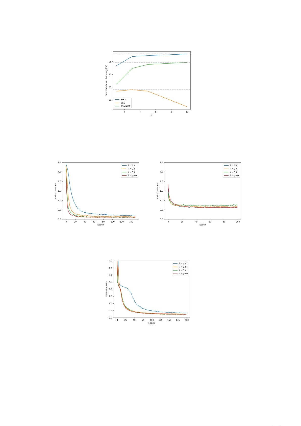
Linearized Br egman Iterations f or Sparse Spiking Neural Networks Daniel Windhager Silicon Austria Labs Linz, Austria daniel.windhager@silicon-austria.com Bernhard A. Moser ∗ Software Competence Center Hagenber g Hagenberg, Austria bernhard.moser@scch.at Michael Lunglmayr Institute of Signal Processing Johannes Kepler Uni v ersity Linz, Austria michael.lunglmayr@jku.at Abstract Spiking Neural Networks (SNNs) offer an energy ef ficient alternativ e to con v en- tional Artificial Neural Networks (ANNs) but typically still require a large number of parameters. This work introduces Linearized Br e gman Iterations (LBI) as an optimizer for training SNNs, enforcing sparsity through iterative minimization of the Bregman distance and proximal soft thresholding updates. T o improv e con ver gence and generalization, we employ the AdaBr eg optimizer , a momentum and bias corrected Bregman variant of Adam. Experiments on three established neuromorphic benchmarks, i.e. the Spiking Heidelberg Digits (SHD), the Spik- ing Speech Commands (SSC), and the Permuted Sequential MNIST (PSMNIST) datasets, sho w that LBI based optimization reduces the number of acti ve parameters by about 50% while maintaining accuracy comparable to models trained with the Adam optimizer , demonstrating the potential of con ve x sparsity inducing methods for efficient neuromorphic learning. 1 Introduction Sparsity in neural networks is an important and ongoing research field Hoefler et al. [ 2021 ]. In most neural network architectures sparsity refers to the weight matrices of the model being sparsely populated. This has the effect of sparsifying connections of the network (i.e. a connection with weight 0 is disconnected). For classical GPU implementations, howe v er , ha ving sparse weights can sometimes actually lead to increased computational ov erhead due to memory organization problems and unbalanced w orkloads Zaharia et al. [ 2020 ]. In contrast, for edge AI implementations where network structures are directly mapped to hardw are, e.g. as in W indhager et al. [ 2025 ], the benefits are considerably higher as the sparsity of weights can be utilized and exploited more easily . T raining machine learning to produce sparse weight matrices is in essence a sparse optimization problem. In practice, sparsity is often achieved through heuristic approaches such as pruning Hoefler et al. [ 2021 ], ev en though there exist mathematically founded algorithms that can prov ably con ver ge to sparse optimal solutions. A number of these algorithms is based on so-called linearized Bregman iterations, which hav e also been proposed for sparse estimation Osher et al. [ 2005 ], Y in et al. [ 2008 ] using concepts similar to Douglas–Rachford splitting Combettes and Eckstein [ 1992 ]. Their efficienc y ∗ double affiliation with Institute of Signal Processing, Johannes K epler Uni versity Linz The Second Austrian Symposium on AI and V ision (AIRO V25). and stability for sparse estimation have been demonstrated repeatedly Hu and Chklo vskii [ 2014 ], Gebhard et al. [ 2018 ], and more recent work has shown their suitability for training sparse deep neural networks, in many cases outperforming heuristic solutions Bungert et al. [ 2022 ]. In this work, we in vestig ate ho w linearized-Bregman-based sparse learning performs for spiking neural networks. Specifically , we ev aluate both feedforward and recurrent SNN architectures on established neuromorphic benchmarks and analyze how the re gularization parameter λ influences sparsity and model accuracy . 2 Linearized Bregman Iterations Sparse optimization problems often include a regularization term J ( θ ) based on the ℓ 1 -norm to promote sparsity . Howe ver , the non-smoothness of the ℓ 1 -norm causes standard gradient-based optimization to fail in regions where the gradient is undefined. A key property that enables a well- behav ed optimization frame work in such cases is the con ve xity of the re gularization function J . For con ve x b ut possibly non-smooth functions, the concept of a gradient is replaced by a sub-differ ential , which generalizes differentiation to non-smooth settings. Sub-dif ferentials, ho wev er , can not directly be used in steepest-decent like algorithms as they require a defined gradient at each step. T o handle such cases, Bregman iterations iterativ ely minimize the Bre gman distance Bre gman [ 1967 ] D J ( x, y ) = J ( x ) − J ( y ) − ⟨∇ J ( y ) , x − y ⟩ , rather than minimizing the composite cost function directly . In this formulation, ∇ J ( y ) represents an element of the sub-differ ential of J at point y , denoted ∂ J ( y ) . For con vex J , the sub-differentia l ∂ J ( y ) is a non-empty , con ve x set that captures all possible slopes of local supporting hyperplanes to J at y . For example, when J ( x ) = | x | , the sub-differential at x = 0 is the interval [ − 1 , 1] . This interpretation allows the Bregman distance to generalize classical gradient-based methods to con ve x but non-diff erentiable regularizers, enabling optimization for the ℓ 1 -norm and similar sparsity-promoting terms. Because the resulting subproblems rarely admit closed-form solutions for sparse re gularizers Y in et al. [ 2008 ], the Linearized Br e gman Iteration (LBI) method provides an efficient linearized approximation. LBI introduces auxiliary “shado w” v ariables v corresponding to the model parameters θ . At iteration t , the updates can be expressed as v ( t +1) = v ( t ) + µ ∇ L ( θ ( t ) , B ) , θ ( t +1) = prox J ( v ( t +1) ) , where µ denotes the step size and prox J represents the proximal operator associated with the conv ex regularization term J . For the commonly used sparse re gularizer J ( θ ) = λ ∥ θ ∥ 1 , the proximal operator corresponds to the elementwise soft-thr esholding function, prox λ ∥ θ ∥ 1 ( θ ) = h prox λ ∥ θ ∥ 1 ( θ i ) i i (1) prox λ ∥ θ ∥ 1 ( θ i ) = sign ( θ i ) max(0 , | θ i | − λ ) , (2) which suppresses small weight values and dri v es many parameters exactly to zero, thereby yielding sparse network representations. This mechanism makes LBI particularly well suited for training models such as Spiking Neural Networks, where conv ex sparse regularization aligns well with the need for energy-ef ficient, low- parameter inference on neuromorphic hardware. 2.1 AdaBreg Optimization While classical Linearized Bregman Iterations provide an effecti v e framew ork for promoting sparsity , their con ver gence can be slo w when applied to large-scale neural netw ork training. T o impro ve adaptation and generalization, we adopt the AdaBreg optimizer introduced by Bungert et al. [ 2022 ], which e xtends the Bregman iteration concept by incorporating adapti ve moment estimation in analogy to the Adam optimizer Kingma and Ba [ 2017 ]. AdaBreg inherits the shadow-v ariable formulation of the linearized Bregman framework while maintaining separate exponential moving a verages of the first and second moments of the gradient. Let m t and s t denote the biased estimates of the mean and v ariance of the stochastic gradient ∇ L ( θ t , B ) at iteration t . For t = 0 , both m t and s t may be set to 0 and 0 respectiv ely . The update rules can then be summarized as m t +1 = β 1 m t + (1 − β 1 ) ∇ L ( θ t , B ) , s t +1 = β 2 s t + (1 − β 2 )  ∇ L ( θ t , B )  2 , v t +1 = v t + µ b m t +1 p b s t +1 + ϵ , θ t +1 = prox λ ∥ θ ∥ 1 ( v t +1 ) , where µ denotes the learning rate, b m t +1 and b s t +1 represent bias-corrected moment estimates, and ϵ is a small numerical constant for stability . In practice, the optimizer can be seamlessly integrated into existing deep learning frame works such as PyT orch by substituting the Adam optimizer with its AdaBreg counterpart, requiring no structural changes to the network implementation. 3 Results 3.1 Setup and configurations All of the results presented in this w ork were obtained by training the netw orks using the AdaBreg algorithm introduced by Bungert et al. [ 2022 ], which is a Bre gman version of the Adam algorithm Kingma and Ba [ 2017 ] that includes momentum and a bias correction term. AdaBre g combines the adaptiv e moment estimation of Adam with the sparsity inducing properties of Linearized Bre gman Iterations, enabling direct integration of con ve x regularization into the optimization process. The reason for choosing AdaBre g ov er the standard linearized Bre gman iteration based algorithm with momentum (LinBreg) is the better performance and generalization capability as reported by the original authors. Unless otherwise stated, the same sets of hyperparameters and initialization conditions were used across all experiments for comparability . For the datasets, three of the most common datasets among the neuromorphic community were chosen, namely Spiking Heidelberg Digits (SHD), Spiking Speech Commands (SSC) and the Permuted Sequential MNIST (PSMNIST) dataset, along with the neuron network models presented by Queant et al. [ 2025 ], who at the time of writing hold the record for the top performing SNN on the SSC dataset. These datasets jointly cov er a broad range of temporal complexities, from short ev ent based auditory signals (SHD) to long sequential patterns (PSMNIST), providing a balanced testbed for ev aluating sparsity ef fects across dif ferent task domains. T able 1: Number of neurons and layers of the networks used for e valuations of Linearized Bregman iterations on the SHD, SSC and PSMNIST datasets. Dataset Inputs Hidden Layer 1 Hidden Layer 2 Hidden Layer 3 Outputs SHD 140 § 256 256 † - 20 SSC 140 § 256 † 256 † 256 † 35 ‡ PSMNIST 1 64 † 212 † 212 † 10 ‡ § Inputs are reduced from the original 700 inputs, by binning with a factor of 5. † Recurrent layer with axonal delays in the recurrent path. ‡ Outputs from last linear layer are used directly , without LIF activ ation. The networks chosen for the datasets consist of either three or four layers with different feature sizes and configurations. All networks use the Leaky Integrate and Fire (LIF) neuron model. For the SHD dataset, the first and last layers of the network are simple feedforward SNN layers without any delay , while the middle layer is a recurrent layer with learned axonal delays in the recurrent path. The networks for the SSC and PSMNIST datasets each consist of three recurrent SNN layers with learned axonal delays in their recurrent paths, followed by a final linear layer without LIF acti vation. A simplified overvie w of the networks can be seen in T ab . 1 , while further architectural details, including delay learning mechanisms can be found in Queant et al. [ 2025 ]. 3.2 Perf ormance with lear ning rate schedulers The loss on the validation sets can be seen in Fig. 1 , with the different colored curves indicating various values for the parameter λ , which controls the sparsity of the solution. These results indicate that larger λ values also introduce a beneficial regularization ef fect, leading to f aster initial con ver gence and smoother loss trajectories at the early stages of training. This behavior is consistent across datasets and highlights the dual role of λ as both a sparsity and re gularization parameter . LBI seems to be more sensiti v e to higher learning rates, especially when used in conjunction with learning rate schedulers, which might be caused by the inherent stagnation phases that occur during training with Linearized Bregman iterations. In f act, choosing a high enough learning rate, paired with large v alues of the sparsity controlling parameter λ , causes the training to di ver ge after a fe w epochs. The onset of this diver gent beha viour can be seen in Fig. 1b for λ = 10 , which is due to λ being slightly too high for the chosen learning rate. (a) Loss curve for SHD dataset, when trained with the OneCycleLR scheduler from PyT orch for 150 epochs, with an initial learning rate of 5 · 10 − 3 . (b) Loss curve for SSC dataset, when trained with the OneCycleLR scheduler from PyT orch for 100 epochs, with an initial learning rate of 1 · 10 − 3 . Onset of diver - gent behaviour can be seen for λ = 10 . (c) Loss curve for PSMNIST dataset, when trained with the OneCycleLR scheduler from PyT orch for 200 epochs, with an initial learning rate of 1 · 10 − 3 . Figure 1: Loss curves for the training on SHD, SSC and PSMNIST dataset with dif ferent v alues for λ . All curves were a veraged o ver three separate training runs with dif ferent seeds. The goal of Linearized Bregman training is to produce highly sparse weight matrices, i.e. containing a large fraction of zero entries. As can be seen in Fig. 2 , the number of non-zero parameters across the entire network does indeed decrease monotonically as training progresses. Much like the loss curves, the sparsity le v el increases rapidly during early training epochs before reaching a plateau, a behavior characteristic of Bre gman iterations which preferentially eliminate less important features in the initial optimization phases. (a) Progression of number of non-zero weights for the neural network trained on the SHD dataset. (b) Progression of number of non-zero weights for the neural network trained on the SSC dataset. (c) Progression of number of non-zero weights for the neural network trained on the PSMNIST dataset. Figure 2: Number of non-zero v alues in networks for SHD, SSC and PSMNIST datasets during the training process plotted as a function of current epoch for dif ferent λ values. Results represent the mean across three independent training runs. Since the parameter λ clearly influences both the best achieved accurac y and the achiev ed sparsity of the network, a natural question is the optimal selection of λ . Fig. 3 sho ws the best v alidation accurac y achiev ed across multiple training runs for all three datasets, plotted as a function of the chosen λ value. These results indicate that the choice of λ must be made depending on the learning rate and the chosen dataset. For SHD and SSC a slightly higher value of λ is beneficial, while it results in worse performance for the PSMNIST dataset. 3.3 Perf ormance without lear ning rate schedulers Since learning rate schedulers impact the training process and can even cause training div ergence when coupled with a high enough learning rate, the previous experiments were repeated without any learning rate scheduling during the training. The resulting loss curves can be seen in Fig. 4 . From the subfigures in Fig. 4 it is apparent that the achiev ed accuracy is largely unaf fected by the presence or absence of learning rate schedulers, further substantiating the hypothesis that the initial di ver gent beha viour w as due to a too high learning rate. Furthermore, the number of non-zero weights in the network, i.e., the sparsity level, also remained largely unaf fected by the presence or absence of schedulers. These sparsity curves are therefore omitted here for conciseness, as they closely mirror those shown in Fig. 2 . The achie ved best v alidation accurac y across all datasets without learning rate scheduling, plotted as a function of the chosen λ value, can be seen in Fig. 5 . These results demonstrate that without Figure 3: Peak validation accuracy across SHD, SSC, and PSMNIST datasets as a function of regularization parameter λ , av eraged ov er multiple training runs. The optimal λ is slightly higher for SHD and SSC, while a lower v alue of λ achiev es the best results for PSMNIST . (a) Loss curve for SHD dataset, when trained without a learning rate scheduler for 150 epochs, with an initial learning rate of 2 · 10 − 4 . (b) Loss curve for SSC dataset, when trained without a learning rate scheduler for 100 epochs, with an initial learning rate of 5 · 10 − 4 . (c) Loss curve for PSMNIST dataset, when trained without a learning rate scheduler for 200 epochs, with an initial learning rate of 1 · 10 − 4 . Figure 4: Loss curves for the training on SHD, SSC and PSMNIST dataset with dif ferent v alues for λ . All curves represent means o ver three independent training runs with dif ferent random seeds. learning rate scheduling, a higher value of λ may be chosen sometimes (see results for PSMNIST in Fig. 3 ), thus potentially increasing re gularization and performance on unseen data, although the effect seems comparati v ely small when comparing the performance on the test sets. Figure 5: Peak validation accuracy without learning rate scheduling across SHD, SSC, and PSMNIST datasets versus re gularization parameter λ , av eraged ov er multiple training runs. 4 Perf ormance compared to training with Adam The baseline models from Queant et al. [ 2025 ] were trained using the well-known Adam optimizer Kingma and Ba [ 2017 ]. A direct comparison of test set performance between their results and ours is provided in T ab. 2 . This comparison re v eals that Linearized Bre gman iterations (AdaBreg) achiev e accuracies within 0.5–1.5% of the Adam baseline across all three datasets, despite limited hyperparameter tuning. When combined with the observed ≈ 50% reduction in activ e parameters (cf. Fig. 2 ), this performance gap appears acceptable for sparsity-constrained neuromorphic applications. T able 2: T est set accuracy comparison. Baseline results from Queant et al. [ 2025 ] (Adam optimizer) versus AdaBre g results with and without learning rate scheduling across SHD, SSC, and PSMNIST datasets. Dataset SHD SSC PSMNIST Queant et al. [ 2025 ] 93.39% 82.58% 96.21% Ours 92.98% 81.86% 95.59% Ours (no LR scheduling) 92.28% 80.67% 95.11% 5 Conclusion This work demonstrates the practical viability of Linearized Bregman Iterations (LBI) as an optimizer for Spiking Neural Networks (SNNs). Across three established neuromorphic benchmarks (SHD, SSC, PSMNIST), LBI-based training (AdaBreg) achie ves competiti ve accurac y within 0.5–1.5% of Adam baselines while reducing the number of activ e parameters by approximately 50%. Further performance gains appear achie v able through systematic hyperparameter optimization. No- tably , LBI integrates seamlessly into existing PyT orch workflows—requiring only a one-line optimizer replacement (Adam → AdaBreg)—dramatically lowering the adoption barrier for sparsity-a ware SNN training. These findings highlight a critical hardware-software co-design opportunity: while sparse SNN training is now readily accessible, neuromorphic hardware must e v olve to fully exploit this parameter efficienc y for ener gy-constrained edge deployments. Acknowledgements This work was supported by (1) the ’Uni versity SAL Labs’ initiati v e of Silicon Austria Labs (SAL) and its Austrian partner uni versities for applied fundamental research for electronic based systems, and (2) the COMET Programme via SCCH funded by the Austrianministries BMIMI, BMWET , and the State of UpperAustria, (3) the COMET -K2 “Center for Symbiotic Mechatronics” of the Linz Center of Mechatronics (LCM), funded by the Austrian federal gov ernment and the federal state of Upper Austria. The research reported in this paper has also been partly funded by the European Union’ s Horizon 2020 research and innov ation program within the frame work of Chips Joint Undertaking (Grant No. 101112268). This work has been s upported by Silicon Austria Labs (SAL) o wned by the Republic of Austria, the Styrian Business Promotion Agency (SFG), the federal state of Carinthia, the Upper Austrian Research (UAR), and the Austrian Association for the Electric and Electronics Industry (FEEI). References L. M. Bregman. The relaxation method of finding the common point of conv ex sets and its application to the solution of problems in conv ex programming. USSR Computational Mathematics and Mathematical Physics , 7(3):200–217, 1967. L. Bungert, T . Roith, D. T enbrinck, and M. Burger . A bregman learning framew ork for sparse neural networks. J ournal of Machine Learning Resear c h , 23(192):1–43, 2022. URL http: //jmlr.org/papers/v23/21- 0545.html . P . L. Combettes and J. Eckstein. On the Douglas–Rachford splitting method and the proximal point algorithm for maximal monotone operators. Mathematical Pr ogr amming , 55(1-3):293–318, 1992. A. Gebhard, M. Lunglmayr , and M. Huemer . In vestig ations on sparse system identification with $$l_0$$-lms, zero-attracting lms and linearized bregman iterations. In R. Moreno-Díaz, F . Pichler, and A. Quesada-Arencibia, editors, Computer Aided Systems Theory – EUROCAST 2017 , pages 161–169, Cham, 2018. Springer International Publishing. ISBN 978-3-319-74727-9. T . Hoefler, C.-J. Ng, T . Y oon, P . Y u, M. Low , P . Lee, H. de Kruijf, and M. Zaharia. Sparsity in deep learning: Pruning and growth for efficient inference and training in neural networks. Communications of the A CM , 64(12):82–90, 2021. doi: 10.1145/3546258.3546499. URL https: //dl.acm.org/doi/abs/10.5555/3546258.3546499 . T . Hu and D. B. Chklo vskii. Sparse lms via online linearized bregman iteration. In 2014 IEEE International Confer ence on Acoustics, Speec h and Signal Processing (ICASSP) , pages 7213–7217, 2014. doi: 10.1109/ICASSP .2014.6855000. D. P . Kingma and J. Ba. Adam: A method for stochastic optimization, 2017. URL https://arxiv. org/abs/1412.6980 . S. Osher , M. Burger , D. Goldfarb, J. Xu, and W . Y in. An iterative re gularization method for total variation-based image restoration. Multiscale Modeling and Simulation , 4(2):460–489, 2005. A. Queant, U. Rançon, B. R. Cottereau, and T . Masquelier . Delrec: learning delays in recurrent spiking neural networks, 2025. URL . D. W indhager, L. Ratschbacher , B. Moser , and M. Lunglmayr . Mineuron: Minimal neuron realization for fast fpga snn inference using logic optimization. In Pr oceedings of the IEEE International Confer ence on Image Pr ocessing (ICIP) 2025 , Sept. 2025. W . Y in, S. Osher , D. Goldfarb, and J. Darbon. Bregman iterativ e algorithms for ℓ 1 -minimization with applications to compressed sensing. SIAM Journal on Imaging Sciences , 1(1):143–168, 2008. doi: 10.1137/070703983. M. Zaharia et al. Sparse gpu kernels for deep learning. Proceedings of the International Confer ence for High P erformance Computing, Networking, Storage and Analysis (SC) , 2020. URL https: //people.eecs.berkeley.edu/~matei/papers/2020/sc_sparse_gpu.pdf .