The largest $K_r$-free set of vertices in a random graph
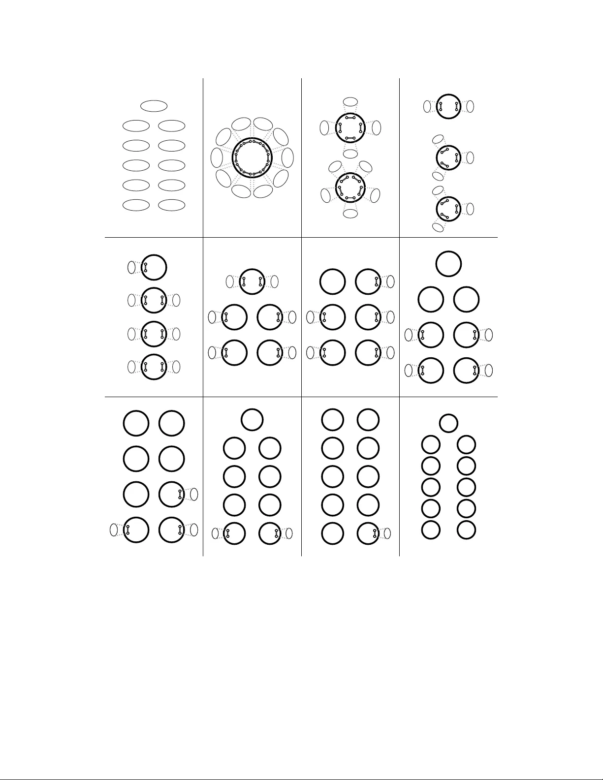
For $r \ge 2$ and a graph $G$, let $α_{r}(G)$ be the maximum number of vertices in a $K_r$-free subgraph of $G$. We investigate the value $α_{r}(G)$ when $G$ is the random graph $G \sim G_{n, 1/2}$ and discover the following phenomenon: with high pro…
Authors: Tom Bohman, Marcus Michelen, Dhruv Mubayi
The largest K r -free set of v ertices in a random graph T om Bohman ∗ Marcus Mic helen † Dhruv Muba yi ‡ Abstract F or r ≥ 2 and a graph G , let α r ( G ) b e the maximum n umber of vertices in a K r -free subgraph of G . W e in vestigate the v alue α r ( G ) when G is the random graph G ∼ G n, 1 / 2 and disco ver the follo wing phenomenon: with high probability , α r ( G ) lies in an interv al of constan t length that v aries in a non-monotonic fashion from 1 to ⌊ r / 2 ⌋ + 1 depending on the v alue of n . The sp ecial case r = 2 corresp onds to the indep endence n umber of random graphs which is w ell-known to ha ve tw o-p oin t concentration; our results therefore extend and generalize this basic fact in random graph theory , showing more complicated b eha vior when r > 2. W e also pro ve similar results where K r is replaced by any color critical graph lik e C 5 . 1 In tro duction Consider the binomial random graph G n, 1 / 2 and let α ( G n, 1 / 2 ) b e its indep endenc e numb er , i.e. the size of the largest indep enden t set of G . In the 1970’s, classical works of Bollob´ as and Erd˝ os [ 6 ] and Matula [ 15 ] indep enden tly show ed that α ( G n, 1 / 2 ) is concen trated on at most tw o v alues meaning that there is a deterministic function f ( n ) so that lim n →∞ P ( α ( G n, 1 / 2 ) ∈ { f ( n ) , f ( n ) + 1 } ) = 1 . In fact, the works of Bollob´ as-Erd˝ os and Matula [ 6 , 15 ] imply that for a typical in teger n , α ( G n, 1 / 2 ) is concentrated on a single v alue, meaning that for most n w e hav e α ( G n, 1 / 2 ) = f ( n ) with high probabilit y . Similar results are also known for G ∼ G n,p as long as p is not sufficiently small in terms of n [ 11 , 8 , 5 , 4 ]. One may interpret an indep enden t set as simply a subset of G n, 1 / 2 that a voids the presence of an edge, i.e. a clique on t wo vertices. With this in mind, for a graph G , define α r ( G ) to b e the maximum num b er of vertices in an induced subgraph of G that do es not con tain a copy of K r , the clique on r v ertices. W e note in passing that instead of vertices one can ∗ Departmen t of Mathematical Science, Carnegie Mellon Universit y . Email: tbohman@math.cmu.edu. Researc h partially supported by NSF Aw ard DMS-2246907 † Departmen t of Mathematics, Northw estern Universit y . Email: mic helen@northw estern.edu. Research partially supp orted by NSF a wards DMS-2336788 and DMS-2246624 ‡ Departmen t of Mathematics, Statistics and Computer Science, Universit y of Illinois, Chicago, IL 60607. Email: m ubayi@uic.edu. Research partially supp orted b y NSF Award DMS-2153576. 1 also consider the maximum num b er of edges in a subgraph of G n,p that contains no copy of K r ; this problem, p osed b y Babai-Simono vits-Sp encer [ 2 ] in 1990, has a long and storied history . Some of the influential results here are due to Conlon-Gow ers [ 7 ], Schac h t [ 18 ], and DeMarco-Kahn [ 9 ]. In analogy with the indep endence n umber, we study the problem of concen tration of the random quan tity α r ( G n, 1 / 2 ). In particular, does t wo-point concen tration still hold for α r ( G n, 1 / 2 )? P erhaps surprisingly , one consequence of our w ork is that t wo-point concen tration holds for r = 2 , 3 and fails for r ≥ 4. W e sho w that for each fixed 1 r ≥ 2 we hav e that α r ( G n, 1 / 2 ) lies in an in terv al of constant length that v aries in a non-monotonic fashion from 1 to ⌊ r / 2 ⌋ + 1 dep ending on the sp ecific v alue of n . This phenomenon is closely tied to the fact that as n v aries, the n umber of indep enden t sets of size α ( G n, 1 / 2 ) can b e as small as O (1) or as large as n 1+ o (1) dep ending on n . This non-monotonicity is also what driv es the c hanging exponent of the concentration window for the c hromatic nu mber of G n, 1 / 2 in the w ork of Hec kel [ 12 ] (see also Hec kel-Riordan [ 13 ] for a precise conjecture). As is the case with the indep endence n umber, for a t ypical v alue of n , α r ( G n, 1 / 2 ) is concen trated on a single v alue; when not concentrated on a single v alue, the size of the interv al can take on m ultiple v alues for a given r that dep end on divisibility properties of r . F or instance, in the case of, sa y , r = 1001, there will b e v alues of n for whic h α r ( G n, 1 / 2 ) is concentrated on exactly 2 v alues, some where it is concen trated on exactly 501 v alues, some where it is concentrated on exactly 84 v alues. In fact, w e will sho w that in the case of r = 1001, as n v aries α r ( G n, 1 / 2 ) is concentrated on in terv als of length { 1 , 2 , 3 , 4 , 5 , 6 , 8 , 11 , 12 , 15 , 18 , 25 , 35 , 51 , 84 , 168 , 501 } . The pattern of what in terv als of concen tration o ccurs is non-monotone, with alwa ys going to 1 b efore a larger v alue. In particular, we first get 1 point concentration, then 2 point concentration; it alternates b et ween 1-p oin t and 2-point concentration 34 times b efore seeing 3-p oin t. F urther, the in terv al can shrink ev en aside from going bac k to 1 point. In the case of r = 1001 w e ha v e a stretc h where w e see 3-point then 1-p oin t, 2-p oin t, 1-p oin t, 3-point, 1-p oint, 2-p oin t. In general the pattern is complicated, but is fully described b y Theorem 2 . Our most general main theorem is Theorem 1 which describ es a criterion for witnessing b oth upp er and lo wer b ounds of α r ( G n, 1 / 2 ) along with a statement identifying Poissonian b eha vior for these witnesses; w e use Theorem 1 to deduce a complete description of the interv als of concentration in Theorem 2 . Before jumping in to describ e this general case, we describe the story for the case of r = 3, i.e. the largest triangle-free s ubgraph of G n, 1 / 2 . W e describ e the case of triangles along with a heuristic description of what happ ens for larger cliques in Section 1.1 , state our more general theorem in Section 1.2 and describ e the in terv als of concentration in Section 1.3 . Finally , w e describ e some sligh tly coarser results for when a voiding c olor critic al graphs other than K r in Section 1.4 . 1 Our main result Theorem 1 will in fact apply for r = o (log log n/ log log log n ). 2 1.1 The case of triangles and a heuristic description for larger cliques The exp ected num b er of triangle-free subgraphs of size k in G n, 1 / 2 is precisely giv en b y N 3 ( k ) n k 2 − ( k 2 ) where N 3 ( k ) is the n umber of triangle-free graphs on v ertex set [ k ]. A classical theorem of Erd˝ os- Kleitman-Rothsc hild [ 10 ] states that almost all triangle-free graphs are bipartite graphs. With this in mind, one migh t hop e that rather than searching for a large triangle-free graph in G n, 1 / 2 , w e migh t b e able to simply searc h for a large bipartite graph. In terestingly , it turns out that this is not precisely the case. Supp ose we are in the case where for some v alue of n , the independence num b er is k with high probabilit y . As n increases, the indep endence num b er will ev en tually b e k + 1 with high probabilit y . As this transition occurs, before seeing gen uine indep enden t sets of size k + 1, we will b egin to see some num b er of sets of k + 1 containing only 1 edge. W e call suc h an edge a defe ct . If one considers an indep enden t set of size k and a ( k + 1)-set with a defect, it will not b e to o common that the union of these t wo sets induces a triangle free graph—indeed one can compute that the probabilit y a given k -set and ( k + 1)-set with a defect com bine to give a triangle-free graph is (3 / 4) − k —but despite this probability being so small, it turns out that by the time there is a ( k + 1)-set with a defect there are enough indep enden t sets of size k that in fact it is lik ely that a triangle-free graph of size 2 k + 1 occurs. In particular, if we define Y k to be the n umber of independent sets of size k and Z k, 1 to b e the n umber of k -sets of v ertices that con tain exactly 1 edge, then Theorem 1 implies that P ( α 3 ( G n, 1 / 2 ) ≥ 2 k + 1) = P ( Z k +1 , 1 ≥ 1) + o (1) P ( α 3 ( G n, 1 / 2 ) ≥ 2 k ) = P ( Y k ≥ 2) + o (1) for each k chosen so that n − O (1) ≤ E [ Y k ] ≤ n O (1) . F urther, each of Z k, 1 and Y k b eha v e like P oisson random v ariables provided their mean is, say , no more than n 1 / 4 . T o describ e the interv als of concen tration, for a small parameter ε = o (1) w e may define a k = min { n : E [ Y k ] ≥ ε − 1 } b k, 1 = min { n : E [ Z k +1 , 1 ] ≥ ε } , c k, 1 = min n : E [ Z k +1 , 1 ] ≥ ε − 1 , b k, 2 = min { n : E [ Y k +1 ] ≥ ε } , c k, 2 = min n : E [ Y k +1 ] ≥ ε − 1 . Then α 3 ( G n, 1 / 2 ) ∈ I n with high probabilit y where I n is the in terv al I n = { 2 k } if a k ≤ n < b k, 1 { 2 k , 2 k + 1 } if b k, 1 ≤ n < c k, 1 { 2 k + 1 } if c k, 1 ≤ n < b k, 2 { 2 k + 1 , 2 k + 2 } if b k, 2 ≤ n < c k, 2 = a k +1 . F or larger r , w e recall that classical works of Erd˝ os-Kleitman-Rothschild [ 10 ] and Kolaitis-Pr¨ omel- Rothsc hild [ 14 ] sho w that almost ev ery K r +1 -free graph is r -partite. As n v aries, we will see that 3 for most v alues of n the subgraphs that realize α r +1 ( G n, 1 / 2 ) are in fact r -partite graphs. As n increases and w e transition from having indep endence num b er k to independence n umber k + 1, there will be v ertex sets of size k + 1 that hav e a small n umber of edges. As in the case of triangles, w e refer to these edges as defe cts in potential indep enden t sets. It turns out that w e can incorporate these ( k + 1)-sets with few defects in to K r +1 -free subgraphs. W e sho w that this can be done by “co vering” eac h individual defect with an independent set of size k , where a k -set A c overs a defect e if there is no copy of K 3 that consists of e and a vertex in A . The p oin t of this definition is that an y cop y of K r +1 that con tains a defect from a ( k + 1)-set cannot hav e an y v ertex in a k -set that co vers the defect; this allo ws us to include b oth these sets in a K r +1 -free subgraph. It turns out that for n in this regime we can form a maxim um K r +1 -free subgraph of G n, 1 / 2 b y iden tifying disjoin t sets A 1 , . . . , A r where each set A i is either an indep enden t set of size k or a set of size k + 1 with a small n umber of defects with the prop ert y that each defect is co vered by an indep enden t set of size k in the collection. It will also b e the case that eac h k -set cov ers only one defect. W e sho w that in this regime X is equal to the maximum n um b er of vertices in such a structure. W e do not show that all K r +1 -free subgraphs of maxim um size hav e this form; indeed, in some cases differen t—but closely related—maximum structures are also p ossible. 1.2 Concen tration via P oissonian statistics W e no w prepare to describ e our main result. As a typical K r -free graph is ( r − 1)-partite it will b e more notationally con v enient to work with K r +1 -free subgraphs. F or r = o (log log n/ log log log n ), set X = α r +1 ( G n, 1 / 2 ) . In analogy with the case of triangles, define Y k = n umber of indep enden t sets of size k Z k,i = n umber of k -sets of v ertices that con tain exactly i edges . F or eac h j ∈ { 1 , . . . , r } define µ j = r − j j = r j − 1 and ξ j = j ( µ j + 2) − r. Note that w e hav e 1 ≤ ξ j ≤ j . Just as we were occasionally able to form a triangle-free graph b y combining an indep enden t set of size k with a k + 1-set with a single defect, w e will see that there are v alues for n in the regime where E [ Y k +1 ] go es to zero sufficiently slowly (to b e precise, n in the regime defined b y E [ Y k +1 ] ≈ (log n ) − 2 µ j ) for whic h we can form a K r +1 -free subgraph in G n, 1 / 2 with k r + j vertices by using ξ j man y ( k + 1)-sets that ha ve µ j defects each and j − ξ j man y ( k + 1)-sets with µ j + 1 defects each. Each defect in this structure is cov ered by an indep enden t set of size k , and it follows that the total n umber of k -sets and ( k + 1)-sets in volv ed in the structure is ξ j ( µ j + 1) + ( j − ξ j )( µ j + 2) = j ( µ j + 2) − ξ j = r . Note that we cannot form such a structure with few er than ξ j man y ( k + 1)-sets with µ j defects eac h as this w ould require to o man y k -sets to cov er all of the defects. Of course, in order for suc h 4 a structure to appear n must b e large enough for ( k + 1)-sets with µ j defects to app ear in G n, 1 / 2 . Note that as n increases the smallest num b er of defects in a ( k + 1)-set decreases. Our main result is that structures of the t yp e discussed ab o ve go v ern the ev olution of X ; the app earance of these structures is in turn go verned b y the n umber of ( k + 1)-sets with few defects; and the n umber of ( k + 1)-sets with a particular n umber of defects has the Poissonian statistics that we w ould an ticipate. Theorem 1. L et k = 2 log 2 n + O (log log n ) , r = o (log log n/ log log log n ) . Then, for n sufficiently lar ge and j ∈ { 1 , . . . , r } we have P ( X ≥ kr + j ) − P ( Z k +1 ,µ j ≥ ξ j ) ≤ (log n ) − 1 / 2 . F or λ = E [ Z k +1 ,µ j ] ≤ n 1 / 4 we also have P (P oiss( λ ) ≥ ξ j ) − P ( Z k +1 ,µ j ≥ ξ j ) ≤ n − 1 / 4 . See Figure 1 for a depiction of some of the structures that gov ern the evolution of α r +1 ( G n, 1 / 2 ) in the case r = 11. 1.3 The in terv al of concen tration for K r +1 W e now deduce the extent of concentration of α r +1 ( G n, 1 / 2 ) for fixed r directly from Theorem 1 . Implicit in Theorem 1 is that for each j ∈ { 1 , 2 , . . . , r } such that µ j = µ j +1 there is an interv al in n in whic h α r +1 ( G n, 1 / 2 ) is lik ely to b e equal to r k + j . In order to mak e this precise, we define a sequence of v alues of n , m uch lik e we did for the r = 3 case in Section 1.1 . W e b egin b y defining the p oin t at which it is likely that there is a K r +1 -free set of vertices in G n, 1 / 2 that consists of r indep enden t sets of size k . Note that E [ Y k ] = n k 2 − ( k 2 ) . Set 2 ε = ε ( k ) = 1 / log k and define a k = min n : E [ Y k ] ≥ ε − 1 . First, let us observ e that the sequence a k is exponential in k . W e begin b y noting that the bound n k ≤ ( ne/k ) k implies a k > ( k /e )2 ( k − 1) / 2 . Next observe that if n > 2 ( k − 1) / 2 , then E [ Y k ] = ne k 2 − k − 1 2 k e O ( k 2 / 2 k − 1 )+ O (log k ) . This implies a k = (1 + o k (1)) k e 2 k − 1 2 and a k +1 = ( √ 2 + o k (1)) a k . W e will see that for the ma jorit y of the v alues for n in the in terv al [ a k , a k +1 ) w e hav e X = r k with probabilit y at least 1 − O ( ε ). Then, as n approac hes a k +1 , the structure of a maxim um K r +1 -free subgraph go es through a series of transitions that interpolate b et ween a subgraph of a T ur´ an graph 2 Note the c hoice of this particular function is made for con venience. Any ε = o k (1) suffices. 5 J J J J J J Figure 1: These images depict likely maxim um induced subgraphs of G n, 1 / 2 not containing K 12 at differen t points in the evolution of G n, 1 / 2 (where we view n as growing and the edge probability is fixed at 1 / 2). The blac k circles represen t sets of k + 1 v ertices that ha ve some num b er of defects, whic h are the gray edges. The gray ov als are independent sets of size k , and the dotted lines indicate whic h k -sets cov er whic h defects. Note that w e ha ve µ 1 = 10 , ξ 1 = 1; µ 2 = 4 , ξ 2 = 1; µ 3 = 2 , ξ 3 = 1; µ 4 = 1 , ξ 4 = 1; µ 5 = 1 , ξ 5 = 4 and J = { 1 , 2 , 3 , 5 , 11 } . W e placed a J for sets whose size lies in J mod 11. These sizes form the endp oin ts of the in terv als of concentration of X . 6 on k r vertices and a subgraph of a T ur´ an graph on ( k + 1) r vertices. In order to capture this b eha vior, we need some additional definitions. F or a k ≤ n < a k +1 define µ = µ ( n ) = min i : E [ Z k +1 ,i ] > ε − 1 , and note that µ ( n + 1) ≤ µ ( n ). Recall that w e define µ j = r − j j = r j − 1 , and b y Theorem 1 we exp ect to ha ve K r +1 -free subgraphs with k r + j vertices with some sig- nifican t probability for those j such that µ ≤ µ j . Note that the quan tity µ ( n ) decreases from Θ(log n/ log log n ) to 0 as n increases from a k to a k +1 (see F act 6 that app ears later in the pap er for the detailed calculations that imply this). Thus, for the v ast ma jorit y of the in terv al there is no impro vemen t relativ e to the b ound α r +1 ( G n, 1 / 2 ) ≥ k r , since sets of size k + 1 will hav e to o man y defects to be included in our K r +1 -free subgraph. Then, as n approac hes a k +1 , w e see v alues of µ ( n ) that equal µ j for 1 ≤ j ≤ r , and it is here that we see increases in α r +1 ( G n, 1 / 2 ). There is a series of c hanges in this v alue as µ ( n ) decreases whic h we now describ e. Let J b e the set of integers j ∈ { 1 , . . . , r } such that µ j = µ j +1 (where w e set µ r +1 = − 1) and set s = |J | . F or example, if r = 11, then J = { 1 , 2 , 3 , 5 , 11 } and if r = 23, then J = { 1 , 2 , 3 , 4 , 5 , 7 , 11 , 23 } . W rite J = { j i : i ∈ [ s ] } = { 1 = j 1 < j 2 < · · · < j s = r } , and for eac h i ∈ [ s ] set b k,i = min n n : E [ Z k +1 ,µ j i ] ≥ ε o , c k,i = min n n : E [ Z k +1 ,µ j i ] ≥ ε − 1 o , and note that c k,s = a k +1 . Observ e that these definitions imply the follo wing chain of inequalities. The calculations needed to justify these inequalities ma y be found in Theorem 6 . a k ≤ b k, 1 ≤ c k, 1 ≤ b k, 2 ≤ c k, 2 ≤ · · · ≤ b k,s − 1 ≤ c k,s − 1 ≤ b k,s ≤ c k,s = a k +1 . W e are no w ready to define the interv als on which X is concentrated. Set j 0 = 0 and c 0 = a k . Define I n = { k r + j i − 1 } if c k,i − 1 ≤ n < b k,i and 1 ≤ i ≤ s { k r + j i − 1 , . . . , k r + j i } if b k,i ≤ n < c k,i and 1 ≤ i ≤ s In other w ords, if n ∈ [ b k,j i , b k,j i +1 ), then I n is either { k r + j i − 1 , . . . , k r + j i } or { k r + j i } according to whether n < c k,j i or n ≥ c k,j i . Example. If r = 11, then J = { 1 , 2 , 3 , 5 , 11 } , s = 5, and j 1 = 1 , j 2 = 2 , j 3 = 3 , j 4 = 5 , j 5 = 11. 7 Consequen tly , I n = { 11 k } if a k = c k, 0 ≤ n < b k, 1 { 11 k , 11 k + 1 } if b k, 1 ≤ n < c k, 1 { 11 k + 1 } if c k, 1 ≤ n < b k, 2 { 11 k + 1 , 11 k + 2 } if b k, 2 ≤ n < c k, 2 { 11 k + 2 } if c k, 2 ≤ n < b k, 3 { 11 k + 2 , 11 k + 3 } if b k, 3 ≤ n < c k, 3 { 11 k + 3 } if c k, 3 ≤ n < b k, 4 { 11 k + 3 , 11 k + 4 , 11 k + 5 } if b k, 4 ≤ n < c k, 4 { 11 k + 5 } if c k, 4 ≤ n < b k, 5 { 11 k + 5 , . . . , 11( k + 1) } if b k, 5 ≤ n < c k, 5 = a k +1 . See Figure 1 for a depiction of some of the structures in volv ed in eac h step here. With this preparation, we no w state our result regarding the concen tration of α r +1 ( G n, 1 / 2 ). Theorem 2. Fix r ≥ 1 . Then whp α r +1 ( G n, 1 / 2 ) ∈ I n . Pr o of. Theorem 2 will follo w immediately from Theorem 1 . Indeed, setting j = j i − 1 + 1 w e ha ve µ j = µ j i and n < b k,i = ⇒ E [ Z k +1 ,µ j i ] < ε = ⇒ E [ Z k +1 ,µ j ] < ε = ⇒ P ( X > rk + j i − 1 ) = P ( X ≥ rk + j ) ≤ P (P oiss( ε ) ≥ 1) + o n (1) = 1 − e − ε + o n (1) = O ( ε ) . And, for k sufficien tly large we ha ve n ≥ c k,i = ⇒ E [ Z k +1 ,µ j i ] > 1 /ε = ⇒ P ( X ≥ r k + j i ) ≥ P (P oiss(1 /ε ) ≥ r ) − o n (1) = 1 − (1 /ε ) r r ! e − 1 /ε − o n (1) = 1 − o k (1) . Consequen tly , the implications abov e imply that if c k,i − 1 ≤ n < b k,i , then P ( X = k r + j i − 1 ) = P ( X ≥ k r + j i − 1 ) − P ( X > kr + j i − 1 ) ≥ 1 − o k (1) − O ( ε ) and if b k,i ≤ n < c k,i , then, since c k,i − 1 ≤ b k,i ≤ n < c k,i ≤ b k,i +1 , we hav e P ( X > kr + j i ) = O ( ε ) and P ( X < k r + j i − 1 ) = o k (1) . The proof of Theorem 1 is split into upp er and lo wer b ounds. Sho wing a lo w er b ound on X ≥ kr + j will b e fairly simple: we sho w that one can take ξ j man y ( k + 1)-sets with µ j defects, j − ξ j man y ( k + 1)-sets with µ j + 1 defects, and r − j man y k indep enden t sets and com bine them to get a K r +1 - free set on k r + j vertices. The upper b ound is more delicate. One imp ortan t tool in the pro of of 8 the upp er b ound is a result of Balogh and Samotij [ 3 ] which coun ts the num b er of K r +1 -free graphs on k v ertices that are far from b eing r -partite. Their argumen t is an application of an efficien t h yp ergraph con tainer lemma (see Theorem 17 ) and can be view ed as a generalization and refinemen t of the classical works of Erd˝ os-Kleitman-Rothsc hild [ 10 ] and Kolaitis-Pr¨ omel-Rothschild [ 14 ] who sho wed that almost all K r +1 -free graphs are r -partite. 1.4 Color-critical graphs and other prop erties Rather than lo oking only at the largest K r -free subgraph, we can similarly examine the largest F -free graph, where we use F -free to mean that there is no (not necessarily induced) subgraph isomorphic to F . With this in mind, define α F ( G ) to b e the size of the largest F -free subgraph of G . Sa y that a graph is r - c olor-critic al (henceforth r - critic al ) if χ ( F ) = r + 1 and F contains an edge whose deletion reduces its c hromatic n umber to r . F or example, C 5 is 2-critical. While we are not able to deduce as refined a statemen t for α F for color-critical graphs, we are able to sho w concen tration on an in terv al of size at most r +1. Theorem 3. Fix r ≥ 2 and an r -critic al gr aph F . Ther e is a se quenc e m n so that with high pr ob ability α F ( G n, 1 / 2 ) ∈ [ m n − r, m n ] . R emark 4 . The proof of Theorem 3 yields a somewhat explicit choice of m n . Let m 0 b e the smallest in teger so that the expected num b er of F -free graphs in G n, 1 / 2 whose v ertex set has size m 0 is at most 1. Then w e tak e either m n = m 0 − 1 or m n = m 0 − 2 dep ending on the exp ected n um b er of F -free subgraphs of size m 0 . As an example, Theorem 3 implies that whp α C 5 ( G n, 1 / 2 ) ∈ { m n − 2 , m n − 1 , m n } . The pro of of Theorem 3 is muc h simpler: the upp er b ound is given by using a theorem of Pr¨ omel and Steger en umerating suc h graphs along with a basic union bound; for the low er b ound, the theorem of Pr¨ omel and Steger will essen tially say that the num b er of such graphs is the same as the num b er of r -partite graphs, and so w e will find an r -partite graph using the same ideas as in the pro of of Theorem 1 . More generally , a pr op erty P of graphs is a class of graphs closed under isomorphism. Given a prop ert y P and a graph G , let α P ( G ) b e the maximum num b er of vertices in an induced subgraph of G that is isomorphic to some member of P . A graph property P is monotone (resp ectiv ely her e ditary ) if ev ery (induced) subgraph of a graph with property P also has prop ert y P . F or instance, being a bipartite graph or b eing a triangle-free graph is monotone, while b eing p erfect or c hordal is hereditary . T o every monotone (hereditary) prop ert y P , there exists a collection F of graphs such that G ∈ P if and only if every (induced) subgraph of G is not isomorphic to any mem b er of F . W e end with the follo wing problem, whic h asks if for ev ery monotone or hereditary prop ert y there is concentration on a constan t-length in terv al. 9 Problem 5. L et P b e a monotone or her e ditary pr op erty. Do es ther e exist a p ositive inte ger R = R P such that with high pr ob ability α P ( G n, 1 / 2 ) lies in an interval of length at most R ? W e b eliev e this is true for all prop erties P for whic h the n umber of graphs on n v ertices in P is 2 Ω( n 2 ) . 2 Preparations for pro of of Theorem 1 W e now b egin discussing v arious ingredients needed for our proof of Theorem 1 . Throughout the rest of the paper w e will assume that n is sufficien tly large. W e will first compute v arious relev ant scales and then imp ort a few useful to ols suc h as Janson’s inequalit y and a consequence of the Stein-Chen metho d on P oisson appro ximation. 2.1 Useful asymptotics Recall that Z k,i is the num b er of k -sets with exactly i edges and Y k = Z k, 0 is the num b er of indep enden t sets of size k . W e start with a basic calculation for understanding the scales at pla y . F act 6. We have E [ Y k ] = n O (1) if and only if k = 2 log 2 n − 2 log 2 log 2 n + O (1) . If k = 2 log 2 n + O (log log n ) then we also have E [ Y k +1 ] / E [ Y k ] = n − 1+ o (1) . If we further have i = O (log log n ) then E [ Z k,i ] = k 2 i (1+ o (1)) E [ Y k ] Pr o of. W rite k = 2 log 2 n − 2 log 2 log 2 n − t and compute E [ Y k ] = n k 2 − ( k 2 ) = exp 2 ((1 + o (1)) k [log 2 n − log 2 k − k/ 2 + O (1)]) = n (1+ o (1)) t + O (1) . The second assertion is similar. F or the third assertion, note that E [ Z k,i ] = n k k 2 i 2 − ( k 2 ) = k 2 i (1+ o (1)) E [ Y k ] completing the proof. W e will also make frequent use of a second momen t-type calculation: F act 7. If k = 2 log 2 n + O (log log n ) then n k k − 1 X j =1 k j n − k k − j 2 − 2 ( k 2 ) + ( j 2 ) ≤ n − 1+ o (1) ( E [ Y k ] 2 + E [ Y k ]) . 10 Pr o of. F or j ∈ [ k − 1], write C j = k j n − k k − j 2 ( j 2 ) so that n k k − 1 X j =1 k j n − k k − j 2 − 2 ( k 2 ) + ( j 2 ) = n k 2 − 2 ( k 2 ) k − 1 X j =1 C j . Bound C j +1 C j = k − j j + 1 n − k k − j − 1 n − k k − j 2 j ≤ log 3 n · n − 1 2 j . Ab o v e we added an extra factor of log n to absorb all implicit constan ts. F or 2 ≤ j ≤ (3 / 4) k w e then hav e C j C 1 = j − 1 Y i =1 C i +1 C i ≲ log 3 n · 2 j / 2 n ! j − 1 ≤ n − 1+ o (1) . Similarly b ound C k − ( j +1) C k − j ≤ log 3 n · n · 2 − ( k − j ) . F or 2 ≤ k − j ≤ (3 / 4) k we then ha ve C k − j C k − 1 ≤ n − 1+ o (1) . This implies n k k − 1 X j =1 k j n − k k − j 2 − 2 ( k 2 ) + ( j 2 ) ≤ (1 + o (1)) n k 2 − 2 ( k 2 ) ( C 1 + C k − 1 ) = (1 + o (1)) n k 2 − 2 ( k 2 ) k n − k k − 1 + k ( n − k )2 ( k − 1 2 ) = n − 1+ o (1) ( E [ Y k ] 2 + E [ Y k ]) . 2.2 P oisson Appro ximation Define P oiss( λ ) to be the P oisson distribution of mean λ and set d TV ( X , Poiss( λ )) to b e the total v ariation distance to the P oisson of mean λ , i.e. d TV ( X , Poiss( λ )) = X k ≥ 0 P ( X = k ) − e − λ λ k k ! . The Stein-Chen metho d will allow us to sho w that the num b er of copies of certain subgraphs will b e appro ximately P oisson. W e use the following simplified v ersion from [ 1 , Thm. 1] Theorem 8. F or α ∈ A , let X α b e a Bernoul li r andom variable and set p α = E [ X α ] = P ( X α = 1) . L et W = P α ∈A X α . F or e ach α , let B α = { β : X α and X β ar e not indep endent } . Then d TV ( W , Poiss( E [ W ])) ≤ 2 X α ∈A X β ∈ B α p α p β + X α ∈A X β ∈ B α \ α E [ X α X β ] . 11 Our main use of Theorem 8 is to show P oissonian statistics for Z k,i . Lemma 9. If k = 2 log 2 n + O (log log n ) and i = O (log n log n ) then d TV ( Z k,i , P oiss( E [ Z k,i ])) ≤ n − 1+ o (1) ( E [ Z k,i ] 2 + E [ Z k,i ]) . Pr o of. Let λ = E [ Z k,i ] = E [ Y k ] n o (1) . Set A = [ n ] k to b e the collection of k sets of [ n ] and for eac h α ∈ A set X α to b e the indicator that α has exactly i edges; note that Z k,i = P α ∈A X α . F urther, note that p α is constant o ver all α and we ha ve p α = λ/ n k = ( k 2 ) i 2 − ( k 2 ) . Note that w e ha ve ( k 2 ) i = n o (1) . F or each α , we hav e that B α is the collection of sets that o verlap with α in at least 2 v ertices. W e can then b ound X α ∈A X β ∈ B α \ α E [ X α X β ] ≤ n o (1) n k k − 1 X j =2 k j n − k k − j 2 − 2 ( k 2 ) + ( j 2 ) ≤ n − 1+ o (1) ( E [ Z k,i ] 2 + E [ Z k,i ]) b y F act 7 . A similar argumen t sho ws X α ∈A X β ∈ B α p α p β ≤ n − 1+ o (1) ( E [ Z k,i ] 2 + E [ Z k,i ]) and so Theorem 8 completes the pro of. 2.3 Janson’s inequalit y W e make use of not only the classical Janson’s inequalit y but also a generalization due to Riordan and W arnk e [ 17 ]. The set-up for our application of these inequalities is as follo ws. Let S be a finite set, consider the probabilit y space on the Ω = { 0 , 1 } S giv en b y the product measure, and let I b e the collection of all decreasing even ts in Ω. This implies that for all A ∩ B ∈ I , we ha ve P ( A ∩ B ) ≥ P ( A ) P ( B ), A ∪ B ∈ I , and A ∪ B ∈ I . Given A 1 , . . . , A k ∈ I we let I i b e the indicator random v ariable for the even t A i and set X = k X i =1 I i and ∆ = X i X j ∼ i P ( A i ∩ A j ) where we write i ∼ j if i = j and A i and A j are dep enden t. Theorem 10 (Janson; Riordan and W arnk e) . Under the c onditions ab ove, for any 0 ≤ t ≤ µ w e have P ( X ≤ E [ X ] − t ) ≤ e − t 2 2( µ +∆) . Note that w e reco ver Janson’s inequalit y b y sp ecifying a collection of sets B 1 , B 2 . . . , B k ⊂ Ω and letting the ev ent A i b e the even t no elemen t of B i app ears. 12 3 The lo wer b ound: co v ering defects with indep enden t sets Our goal is to prov e the follo wing that giv es the low er b ound for Theorem 1 . Recall that µ j = ⌊ ( r − j ) /j ⌋ and ξ j = ( µ j + 2) j − r . Lemma 11. L et n b e sufficiently lar ge and supp ose k = 2 log 2 n − 2 log 2 log n + O (1) , r = o (log log n ) . If 0 < j ≤ r then P ( X ≥ kr + j ) ≥ P ( Z k +1 ,µ j ≥ ξ j ) − 1 log n . W e begin b y noting that we ma y assume 1 2 log n < E [ Z k +1 ,µ j ] < log 4 r n (1) Indeed, if E [ Z k +1 ,µ j ] ≤ (2 log n ) − 1 then, by Theorem 9 w e ha ve P ( Z k +1 ,µ j ≥ ξ j ) ≤ P ( Z k +1 ,µ j ≥ 1) ≤ n − 1+ o (1) + 1 − e − E [ Z k +1 ,µ j ] ≤ 1 log n , and the conclusion of Theorem 11 is trivial. T o see the upp er b ound, note that we ha ve E [ Z k +1 ,i +1 ] E [ Z k +1 ,i ] = k 2 − i i + 1 ≤ log 4 n. (2) It follo ws that if E [ Z k +1 ,µ j ] ≥ log 4 r n then E [ Z k +1 , 0 ] = E [ Y k +1 ] > log 4 n . W e may assume E [ Y k +1 ] ≤ n 1 / 4 b y simply restricting our attention to a subset of the vertex set. Then Theorem 9 implies that it is likely that there are at r indep enden t sets of size k + 1, and a first momen t calculation using Theorem 7 sho ws that these indep enden t sets are disjoint whp. So w e hav e a K r +1 -free set b y taking the union of r pairwise-disjoin t indep enden t sets of size k + 1; to be precise, w e ha ve P ( X ≥ kr + j ) ≥ P ( X ≥ ( k + 1) r ) ≥ 1 − n − 1 / 2+ o (1) . As E [ Z k +1 ,i ] ≥ log 4 n =: λ implies P ( Z k +1 ,i ≥ r ) ≥ 1 − r − 1 X ℓ =0 e − λ λ ℓ ℓ ! ≥ 1 − e − (log n ) 2 + O ((log log n ) 2 ) , this b ound suffices to establish the conclusion of Theorem 11 in this case. Note that assumption ( 1 ) implies E [ Y k ] = n 1+ o (1) . No w, for eac h k and i , define Z k,i to be the collection of k -sets of [ n ] that induced exactly i edges so that Z k,i = |Z k,i | . Similarly define Y k = Z k, 0 to be the collection of indep enden t sets of size k . W e will show that elemen ts of Z k,i ∪ Z k,i +1 are pairwise disjoint in the relev ant regime. Define the “bad” even t B 1 via B 1 = {∃ S 1 , S 2 ∈ Z k +1 ,i ∪ Z k +1 ,i +1 , S 1 = S 2 , S 1 ∩ S 2 = ∅} . A simple union b ound will handle P ( B 1 ): 13 F act 12. F or k = 2 log 2 n + O (log log n ) and i = o (log n/ log log n ) we have P ( B 1 ) ≤ n − 1+ o (1) ( E [ Z k +1 ,i ] 2 + E [ Z k +1 ,i ]) . Pr o of. As i = o (log n/ log log n ), w e ha ve k i = n o (1) . W e union bound ov er all possible c hoices and use Theorem 7 to bound P ( B 1 ) ≤ n o (1) n k + 1 k X j =1 k + 1 j n − k − 1 k + 1 − j 2 − 2 ( k +1 2 ) + ( j 2 ) ≤ n − 1+ o (1) ( E [ Z k +1 ,i ] 2 + E [ Z k +1 ,i ]) . F or S ∈ Z k,i let D ( S ) denote the set of defects in S . Recall that an indep enden t set T ∈ Y k c overs an edge e if there is no triangle consisting of a vertex in T together with e . W e prov e that each defect is cov ered b y man y independent sets of size k . Set C ( e ) = { T ∈ Y k : T co vers e } . Define the bad even ts B 2 and B 3 via B 2 := n ∃ S ∈ Z k +1 ,i ∪ Z k +1 ,i +1 , e ∈ D ( S ) : |C ( e ) | ≤ (3 / 4) k E [ Y k ] / 2 o B 3 := {∃ S ∈ Z k +1 ,i ∪ Z k +1 ,i +1 , e ∈ D ( S ) , T 1 , T 2 ∈ C ( e ) : T 1 ∩ T 2 = ∅ , T 1 = T 2 } . Lemma 13. Supp ose that E [ Y k ] ∈ [ n 5 / 6 , n 6 / 5 ] . Then for i = O (log log n ) we have P ( B 2 ) ≤ n − 1 / 100 and P ( B 3 ) ≤ n − 1 / 100 . Pr o of. Let S ∈ Z k +1 ,i ∪ Z k +1 ,i +1 and e ∈ D ( S ). W e begin with a union b ound: P ( B 2 ) ≤ ( i E [ Z k +1 ,i ] + ( i + 1) E [ Z k +1 ,i +1 ]) P n − ( k +1) |C ( e ) | ≤ (3 / 4) k E [ Y ′ k ] / 2 (3) where w e write P n − ( k +1) for the distribution of the random graph on V 2 \ S 2 , e ∈ S and Y ′ k is the n umber of indep enden t sets of size k that do not intersect S . T o handle this probabilit y , we will sho w by the second moment metho d that the n umber of in- dep enden t sets that co ver the disjoint edge e is near its mean. Define N = n − ( k + 1). Set X S = |{ T ∈ C ( e ) : S ∩ T = ∅}| and note E [ X S ] = (3 / 4) k N k 2 − ( k 2 ) = (1 + o (1))(3 / 4) k E [ Y ′ k ] . (4) W e also can b ound V ar[ X S ] − E [ X S ] ≤ N k k − 1 X j =1 k j N − k k − j 2 − 2 ( k 2 ) + ( j 2 ) (3 / 4) 2 k − j = N − 1+ o (1) E [ X S ] 2 + E [ X S ] 14 where the second line is by adapting Theorem 7 and we recall E [ X S ] = (1 + o (1))(3 / 4) k E [ Y ′ k ] by ( 4 ). By Chebyshev’s inequalit y , we then see P ( X S ≤ (3 / 4) k E [ Y ′ k ] / 2) ≤ (4 + o (1)) V ar[ X S ] E [ X S ] 2 ≤ 4 N − 1+ o (1) + 1 + o (1) E [ X S ] ≤ n − 1 / 99 where in the last line w e used 5 / 6 + 2 log 2 (3 / 4) ≥ 1 / 99. Consequen tly , P n − ( k +1) |C ( e ) | ≤ (3 / 4) k E [ Y ′ k ] / 2 = P ( X S ≤ (3 / 4) k E [ Y ′ k ] / 2) ≤ n − 1 / 99 . Finally , since E [ Z k +1 ,i ] , E [ Z k +1 ,i +1 ], and i are eac h n o (1) , we obtain P ( B 2 ) ≤ n − 1 / 100 from ( 3 ). F or the b ound on B 3 w e ma y again union b ound to see P ( B 3 ) ≤ ( i E [ Z k +1 ,i ] + ( i + 1) E [ Z k +1 ,i +1 ]) N k k − 1 X j =1 k j N − k k − j 2 − 2 ( k 2 ) + ( j 2 ) (3 / 4) 2 k − j = n − 1+ o (1) ( i E [ Z k +1 ,i ] + ( i + 1) E [ Z k +1 ,i +1 ]) E [ X S ] 2 + E [ X S ] . As E [ Y ′ k ] = (1 + o (1)) E [ Y k ], recalling ( 4 ) we ha ve E [ X S ] = n 2 log 2 (3 / 4)+ o (1) E [ Y k ] ≤ n 2 log 2 (3 / 4)+6 / 5+ o (1) ≤ n 0 . 38+ o (1) . As E [ Z k +1 ,i ] , E [ Z k +1 ,i +1 ] are eac h n − 1+ o (1) E [ Y k ] this completes the proof. As our structure ma y include some ( k + 1)-sets with µ j + 1 defects, w e include a fourth bad ev ent B 4 , which w e define to be the ev ent Z k +1 ,µ j +1 < j − ξ j . Note that assumption ( 1 ) and observ ation ( 2 ) imply E [ Z k +1 ,µ j +1 ] ≥ (log n ) / (2 r ). W e then apply Theorem 9 to conclude P ( B 4 ) < n − 1+ o (1) + P (P oiss[(log n ) / (2 r )] ≤ r ) < n − 1+ o (1) + e − (log n ) / (2 r ) r (log n ) r < e − (log n ) 1 / 2 . (5) Pr o of of The or em 11 . Set B = B 1 ∪ · · · ∪ B 4 and note that b y Theorem 12 , Theorem 13 and ( 5 ) w e ha ve that P ( B ) ≤ e − (log n ) 1 / 2 + o (1) . Define the “go o d” ev en t G to b e the even t Z k +1 ,µ j ≥ ξ j . Then Theorem 9 and Theorem 6 sho w P ( G ) ≥ P (Poiss( E [ Z k +1 ,µ j i ]) ≥ ξ j ) − n − 1 / 3 . (6) W e now note that on the ev ent G ∩ B c , w e hav e at least ξ j elemen ts of Z k +1 ,µ j and at least j − ξ j elemen ts of Z k +1 ,µ j +1 and these sets are pairwise disjoin t by ev ent B c 1 . Let A 1 , . . . , A j b e this collection of ( k + 1)-sets. Each defect in these sets is cov ered by at least (3 / 4) k E [ Y k ] / 2 = n 1+2 log 2 (3 / 4)+ o (1) ≥ n 3 / 20 elemen ts of Y k b y B c 2 ; b y ev ent B c 3 , each pair of independent sets that b oth cov er a defect among Z k +1 ,µ j ∪ Z k +1 ,µ j +1 are disjoint. W e ma y thus construct a K r +1 -free graph on k r + j vertices b y com bining the sets A 1 , . . . , A j with ξ j µ j + ( j − ξ j )( µ j + 1) = j ( µ j + 1) − ξ j = r − j co vering indep enden t k -sets. 15 T o see that there is no K r +1 among these v ertices, supp ose K is a set of r + 1 v ertices in this structure and assume for the sak e of contradiction that K spans a cop y of K r +1 . F or i = 1 , . . . , j let | K ∩ A j | = k j . As the graph induced b y K is complete this implies that K ∩ A j con tains k j 2 defects. The k -sets in our structure that cov er these defects are not in K . As eac h k -set in tersects K in at most one vertex, it follows that w e ha ve r + 1 = | K | ≤ j X i =1 k i + r − j − j X i =1 k i 2 = r + j X i =1 k i − 1 − k i 2 ≤ r . W e conclude that P ( X ≥ kr + j ) ≥ P ( G ∩ B c ) ≥ P ( G ) − P ( B ) . Applying ( 6 ) completes the pro of. 4 The upp er b ound: not co v ering to o man y defects The main goal of this section is to prov e the follo wing probabilistic upp er b ound. Lemma 14. L et n b e sufficiently lar ge, k = 2 log 2 n + O (log log n ) and r = o (log log n/ log log log n ) . Then P ( X ≥ kr + j ) ≤ P ( Z k +1 ,µ j ≥ ξ j ) + (log n ) − 1 / 2 . R emark 15 . W e note that the error here is only p olylogarithmic rather than polynomial. While w e mak e no effort to optimize the error, the error in the upp er b ound of Theorem 14 in some instances m ust be only p olylogarithmic. This is because the pro of of Theorem 11 can also b e used to show P ( X ≥ kr + j ) ≥ P ( Z k +1 ,µ j ≥ ξ j ) − P ( Z k +1 ,µ j +1 < j − ξ j ) − n − Ω(1) . Dep ending on the v alue of n, j i and j i − 1 , it is p ossible for both of the probabilities on the right- hand-side to be p olylogarithmic. The error in Theorem 14 is driv en b y this even t and comes into pla y with Theorem 16 . Note that the desired conclusion of Theorem 14 is equiv alent, by taking complements, to sho wing P ( Z k +1 ,µ j i < ξ j i ) ≤ P ( X < kr + j i ) + (log n ) − 1 / 2 . If E [ Z k +1 ,µ j ] = λ ≥ log n note first that we ma y assume that λ ≤ n o (1) b y restricting our attention to a subset of the v ertex set so that this o ccurs. Then by Theorem 9 w e ha ve P ( Z k +1 ,µ j < ξ j ) ≤ ξ j − 1 X t =0 e − λ λ t t ! + d TV ( Z k +1 ,µ j , P oiss( λ )) ≤ n − 1+ o (1) , where the last inequalit y holds as λ < n o (1) . This shows the conclusion of Theorem 14 . Conse- quen tly , to prov e Theorem 14 we ma y assume that E [ Z k +1 ,µ j ] ≤ log n . 16 T o begin with, w e sho w that eac h ( k + 1)-set has at least µ j defects. Set B ′ 1 = _ µ<µ j { Z k +1 ,µ > 0 } . (7) Lemma 16. L et k = 2 log 2 n + O (log log n ) , r = o (log log n/ log log log n ) and µ j satisfy E [ Z k +1 ,µ j ] ≤ log n . Then P ( B ′ 1 ) ≤ (log n ) − 1+ o (1) . Pr o of. By Theorem 6 we ma y bound P ( B ′ 1 ) ≤ X µ<µ j E [ Z k +1 ,µ ] ≤ X µ<µ j E [ Z k +1 ,µ j ] · k − 2( µ j − µ )+ o (1) ≤ (log n ) 1 − 2+ o (1) < (log n ) − 1+ o (1) . W e pro ve Theorem 14 by a stability argumen t. The first step in the pro of of Theorem 14 is an application of an argument of Balogh and Samotij [ 3 ] that b ounds the num b er of K r +1 -free graphs on a given set of v ertices. As w e need to adapt their argumen t for our purpose, w e begin with one of their definitions. W e sa y that a graph G is t -close to r -p artite if G can b e made r -partite by remo ving t edges. W e sa y that G is t -far fr om r -p artite if there is no suc h set of t edges. Define B ′ 2 to b e the even t that for some k r ≤ u ≤ ( k + 1) r there is a K r +1 -free subgraph on u v ertices that is k 3 / 4 -far from being r -partite. Lemma 17. If k = 2 log 2 n + O (log log n ) and r = o (log log n/ log log log n ) then we have P ( B ′ 2 ) ≤ e − ω (log n ) . Theorem 17 is essen tially implicit in the work [ 3 ]. More sp ecifically , [ 3 ] implicitly prov es the follo wing coun ting statemen t. W rite ex( m, K r +1 ) for the maximum num b er of edges in a K r +1 -free graph on m vertices. Prop osition 18. L et G b e the c ol le ction of K r +1 -fr e e gr aphs on m vertic es that ar e m 3 / 5 -far fr om b eing r -p artite with r = o (log m/ log log m ) . Then |G | ≤ 2 ex( m,K r +1 ) e − m (log m ) 3 / 2 . (8) W e deduce Theorem 18 from [ 3 ] in Section A , where we make no attempt to optimize the logarithms. F rom here, a simple union b ound handles Theorem 17 . Pr o of of The or em 17 . W e will handle a fixed u ∈ [ k r , ( k + 1) r ] first and let B ′ 2 ( u ) denote the ev ent that there is a K r +1 -free subgraph on u vertices that is k 3 / 4 -far from b eing r -partite. W rite u = k r + a . Let us argue that n u n k r − a n k +1 a E [ Y k ] r − a E [ Y k +1 ] a < E [ Y k ] r . (9) 17 First, assume a = 0. In this case we are to show that n kr < n k r . As 1 ≪ k = O (log n ), we certainly ha ve n k > (2 n/k ) k , and since r ≥ 2, this yields n kr ≤ ( ne/k r ) kr < (2 n/k ) kr < n k r . Next, assume a > 0. In this case, apply Theorem 6 to obtain n u n k r − a n k +1 a E [ Y k ] r − a E [ Y k +1 ] a < n u n k r − a n k +1 a E [ Y k ] r n − a + o ( a ) . The p o wer of n in the expression on the righ t abov e (excluding the E [ Y k ] term) is u − a + o ( a ) − k ( r − a ) − ( k + 1) a = k r − k ( r − a ) − ( k + 1) a + o ( a ) = − a + o ( a ) < 0 , and hence ( 9 ) holds. Next, observe that u 2 = ex( u, K r +1 ) + ( r − a ) k 2 + a k +1 2 . Let F denote the set of K r +1 -free graphs on u vertices that are k 3 / 4 -far from being r -partite. Then ( 9 ) yields P ( B ′ 2 ( u )) ≤ n u |F | 2 − ( u 2 ) = |F | n u 2 − ex( u,K r +1 ) − ( r − a ) ( k 2 ) − a ( k +1 2 ) = |F | 2 − ex( u,K r +1 ) n u n k r − a n k +1 a E [ Y k ] r − a E [ Y k +1 ] a ≤ |F | 2 ex( u,K r +1 ) E [ Y k ] r . Ev ery graph in F is certainly u 3 / 5 -far from b eing r -partite as u 3 / 5 < (( k + 1) r ) 3 / 5 < k 3 / 4 . Hence by Prop osition 18 , |F | ≤ 2 ex( u,K r +1 ) e − u (log u ) 3 . As k ∼ 2 log 2 n and r = o (log log n ), we finally obtain P ( B ′ 2 ( u )) ≤ e − u (log u ) 3 E [ Y k ] r ≤ exp( − k r (log k r ) 3 + 2 r log n ) ≤ exp( − ω (log n )) . In ligh t of Lemma 17 we restrict our atten tion to p oten tial K r +1 -free graphs with v ertex sets A 1 ˙ ∪ A 2 ˙ ∪ · · · ˙ ∪ A r where each set A i con tains at most k 3 / 4 edges. W e say a set is light if it has at most k 3 / 4 edges. A simple first momen t computation shows that with high probability there are no light sets on m v ertices where m ≥ k + 2. Let B ′ 3 b e the even t that there is a light ( k + 2)-set. F act 19. If E [ Y k ] ≤ n 1+ o (1) then P ( B ′ 3 ) ≤ n − 1+ o (1) . Pr o of. By Theorem 6 , P ( B ′ 3 ) = n k + 2 k +2 2 k 3 / 4 1 2 ( k +2 2 ) = E [ Y k +2 ] e O ((log k ) k 3 / 4 ) = E [ Y k +2 ] n o (1) ≤ n − 1+ o (1) . Since we assume that | A 1 ∪ · · · ∪ A r | ≥ k r and max | A i | ≤ k + 1 w e can restrict our attention to ligh t sets A i with k − ( r − 1) ≤ | A i | ≤ k + 1. F urther, recall that we refer to eac h edge in suc h a ligh t set as a defe ct . 18 W e now mak e observ ations that put additional conditions on the defects in the sets A 1 , . . . , A r . W e start by noting that a collection of r − 1 pairwise-disjoin t ligh t sets spans many copies of K r − 1 . Let B ′ 4 b e the ev en t that there are pairwise disjoin t light sets A 1 , A 2 , . . . , A r − 1 and sets B i ⊂ A i suc h that k − ( r − 2) ≤ | A i | ≤ k + 1 and B i ≥ k 2 / 3 suc h that there is no copy of K r − 1 with exactly one v ertex in each B i Lemma 20. If k = 2 log 2 n − 2 log 2 log 2 n + O (1) and r = o (log log n/ log log log n ) then we have P ( B ′ 4 ) = o (1 /n ) . Pr o of. Note that the claim holds trivi ally for r = 2. F or larger r the proof is a straigh tforward appli- cation of Janson’s inequalit y . W e will union b ound ov er c hoices of A 1 , . . . , A r − 1 and B 1 , . . . , B r − 1 . Let r ≥ 3 and let B 1 , . . . , B r − 1 b e fixed, disjoint sets of k 2 / 3 v ertices. Let the random v ariable W count the n umber of K r − 1 ’s among these sets with one vertex in eac h B i . W e ha ve E [ W ] = k 2( r − 1) / 3 2 − ( r − 1 2 ) . F urthermore, letting ∆ denote the corresp onding quantit y for an application of Janson’s inequality , we ma y bound ∆ ≤ E [ W ] r − 2 X j =2 r − 1 j k 2( r − j − 1) 3 1 2 ( r − 1 2 ) − ( j 2 ) = E [ W ] 2 r − 2 X j =2 r − 1 j 2 ( j 2 ) k − 2 j 3 = r O (1) E [ W ] 2 k − 4 / 3 . Janson’s inequality (Theorem 10 ) then implies that the probabilit y that the sets B 1 , . . . , B r − 1 span no copy of K r − 1 is at most e − Ω( k 5 / 4 ) . Next we note that the exp ected num b er of collections of pairwise disjoint ligh t sets A 1 , . . . , A r − 1 that contain sets B 1 , . . . , B r − 1 , resp ectiv ely , such that | B i | = k 2 / 3 is at most r − 2 X ρ = − 1 E [ Y k − ρ ] k − ρ 2 k 3 / 4 k − ρ k 2 / 3 r − 1 < " r E [ Y k − r +1 ] k +1 2 k 3 / 4 k + 1 k 2 / 3 # r − 1 = e O ( r 2 k ) . The desired bound on P ( B ′ 4 ) then follo ws from the first momen t. Observ e that if we hav e a defect in one of the sets A 1 , . . . , A r then we exp ect that edge to form copies of K 3 with man y (ab out k / 4) of the v ertices in eac h of the other A i . Theorem 20 then implies that in suc h a situation we find a cop y of K r +1 in A 1 ˙ ∪ A 2 ˙ ∪ · · · ˙ ∪ A r . So, if we find defects among the sets A 1 , . . . , A r then we w ould b e in the situation (whic h w e migh t naiv ely an ticipate is unlikely) that for each of the defects there is one of the sets not con taining the defect with the prop ert y that the defect forms few copies of K 3 with the v ertices in that set. No w, it is imp ortan t to note that the probabilit y that a defect mak es no c opies of K 3 with one of the sets is not negligible. Indeed, w e tak e adv antage of this fact in the pro of of Theorem 11 . Giv en a collection of pairwise disjoin t light sets A 1 , . . . , A r w e sa y that a set A j we akly c overs a defect in a set A i if the defect forms a K 3 with at most k 2 / 3 of the v ertices in A j . In ligh t of Theorem 20 , w e ma y assume that if A 1 ˙ ∪ · · · ˙ ∪ A r defines a K r +1 -free subgraph of G n, 1 / 2 then ev ery defect in A 1 , . . . , A r is weakly cov ered b y one of the sets in the collection. 19 W e first observ e that only sets of size smaller than k + 1 can weakly cov er a defect in a ( k + 1)-set. Let B ′ 5 b e the even t that there exist light ( k + 1)-sets A and B such that A weakly co vers a defect in B . F act 21. If E [ Y k ] ≤ n 1+ o (1) then P ( B ′ 5 ) = e − Ω( k ) Pr o of. The probability that a given ligh t ( k + 1)-set A w eakly cov ers a defect e in a light ( k + 1)-set B is at most k + 1 k 2 / 3 3 4 k +1 − k 2 / 3 = 3 4 k (1+ o (1)) . W e no w union b ound ov er all pote n tial configurations using E [ Y k +1 ] = n − 1+ o (1) E [ Y k ] = n o (1) : P ( B ′ 5 ) ≤ E [ Y k +1 ] 2 k +1 2 k 3 / 4 2 k 3 / 4 3 4 k (1+ o (1)) = 3 4 k (1+ o (1)) . As our goal here is to b ound X relative to the simple lo wer b ound k r , our fo cus is on defects in sets A i suc h that | A i | = k + 1. Our canonical picture is that eac h of these defects is co vered b y an indep enden t set A ℓ suc h that | A ℓ | = k , where eac h such k -set co vers at most one defect. But we emphasize that other structures are p ossible that o ccur with roughly the same probability . F or example, consider j ∈ J such that ξ j ≤ j − 2 (e.g. the case r = 11 , j = 3 , µ 3 = 2 , ξ 3 = 1 depicted in Figure 1 and sho wn again in Figure 2 ). Figure 2: Tw o structures that could ac hieve X ≥ r k + 3 in the case r = 11 (where w e seek a K 12 -free set) are sho wn. Recall that µ 3 = 2 , ξ 3 = 1, and whp Z k +1 , 2 ≥ 1 implies that the standard structure, which is the structure in the first row, app ears whp. Ho wev er, if Z k +1 , 2 ≥ 3 we could also ac hieve X ≥ k r + 3 with the second structure depicted here. In this second structure the gray rectangle is an independent set of size k − 1 that co vers the three defects in the fourth ( k + 1)-set. Our canonical picture, shown on the top line of Figure 2 , consists of ξ j = 1 man y ( k + 1)-sets with µ j = 2 defects each together with j − ξ j = 2 many ( k + 1)-sets with µ j + 1 = 3 defects. Eac h of 20 the defects is co vered by its own k -set. How ever, there are other wa ys to obtain a K r +1 -free set of size k r + j . One of them is to combine three ( k + 1)-sets with µ j = 2 defects, eac h of which is cov ered b y a k -set, together with one ( k + 1)-set with 3 defects all of which are co vered b y a single ( k − 1)-set. A t ypical k -set is not likely to cov er more than one defect, how ever there are sufficien tly many ( k − 1)-sets that it is p ossible for one of these to cov er more than one defect. Suc h an adjustmen t do es not influence X but leads to flexibilit y in the maximum structure. This trade-off—of introducing some ( k + 1)-sets with more than µ j defects at the expense of using sets smaller than k to cov er them—is captured in Lemma 22 , whic h is the technical core of the pro of of Theorem 14 . F or the remainder of the pro of we fix a set of at most µ < r defects in eac h of the ( k + 1)-sets among the A i . W e pro ve that eac h ( k − ρ )-set A ℓ w eakly cov ers at most 1 + ( µ + 1) ρ of the specified defects in the ( k + 1)-sets. T o b e precise, let E = E µ,ρ,β b e the ev ent that there is a ligh t set A such that | A | = k − ρ where 0 ≤ ρ ≤ r − 2 and edges e 1 , e 2 , . . . , e β not contained in A suc h that 1. e i is an edge in a ligh t set A i suc h that | A i | = k + 1 and A ∩ A i = ∅ for i = 1 , . . . , β 2. if i = ℓ then A i and A ℓ are either equal or disjoin t, 3. eac h set A i con tains at most µ of the edges e 1 , . . . , e β , 4. at most k 2 / 3 of the v ertices in A form a triangle with e i for i = 1 , . . . , β , and 5. β > 1 + ( µ + 1) ρ . Lemma 22. If E [ Y k ] ≤ n 1+ o (1) then P [ E ] ≤ n − 1 / 8+ o (1) . Pr o of. W e bound the expected n umber of suc h configurations. Consider a fixed ρ and the connected comp onen ts in the graph formed b y the β defects. Let β 1 b e the num b er of isolated edges in this graph and let β 2 b e the n umber of connected comp onen ts with at least 2 edges. W e claim that Item 3 and Item 5 imply that w e ha v e β 1 2 + β 2 ≥ ρ + 1 . (10) Indeed, if µ = 1 then β 2 = 0 and ( 10 ) follows immediately from Item 5 . If µ ≥ 2 then observe that w e ha v e β 1 + µβ 2 ≥ β ≥ 2 + ( µ + 1) ρ ⇒ β 1 2 + β 2 ≥ ρ + ρ + 2 − β 1 µ + β 1 2 Noting that the left hand side of ( 10 ) is in Z + ∪ { 0 , 1 / 2 } , we see that ( 10 ) follows b y considering the cases β 1 = 0; β 1 = 1; 2 ≤ µ ≤ 4; and finally µ ≥ 5 and β 1 ≥ 2. Recall that the probability that a fixed edge mak es no cop y of K 3 with a set of t vertices is (3 / 4) t . Similarly , the probability that no edge in some fixed connected graph with at least t w o edges makes no copy of K 3 with the vertices in a set of t vertices is at most (5 / 8) t . Thus, for a given ligh t set A on k − ρ vertices and a giv en collection of ( k + 1)-sets with defect graphs ha ving β 1 isolated 21 edges and β 2 connected comp onen ts with at least 2 edges, the probability that at most k 2 / 3 of the v ertices in A form a triangle with the defect graph is b ounded ab o ve by k − ρ k 2 / 3 β 3 4 β 1 ( k − k 2 / 3 ) 5 8 β 2 ( k − k 2 / 3 ) ≤ 9 16 ( β 1 + o (1)) log 2 n 25 64 ( β 2 + o (1)) log 2 n ≤ 2 5 ( β 1 2 + β 2 + o (1)) log 2 n . W rite Z k, ≤ i for the n umber of k -sets with at most i edges. Then b y Theorem 6 E [ Z k − ρ, ≤ k 3 / 4 ] ≤ n o (1) E [ Y k − ρ ] = n 1+ ρ + o (1) and E [ Z k +1 , ≤ k 3 / 4 ] = n o (1) . The num b er of choices for the set A together with the tuple of at most β 1 + β 2 ligh t sets of size k + 1 together with c hoices for the configuration of defect graph is b ounded abov e b y E [ Z k − ρ, ≤ k 3 / 4 ] β 1 + β 2 X j =1 " E [ Z k +1 , ≤ k 3 / 4 ] k 3 / 4 µ # j = n 1+ ρ + o (1) · β 1 + β 2 X j =1 h 2 O ((log k ) k 3 / 4 ) i j = n 1+ ρ + o (1) where we used that µ, ρ < r . Combining the tw o displa yed equations pro vides the bound P [ E ] ≤ 2 5 ( β 1 2 + β 2 + o (1)) log 2 n · n 1+ ρ + o (1) ≤ n log 2 (2 / 5)+1 ( β 1 2 + β 2 + o (1)) ≤ n − 1 / 8+ o (1) where in the first inequalit y w e used ( 10 ) and the second w e used that 1 2 (log 2 (2 / 5) + 1) < − 1 / 8 . R emark 23 . W e note that some simple counting illustrates that the b ound on β in the definition of E should b e sufficient for our purp oses. W e would lik e to conclude that we cannot gain an adv antage in the random v ariable X b y replacing a k -set in the canonical structure with a smaller set. If w e replace a k -set with a ( k − ρ )-set then we should also replace at least ρ other k -sets with ( k + 1)-sets in order to achiev e a balance relativ e to X . Th us, the new set of size k − ρ w ould need to w eakly co ver the defects in ρ new ( k + 1)-sets (of which there are at leas t ρµ ). F urthermore, the new ( k − ρ )-set w ould need to cov er the defects that w ere p oten tially w eakly co v ered b y the ρ + 1 sets of size k that w ere previously in the canonical structure (one that was replaced with a smaller set and ρ that w ere replaced with larger sets). Th us, in order to be useful, this ( k − ρ )-set should w eakly cov er at least µρ + ρ + 2 defects. If the ev en t E do es not hold, then this type of exc hange is not possible. R emark 24 . The bound in Item 5 is not tight in general, it is just what is needed for the pro of of Theorem 14 . F or example, if µ ≥ 2 then we could replace Item 5 with β > 1 + µρ and w e see that using smaller sets generally loses ground. Ho wev er, we cannot replace Item 5 with β > 1 + µρ when µ = 1 as this stops working for some mo derate ρ . As a last quasirandomness ev en t, w e define B ′ 6 = [ µ ≥ µ j ,ρ ∈ [0 ,r − 2] ,β ∈ [0 ,r 2 ] E µ,ρ,β where w e are union bounding o ver all choices of µ, ρ and β that (naively) are possible. An immediate corollary to Theorem 22 b y using the union bound is the follo wing: 22 Corollary 25. If E [ Y k ] ≤ n 1+ o (1) then we have P ( B ′ 6 ) ≤ n − 1 / 8+ o (1) . Pr o of. There are at most O ( r 3 ) c hoices for β , ρ . By Item 5 , for eac h choice of β ∈ [0 , r 2 ] and ρ = 0 w e ha ve at most O ( r 2 ) c hoices of µ . T aking a union b ound o v er these c hoices and applying Theorem 22 completes the proof. W e no w ha ve all the ingredien ts needed to quickly complete the pro of of Lemma 14 . Pr o of of The or em 14 . W e assume that none of the even ts B ′ 1 , . . . , B ′ 6 hold by Theorem 16 , Theo- rem 17 , Theorem 19 , Theorem 20 , Theorem 21 , and Theorem 25 . W e also assume that Z k +1 ,µ j ≤ ξ j − 1 and wan t to sho w that X ≤ k r + ( j − 1). By even t B ′ c 2 , if w e ha ve X ≥ rk then we m ust ha ve that it can b e partitioned in to r ligh t sets. By B ′ c 3 , each set in the partition has size at most k + 1. Supp ose we ha ve a partition of pairwise disjoint ligh t sets A 1 , . . . , A r so that k − ( r − 1) ≤ | A i | ≤ k + 1 for all i and so that A 1 ∪ A 2 ∪ . . . ∪ A r is K r +1 free. Let b b e the n umber of A j with size at most k and reorder the sets so that A 1 , . . . , A b are these sets; for i = 1 , . . . , b define ρ i = k − | A i | so that | A i | = k − ρ i . Let a be the num b er of A i of size k + 1. The size of the set A 1 ∪ A 2 ∪ . . . ∪ A r is r k + a − b X i =1 ρ i =: r k + δ . Our goal is to show that δ ≤ j − 1. As such, we may assume that a ≥ j since ρ i ≥ 0 for all i . W rite µ = µ j for simplicity and note that no ( k + 1)-set has fewer than µ defects by B ′ c 1 . Since Z k +1 ,µ ≤ ξ j − 1, and a sets among the A i ha ve size k + 1, at least a − ( ξ j − 1) sets among the A i ha ve at least µ + 1 defects. Consequently , the total n umber of defects is at least ( ξ j − 1) µ + ( a − ( ξ j − 1))( µ + 1) . Applying ev ent B ′ c 6 , eac h A i co vers at most 1 + ( µ + 1) ρ i defects. Since all defects are co vered by { A i } b i =1 w e m ust hav e ( ξ j − 1) µ + ( a − ( ξ j − 1))( µ + 1) ≤ b X i =1 (1 + ( µ + 1) ρ i ) . Rearranging and recalling a − P i ρ i = δ gives δ ≤ b + ξ j − 1 µ + 1 = b + j ( µ + 2) − r − 1 µ + 1 = j + b + j − r − 1 µ + 1 . T o complete the pro of recall that we assume a ≥ j which implies b + j ≤ r . Therefore, δ < j , as desired. 23 5 Pro of of Theorem 3 In this section, we giv e the pro of of Theorem 3 . When we sa y that G is F -free, we mean that G con tains no subgraph isomorphic to F . W e do not imp ose an y requiremen t on the subgraph b eing induced. W e prov e Theorem 3 via a first moment calculation. W e need the following result of Pr¨ omel and Steger [ 16 ] on the n um b er of F -free graphs. Theorem 26 (Pr¨ omel-Steger [ 16 ]) . Fix r ≥ 2 and an r -critic al gr aph F . Then for m sufficiently lar ge, the numb er of F -fr e e gr aphs on vertex set [ m ] is at most 2 ( 1 − 1 r ) m 2 2 + m log 2 r +Θ(log 2 m ) . With this in mind, define N m := 2 ( 1 − 1 r ) m 2 2 + m log 2 r , N n,m = n m N m 2 − ( m 2 ) . W e will compare N n,m —and thus the exp ected num b er of F -free sets—to the exp ected num b er of k indep enden t sets. Recall that Y k is the n umber of indep enden t sets of size k in G n, 1 / 2 . Lemma 27. Supp ose that m = rk is so that N n,m = n Θ(1) . Then N n,m = n o (1) · ( E [ Y k ]) r . Pr o of. First write N n,m · ( E [ Y k ]) − r = n m exp 2 1 − 1 r m 2 2 + m log 2 r − m 2 · n k − r exp 2 r k 2 . Since N n,m = n Θ(1) w e ha v e m = O (log n ) and so w e ha ve n m · n k − r = n o (1) en m m en k − kr = n o (1) r − m where in the last equalit y we recalled that m = k r . Noting that 1 − 1 r m 2 2 − m 2 + r k 2 = 0 completes the proof. Using Theorem 26 we will be able to find an expression for the v alue of m 0 in Theorem 3 up to lo wer order terms. Lemma 28. L et X m b e the numb er of F -fr e e sets of size m . Define m 0 = min { m : E [ X m ] ≤ 1 } . Then m 0 = 2 r log 2 n + O (log log n ) . 24 Pr o of. Set m = α log 2 n for α = O (1) to b e chosen later and note that N n,m = n m exp 2 1 − 1 r m 2 2 + m log 2 r − m 2 = exp 2 m log 2 e + log 2 n − log 2 m + 1 − 1 r m 2 + log 2 r − m 2 + 1 2 + o (1) = exp 2 m log 2 n − log 2 m − m 2 r + O r (1) = exp 2 m 1 − α 2 r log 2 n − log 2 m + O r (1) . Applying Theorem 26 completes the pro of. Our last calculation b efore pro ving Theorem 3 is to sho w that E [ X m ] changes b y a factor of n 1+ o (1) as m c hanges, pro vided m is near m 0 . Lemma 29. L et X m b e the numb er of F -fr e e sets of size m . Define m 0 = min { m : E [ X m ] ≤ 1 } . F or | ℓ | = O (1) we have E [ X m 0 ] E [ X m 0 + ℓ ] = n ℓ + o (1) . Pr o of. By Theorem 28 we ha ve that m 0 = 2 r log 2 n + o (log n ) . F or an y m = (2 r + o (1)) log 2 n , use Theorem 26 to compute E [ X m ] E [ X m +1 ] = n o (1) N n,m N n,m +1 = n o (1) n m · n m + 1 − 1 2 − m × exp 2 1 − 1 r m 2 2 + m log 2 r − 1 − 1 r ( m + 1) 2 2 − ( m + 1) log 2 r = n o (1) · 1 n · exp 2 m r = n 1+ o (1) . Iterating this bound ℓ times completes the proof. Pr o of of The or em 3 . Let X m b e the num b er of F -free sets of size m and define m 0 := min { m : E [ X m ] ≤ 1 } . W e proceed in t wo cases depending on if E [ X m 0 ] ≤ n − 1 / 2 r or E [ X m 0 ] ≥ n − 1 / 2 r . If E [ X m 0 ] ≤ n − 1 / (2 r ) then set M = m 0 , otherwise set M = m 0 + 1 . In either case, Theorem 29 implies that E [ X M ] ≤ n − 1 / (2 r ) and so P ( α F ( G n, 1 / 2 ) ≥ M ) = o (1). No w, let k b e the largest in teger so that k r < M − 1. Note that k r ∈ [ M − r − 1 , M − 2] so w e can write k r = M − ℓ where ℓ ∈ { 2 , 3 , . . . , r + 1 } . By Theorem 29 w e ha ve E [ X kr ] = E [ X M − ℓ ] = E [ X M ] n ℓ + o (1) < n 2+ r + o (1) . (11) 25 W e claim that E [ X kr ] ≥ n 1 / 2 . (12) T o see this, assume first that M = m 0 and note that we must ha ve E [ X m 0 ] ≥ n − 1+ o (1) b y Theo- rem 29 . Noting that E [ X kr ] = E [ X m 0 ] n ℓ + o (1) b y ( 11 ) sho ws ( 12 ) in this case. If M = m 0 + 1, then w e hav e E [ X m 0 ] ≥ n − 1 / 2 r implying that E [ X kr ] ≥ E [ X m 0 ] n ℓ − 1+ o (1) > E [ X m 0 ] n 1+ o (1) th us showing ( 12 ). Note that b y Theorem 26 and Theorem 27 w e hav e E [ X rk ] = n o (1) N n,m = n o (1) ( E [ Y k ]) r whic h implies that E [ Y k ] ≥ n 1 / (2 r )+ o (1) . The proof of Theorem 11 for j = r applied to ( k − 1) sho ws that with high probabilit y there are r many disjoin t indep enden t sets of size ( k − 1) + 1 = k . T aking the induced subgraph with this v ertex set yields a graph with k r vertices that has c hromatic n um b er at most r , thus implying it is F -free. This shows that α F ( G n, 1 / 2 ) ≥ k r = M − ℓ ≥ ( M − 1) − r with high probabilit y . T ogether with the upper bound, this shows α F ( G n, 1 / 2 ) ∈ [( M − 1) − r, M − 1] with high probabilit y , completing the proof. 6 Concluding Remarks Extending b ey ond p = 1 / 2 . It is a natural to study α r +1 ( G n,p ) for p = 1 / 2. It app ears that there are t wo relev ant transitions for p . Define (1 − p − ) + p − (1 − p − ) 2 = (1 − p − ) 1 / 2 and p + = √ 5 − 1 2 . The v alue p − ≈ 0 . 323 is when it b ecomes p ossible for an indep endent k -set to cov er more than one defect; p + is when it b ecomes unlik ely for an indep enden t k -set to cov er any defects. W e susp ect the relev an t regimes are brok en apart in terms of p − and p + Problem 30. Is it the c ase that for fixe d p ∈ ( p − , p + ) a version of The or em 1 and The or em 2 hold? F or fixe d p > p + is it the c ase that α r +1 ( G n,p ) is witnesse d by a T ur´ an gr aph? What happ ens for p < p − ? It is p ossible that new interesting phenomenon ma y become visible for smaller p that is a function of n , and we lea ve this as an op en question as well. Sharpness of Theorem 2 . W e gather here t wo closing rem arks regarding the distribution of X = α r +1 ( G n, 1 / 2 ) for r fixed. 26 Theorem 2 is b est p ossible in the sense that the result do es not hold with interv als I n that are smaller. T o see this, consider the v alues of n defined b y n k,i = min n n : E n [ Z k +1 ,µ j i ] > 1 o for each j i ∈ J . Note that we hav e b k,i < n k,i < c k,i . Set λ = E n k [ Z k +1 ,µ j i ] and note that λ = 1 + o (1). Then b y Theorem 1 we hav e P n k,i ( X = k r + j i − 1 ) = P n k,i ( Z k +1 ,µ j i < ξ j i − 1 +1 ) + O (1 / p log n ) = ξ j i − 1 +1 − 1 X j =0 e − λ λ i i ! + O (1 / p log n ) > 1 e + o (1) . Similarly , for ℓ ∈ { j i − 1 + 1 , . . . , j i − 1 } w e ha ve P n k,i ( X = k r + ℓ ) = P n k,i ( X ≥ kr + ℓ ) − P n k,i ( X ≥ kr + ℓ + 1) = ξ ℓ +1 − 1 X t = ξ ℓ e − λ λ t t ! + O (1 / p log n ) = ξ ℓ +1 − 1 X t = ξ ℓ e − 1 t ! + o (1) . And finally w e observ e that P n k,i ( X = k r + j i ) = P n k,i ( Z k +1 ,µ j i ≥ ξ j i ) + O (1 / p log n ) > e − λ λ ξ j i ξ j i ! + O (1 / p log n ) = e − 1 ξ j i ! + o (1) . Th us, α r +1 ( G n k,i , 1 / 2 ) tak es all v alues in { j i − 1 , . . . , j i } with probabilities bounded aw a y from zero, and α ( G n, 1 / 2 ) is not concentrated on any smaller in terv al. As a second note, if ℓ / ∈ J then P ( X ≡ ℓ mo d r ) is bounded aw ay from 1 for n sufficien tly large. Indeed, if j i − 1 < ℓ < j i then we hav e P ( X = k r + ℓ ) = P ( X ≥ k r + ℓ ) − P ( X ≥ k r + ℓ + 1) = ξ ℓ +1 − 1 X t = ξ ℓ e − λ λ t t ! + O (1 / p log n ) where λ = E [ Z k +1 ,µ ℓ ]. As ξ ℓ > 0 and ξ ℓ +1 ≤ r this expression is b ounded aw ay from 1 for all λ . A hitting time result. The pro of of Theorem 1 can b e used to establish a hitting time version of this result. Let r b e fixed and let 1 ≤ j ≤ r . Define T 1 to the first step n in which we ha ve X ≥ k r + j where X = α r +1 ( G n, 1 / 2 ), and define T 2 to b e the first step n at which we ha ve Z k +1 ,µ j ≥ ξ j . Corollary 31. With high pr ob ability we have T 1 = T 2 . Pr o of. Recall that we define b k,j = min { n : E [ Z k +1 ,µ j ] ≥ ε } and c k,j = min { n : E [ Z k +1 ,µ j ] ≥ 1 /ε } where ε = o k (1). First observe that P ( T 2 ∈ [ b k +1 ,j , c k +1 ,j ]) = o (1), and we c an thus restrict our atten tion to n in this interv al. 27 Next observ e that the even ts B ′ 1 , . . . , B ′ 6 are v ertex-increasing in the sense that if G is in one of these even ts and we add a v ertex to G to form a graph G ′ then G ′ is in the even t. W e establish ab o v e that with high probabilit y none of these ev ents holds when n = c k +1 ,j . Setting B ′ = ∨ 6 i =1 B ′ i , it follo ws that with high probability B ′ c holds for all n ∈ [ b k +1 ,r , c k +1 ,r ]. F ollo wing the pro of of Theorem 11 , w e conclude that on the even t { n < T 2 } ∧ B ′ c w e ha ve X < kr + j , which implies n < T 1 . So, with high probability T 1 ≥ T 2 . W e make a similar argumen t to establish T 2 ≥ T 1 whp. The ev ents B 1 and B 3 are vertex-increasing while the even t B 4 is v ertex-decreasing. The even t B 3 , which is the ev ent that some defect is not co vered b y enough k -sets is neither v ertex-increasing nor v ertex-decreasing as defined ab o v e. Here w e make one small adjustment to the v ariable: W e consider co vering k -sets that are restricted to the first b k +1 ,j v ertices of the graph. This does not materially c hange any estimates for n ∈ [ b k +1 ,j , c k +1 ,j ] and yields a v ertex-increasing ev ent. Letting ˜ B 3 b e this alternate v ersion of the ev ent B 3 w e conclude that with high probability B = B 1 ∨ B 2 ∨ ˜ B 3 ∨ B 4 do es not hold for an y n ∈ [ b k +1 ,r , c k +1 ,r ]. Then, following the pro of of Theorem 14 w e conclude that on the ev ent { n ≥ T 1 } ∧ B c w e ha v e n ≥ T 2 . Th us T 2 ≤ T 1 with high probabilit y . A Pro of of Theorem 18 Pr o of of The or em 18 . Let F b e the set of graphs on [ m ] that are m 3 / 5 -far from being r -partite, and recall that w e are to show |F | ≤ 2 ex( m,K r +1 ) e − m (log m ) 3 / 2 . W e b egin b y gathering some definitions and facts from [ 3 ]. F or eac h G ∈ F we define t ( G ) to b e the minim um n umber of edges that need to b e deleted from G to make the graph r -partite. W e sort F in to a num b er of subsets. Define F far = G ∈ F : t ( G ) ≥ m 2 / (8 log m ) 15 and F close = F \ F far . F or each G ∈ F close w e define Π( G ) to b e an arbitrary r -partition of U whose parts contain t ( G ) edges of G . W e set that a r -partition Π is b alanc e d if each part con tains at least m/ 2 r v ertices. Define F u close = { G ∈ F close : Π( G ) is un balanced } The following b ounds are established 3 in [ 3 ]: for r ≤ log m/ (121 log log m ) w e ha ve |F far | ≤ 2 ex( m,K r +1 ) e − Ω ( m 2 − 1 / (8 r ) ) , |F u close | ≤ 2 ex( m,K r +1 ) e − Ω ( m 2 /r 2 ) . (13) No w let P b b e the set of balanced r -partitions of U . F or eac h Π ∈ P b and m 3 / 5 < t < m 2 / (8 log m ) 15 let F t, Π = { G ∈ F close : t ( G ) = t and Π( G ) = Π } . 3 These b ounds are corollaries of the proofs of Theorem 6.2 and Lemma 6.5, resp ectiv ely , from [ 3 ]. The bounds w e giv e are stronger than the b ounds in the statemen ts of Theorem 6.2 and Lemma 6.5, but the improv ements can b e directly read off of the final lines off the pro ofs in [ 3 ]. 28 Applying ( 13 ) gives |F | ≤ |F far | + |F u close | + X Π ∈P b m 2 / (8 log m ) 15 X t = m 3 / 5 |F t, Π | ≤ 2 ex( m,K r +1 ) − m 3 / 2 + r m max Π m 2 / (8 log m ) 15 X t = m 3 / 5 |F t, Π | . (14) In order to b ound F t, Π w e note, following Balogh and Samotij, that a graph with t edges has either a v ertex of degree D or a matching that consists of t/D edges. W e use the follo wing t wo Lemmas to b ound the num b er of graphs in F t, Π in these t wo categories. Recall that K Π is the complete m ultipartite graph with parts giv en b y Π. Lemma 32 (Lemma 6.8 of [ 3 ]) . L et D b e an inte ger satisfying D ≥ 2 r r . Supp ose that Π is an r -p artition of U and that S is a c opy of K 1 ,D with V ( S ) c ontaine d in some p art P of Π . If v ∈ P is the c enter vertex of S then |{ G ⊆ K Π : G ∪ S ⊇ K r +1 and deg G ( v , Q ) ≥ D for al l Q ∈ Π \ { P }}| ≤ 2 e ( K Π ) − D 2 8 r 2 Lemma 33 (Lemma 6.9 of [ 3 ]) . Supp ose that Π is a b alanc e d r -p artition of U and that M is a matching with s e dges such that V ( M ) ⊆ P for some P ∈ Π . If r 2 2 r +3 ≤ m then |{ G ⊆ K Π : G ∪ M ⊇ K r +1 }| ≤ 2 e ( K Π ) − sm 2 10 r 4 W e apply these Lemmas with D = ( mt ) 1 / 3 . A graph in F t, Π has either a vertex of degree D in its o wn part, or else a matc hing of size at least t/D whose edges all lie within the parts; some part has at least s = t/D r of these edges. Note that the additional condition on the degree of v required for Lemma 32 follows from the c hoice of Π as a minimizer of the parameter t ( G ). Indeed, if v had few er than D neigh b ors in some other part Q , then w e could mov e v to Q to mak e the graph closer to b eing r -partite. Note further, that Lemma 32 and 33 do not sp ecify all edges in the graphs in question and so w e ha v e to tak e this into account in our estimate. Observe that for t in the giv en range we hav e ( mt ) 2 / 3 > t (log m ) 2 , m (log m ) 4 . Consequen tly , |F t, Π | ≤ 2 e ( K Π ) ( m 2 ) t 2 − D 2 8 r 2 + ( m 2 ) t 2 − tm 2 10 r 5 D ≤ 2 ex( m,K r +1 ) − m (log m ) 3 . Com bining with ( 14 ) completes the pro of. References [1] R. Arratia, L. Goldstein, and L. Gordon. P oisson approximation and the Chen-Stein metho d. Statistic al Scienc e , pages 403–424, 1990. [2] L. Babai, M. Simonovits, and J. Sp encer. Extremal subgraphs of random graphs. Journal of Gr aph The ory , 14(5):599–622, 1990. [3] J. Balogh and W. Samotij. An effic ien t container lemma. Discr ete A nal. , pages Paper No. 17, 56, 2020. 29 [4] T. Bohman and J. Hofstad. A note on t wo-point concen tration of the indep endence n umber of g { n, m } . arXiv pr eprint arXiv:2410.05420 , 2024. [5] T. Bohman and J. Hofstad. Tw o-p oin t concentration of the indep endence n umber of the random graph. F orum Math. Sigma , 12:Paper No. e24, 24, 2024. [6] B. Bollob´ as and P . Erd˝ os. Cliques in random graphs. Math. Pr o c. Cambridge Philos. So c. , 80(3):419–427, 1976. [7] D. Conlon and W. T. Gow ers. Combinatorial theorems in sparse random sets. Ann. of Math. (2) , 184(2):367–454, 2016. [8] V. Dani and C. Mo ore. Independent sets in random graphs from the weigh ted second mo- men t metho d. In International Workshop on Appr oximation Algorithms for Combinatorial Optimization , pages 472–482. Springer, 2011. [9] B. DeMarco and J. Kahn. Man tel’s theorem for random graphs. R andom Structur es & Algo- rithms , 47(1):59–72, 2015. [10] P . Erd˝ os, D. J. Kleitman, and B. L. Rothschild. Asymptotic en umeration of K n -free graphs. In Col lo quio Internazionale sul le Te orie Combinatorie (Roma, 1973), Tomo II , pages 19–27. Accad. Naz. Lincei, Rome, 1976. [11] A. M. F rieze. On the indep endence n umber of random graphs. Discr ete Mathematics , 81(2):171–175, 1990. [12] A. Hec kel. Non-concen tration of the chromatic num b er of a random graph. Journal of the A meric an Mathematic al So ciety , 34(1):245–260, 2021. [13] A. Heck el and O. Riordan. Ho w do es the chromatic num b er of a random graph v ary? Journal of the L ondon Mathematic al So ciety , 108(5):1769–1815, 2023. [14] P . G. Kolaitis, H. J. Pr¨ omel, and B. L. Rothschild. K l +1 -free graphs: asymptotic structure and a 0-1 law. T r ans. Amer. Math. So c. , 303(2):637–671, 1987. [15] D. W. Matula. On the complete subgraphs of a random graph. In Pr o c. Se c ond Chap el Hil l Conf. on Combinatorial Mathematics and its Applic ations (Univ. North Car olina, Chap el Hil l, N.C., 1970) , pages 356–369. Universit y of North Carolina, Chap el Hill, NC, 1970. [16] H. J. Pr¨ omel and A. Steger. The asymptotic num b er of graphs not containing a fixed color- critical subgraph. Combinatoric a , 12(4):463–473, 1992. [17] O. Riordan and L. W arnke. The Janson inequalities for general up-sets. R andom Structur es & A lgorithms , 46(2):391–395, 2015. [18] M. Sc hach t. Extremal results for random discrete structures. A nn. of Math. (2) , 184(2):333– 365, 2016. 30
Original Paper
Loading high-quality paper...
Comments & Academic Discussion
Loading comments...
Leave a Comment