DISCOVER: A Solver for Distributional Counterfactual Explanations

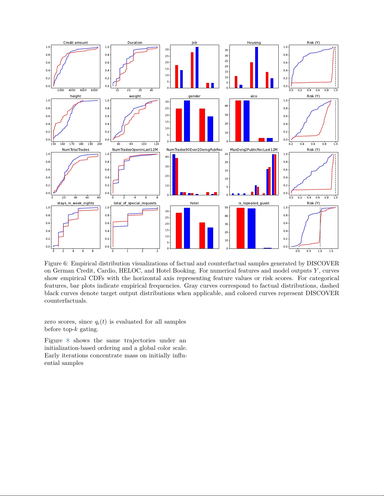
DISCO VER: A Solv er for Distributional Coun terfactual Explanations Yikai Gu 1 , Lele Cao 2 , Bo Zhao 3 , Lei Lei 4 , Lei Y ou 1 1 T echnical Univ ersity of Denmark, 2 Sc holar7, 3 Aalto Univ ersit y, 4 Xi’an Jiaotong Univ ersit y Coun terfactual explanations (CE) explain mo del decisions b y iden tifying input modiﬁcations that lead to diﬀeren t predictions. Most existing methods op erate at the instance lev el. Distributional Coun terfactual Explanations (DCE) extend this setting by optimizing an optimal transp ort objective that balances proximit y to a factual input distribution and alignmen t to a target output distribution, with statistical certiﬁcation via c hance constrained b ounds. Ho w ev er, DCE relies on gradien t based optimization, while many real-w orld tabular pip elines are dominated by non-diﬀeren tiable mo dels. W e propose DISCO VER, a mo del-agnostic solver for distributional counterfactual explanations. DISCO VER preserv es the original DCE objective and certiﬁcation while replacing gradien t descent with a sparse propose-and-select searc h paradigm. It exploits a sample-wise decomp osition of the transp ort ob jectiv e to compute p er-ro w impact scores and enforce a top- k in terv en tion budget, fo cusing edits on the most inﬂuen tial samples. T o guide candidate generation without predictor gradients, DISCO VER in troduces an OT-guided cone sampling primitive driven b y input-side transp ort geometry . Exp erimen ts on multiple tabular datasets demonstrate strong joint alignmen t of input and output distributions, extending distributional coun terfactual reasoning to modern black b o x learning pipelines. A co de rep ository is a v ailable at https://github.com/understanding- ml/DCE . Corresp ondence: leiyo@dtu.dk Date: F ebruary 2026 1 Intro duction 1.1 Background and Motivations Coun terfactual explanations (CE) are widely used in explainable artiﬁcial intelligence (XAI) to pro vide actionable insights for automated decision systems Dwiv edi et al. ( 2023 ); V erma et al. ( 2024 ). They de- scrib e minimal and feasible changes to the input that w ould lead a mo del to pro duce a desired outcome W ach ter et al. ( 2017 ). Most CE metho ds op erate at the instance level and are designed to provide recourse for a single instance, often incorporating fea- sibilit y constraints and user-sp eciﬁc costs Ustun et al. ( 2019 ); Karimi et al. ( 2020 ) or returning multiple div erse alternativ es Mothilal et al. ( 2020 ). How ever, man y real-w orld applications require p opulation-lev el in terv en tions rather than isolated edits. F or example, p olicy makers ma y ask ho w to shift the risk distribu- tion of a subgroup, or ﬁnancial institutions ma y seek systematic recourse strategies that remain consisten t with the ov erall data manifold. Existing global or group-lev el recourse to olkits partially address this is- sue by aggregating or organizing per-instance actions Ra w al and Lakkaraju ( 2020 ); Ley et al. ( 2023 ), but their ob jectiv es remain deﬁned o v er individual edits rather than distributions, and they do not directly optimize the shap e of the mo del’s output distribution that stakeholders aim to control. These settings call for distributional counterfactual explanations, where the goal is to generate a coun terfactual distribution that b oth remains close to the factual input distribu- tion and ac hiev es a desired shift in mo del outcomes. Distributional Coun terfactual Explanations (DCE) pro vides an elegant formulation of this problem using optimal transport Y ou et al. ( 2025 ). DCE balances an input-side transp ort cost that preserves plausibil- it y with an output-side transp ort cost that enforces target predictions, together with statistical certiﬁca- tion via chance-constrained b ounds. This distribu- tional p ersp ective oﬀers a principled alternativ e to instance-lev el recourse b y explicitly reasoning ab out p opulation structure and group-lev el feasibilit y . Despite its app eal, the practical adoption of DCE solv er remains limited by its optimization machinery . This gradien t-based algorithm relies on diﬀerentia- bilit y assumptions and computation graphs, which restrict its applicability to smooth predictiv e mo dels. While gradien t-based optimization is well supported for diﬀerentiable mo dels Glorot et al. ( 2011 ); Baydin 1 et al. ( 2018 ), practical tabular systems are often non- diﬀeren tiable or black-box systems, including tree en- sem bles, rule-based prepro cessing, and mixed discrete- con tin uous feature constrain ts Breiman ( 2001 ); F ried- man ( 2001 ); Sh wartz-Ziv and Armon ( 2022 ); Erick- son et al. ( 2025 ). In such settings, gradient-driv en distributional optimization b ecomes unreliable or in- feasible. More importantly , simply replacing gradients with random sampling is not suﬃcient. Distributional coun terfactual generation is a highly non-conv ex prob- lem o v er mixed-t ype spaces, where naive deriv ativ e- free search can be prohibitiv ely ineﬃcient and unsta- ble at the p opulation scale. This motiv ates the need for a solver that is model-agnostic while still exploit- ing the structure of optimal transp ort ob jectives. 1.2 Main Contributions In this work, we prop ose DISCO VER , a model- agnostic solver for distributional coun terfactual ex- planations that preserves the certiﬁed DCE ob jectiv e while rethinking the optimization paradigm. Our k ey insigh t is that optimal transp ort based distributional ob jectiv es admit a practical sample-level structure: global transp ort shifts can often b e attributed to a small subset of inﬂuential samples. A compari- son of existing counterfactual paradigms and their prop erties is summarized in T able 1 . DISCO VER op erationalizes this insight through p er- sample impact scoring and a top- k budget that local- izes and edits the most inﬂuential individuals, yield- ing a sparse and in terpretable form of distribution- lev el in terv en tion. Building on this structure, DISCOVER form ulates distributional coun terfactual generation as an itera- tiv e propose-and-select search o ver candidate coun- terfactual distributions, where multiple candidate up dates are generated and the candidate minimizing the certiﬁed DCE ob jectiv e is selected. DISCO VER further improv es blac k-b ox search by in tro ducing an input-side OT guidance primitive that exploits the geometry induced by the input- side transp ort discrepancy to steer prop osals tow ard high-plausibilit y regions without querying predictor gradien ts. • Sp arse Distributional Editing via OT De c om- p osition : W e reform ulate the distributional alignmen t problem b y unco v ering a sample- wise decomp osition of the OT ob jective. This allo ws us to in tro duce a top- k impact bud- get, lo calizing in terv en tions to the most in- ﬂuen tial samples for sparse and interpretable up dates. • Mo dular Pr op ose-and-Sele ct A r chite ctur e : W e prop ose a solv er-agnostic framework that separates candidate generation from objec- tiv e certiﬁcation. This design enables certi- ﬁed distributional counterfactual generation in non-smo oth and mixed-type spaces where traditional gradien t-based metho ds fail. • Pr e dictor-Gr adient-F r e e Ge ometric Guid- anc e : W e introduce an OT-guided cone sampling primitiv e that leverages input-side transp ort gradients. This mechanism pro- vides directed, geometry-aw are prop osals for blac k-b ox models, signiﬁcantly improvin g searc h eﬃciency ov er naiv e deriv ative-free metho ds. • Uniﬁe d Solution for Black-Box Pip elines : W e demonstrate that DISCO VER ac hiev es strong join t alignmen t of input and output distributions across diﬀeren tiable as w ell as non-diﬀeren tiable predictors, eﬀectiv ely ex- tending certiﬁed distributional reasoning to mo dern tabular pip elines. 2 Distributional Counterfactual F o rmulation and Limitations Here w e brieﬂy review the distributional counter- factual form ulation in troduced by DCE to establish notation and certiﬁcation semantics. W e then de- scrib e the combined objective used to op erationalize the chance constraints, b efore discussing why the original gradien t-based optimization becomes prob- lematic in realistic tabular pip elines. This sets the stage for the solv er redesign introduced in the next section. 2.1 Problem F ormulation Let b : R d → R b e a blac k-box model. Giv en a fac- tual input distribution x ′ with outputs y ′ = b ( x ′ ) and a target output distribution y ∗ , DCE seeks a coun- terfactual input distribution x that remains close to x ′ while aligning the model output distribution b ( x ) with y ∗ . The problem is form ulated ov er empir- ical samples and enforces robustness through chance constrain ts on b oth the input and output sides. T o measure input pro ximity , DCE emplo ys the sliced W asserstein distance S W 2 , whic h remains scalable in high dimensions, while output alignment is mea- sured using the W asserstein distance W 2 , capturing discrepancies at the distributional lev el rather than only in exp ectation Y ou et al. ( 2025 ). 2 T able 1: Comparison of counterfactual paradigms. DISCOVER keeps DCE’s distribution-level ob jectiv e and certiﬁcation, while enabling mo del-agnostic optimization with explicit top- k budgeted editing. Metho d Dist. goal Certiﬁed Model-Agnostic T op- k Instance CE No No Often Y es No Group/Global CE P artial No No No DCE Y ou et al. ( 2025 ) Y es Y es No No DISCO VER (ours) Y es Y es Y es Y es [DCE Problem] max x , P P (1) s.t. P ≤ P  S W 2 ( x , x ′ ) < U x  (2) P ≤ P  W 2  b ( x ) , y ∗  < U y  (3) P ≥ 1 − α 2 . (4) Constrain t equation 2 enforces proximit y b etw een the candidate and factual input distributions, while equation 3 imp oses the analogous requirement on the mo del outputs relative to y ∗ . The conﬁdence lev el α in equation 4 guaran tees join t satisfaction of b oth constraints with probabilit y at least 1 − α/ 2 . This c hance-constrained optimal-transport formula- tion provides interpretable, distribution-lev el align- men t while remaining scalable to high-dimensional inputs via slicing. 2.2 Distributional Counterfactual Objective Building on the formulation abov e, let Q x and Q y denote the input-side and output-side transp ort costs induced by sliced W asserstein and W asserstein dis- tances, resp ectiv ely . T o op erationalize the chance- constrained problem, DCE combines these t wo costs through an objective with a trade-oﬀ parameter η ∈ [0 , 1] , Q ( x, µ, ν , η ) ≜ (1 − η ) Q x ( x, µ ) + η Q y ( x, ν ) , (5) where µ and ν denote the corresp onding optimal transp ort plans. F or suitable choices of η , minimizing Q yields candidate solutions that satisfy the empirical c hance constrain ts in equation 2 –equation 4 with high probabilit y , highlighting the role of balancing input pro ximit y and output alignmen t. 2.3 Limitations of Gradient-Based Optimization T abular prediction tasks often rely on non- diﬀeren tiable or only piecewise smo oth mo dels Sh w artz-Ziv and Armon ( 2022 ); Erickson et al. ( 2025 ). T ree- and rule-based metho ds remain strong baselines in this setting, particularly for datasets with mixed feature t yp es, missing v alues, and structured con- strain ts Breiman ( 2001 ); F riedman ( 2001 ). Moreov er, real-w orld tabular pip elines frequen tly include pre- pro cessing steps such as discretization, thresholding, and rule-based logic, whic h can render an otherwise diﬀeren tiable mo del non-diﬀerentiable as a whole. As a result, many deploy ed tabular systems do not pro vide reliable input gradien ts. Ho w ev er, the limitations of gradient-based solv ers in distributional coun terfactual generation extend be- y ond the mere absence of gradients. The original DCE solver p erforms joint up dates of an empirical coun terfactual distribution through smo oth descen t steps, implicitly assuming that the optimization land- scap e is well behav ed under global, population-wide p erturbations. In realistic tabular settings, the dis- tributional ob jective is highly non-conv ex and de- ﬁned ov er mixed con tin uous and categorical domains, where gradients can b e unstable, noisy , or misleading ev en when diﬀeren tiabilit y holds. More fundamen tally , optimal-transp ort–based distri- butional objectives exhibit an inheren t sample-wise coupling structure: p opulation lev el shifts are often driv en by a relativ ely small subset of inﬂuen tial indi- viduals rather than uniform mov ement of all samples. This suggests that practical recourse in terven tions are naturally budgeted, in the sense that only a lim- ited num b er of instances can be meaningfully edited at eac h step while the remainder of the empirical dis- tribution should remain unc hanged. Gradient-based solv ers, which treat all samples symmetrically , fail to exploit this sparsity and can therefore pro duce ineﬃcien t or diﬃcult-to-in terpret up dates. These challenges motiv ate the need for a mo del- agnostic optimization paradigm that (i) lo calizes dis- tribution editing under an explicit top- k in terv en tion budget, and (ii) enables structured search o v er coun- terfactual distributions without relying on predictiv e mo del gradients, while preserving the certiﬁed DCE ob jectiv e. 3 3 DISCO VER: OT-Structured Spa rse Distributional Sea rch DISCO VER is a solver for Distributional Counter- factual Explanations that preserv es the DCE ob jec- tiv e and certiﬁcation lay er, while introducing an OT- structured optimization paradigm for black-box and mixed-t yp e tabular pip elines. Instead of treating dis- tribution editing as a global gradien t descen t o ver all samples, DISCO VER explicitly exploits the sample- wise structure induced by optimal transp ort. It p er- forms budgeted sparse distribution editing via top- k impact selection, and optimizes the certiﬁed ob jectiv e through a propose-and-select search ov er candidate coun terfactual distributions. All candidate distribu- tions are ev aluated by the same distribution-lev el ob jectiv e Q with the same certiﬁcation mechanism as DCE. DISCOVER does not require gradien ts of the predictiv e mo del. 3.1 DISCO VER framew ork A t each iteration, DISCO VER ﬁrst ev aluates the cur- ren t distribution using the same sliced W asserstein distance on inputs and one-dimensional W asserstein distance on outputs as in DCE. These distances are computed from empirical optimal transp ort plans and certiﬁed using the same trimmed quan tile bands and upp er-conﬁdence limits. The balance parameter η is up dated using the same interv al-narrowing rule. Therefore, DISCO VER changes neither the distribu- tional ob jectiv e nor the certiﬁcation semantics. The optimization challenge in tabular settings is not only the lac k of mo del gradien ts, but also the need for budgeted interv entions at the p opulation level. DISCO VER mak es this budget explicit. It attributes the distribution-level objective to sample-wise contri- butions and edits only a limited subset of inﬂuential instances in eac h iteration. T o operationalize this idea, DISCO VER decom- p oses the distributional objective into p er-row impact scores. On the input side, DCE induces OT plans ov er one-dimensional pro jections Θ = { θ k } N k =1 ⊂ S d − 1 . Under this plan, the input-side contribution of each sample x i can b e written as q ( x ) i = 1 N N X k =1 n X j =1   θ ⊤ k x i − θ ⊤ k x ′ j   2 µ ( k ) ij , (6) whic h measures ho w strongly x i con tributes to the curren t input-side transport discrepancy . An analo- gous decomposition holds on the output side under the transp ort plan ν , yielding q ( y ) i = n X j =1   b ( x i ) − y ∗ j   2 ν ij . (7) Sparse Distributional Sear ch Input distribution Sample-wise impact scoring T op- intervention budget Used by each strategy when updating a single feature value . Pr opose candidate distributions … Select best candidate Compare global across candidate. = 2 lar ger (c) Distribution-level global selection C1 C2 C3 C4 φ Feature 1 Feature 3 Feature 2 (b) OT -guided cone sampling … Best: (a) Sample-wise OT impact Samples ranked by lar ger OT ef fect Proposal strategy (plug -in) Genetic Monte Carlo Bayesian OT -guided cone sampling Shar ed update primitive: Output distribution DCE feasibility check Input-side OT geometry (no model gradients) T op- intervention budget Sparse distribution editing Generate per -sample influence scores and sort . Figure 1: Ov erview of DISCOVER. DISCO VER pre- serv es the DCE ob jective Q and its certiﬁcation la y er. A t eac h iteration it computes p er-sample impact scores { q i } deriv ed from the curren t OT-based ob- jectiv e, and selects a top- k activ e set that deﬁnes an explicit interv en tion budget. It then generates M candidate coun terfactual distributions b y editing only the selected samples using a shared OT-guided cone sampling primitiv e. Among the M candidates, DISCO VER selects the one with the smallest certi- ﬁed ob jective v alue Q and rep eats until the iteration budget is exhausted. Com bining both terms, the o verall p er-row impact score is deﬁned as q i = (1 − η ) q ( x ) i + η q ( y ) i . (8) Prop osition 3.1 (Ro w-wise decomp osition of the cer- tiﬁed objective) . F or ﬁxe d OT plans µ = { µ ( k ) } N k =1 and ν , the c ertiﬁe d obje ctive admits an exact r ow- wise de c omp osition Q ( x, µ, ν , η ) = P n i =1 q i , wher e q ( x ) i , q ( y ) i , and q i ar e deﬁne d ab ove. In p articular, Q x ( x, µ ) = P n i =1 q ( x ) i and Q y ( x, ν ) = P n i =1 q ( y ) i . Pro of is pro vided in App endix C . The combined score q i directly measures how strongly sample x i con tributes to the curren t certiﬁed objec- tiv e. DISCOVER uses q i to deﬁne a top- k editable set I at eac h iteration. Only rows in I ma y c hange, 4 Algorithm 1 DISCO VER: Budgeted Prop ose-and- Select Distributional Solv er Require: F actual sample X ′ , predictor b ( · ) , target outputs Y ∗ , b ounds ( U x , U y ) , conﬁdence level α , top- k budget k , candidates p er iteration M , max iterations T Ensure: Edited sample b X or ∅ 1: Initialize X ← X ′ 2: for t = 1 to T do 3: Ev aluate Q ( X ; η ) and up date η using the same certiﬁcation and in terv al-narro wing rule as DCE 4: Compute p er-ro w impact scores { q i } n i =1 5: Select editable row set I ← indices of the top- k scores 6: Compute input-side OT guidance signal g from S W 2 ( X, X ′ ) 7: Set baseline candidate X (0) ← X (no-op up- date) 8: for m = 1 to M do 9: Optimizer (Sec. 3.2 ) prop oses X ( m ) b y edit- ing rows in I using the shared OT-guided cone sampling primitive (Sec. 3.3 ) guided by − g 10: end for 11: b X ← arg min m ∈{ 0 , 1 ,...,M } Q  X ( m ) ; η  12: X ← b X 13: end for 14: Chec k whether b X satisﬁes the same DCE certiﬁ- cation criteria 15: if certiﬁcation holds then 16: return b X 17: else 18: return ∅ 19: end if and all other rows remain ﬁxed. This top- k gate implemen ts an explicit interv ention budget. It re- duces the eﬀectiv e searc h space, impro ves stability , and yields sparse and in terpretable p opulation-level edits, while k eeping the ob jective unchanged. Giv en the editable set I , DISCO VER performs a distribution-lev el propose-and-select search. It gen- erates M candidate coun terfactual distributions by editing only ro ws in I with a shared proposal prim- itiv e. Eac h candidate is ev aluated by the same cer- tiﬁed ob jective Q ( · ; η ) , and the b est candidate is selected as the next iterate. W e additionally include the curren t distribution as a baseline no-op candidate (Algorithm 1 ), which guarantees that the certiﬁed ob jectiv e do es not increase within each iteration. Prop osition 3.2 (Monotonicity of the prop ose-and-s- elect step) . L et X b e the curr ent iter ate and let b X = arg min m ∈{ 0 , 1 ,...,M } Q ( X ( m ) ; η ) b e the sele cte d c andidate, wher e X (0) = X is the no-op pr op osal and η is ﬁxe d during the c andidate evaluation. Then Q ( b X ; η ) ≤ Q ( X ; η ) . Pro of is pro vided in App endix C . This explicit candidate selection is a k ey diﬀerence from single-path descen t methods and is well-suited for non-conv ex and mixed-type optimization land- scap es. T o bias prop osals tow ard low input distortion with- out querying predictive mo del gradients, DISCO VER computes an input-side OT guidance ﬁeld from S W 2 ( X, X ′ ) and uses it only in the prop osal step. The output side remains fully blac k-box because no ∇ b is required. After the iteration budget, DIS- CO VER returns the b est candidate that satisﬁes the same DCE certiﬁcation criteria. 3.2 A Modular Prop osal Mechanism fo r Distributional Sea rch DISCO VER separates the certiﬁed distributional ob- jectiv e from the mechanism that proposes candidate distributions. The mo dular optimizer is a proposal la y er. It receives the current iterate X , the editable ro w set I induced b y the top- k in terv en tion bud- get, and a small set of exploration parameters. It outputs M candidate distributions { X ( m ) } M m =1 that only edit ro ws in I and satisfy domain constraints and actionabilit y rules. All optimizers share a com- mon proposal primitiv e, OT-guided cone sampling (Sec. 3.3 ), and diﬀer only in how they com bine and apply it to generate candidates. Diﬀeren t optimizers diﬀer only in how they propose candidates. All candidates are ev aluated by the same certiﬁed ob jectiv e Q ( · ; η ) , and DISCOVER selects the b est candidate. This makes the ov erall solver strategy-agnostic while k eeping a single ob jective and a single certiﬁcation proto col. Mon te Carlo Optimizer. The Monte Carlo opti- mizer prop oses M v alidity-preserving candidate edits around the curren t iterate. The top- k gate conﬁnes c hanges to the most inﬂuential ro ws, and an input- side OT guidance ﬁeld g = ∇ X S W 2 ( X, X ′ ) biases prop osal directions. Numerical features are p erturb ed within v alid ranges, and categorical features are mod- iﬁed within admissible lev els. Among the M candi- dates, DISCO VER selects the one with the smallest certiﬁed ob jectiv e v alue. 5 Genetic Optimizer. The genetic optimizer pro- duces candidates through recombination and guided m utation on the same editable set I . Crossov er reuses partial structures from the curren t iterate, while m utations introduce lo cal v ariations in a domain– preserving manner. Both operations are biased b y the same input–side guidance ﬁeld g . Each candidate is ev aluated b y Q ( · ; η ) , and DISCO VER selects the b est candidate. 3.3 OT-Guided Cone Sampling Primitive Edits are restricted to the curren t top- k ro ws I , so that each iteration focuses on the samples under the in terv en tion budget. T o guide candidate generation without relying on mo del gradients, DISCOVER com- putes a single input-side guidance ﬁeld − g = −∇ x S W 2 ( x, x ′ ) , whic h dep ends only on the sliced W asserstein distance b et w een the current distribution and the factual ref- erence. This ﬁeld captures geometry of input-side transp ort under the curren t OT structure. It is in- dep enden t of the predictiv e mo del, and ∇ b is nev er queried. The guidance ﬁeld g is used only to bias prop osal directions. Candidate up dates are sampled within a cone of half-angle ϕ around the direction − g , tak e b ounded steps, and are pro jected bac k to the v alid domain. No gradient descent is p erformed on the full ob jectiv e Q , and ∇ b is nev er queried. The guid- ance ﬁeld is ev aluated once p er outer iteration and reused across all M candidate trials generated by the mo dular optimizer, ensuring low o verhead while main taining consisten t directional bias. Algorithm 2 OT-guided cone sampling for numeri- cal features 1: Input: row index i , current ro w x i · , ed- itable indices R , guidance g , feature ranges { [ R min p , R max p ] } p ∈R 2: Output: up dated row x i · on R 3: for p ∈ R do 4: sample direction d ip in a cone around − g (half- angle ϕ ) 5: sample a step size λ ∈ [0 , λ max ] 6: up date x ip ← Π [ R min p ,R max p ]  x ip + λ ( R max p − R min p ) d ip  7: end for 8: return up dated x i · Numerical co ordinates. F or n umerical features, DISCO VER generates prop osals using a shared OT- guided cone sampling primitive. Each editable ro w is up dated by sampling a direction that is biased to- w ard the negativ e input-side guidance ﬁeld − g , where g = ∇ X S W 2 ( X, X ′ ) depends on the transport dis- crepancy to the factual distribution. This pro vides a ligh t w eigh t geometric prior that fa vors low-distortion edits in the input space, without requiring an y gradi- en t information from the predictiv e mo del. The cone half-angle ϕ con trols the concen tration of prop osals around this OT-induced direction, inter- p olating b etw een focused transp ort-consistent mo v es and broader exploration. A b ounded step size λ ∈ [0 , λ max ] is dra wn and scaled b y the feature range ( R max p − R min p ) to normalize up dates across heterogeneous units. Each proposed update is ﬁnally pro jected onto the v alid in terv al [ R min p , R max p ] , en- suring feasibility by construction. This pro cedure yields n umerical candidate distributions that pre- serv e input-side plausibilit y while enabling eﬀectiv e distribution-lev el searc h under the top- k in terv en tion budget. Algorithm 3 OT-guided cone sampling for categori- cal features 1: Input: row index i , curren t row x i · , editable indices C , guidance g , temp erature τ 2: Output: up dated row x i · on C 3: for p ∈ C do 4: represen t category x ip as a one-hot vector o ip ∈ { 0 , 1 } |V p | 5: em b ed z ip ← E p [ x ip ] where E p ∈ R |V p |× r is a ﬁxed em bedding table (initialized once and k ept constan t) 6: tak e a cone-biased em b edding step: ˜ z ip ← z ip + ∆ , where ∆ ∈ R r is sampled in a cone around − g (half-angle ϕ ) 7: include the no-op option v = x ip in the admis- sible set under actionabilit y constrain ts 8: deco de by sampling a category with Pr ( v ) ∝ exp  −∥ E p [ v ] − ˜ z ip ∥ 2 /τ  under actionability constrain ts 9: end for 10: return up dated x i · Categorical co ordinates. F or categorical features, DISCO VER performs prop osals in a n umerical em- b edding space where directions are meaningful. F or eac h categorical feature p , w e construct a ﬁxed em- b edding table E p ∈ R |V p |× r once b efore optimization and k eep it constan t throughout. In our implementa- tion, E p is randomly initialized with a ﬁxed random state for reproducibility , and r is c hosen b y a deter- ministic rule based on the category cardinality |V p | unless speciﬁed. A cone-biased step guided b y − g is then applied in the em bedding space. T o deco de 6 0 5 OT Distance ARES 0 5 OT Distance GLobe 0 5 OT Distance DiCE 0 5 OT Distance DCE 0 5 10 15 20 25 30 35 40 Sample Index 0 5 OT Distance DISCO VER Samplewise OT (40 samples) Figure 2: Per-sample input-side OT distances on COMP AS with an MLP . Distances are sorted in de- scending order within each metho d, highlighting the top-10 largest v alues. All metho ds share the same y-axis scale for fair comparison. bac k to a discrete category , we compute distances b et w een the updated em b edding and all category em- b eddings and sample with a temperature-controlled rule. Sp eciﬁcally , the probabilit y of category v is pro- p ortional to exp ( −∥ E p [ v ] − ˜ z ∥ 2 /τ ) , where E p [ v ] ∈ R r denotes the embedding vector of category v . The tem- p erature τ con trols the exploration and exploitation trade-oﬀ. Finally , deco ding is restricted to admissible categories under predeﬁned domain and actionabilit y constrain ts. 4 Exp erimental Setup and Results 4.1 Exp erimental Setup W e ev aluate DISCO VER mainly on ﬁve tabular datasets: HELOC FICO ( 2018 ), COMP AS Larson et al. ( 2016 ), Hotel Booking Antonio et al. ( 2019 ), German Credit Hofmann ( 1994 ), and Cardiov ascu- lar Disease Halder ( 2020 ). Quantitativ e compar- isons are p erformed on HELOC, COMP AS and Ger- man Credit, where DISCOVER is compared with existing CE metho ds, including DCE Y ou et al. ( 2025 ), DiCE Mothilal et al. ( 2020 ), AReS Raw al and Lakkara ju ( 2020 ), and GLOBE Ley et al. ( 2023 ). DiCE generates counterfactuals indep endently for individual instances, whereas AReS and GLOBE 0.0 0.2 0.4 0.6 0.8 1.0 Risk Probability (Y) 0.0 0.2 0.4 0.6 0.8 1.0 Cumulative Probability (Quantile) Empirical CDF Comparison (Y) DCE F actual AR eS GL OBE DiCE DISCO VER T ar get Figure 3: Empirical CDF s of mo del output distri- butions on COMP AS with an MLP . Sho wn are the factual outputs, the target distribution, and coun ter- factual outputs pro duced b y diﬀerent metho ds. op erate at the group lev el by aggregating recourse patterns across samples. DCE is included as a gradien t-based baseline in settings where diﬀeren- tiabilit y is a v ailable, enabling a direct comparison b e- t w een gradient-bas ed optimization and the prop osed mo del-agnostic solver under the s ame distributional ob jectiv es. The main ev aluation targets the distributional align- men t ob jective inherited from DCE. W e primarily rep ort OT ( x ) and OT ( y ) , which quantify input-side plausibilit y preserv ation and output-side target at- tainmen t, resp ectively . W e also rep ort MMD and AReS Cost to match prior ev aluation proto cols. Ab- lation test the necessity of DISCO VER’s solv er com- p onen ts: (i) sample-wise OT impact scoring and the top- k in terv en tion budget, (ii) propose-and-select candidate searc h ov er multiple prop osals p er itera- tion, and (iii) OT-guided cone sampling as a shared prop osal primitiv e. Extended results and additional settings are rep orted in the App endix D and E . 4.2 Main Results Figures 2 and 3 pro vide a qualitative comparison of input distortion and output shift across methods. Conserv ative metho ds can preserv e the input distri- bution while failing to induce a meaningful output shift. AReS pro duces uniformly small p er-sample input-side transport distances, but its output CDF remains close to the factual distribution, leading to 7 T able 2: Comparison of DISCOVER with CE baselines on tabular datasets. W e rep ort Diﬀ. and Non-diﬀ. mo dels. OT ( x ) / OT ( y ) are input/output W asserstein distances and our primary distributional criteria (lo w er is b etter). AReS Cost is rep orted for reference only (not optimized by DISCO VER). DCE is included only in Diﬀ. settings. Results are mean ± 80% CI ov er SVM, MLP , RF, X GBoost, and Ligh tGBM. Gray en tries are excluded; b old denotes b est among remaining metho ds. Dataset Method OT( x ) OT( y ) MMD AReS Cost COMP AS (Diﬀ.) AReS 0 . 0222 ± 0 . 0566 0 . 5389 ± 0 . 0425 0 . 0261 ± 0 . 0713 2 . 0764 ± 2 . 0380 GLOBE 20 . 5166 ± 53 . 6786 0 . 0088 ± 0 . 0271 0 . 2422 ± 0 . 0499 1 . 0703 ± 1 . 8080 DiCE 0 . 1124 ± 0 . 0863 0 . 2273 ± 0 . 0505 0.0553 ± 0.0129 3.9354 ± 0.0057 DCE 0 . 0930 ± 0 . 0220 0 . 1576 ± 0 . 0300 0 . 0894 ± 0 . 0211 4 . 0677 ± 1 . 1666 DISCOVER 0.0681 ± 0.0252 0.1474 ± 0.0576 0 . 0679 ± 0 . 0203 4 . 0370 ± 0 . 6362 COMP AS (Non-diﬀ.) AReS 0 . 0174 ± 0 . 0195 0 . 4990 ± 0 . 1350 0 . 0281 ± 0 . 0349 0 . 9278 ± 0 . 8920 GLOBE 0 . 3537 ± 0 . 0275 0 . 2480 ± 0 . 0166 0 . 2031 ± 0 . 0258 1.4250 ± 0.8522 DiCE 0 . 0673 ± 0 . 0045 0 . 2376 ± 0 . 0329 0 . 0867 ± 0 . 0064 2 . 2813 ± 0 . 4523 DCE – – – – DISCOVER 0.0586 ± 0.0021 0.1412 ± 0.0473 0.0838 ± 0.0103 2 . 9224 ± 0 . 0981 HELOC (Diﬀ.) AReS 0 . 0005 ± 0 . 0005 0 . 2956 ± 0 . 0045 0 . 0003 ± 0 . 0003 1 . 7751 ± 4 . 8569 GLOBE 1 . 5997 ± 0 . 2901 0 . 1166 ± 0 . 0302 0 . 0060 ± 0 . 0003 2 . 5810 ± 0 . 0673 DiCE 0 . 0218 ± 0 . 0180 0 . 1641 ± 0 . 0606 0 . 0054 ± 0 . 0003 5.5336 ± 5.1293 DCE 0 . 1196 ± 0 . 1408 0.1381 ± 0.1074 0 . 0152 ± 0 . 0069 6 . 3231 ± 0 . 2319 DISCOVER 0.0139 ± 0.0112 0 . 1897 ± 0 . 0245 0.0033 ± 0.0021 9 . 4846 ± 0 . 1944 HELOC (Non-diﬀ.) AReS 0 . 0008 ± 0 . 0002 0 . 5184 ± 0 . 1966 0 . 0007 ± 0 . 0002 0 . 0738 ± 0 . 0043 GLOBE 6 . 6634 ± 5 . 5036 0 . 1138 ± 0 . 0823 0 . 0602 ± 0 . 0507 2 . 5813 ± 0 . 1247 DiCE 0 . 0704 ± 0 . 0412 0 . 2315 ± 0 . 0423 0 . 0455 ± 0 . 0371 3.9318 ± 2.0387 DCE – – – – DISCOVER 0.0514 ± 0.0479 0.1595 ± 0.0353 0.0320 ± 0.0264 3 . 9616 ± 1 . 9334 German Credit (Diﬀ.) AReS 0 . 0182 ± 0 . 0548 0 . 7827 ± 1 . 2471 0 . 0306 ± 0 . 0891 0 . 8536 ± 0 . 4507 GLOBE 230 . 8465 ± 468 . 6101 0 . 0082 ± 0 . 0252 0 . 2499 ± 0 . 5466 0 . 2164 ± 0 . 0719 DiCE 0 . 0552 ± 0 . 1437 0 . 1101 ± 0 . 2879 0 . 1196 ± 0 . 2364 4 . 5631 ± 10 . 1682 DCE 0.0213 ± 0.0234 0 . 5214 ± 0 . 4393 0.0324 ± 0.0131 5 . 8666 ± 17 . 4976 DISCOVER 0 . 0465 ± 0 . 1253 0.1025 ± 0.0922 0 . 0969 ± 0 . 1988 2.8578 ± 4.1513 German Credit (Non-diﬀ.) AReS 0 . 0029 ± 0 . 0030 0 . 6675 ± 0 . 2290 0 . 0079 ± 0 . 0068 1 . 1267 ± 1 . 1450 GLOBE 0 . 0300 ± 0 . 0046 0 . 3609 ± 0 . 0041 0 . 0519 ± 0 . 0135 0.9147 ± 0.1440 DiCE 0 . 0124 ± 0 . 0083 0 . 3636 ± 0 . 1834 0.0468 ± 0.0304 5 . 0579 ± 0 . 7173 DCE – – – – DISCOVER 0.0117 ± 0.0070 0.2285 ± 0.0528 0 . 0470 ± 0 . 0323 6 . 9458 ± 1 . 7376 large OT( y ) . In contrast, aggressive group-lev el translations can matc h the target outputs while severely distorting inputs. GLOBE aligns the output distribution closely to the target, but does so with substan tially larger p er-sample OT( x ) , indicating global distortion. DISCO VER achiev es a sparse and co ordinated in- terv en tion pattern. It concen trates edits on a small subset of inﬂuential samples, yielding a controlled OT ( x ) proﬁle while producing an output CDF that closely tracks the target. This supp orts the moti- v ation b ehind budgeted sparse distribution editing: eﬀectiv e distributional explanations require selective, co ordinated edits rather than uniformly small or uni- formly large c hanges. W e rep ort the main quan titative comparison in T a- ble 2 . Results are av eraged ov er ﬁve predictiv e mo dels (SVM, MLP , Random F orest, XGBoost, and Light- GBM) and are rep orted separately for diﬀerentiable and non-diﬀeren tiable settings. W e fo cuse primarily on OT ( x ) and OT ( y ) , which re- sp ectiv ely measure the W asserstein distance betw een the factual and counterfactual input and output dis- tributions. These metrics directly reﬂect the quality of distributional counterfactual explanations, as they assess whether coun terfactual edits simultaneously preserv e the structure of the input distribution while steering mo del predictions tow ard the desired target distribution. A cross datasets, DISCO VER attains the b est or second-b est OT ( x ) in most settings and ac hieves the lo w est OT( y ) in all non diﬀerentiable settings. In contrast, sev eral baseline methods exhibit im- balanced b ehavior betw een OT ( x ) and OT ( y ) . F or instance, AReS frequently attains extremely small OT ( x ) and MMD v alues, suggesting minimal pertur- bations to the input distribution. How ev er, this be- ha vior is accompanied by substan tially larger OT ( y ) v alues in nearly all cases, sho wing that the output distribution remains far from the target. This re- ﬂects the rule-based nature of AReS, which prioritizes 8 0 50 100 0.0 0.2 0.4 0.6 OT V alue Ger man Cr edit (cone) OT(x) OT(y) Q 0 50 100 0.0 0.1 0.2 0.3 0.4 Heloc_LGBM (h=2) 0 50 100 0.0 0.1 0.2 0.3 0.4 Compas_SVM (k=3) 0 50 100 0.0 0.1 0.2 0.3 0.4 Car dio_RF (Monte Carlo) 0 50 0.0 0.2 0.4 0.6 0.8 Q vs Iteration Infeasible F easible 0 50 100 0.0 0.2 0.4 0.6 OT V alue Ger man Cr edit (original) 0 50 100 0.0 0.1 0.2 0.3 0.4 Heloc_LGBM(h=8) 0 50 100 0.0 0.1 0.2 0.3 0.4 Compas_SVM (k=10) 0 50 100 0.0 0.1 0.2 0.3 0.4 Car dio_RF (Genetic) 0 50 100 0.0 0.2 0.4 0.6 0.8 OT(x), OT(y) O T ( x ) O T ( y ) Figure 4: Optimization dynamics of DISCO VER across datasets and mo del arc hitectures. Each subplot sho ws OT ( x ) , OT ( y ) , and the ob jectiv e Q o v er iterations. OT ( x ) (blue) measures input-side W asserstein distance, and OT ( y ) (orange) measures output-side distance to the target. Solid lines denote the mean ov er ﬁve random seeds, with shaded regions indicating standard deviation. Results sho w stable and consistent conv ergence across datasets, mo dels, and solver settings. conserv ative feature edits and feasibilit y constraints, often at the expense of ac hieving meaningful distri- butional shifts in mo del predictions. This leads to coun terfactual distributions that remain close to the factual outputs under the OT criterion. Similarly , DiCE, as an instance-based method, strug- gles to co ordinate counterfactual edits across sam- ples. While it may ac hieve reasonable OT( x ) v alues in some settings, its OT ( y ) v alues are consistently higher than those of DISCOVER, indicating limited abilit y to align output distributions at the group level. This is consistent with the limitation of instance-wise generation when the ev aluation target is deﬁned ov er distributions. GLOBE exhibits high v ariance and occasionally ex- tremely large OT ( x ) v alues (e.g., German Credit), while achieving very small OT ( y ) . This indicates that GLOBE can reach output alignmen t by applying large, near-uniform translations across man y samples, whic h mov es the empirical input distribution far from the factual manifold. Because OT ( x ) is a distribution- lev el transp ort distance, a small num b er of failed or o v erly aggressive runs can dominate the mean and inﬂate the conﬁdence in terv al. W e therefore in terpret these results as evidence that translation-based group recourse can b e unstable under mixed constraints, and we complement mean statistics with p er-sample proﬁles in Figure 2 . The original DCE metho d is included as a baseline in diﬀeren tiable settings. Although DCE and DIS- CO VER optimize the same certiﬁed distributional ob- jectiv e, DISCO VER remains competitive with DCE and can sometimes ac hiev e lo w er OT ( x ) / OT ( y ) un- der the same ev aluation budget. W e attribute this b eha vior to the solver paradigm rather than a change of ob jectiv e. DCE follows a single-path gradient de- scen t that up dates all samples sim ultaneously , which can b e sensitive to non-con vexit y , slicing approxima- tions, and mixed-t ype constraints. In contrast, DIS- CO VER p erforms budgeted sparse edits and applies a prop ose-and-select searc h o v er m ultiple candidate distributions, pro viding a more robust up date mech- anism under sto c hastic and discrete prop osal dynam- ics. Consistent with this explanation, Figure 4 sho ws that OT-guided prop osals stabilize optimization tra- jectories, while ov erly aggressive population up dates (larger k ) lead to unstable behavior. Additional abla- tions on k ey solv er components are reported in the App endix D . 4.3 Ablation Study W e ablate solv er components (Figure 4 ) and editable feature subsets (T able 3 ), and sw eep h and k to study stabilit y–eﬃciency trade-oﬀs under a ﬁxed ev aluation budget. T able 3 shows that allowing b oth numerical and cat- egorical edits generally yields the low est OT ( x ) . Re- 9 T able 3: Ablation of editable feature subsets. Results are av eraged o v er mo dels (treated as indep endent runs) and rep orted as mean ± 95% conﬁdence interv al. F or each dataset, the b est (low est) v alue for eac h metric is highligh ted in b old. Dataset Method OT( x ) OT( y ) MMD AReS Cost COMP AS DISCOVER 0.112800 ± 0.038690 0.028067 ± 0.007056 0.046067 ± 0.012027 8.643200 ± 0.813492 Categorical only 0.142267 ± 0.041301 0.029733 ± 0.006039 0.049400 ± 0.010146 8.800867 ± 0.864495 numerical only 0.118333 ± 0.039038 0.024933 ± 0.006147 0.046867 ± 0.010116 8.742867 ± 0.669316 No editing 0.140867 ± 0.040595 0.028533 ± 0.005470 0.049667 ± 0.008073 9.123267 ± 0.613175 Cardio DISCOVER 0.052900 ± 0.008728 0.019350 ± 0.002854 0.022300 ± 0.001457 7.216050 ± 0.461864 Categorical only 0.076800 ± 0.018989 0.014000 ± 0.003957 0.026750 ± 0.001730 7.447850 ± 0.497926 numerical only 0.065000 ± 0.008903 0.020600 ± 0.003084 0.027950 ± 0.001596 8.578950 ± 0.454685 No editing 0.090850 ± 0.018019 0.015500 ± 0.003870 0.032600 ± 0.002106 8.797000 ± 0.543489 HELOC DISCOVER 0.096000 ± 0.015814 0.059650 ± 0.017533 0.027950 ± 0.001819 7.748600 ± 0.622564 Categorical only 0.149000 ± 0.022498 0.059950 ± 0.018815 0.029500 ± 0.001863 8.817000 ± 0.804573 numerical only 0.109700 ± 0.018299 0.056550 ± 0.017828 0.029150 ± 0.001651 8.196950 ± 1.058611 No editing 0.160500 ± 0.025151 0.057250 ± 0.018835 0.029500 ± 0.001639 9.648950 ± 0.817946 German Credit DISCOVER 0.112600 ± 0.015718 0.043000 ± 0.024616 0.033900 ± 0.002087 7.534250 ± 0.273088 Categorical only 0.189250 ± 0.033634 0.048850 ± 0.026457 0.035700 ± 0.001692 7.282100 ± 0.237567 numerical only 0.103700 ± 0.015955 0.040800 ± 0.024742 0.035300 ± 0.001860 8.544250 ± 0.341697 No editing 0.163100 ± 0.024923 0.041900 ± 0.025018 0.037700 ± 0.001758 8.369600 ± 0.267596 Hotel Bo oking DISCOVER 0.108120 ± 0.022602 0.025680 ± 0.009189 0.025880 ± 0.001285 16.480120 ± 2.742385 Categorical only 0.193640 ± 0.073230 0.034840 ± 0.016852 0.025960 ± 0.001302 18.282440 ± 3.372114 numerical only 0.124960 ± 0.027583 0.019200 ± 0.007702 0.027040 ± 0.001324 15.646160 ± 2.546458 No editing 0.177160 ± 0.050751 0.029120 ± 0.015467 0.027000 ± 0.001294 18.604800 ± 3.164555 stricting edits to a single t yp e often increases OT ( x ) , indicating reduced ﬂexibility for transport-consistent lo w-distortion up dates. F or OT ( y ) , n umerical-only editing is often comp eti- tiv e (e.g., COMP AS, HELOC, German Credit, and Hotel Bo oking), while categorical edits matter on datasets where discrete switches are needed (e.g., Car- dio). Overall, enabling both t yp es provides the most reliable balance betw een OT ( x ) and OT ( y ) . This is consisten t with the ob jectiv e structure: numerical ed- its follo w the con tin uous geometry of S W 2 , whereas categorical edits introduce discrete mo v es that can b e harder to optimize but sometimes necessary . Numerical up dates align well with the contin uous geometry induced by S W 2 , while categorical updates in tro duce discrete jumps that can b e harder to op- timize but may b e necessary to achiev e target align- men t under constrain ts. Figure 4 summarizes optimization tra jectories of OT ( x ) , OT ( y ) , and Q across datasets, models, and solv er settings. Column 1 compares German Credit under tw o set- tings: with OT-guided cone sampling (top) and with- out it (b ottom). When cone guidance is enabled, all three quan tities decrease smo othly and remain stable. Without guidance, OT ( x ) shows large ﬂuctuations, whic h propagate to the ob jectiv e Q . As a result, b oth the ﬁnal OT ( x ) and OT ( y ) v alues and the ob jective are worse than in the guided case, highlighting the stabilizing role of input-side geometric guidance. The second column analyzes the eﬀect of h , the n um- b er of features up dated p er selected sample, on HE- LOC with Ligh tGBM. Increasing h from 2 to 8 leads to faster con v ergence. The v ariance of Q and OT ( y ) is substantially larger for h = 2 , while h = 8 yields smo other trajectories. Larger h accelerates the de- crease of Q and OT ( y ) , at the cost of a modest in- crease in OT( x ) v ariance. The third column studies the impact of k , the n um b er of samples up dated p er iteration, on COMP AS with an SVM. With k = 3 , OT ( x ) , OT ( y ) , and Q con v erge smo othly and remain stable. In contrast, k = 10 leads to large ﬂuctuations and wide v ariance bands, and the ﬁnal solution is inferior across all metrics. This supp orts the top- k design: sparse interv en tions stabilize the OT objective, while large- k up dates amplify coupling noise. The fourth column compares Monte Carlo and Ge- netic optimizers on Cardio with a Random F orest. Both optimizers reac h similar mean tra jectories and ﬁnal v alues of Q . How ev er, Monte Carlo exhibits noticeably larger v ariance, reﬂecting higher stochas- ticit y across runs. The last column visualizes feasibility during optimiza- tion. The top panel plots Q , where purple indicates infeasible iterates and y ello w indicates feasible ones. After a ﬁnite n um b er of iterations, marked by the ver- tical dashed line, the optimization enters the feasible region. The b ottom panel sho ws that this transition coincides with a balance b etw een OT ( x ) and OT ( y ) , conﬁrming that feasibility is achiev ed when input 10 pro ximit y and output alignment are join tly satisﬁed. 5 Conclusion In this paper, we in tro duced DISCOVER, a mo del- agnostic solver for distributional counterfactual expla- nations that preserv es the certiﬁed optimal-transp ort ob jectiv e of DCE. DISCO VER identiﬁes inﬂuential samples through a sample-wise OT decomp osition and applies a top- k in terv en tion budget to lo calize distributional edits. A cross m ultiple tabular datasets and predictors, DISCOVER achiev es strong align- men t betw een input and output distributions. Cru- cially , these impro v emen ts are obtained without re- lying on predictiv e model gradien ts. As a modular and architecture-agnostic approach, DISCOVER inte- grates naturally with blac k-b o x tabular pipelines and broadens the applicabilit y of certiﬁed distributional explanations. References Nuno Antonio, Ana de Almeida, and Luis Nunes. Hotel b ooking demand datasets. Data in brief , 22:41–49, 2019. A tilim Gunes Ba ydin, Barak A Pearlm utter, Alexey An- drey evich Radul, and Jeﬀrey Mark Siskind. A utomatic diﬀeren tiation in mac hine learning: a surv ey . Journal of machine le arning r ese ar ch , 18(153):1–43, 2018. Leo Breiman. Random forests. Machine le arning , 45(1): 5–32, 2001. Susanne Dandl, Kristin Blesch, Timo F reiesleb en, Gunnar König, Jan Kapar, Bernd Bisc hl, and Marvin N W right. Coun tarfactuals–generating plausible model-agnostic coun terfactual explanations with adv ersarial random forests. In W orld Confer enc e on Explainable A rtiﬁcial Intel ligenc e , pages 85–107, 2024. Sopam Dasgupta, Sadaf Halim, Joaquín Arias, Elmer Salazar, and Gopal Gupta. Mc3g: Mo del agnostic causally constrained coun terfactual generation. arXiv pr eprint arXiv:2508.17221 , 2025. R udresh Dwivedi, Dev am Dav e, Het Naik, Smiti Singhal, Rana Omer, Pank esh P atel, Bin Qian, Zhenyu W en, T ejal Shah, Graham Morgan, et al. Explainable ai (xai): Core ideas, techniques, and solutions. A CM c omputing surveys , 55(9):1–33, 2023. Nic k Eric kson, Lennart Puruc ker, Andrej T sc halzev, Da vid Holzmüller, Prateek Mutalik Desai, David Sali- nas, and F rank Hutter. T abarena: A living benchmark for machine learning on tabular data. arXiv pr eprint arXiv:2506.16791 , 2025. FICO. Fico explainable machine learning challenge, 2018. Jerome H F riedman. Greedy function appro ximation: a gradien t b o osting machine. A nnals of statistics , 29(5): 1189–1232, 2001. Xa vier Glorot, An toine Bordes, and Y oshua Bengio. Deep sparse rectiﬁer neural netw orks. In 14th International Confer enc e on A rtiﬁcial Intel ligenc e and Statistics , v ol- ume 15, pages 315–323, 2011. Riccardo Guidotti. Coun terfactual explanations and how to ﬁnd them: Literature review and benchmarking. Data Mining and K now le dge Discovery , pages 1–55, 2022. R. K. Halder. Cardiov ascular disease dataset, 2020. Hans Hofmann. Statlog (german credit data), 1994. UCI Mac hine Learning Repository . Amir-Hossein Karimi, Gilles Barthe, Borja Balle, and Isab el V alera. Model-agnostic counterfactual expla- nations for consequential decisions. In International c onfer enc e on artiﬁcial intel ligenc e and statistics , pages 895–905, 2020. Jeﬀ Larson, Lauren Kirchner, Sury a Mattu, and Julia Angwin. How we analyzed the compas recidivism algo- rithm, 2016. Dan Ley , Saumitra Mishra, and Daniele Magazzeni. Glob e-ce: A translation based approach for global coun- terfactual explanations. In International c onfer enc e on machine le arning , pages 19315–19342, 2023. Ramara vind K Mothilal, Amit Sharma, and Chenhao T an. Explaining mac hine learning classiﬁers through div erse coun terfactual explanations. In Pr o c e e dings of the 2020 confer enc e on fairness, ac c ountability, and tr ansp ar ency , pages 607–617, 2020. Gabriel Peyré, Marco Cuturi, et al. Computational op- timal transp ort: With applications to data science. F oundations and T r ends ® in Machine L e arning , 11 (5-6):355–607, 2019. Gregory Plum b, Jonathan T erhorst, Sriram Sankarara- man, and Ameet T alwalkar. Explaining groups of p oin ts in low-dimensional represen tations. In Interna- tional Confer ence on Machine L e arning , pages 7762– 7771, 2020. Rafael Po yiadzi, Kacper Sok ol, Raul San tos-Ro driguez, Tijl De Bie, and Peter Flach. F ace: feasible and action- able counterfactual explanations. In Pro ce e dings of the AAAI/A CM Confer enc e on AI, Ethics, and So ciety , pages 344–350, 2020. Kaiv alya Raw al and Himabindu Lakkara ju. Beyond in- dividualized recourse: In terpretable and interactiv e summaries of actionable recourses. A dvanc es in Neur al Information Pr o c essing Systems , 33:12187–12198, 2020. Rob ert-Florian Samoilescu, Arnaud V an Loov eren, and Janis Klaise. Mo del-agnostic and scalable coun terfac- tual explanations via re inforcement learning. arXiv pr eprint arXiv:2106.02597 , 2021. Ra vid Shw artz-Ziv and Amitai Armon. T abular data: 11 Deep learning is not all y ou need. Information F usion , 81:84–90, 2022. Berk Ustun, Alexander Spangher, and Y ang Liu. Action- able recourse in linear classiﬁcation. In Pr o c e e dings of the c onfer enc e on fairness, acc ountability, and tr ans- p ar ency , pages 10–19, 2019. Sahil V erma, V arich Boonsanong, Minh Hoang, Keegan Hines, John Dic k erson, and Chirag Shah. Counterfac- tual explanations and algorithmic recourses for machine learning: A review. A CM Computing Surveys , 56(12): 1–42, 2024. Sandra W ach ter, Brent Mittelstadt, and Chris R ussell. Coun terfactual explanations without opening the blac k b o x: A utomated decisions and the gdpr. Harv. JL & T ech. , 31:841, 2017. Geemi P W ella w atte, Aditi Seshadri, and Andrew D White. Model agnostic generation of counterfactual explanations for molecules. Chemic al scienc e , 13(13): 3697–3705, 2022. W enzhuo Y ang, Jia Li, Caiming Xiong, and Stev en CH Hoi. Mace: An eﬃcient mo del-agnostic frame- w ork for counterfactual explanation. arXiv pr eprint arXiv:2205.15540 , 2022. Lei Y ou, Lele Cao, Mattias Nilsson, Bo Zhao, and Lei Lei. Distributional counterfactual explanations with optimal transp ort. In International Confer enc e on A rtiﬁcial Intel ligenc e and Statistics , pages 1135–1143, 2025. Lei Y ou, Yijun Bian, and Lele Cao. Joint distribu- tion–informed shapley v alues for sparse coun terfac- tual explanations. In The F ourte enth International Confer enc e on L e arning R epr esentations , 2026. URL https://openreview.net/forum?id=3vIe5pNiUN . 12 A Related W o rk Coun terfactual explanations (CE) aim to provide ac- tionable insight b y identifying feasible input changes that alter a mo del prediction. W ach ter et al. W ach ter et al. ( 2017 ) form ulate CE as an optimization prob- lem that balances pro ximit y to the factual instance and alignment with a target outcome, whic h has motiv ated a broad literature Guidotti ( 2022 ). Instance-lev el coun terfactuals and recourse. Most existing methods generate counterfactuals for individual instances. They incorp orate feasibility constrain ts, immutable features, and user-deﬁned costs to ensure v alid edits P oyiadzi et al. ( 2020 ); Ustun et al. ( 2019 ); Karimi et al. ( 2020 ), and extend this setting to pro duce diverse counterfactual sets for a single instance Mothilal et al. ( 2020 ). These approac hes are eﬀectiv e for individual recourse, but their ob jectives and guarantees are deﬁned at the instance lev el. Group-lev el and global summaries. Recent w ork also considers cohort-lev el recourse and global summaries. AReS Raw al and Lakkara ju ( 2020 ) summarizes actionable recourse patterns for sub- p opulations using rule-based represen tations, while GLOBE Ley et al. ( 2023 ) targets scalable global coun terfactual summaries. Related metho ds an- alyze subgroup-level feature diﬀerences or aggre- gate instance-level edits Plumb et al. ( 2020 ). How- ev er, these approaches typically summarize sets of instance-wise counterfactuals rather than optimizing a distribution-lev el ob jective with explicit statistical certiﬁcation. Mo del-agnostic and black-box coun terfactual generation. A large b o dy of work studies counter- factual generation for blac k-box predictors through mo del-agnostic ob jectives and deriv ativ e-free searc h. Represen tativ e examples include MA CE Y ang et al. ( 2022 ), reinforcemen t-learning-based approac hes for scalable blac k-b o x recourse Samoilescu et al. ( 2021 ), and causally constrained generation metho ds such as MC3G Dasgupta et al. ( 2025 ). Mo del-agnostic framew orks ha v e also been developed to improv e plau- sibilit y under complex tabular distributions, such as Coun tARF actuals Dandl et al. ( 2024 ). Genetic and sampling-based optimizers hav e also b een used in other domains, suc h as molecule coun terfactual gen- eration W ellaw atte et al. ( 2022 ). These methods fo cus on instance-level recourse, and they do not op- timize transport-based distances b etw een empirical input and output distributions. Distributional counterfactual explanations. Distributional Counterfactual Explanations (DCE) Y ou et al. ( 2025 ) adopt a distribution-lev el form ulation. DCE seeks a counterfactual input distribution that steers the mo del output distribution to w ard a target while remaining close to the original p opulation under optimal transp ort constraints P eyré et al. ( 2019 ). It provides a certiﬁcation mechanism for ﬁnite-sample feasibility . The original DCE solv er relies on gradient-based optimization and assumes diﬀeren tiable predictors and pipelines, which restricts direct applicabilit y to pipelines where the predictor and prepro cessing are non-diﬀerentiable Breiman ( 2001 ); F riedman ( 2001 ); Shw artz-Ziv and Armon ( 2022 ); Eric kson et al. ( 2025 ). Distribution-a w are coun terfactual attribution. Related w ork has also leveraged distributional infor- mation to guide coun terfactual explanations at the feature attribution level. F or example, Y ou et al. ( 2026 ) incorp orate joint distribution–informed Shap- ley v alues to identify sparse and interpretable coun- terfactual attributions. While sharing a distribution- a w are p ersp ective, these approac hes focus on explain- ing and ranking feature-level interv entions, rather than generating coun terfactual input distributions or addressing solv er design. P ositioning of DISCOVER. DISCOVER builds on the certiﬁed OT formulation of DCE while in- tro ducing a sparse, prop ose-and-select distributional searc h paradigm that do es not query mo del gradien ts. It mak es the sample-level structure induced b y trans- p ort ob jectives explicit through p er-sample impact scoring, and supports black-box predictors through mo dular candidate prop osals guided by input-side OT geometry . This design extends certiﬁed distribu- tional counterfactual explanations to realistic tabular pip elines while k eeping the same OT ob jective and applying the same UCL-based feasibility c hec k as in DCE. B Theo retical Foundations from Distributional Counterfactual Explanations This section summarizes the k ey theoretical founda- tions of DCE that are inherited b y DISCO VER. B.1 Optimal T ransport and Sliced W asserstein DCE formulates distributional counterfactual ex- planations by measuring input proximit y and out- put alignment via optimal transp ort (OT). F or one-dimensional distributions γ 1 , γ 2 , the squared 2- W asserstein distance is deﬁned as W 2 ( γ 1 , γ 2 ) ≜ inf π ∈ Π( γ 1 ,γ 2 ) Z R × R ∥ a 1 − a 2 ∥ 2 dπ ( a 1 , a 2 ) , (9) 13 where Π( γ 1 , γ 2 ) is the set of transp ort plans with marginals γ 1 and γ 2 [ Y ou et al. ( 2025 ), Eq. (1)]. F or high-dimensional inputs, DCE uses the sliced W asserstein distance, which av erages 1D W asserstein distances o v er random pro jections: S W 2 ( γ 1 , γ 2 ) ≜ Z S d − 1 W 2  θ ♯ γ 1 , θ ♯ γ 2  dσ ( θ ) , (10) where σ is the uniform measure on the unit sphere and θ ♯ denotes the push-forward under pro jection [ Y ou et al. ( 2025 ), Eq. (2)]. This choice preserv es a quan tile-based in terpretation while enabling scalable computation. DCE casts distributional counterfactual generation as a chance-constrained problem. Giv en a factual input distribution x ′ and a mo del b : R d → R , let y ′ = b ( x ′ ) b e the factual output distribution and let y ∗ b e a target output distribution. DCE seeks a coun terfactual input distribution x that is close to x ′ while pro ducing outputs close to y ∗ : max x,P P (11) s.t. P ≤ P  S W 2 ( x, x ′ ) < U x  , (12) P ≤ P  W 2  b ( x ) , y ∗  < U y  , (13) P ≥ 1 − α 2 , (14) [ Y ou et al. ( 2025 ), Eq. (3)]. The output-side W asser- stein distance admits an explicit quan tile form. With y = b ( x ) , W 2  y , y ∗  = Z 1 0  F − 1 y ( q ) − F − 1 y ∗ ( q )  2 dq , (15) whic h directly compares matc hed quantiles of the t w o output distributions [ Y ou et al. ( 2025 ), Eq. (4)]. DCE also sho ws that the empirical estimation error rate for S W 2 matc hes that of the 1D W 2 estima- tor under its assumptions. F ormally , if W 2 admits sample complexit y ξ ( n ) for 1D empirical estimation, then S W 2 admits the same ξ ( n ) in R d [ Y ou et al. ( 2025 ), Proposition 3.1]. DISCOVER inherits these OT quantities, since its solver still ev aluates candi- date distributions using the same S W 2 ( x, x ′ ) and W 2 ( b ( x ) , y ∗ ) . B.2 Upp er Conﬁdence Limits for Certiﬁcation T o certify feasibilit y under ﬁnite samples, DCE deriv es upper conﬁdence limits (UCLs) for both the output-side W 2 ( b ( x ) , y ∗ ) and the input-side S W 2 ( x, x ′ ) . Let δ ∈ (0 , 1 2 ) b e a trimming constant. DCE pro vides a uniform conﬁdence statement (with lev el 1 − α/ 2 ) for the follo wing UCL forms [ Y ou et al. ( 2025 ), Theorem 3.2]. F or the output-side W asserstein term, deﬁne D ( u ) ≜ max n F − 1 y ,n  ¯ q α,n ( u )  − F − 1 y ∗ ,n  q α,n ( u )  , F − 1 y ∗ ,n  ¯ q α,n ( u )  − F − 1 y ,n  q α,n ( u )  o . (16) [ Y ou et al. ( 2025 ), Eq. (7)]. Then, with probabilit y at least 1 − α / 2 , W 2  b ( x ) , y ∗  ≤ 1 1 − 2 δ Z 1 − δ δ D ( u ) du, (17) [ Y ou et al. ( 2025 ), Eq. (6)]. DCE denotes the right- hand side as an output-side UCL and c hec ks feasibil- it y b y requiring W 2 ≜ 1 1 − 2 δ Z 1 − δ δ D ( u ) du ≤ U y , (18) [ Y ou et al. ( 2025 ), Eq. (10)]. F or the input-side sliced W asserstein term, let θ 1 , . . . , θ N b e i.i.d. pro jection vectors and let σ N b e the corresp onding empirical measure. Deﬁne D θ,n ( u ) ≜ max n F − 1 θ ⊤ x,n  ¯ q α,n ( u )  − F − 1 θ ⊤ x ′ ,n  q α,n ( u )  , F − 1 θ ⊤ x ′ ,n  ¯ q α,n ( u )  − F − 1 θ ⊤ x,n  q α,n ( u )  o . (19) [ Y ou et al. ( 2025 ), Eq. (9)]. Then, with probabilit y at least 1 − α / 2 , S W 2 ( x, x ′ ) ≤ 1 1 − 2 δ Z S d − 1 Z 1 − δ δ D θ,N ( u ) du dσ N ( θ ) , (20) [ Y ou et al. ( 2025 ), Eq. (8)]. DCE denotes the right- hand side as an input-side UCL and c hecks feasibilit y b y requiring S W 2 ≜ 1 1 − 2 δ Z S d − 1 Z 1 − δ δ D θ,N ( u ) du dσ N ( θ ) ≤ U x , (21) [ Y ou et al. ( 2025 ), Eq. (11)]. These UCLs op erationalize the c hance constraints in the DCE formulation while remaining indep endent of the particular solver. DISCOVER inherits the same certiﬁcation step by applying the same UCL compu- tations to candidate coun terfactual distributions. B.3 Riemannian BCD Objective and Interval Na rro wing DCE solv es the c hance-constrained formulation by optimizing a w eigh ted objective that balances input pro ximit y and output alignment. Let x = { x i } n i =1 b e an empirical coun terfactual input distribution and let 14 y ∗ = { y ∗ j } n j =1 b e an empirical target output distribu- tion. With pro jection set Θ = { θ k } N k =1 , DCE deﬁnes the empirical OT ob jectiv es (we use the standard 1 / N normalization for the Monte Carlo appro ximation of S W 2 ) Q x ( x, µ ) ≜ 1 N N X k =1 n X i =1 n X j =1   θ ⊤ k x i − θ ⊤ k x ′ j   2 µ ( k ) ij , (22) Q y ( x, ν ) ≜ n X i =1 n X j =1   b ( x i ) − y ∗ j   2 ν ij , (23) [ Y ou et al. ( 2025 ), Eq. (12)–(13)]. F or a ﬁxed balance parameter η ∈ [0 , 1] , DCE combines them as Q ( x, µ, ν , η ) ≜ (1 − η ) · Q x ( x, µ ) + η · Q y ( x, ν ) , (24) [ Y ou et al. ( 2025 ), Eq. (15)]. A k ey theoretical point in DCE is that, under feasi- bilit y , there exists an η ∗ ∈ [0 , 1] such that minimizing Q ( · , η ∗ ) yields an optimal solution of the original con- strained problem [ Y ou et al. ( 2025 ), Theorem 4.1]. This motiv ates dynamically adapting η rather than ﬁxing it. DCE computes η from the UCL gaps and then reﬁnes a feasible in terv al [ l , r ] across iterations. Let a = U x − S W 2 , b = U y − W 2 , where S W 2 and W 2 are the UCLs deﬁned ab ov e [ Y ou et al. ( 2025 ), Eq. (10)–(11)]. DCE sp eciﬁes the balancing rule η =        b a + b , if a and b are b oth negativ e , a a + b , if a and b are b oth non-negativ e , 0 . 5 , if a = b = 0 , (25) [ Y ou et al. ( 2025 ), Eq. (25)]. This rule assigns more w eigh t to the side that is either more violated (b oth negative case) or closer to violation (b oth non- negativ e case) [ Y ou et al. ( 2025 ), App endix D]. After computing η , DCE applies Interv al Narrowing (Algorithm 2) to up date the interv al [ l, r ] . W e re- state the in terv al narro wing procedure from DCE for completeness [ Y ou et al. ( 2025 ), Algorithm 2]. In DCE, the in terv al [ l, r ] and κ are carried across runs so that η is reﬁned progressively rather than c hanging abruptly [ Y ou et al. ( 2025 ), Algorithm 2 and the discussion around it]. DISCOVER inherits this balancing principle. Ev en though DISCO VER replaces gradien t-based up dates with solv er-driven Algorithm 4 In terv al Narrowing Require: S W 2 , W 2 , U x , U y , [ l, r ] , and κ (0 < κ < 1) Ensure: η 1: η ← Balance the gaps S W 2 and W 2 2: if η > ( l + r ) / 2 then 3: l ← l + κ ( r − l ) 4: else 5: r ← r − κ ( r − l ) 6: end if 7: Sa v e [ l, r ] and κ as the input for the next run 8: return η candidate searc h, it still uses the same tw o UCL gaps, the same η balancing rule, and the same interv al narro wing mechanism to main tain the in tended trade- oﬀ b et w een input proximit y and output alignment. C Key Prop erties of DISCO VER This section provides short pro ofs for the tw o key prop erties stated in the main text. C.1 Pro of of Prop osition 3.1 By deﬁnition, q ( x ) i = 1 N N X k =1 n X j =1   θ ⊤ k x i − θ ⊤ k x ′ j   2 µ ( k ) ij . Summing ov er i and reordering the summations giv es n X i =1 q ( x ) i = 1 N N X k =1 n X i =1 n X j =1   θ ⊤ k x i − θ ⊤ k x ′ j   2 µ ( k ) ij = Q x ( x, µ ) . Similarly , using the deﬁnition q ( y ) i = n X j =1   b ( x i ) − y ∗ j   2 ν ij , w e obtain P n i =1 q ( y ) i = Q y ( x, ν ) . Finally , n X i =1 q i = (1 − η ) n X i =1 q ( x ) i + η n X i =1 q ( y ) i = (1 − η ) Q x ( x, µ ) + η Q y ( x, ν ) = Q ( x, µ, ν, η ) . C.2 Pro of of Prop osition 3.2 Let X (0) = X b e the no-op prop osal included in the candidate set. By construction, Q ( b X ; η ) = min m ∈{ 0 , 1 ,...,M } Q ( X ( m ) ; η ) ≤ Q ( X (0) ; η ) = Q ( X ; η ) . 15 Therefore the propose-and-select step is monotone (non-increasing) in the certiﬁed ob jective for the ﬁxed η used during candidate ev aluation. D A dditional Ablation Results T able 4 rep orts additional ablations for tw o solver h yp erparameters. W e v ary the within-row up date size h under the Monte Carlo strategy and the inter- v en tion budget k under the Genetic strategy , while k eeping the remaining comp onen ts ﬁxed. Eﬀect of h . Increasing h expands the lo cal prop osal scop e within eac h selected sample. Across datasets, larger h tends to reduce OT ( y ) more quic kly , but it can increase OT ( x ) and MMD when prop osals b e- come less lo cal. This b eha vior directly reﬂects the role of the OT-guided cone sampler: DISCO VER is most eﬀectiv e when prop osals remain transp ort-consistent rather than p erforming large unconstrained jumps. The b est trade-oﬀ often o ccurs at in termediate v alues, suggesting that h primarily controls exploration scale within the prop ose-and-select framew ork. Eﬀect of k . The budget k con trols ho w many sam- ples can b e edited p er iteration. On heterogeneous datasets, larger k can reduce OT ( y ) in some settings, but it also increases v ariance and can w orsen OT ( x ) . This supports the core sparsit y mec hanism of DIS- CO VER: distributional alignment is achiev ed through targeted top- k in terv en tions, rather than uniformly shifting the full p opulation. Overall, these results justify using a small interv ention budget to stabi- lize certiﬁed distribution-lev el search under black-box predictors. E Qualitative Analysis of Distributional Counterfactuals This section pro vides qualitativ e visualizations to complemen t the quantitativ e ev aluation in the main pap er.. E.1 Distributional Shifts across Datasets Figure 6 visualizes how DISCO VER reshapes empir- ical input and output distributions across datasets with mixed feature t yp es. F or numerical features and prediction scores, DISCOVER shifts the empirical CDF s tow ard the target while largely preserving the o v erall shap e of the factual distributions, which is consisten t with lo w input-side transp ort distortion. F or categorical features, frequency c hanges are con- cen trated on a small n um b er of categories, rather than spreading mass broadly across man y lev els. A cross datasets, the counterfactual outputs mo ve to w ard the target distribution while the input distri- butions remain close to the factual reference. These 60 80 100 120 weight 0 50 100 150 200 250 300 ap_hi CF Shif t in F eatur e Space 0.0 0.2 0.4 0.6 0.8 1.0 |CF y - y_true| Figure 5: Sample-level coun terfactual shifts pro duced b y DISCOVER on the Cardio dataset. Poin ts denote factual (blue) and counterfactual (red) samples in the weigh t–systolic blo o d pressure plane, with arro ws indicating the up date direction and magnitude. P oin t size enco des diastolic blo o d pressure ( ap_lo ), and color reﬂects the corresp onding reduction in predicted risk. visual patterns align with the OT-based metrics re- p orted in the main results and pro vide an in ter- pretable view of distribution-lev el recourse. E.2 Sample-Level Counterfactual Shifts in F eature Space Figure 5 illustrates sample-lev el mo v emen ts induced b y DISCOVER in the input space. Arrows visualize the change from eac h factual instance to its coun ter- factual counterpart, while color encodes the absolute c hange in mo del output, | b ( x ) − b ( x ′ ) | . T wo patterns are consistent with the solver design. First, most updates remain lo cal, and larger mov e- men ts are concen trated on a subset of samples, which matc hes the top- k in terv en tion mechanism. Sec- ond, samples with larger output changes typically exhibit larger input displacemen ts, indicating that distribution-lev el alignmen t is ac hiev ed through tar- geted edits rather than uniform shifts of the en tire p opulation. E.3 Dynamic Rew eighting of Sample Contributions Figure 7 shows q i ( t ) when samples are ordered by long-run top- k selection frequency . Because the col- ormap is normalized per iteration, the ﬁgure high- ligh ts how the solv er concentrates atten tion within eac h iteration. A small set of samples is rep eatedly selected, which indicates persistent inﬂuen tial con- tributors under the curren t transp ort coupling. At the same time, non-selected samples still exhibit non- 16 2000 4000 6000 8000 0.0 0.2 0.4 0.6 0.8 1.0 Cr edit amount 10 20 30 40 0.0 0.2 0.4 0.6 0.8 1.0 Duration 0 5 10 15 20 25 30 Job 0 5 10 15 20 25 30 35 Housing 0.0 0.2 0.4 0.6 0.8 1.0 0.0 0.2 0.4 0.6 0.8 1.0 Risk (Y) 150 160 170 180 190 200 0.0 0.2 0.4 0.6 0.8 1.0 height 60 80 100 120 0.0 0.2 0.4 0.6 0.8 1.0 weight 0 5 10 15 20 25 30 gender 0 10 20 30 40 alco 0.2 0.4 0.6 0.8 1.0 0.0 0.2 0.4 0.6 0.8 1.0 Risk (Y) 0 20 40 60 80 0.0 0.2 0.4 0.6 0.8 1.0 NumT otalT rades 0 2 4 6 8 0.0 0.2 0.4 0.6 0.8 1.0 NumT radesOpeninLast12M 0 10 20 30 40 NumT rades90Ever2Der ogP ubR ec 0 5 10 15 20 25 MaxDelq2P ublicR ecLast12M 0.0 0.2 0.4 0.6 0.8 1.0 0.0 0.2 0.4 0.6 0.8 1.0 Risk (Y) 0 2 4 6 8 0.0 0.2 0.4 0.6 0.8 1.0 stays_in_week_nights 0 1 2 3 0.0 0.2 0.4 0.6 0.8 1.0 total_of_special_r equests 0 5 10 15 20 25 30 hotel 0 10 20 30 40 50 is_r epeated_guest 0.0 0.5 1.0 1.5 0.0 0.2 0.4 0.6 0.8 1.0 Risk (Y) Figure 6: Empirical distribution visualizations of factual and coun terfactual samples generated by DISCOVER on German Credit, Cardio, HELOC, and Hotel Booking. F or numerical features and mo del outputs Y , curv es sho w empirical CDF s with the horizontal axis representing feature v alues or risk scores. F or categorical features, bar plots indicate empirical frequencies. Gra y cur ves corresp ond to factual distributions, dashed blac k curv es denote target output distributions when applicable, and colored curves represen t DISCO VER coun terfactuals. zero scores, since q i ( t ) is ev aluated for all samples b efore top- k gating. Figure 8 shows the same tra jectories under an initialization-based ordering and a global color scale. Early iterations concentrate mass on initially inﬂu- en tial samples, but top- k mem b ership c hanges o v er time, which indicates that inﬂuence is not ﬁxed by initialization. The global scale also rev eals a decrease in the o v erall magnitude of q i ( t ) , whic h is consis- ten t with a reduction in transp ort discrepancy as optimization progresses. Ov erall, these visualizations sho w that DISCO VER com bines global rew eighting of sample inﬂuence with sparse top- k in terv en tions. This mechanism concen- trates edits on samples that con tribute most to the curren t transp ort discrepancy while maintaining a stable distribution-lev el optimization pro cess. E.4 Computational Complexit y of DISCO VER Notation. Let n b e the n um b er of samples in the empirical distribution, d the num b er of input features, N the n um b er of random pro jection directions used to approximate the sliced W asserstein distance, T the n um b er of outer iterations, M the n um b er of candi- date proposals per iteration, k the top- k in terv en tion budget (n um b er of editable ro ws p er iteration), and h the n um ber of edited features p er selected ro w (a within-ro w up date budget). F or categorical feature p , let | V p | b e its num b er of discrete v alues and let r b e the embedding dimension used in the categorical pro- p osal step. Let C b denote the cost of one forward call to the predictor b ( · ) on a single sample (mo del-query cost; for vectorized inference C b can b e interpreted as amortized p er-sample cost). 17 T able 4: Ablation results under Mon te Carlo (MC) and Genetic strategies on four datasets. Panel A v aries the step-size parameter h under MC and reports mean ± 95% CI o ver ﬁv e seeds. Panel B v aries the top- k parameter under the Genetic strategy and reports mean ± 95% CI ov er the three random seeds shared across k ∈ { 3 , 10 , 20 } (to ensure consistent comparison across k settings). F or each dataset and model, the best v alue (lo w est mean) for eac h metric within a panel is highlighted in b old. Dataset h MLP Random F orest OT( x ) OT( y ) MMD AReS Cost OT( x ) OT( y ) MMD AReS Cost German Credit h = 1 0.0837 ± 0.0176 0.0196 ± 0.0307 0.0310 ± 0.0049 6.59 ± 0.78 0.1102 ± 0.0281 0.1014 ± 0.0454 0.0353 ± 0.0038 7.81 ± 1.31 h = 2 0.0845 ± 0.0265 0.0058 ± 0.0072 0.0343 ± 0.0041 7.20 ± 1.13 0.1258 ± 0.0234 0.0680 ± 0.0207 0.0400 ± 0.0035 8.30 ± 0.58 h = 4 0.0799 ± 0.0117 0.0019 ± 0.0011 0.0373 ± 0.0039 8.94 ± 0.61 0.1216 ± 0.0229 0.0571 ± 0.0217 0.0425 ± 0.0050 10.05 ± 0.81 h = 8 0.0778 ± 0.0183 0.0011 ± 0.0007 0.0458 ± 0.0088 10.54 ± 1.58 0.1124 ± 0.0239 0.0372 ± 0.0109 0.0512 ± 0.0123 12.28 ± 2.51 COMP AS h = 1 0.1128 ± 0.0296 0.0313 ± 0.0083 0.0541 ± 0.0099 9.95 ± 2.30 0.0559 ± 0.0176 0.0210 ± 0.0065 0.0247 ± 0.0078 8.42 ± 3.29 h = 2 0.1149 ± 0.0245 0.0282 ± 0.0126 0.0564 ± 0.0053 10.24 ± 2.37 0.0615 ± 0.0131 0.0174 ± 0.0049 0.0284 ± 0.0063 7.75 ± 1.00 h = 4 0.1385 ± 0.0813 0.0255 ± 0.0099 0.0553 ± 0.0122 10.63 ± 2.31 0.0720 ± 0.0144 0.0148 ± 0.0054 0.0318 ± 0.0085 7.17 ± 0.98 h = 8 0.1609 ± 0.0435 0.0169 ± 0.0083 0.0620 ± 0.0069 10.15 ± 2.56 0.0739 ± 0.0180 0.0113 ± 0.0039 0.0339 ± 0.0078 6.96 ± 1.08 HELOC h = 1 0.1108 ± 0.0220 0.0071 ± 0.0017 0.0340 ± 0.0053 7.25 ± 0.79 0.0875 ± 0.0210 0.0291 ± 0.0171 0.0266 ± 0.0048 4.48 ± 0.89 h = 2 0.1335 ± 0.0453 0.0055 ± 0.0014 0.0393 ± 0.0038 7.37 ± 0.98 0.0983 ± 0.0201 0.0228 ± 0.0094 0.0321 ± 0.0058 4.96 ± 1.20 h = 4 0.1751 ± 0.0663 0.0047 ± 0.0010 0.0405 ± 0.0041 7.55 ± 1.02 0.1387 ± 0.0435 0.0145 ± 0.0086 0.0337 ± 0.0065 5.36 ± 0.93 h = 8 0.1691 ± 0.0779 0.0035 ± 0.0013 0.0445 ± 0.0056 7.08 ± 0.82 0.1220 ± 0.0406 0.0129 ± 0.0093 0.0368 ± 0.0078 5.09 ± 1.06 Cardio h = 1 0.0643 ± 0.0425 0.0134 ± 0.0080 0.0232 ± 0.0073 7.21 ± 2.82 0.0369 ± 0.0140 0.0107 ± 0.0035 0.0192 ± 0.0039 6.49 ± 1.00 h = 2 0.0566 ± 0.0361 0.0109 ± 0.0089 0.0234 ± 0.0051 7.34 ± 1.55 0.0417 ± 0.0289 0.0075 ± 0.0027 0.0212 ± 0.0036 7.09 ± 1.57 h = 4 0.0534 ± 0.0285 0.0066 ± 0.0042 0.0265 ± 0.0069 8.48 ± 1.14 0.0347 ± 0.0001 0.0071 ± 0.0039 0.0227 ± 0.0056 7.80 ± 1.67 h = 8 0.0544 ± 0.0241 0.0067 ± 0.0023 0.0192 ± 0.0021 7.13 ± 1.28 0.0394 ± 0.0166 0.0071 ± 0.0026 0.0265 ± 0.0058 8.31 ± 1.21 Dataset k SVM XGBoost OT( x ) OT( y ) MMD AReS Cost OT( x ) OT( y ) MMD AReS Cost German Credit k = 3 0.8351 ± 0.3131 0.2144 ± 0.0387 0.0602 ± 0.0201 13.96 ± 1.82 0.0864 ± 0.0482 0.0033 ± 0.0031 0.0457 ± 0.0064 11.35 ± 0.75 k = 10 0.8876 ± 0.5071 0.2192 ± 0.0295 0.0237 ± 0.1022 4.43 ± 19.08 0.1545 ± 0.0608 0.0120 ± 0.0185 0.0467 ± 0.0015 12.81 ± 3.36 k = 20 0.8472 ± 0.4786 0.2387 ± 0.0822 0.0219 ± 0.0942 5.26 ± 22.63 0.2534 ± 0.3980 0.0807 ± 0.0767 0.0537 ± 0.0128 12.59 ± 1.71 COMP AS k = 3 0.2660 ± 0.1678 0.0100 ± 0.0095 0.0866 ± 0.0021 16.56 ± 2.81 0.3091 ± 0.5377 0.0177 ± 0.0206 0.0636 ± 0.0241 17.37 ± 9.39 k = 10 0.4979 ± 0.1041 0.0288 ± 0.0162 0.0705 ± 0.0090 18.53 ± 4.48 0.3422 ± 0.4806 0.0326 ± 0.0254 0.0795 ± 0.0318 20.35 ± 6.61 k = 20 0.4302 ± 0.3002 0.0590 ± 0.0597 0.0899 ± 0.0084 19.03 ± 7.88 0.4080 ± 0.3655 0.0628 ± 0.0785 0.0592 ± 0.0284 19.67 ± 3.63 HELOC k = 3 0.1888 ± 0.1623 0.0574 ± 0.0195 0.0620 ± 0.0051 11.15 ± 0.88 0.0869 ± 0.0164 0.0051 ± 0.0028 0.0450 ± 0.0042 5.72 ± 0.25 k = 10 0.1857 ± 0.1464 0.0390 ± 0.0104 0.0554 ± 0.0065 11.77 ± 1.13 0.1185 ± 0.0284 0.0083 ± 0.0051 0.0395 ± 0.0030 6.12 ± 0.47 k = 20 0.3701 ± 0.3532 0.0501 ± 0.0332 0.0700 ± 0.0067 13.46 ± 3.09 0.1003 ± 0.0331 0.0149 ± 0.0079 0.0412 ± 0.0058 6.37 ± 0.67 Cardio k = 3 0.0435 ± 0.0260 0.0040 ± 0.0022 0.0180 ± 0.0033 10.57 ± 1.12 0.0553 ± 0.0472 0.0033 ± 0.0025 0.0256 ± 0.0057 11.19 ± 0.85 k = 10 0.0558 ± 0.0304 0.0035 ± 0.0021 0.0209 ± 0.0062 11.23 ± 1.29 0.0431 ± 0.0329 0.0027 ± 0.0015 0.0219 ± 0.0044 12.47 ± 1.55 k = 20 0.0619 ± 0.0480 0.0046 ± 0.0031 0.0268 ± 0.0072 13.20 ± 1.48 0.0502 ± 0.0388 0.0043 ± 0.0038 0.0253 ± 0.0058 13.29 ± 1.82 One-time precomputation. Because the factual distribution X ′ and target outputs Y ∗ are ﬁxed, w e can precompute: (i) for each pro jection θ k ( k = 1 , . . . , N ), the pro jected factual scalars { θ ⊤ k x ′ j } n j =1 and their sorted order; and (ii) the sorted target outputs { y ∗ j } n j =1 . This costs O ( N ( nd + n log n ) + n log n ) time and stores O ( N n ) pro jected scalars (plus in- dices). Cost of ev aluating the certiﬁed ob jective on one distribution. Ev aluating the certiﬁed objec- tiv e Q ( X ; η ) = (1 − η ) Q x ( X )+ η Q y ( X ) on a candidate empirical distribution X requires: • Input-side S W 2 : for eac h projection θ k , compute { θ ⊤ k x i } n i =1 ( O ( nd ) ), sort the pro- jected v alues ( O ( n log n ) ), and compute the 1D OT cost and UCL terms via rank- matc hing ( O ( n ) ). Th us, for N pro jections, O ( N ( nd + n log n )) . • Output-side W 2 : ev aluate the predictor on all samples y i = b ( x i ) ( O ( nC b ) ), sort { y i } n i =1 ( O ( n log n ) ), and compute the 1D OT cost and UCL terms ( O ( n ) ). Ov erall, O ( nC b + n log n ) . Therefore, a full ev aluation of Q ( X ; η ) (including the UCL-based feasibility c hecks used to up date η ) costs O ( N ( nd + n log n ) + nC b + n log n ) . (26) P er-iteration cost of DISCO VER (w orst-case, recomputing from scratc h). At outer iteration t , DISCO VER p erforms: 1. Ev aluate Q ( X t ; η t ) and up date η t : one call to equation 26 . 2. Compute p er-row impact scores and se- lect top- k : given the rank-matching struc- ture pro duced while computing S W 2 and W 2 , the per-row con tributions can b e accu- m ulated in O ( N n + n ) time (plus a top- k selection that is O ( n ) exp ected via selection, or O ( n log n ) if fully sorting). This do es not c hange the leading-order term of equation 26 . 3. Compute the input-side guidance ﬁeld g : if we materialize a full gradient-lik e ﬁeld g ∈ R n × d from the sliced OT matc hes, 18 0 2 4 6 8 10 12 14 16 18 I t e r a t i o n t 0.0 2.5 5.0 7.5 10.0 12.5 15.0 17.5 Sample Inde x H e a t m a p o f q i ( t ) s o r t e d b y t o p - k f r e q u e n c y 0.0 0.2 0.4 0.6 0.8 1.0 q ( t ) ( p e r - t m i n - m a x ) Figure 7: Heatmap of q i ( t ) with samples sorted by their top- k selection frequency across iterations ( k = 3 , 20 samples sho wn). The horizontal axis denotes the iteration index t . The vertical axis corresponds to sample indices after sorting b y how frequently eac h sample appears in the top- k set o v er all iterations. Color enco des q i ( t ) using p er-iteration min–max nor- malization, so the colormap emphasizes relativ e im- p ortance within each iteration. White circular mark- ers indicate samples selected into the top- k set at iteration t . the accumulation across N pro jections costs O ( N nd ) . (If guidance is only needed on the editable set I of size k , this reduces to O ( N k d ) ; see b elow.) 4. Generate M candidates (prop osal step): eac h proposal edits only k ro ws and h fea- tures p er row. F or n umerical edits, this costs O ( M k h ) . F or categorical edits, deco ding ma y require scanning all categories in edited features, yielding O  M k P p ∈C edit | V p | r  in the w orst case, where C edit denotes the set of edited categorical features. 5. Select the b est candidate via certi- ﬁed ob jectiv e: naively , DISCO VER ev alu- ates Q ( · ; η t ) for eac h candidate X ( m ) t ( m = 1 , . . . , M ), whic h costs M additional calls to equation 26 . Putting the dominant terms together, the worst-case p er-iteration time complexit y is O  ( M + 1)  N ( nd + n log n ) + nC b + n log n  + N nd + M k h  (27) 0 2 4 6 8 10 12 14 16 18 I t e r a t i o n t 0 2 4 6 8 10 12 14 16 18 Sample Inde x H e a t m a p o f q i ( t ) s o r t e d b y i n i t i a l t o p k 0.0 0.2 0.4 0.6 0.8 1.0 q i ( t ) ( g l o b a l m i n m a x ) Figure 8: Heatmap of q i ( t ) with samples sorted by their initial ranking induced b y q i (0) ( k = 3 , 20 sam- ples sho wn). The horizontal axis denotes the iteration index t . The vertical axis corresp onds to sample in- dices ordered b y the initial ranking, with initial top- k samples app earing at the top. Color enco des q i ( t ) using a global min–max scale shared across iterations, whic h highlights c hanges in absolute magnitude o v er time. White circular markers indicate samples se- lected in to the top- k set at iteration t . where the N nd term corresp onds to computing a dense guidance ﬁeld g . In practice, the prop osal- generation cost M k h is t ypically dominated b y can- didate scoring unless M is extremely small. Hence the total worst-case run time o v er T iterations is O  T ( M + 1)  N ( nd + n log n ) + nC b + n log n  (dominan t term). Sparsit y-a w are amortized cost (recommended implemen tation). The top- k in terv en tion budget implies that eac h candidate diﬀers from X t in only k ro ws. This p ermits tw o practical optimizations that reduce constant factors and, with additional data structures, can also reduce asymptotic costs: • Sparse guidance: compute guidance only on the editable set I , reducing the guidance construction from O ( N nd ) to O ( N k d ) . • Incremen tal model queries: b ecause only k ro ws c hange, one can cac he y i = b ( x i ) for the curren t iterate and re-ev aluate b ( · ) only on edited ro ws for eac h candidate, reducing 19 mo del calls from O ( nC b ) to O ( k C b ) per can- didate. The output-side sorting step remains O ( n log n ) if recomputed from scratc h, but can b e up dated in O ( k log n ) if maintaining an order-statistics structure. • Incremen tal pro jections: similarly , pro- jected v alues θ ⊤ k x i can b e cached and up- dated only for edited ro ws, reducing projec- tion computation from O ( N nd ) to O ( N k d ) p er candidate. As ab ov e, sorting can be recomputed from scratc h ( O ( N n log n ) ) or incremen tally updated ( O ( N k log n ) ) with balanced-tree / order-statistics maintenance p er pro jection. Under cac hing and incremen tal up dates with recom- puted sorting (a conserv ativ e middle ground), the p er-candidate ev aluation cost b ecomes O ( N ( k d + n log n ) + k C b + n log n ) , while the dense-from-scratc h baseline remains equa- tion 26 . If incremental sorting is used, the n log n terms can b e replaced b y k log n in both the input and output sides. Space complexit y . Storing the current distribu- tion X ∈ R n × d requires O ( nd ) memory . Caching pro jected scalars for N pro jections requires O ( N n ) memory , and storing the predictor outputs requires O ( n ) . Per-ro w scores require O ( n ) . A dense guid- ance ﬁeld g ∈ R n × d costs O ( nd ) memory , but can b e a v oided by computing guidance only for the editable set, reducing storage to O ( k d ) . Algorithm 1 is written as if all M candidates are materialized; that would require O ( M nd ) memory . Ho w ev er, a streaming implementation that generates and scores candidates one-by-one only needs to keep the b est-so-far candidate, reducing memory to O ( nd + N n ) (plus cac hes and small prop osal buﬀers). F Rep ro ducibilit y and Conﬁguration Details T o supp ort repro ducibility , exp eriments in this w ork are driv en b y explicit conﬁguration ﬁles and exe- cutable scripts. All exp eriments can b e repro duced. In particular, baseline comparison exp erimen ts are executed through provided noteb o oks, while abla- tion studies are conducted using Python scripts with structured JSON-based conﬁguration ﬁles. Baseline metho ds are ev aluated using their original imple- men tations, following the default or recommended parameter settings provided by the respective au- thors. Consequently , baseline hyper-parameters are not globally ﬁxed across datasets, which is consistent with common practice in counterfactual explanation b enc hmarks. F or DISCO VER, parameter choices are structured to isolate the eﬀect of individual comp onen ts. In ab- lations of the OT-guided cone sampling mec hanism, b oth the interv ention budget and the within-sample up date budget are ﬁxed to k = 1 and h = 3 , re- sp ectiv ely . This ensures that observ ed diﬀerences are attributable solely to the presence or absence of cone guidance. Cone sampling is ev aluated under four v ari- an ts: full guidance, con tinuous-only , categorical-only , and no guidance, using a shared candidate generation budget and the Mon te Carlo prop osal strategy on all ﬁv e datasets. In exp erimen ts analyzing sparse interv ention budgets, the cone sampling conﬁguration is held ﬁxed and ap- plied uniformly to b oth contin uous and categorical features. W e then study the eﬀects of top- k and h through separate con trolled sw eeps. Sp eciﬁcally , in the h -ablation, the top- k in terv en tion budget is k ept ﬁxed while v arying the num b er of features up- dated within eac h selected sample o v er h ∈ { 1 , 4 , 8 } . Con v ersely , in the top- k ablation, the within-sample up date budget h is ﬁxed while v arying the num b er of edited samples p er iteration ov er top- k ∈ { 3 , 10 , 20 } . These ranges are c hosen to cov er b oth conserv ative and more aggressive interv ention regimes while main- taining sparse but non-trivial distributional up dates. Both Mon te Carlo and Genetic optimizers are ev al- uated under these budgeted conﬁgurations on four datasets. All quan titativ e results are a veraged ov er m ultiple random seeds. Cone-sampling ablations use three indep enden t runs per setting, while exp eriments in- v olving top- k and h v ariations use ﬁve indep endent runs p er setting to ensure stability of the reported distribution-lev el OT metrics. 20

DISCOVER: A Solver for Distributional Counterfactual Explanations

Original Paper

Comments & Academic Discussion

Leave a Comment

Original Paper

Related Papers

Comments & Academic Discussion

Leave a Comment