Early-Terminable Energy-Safe Iterative Coupling for Parallel Simulation of Port-Hamiltonian Systems

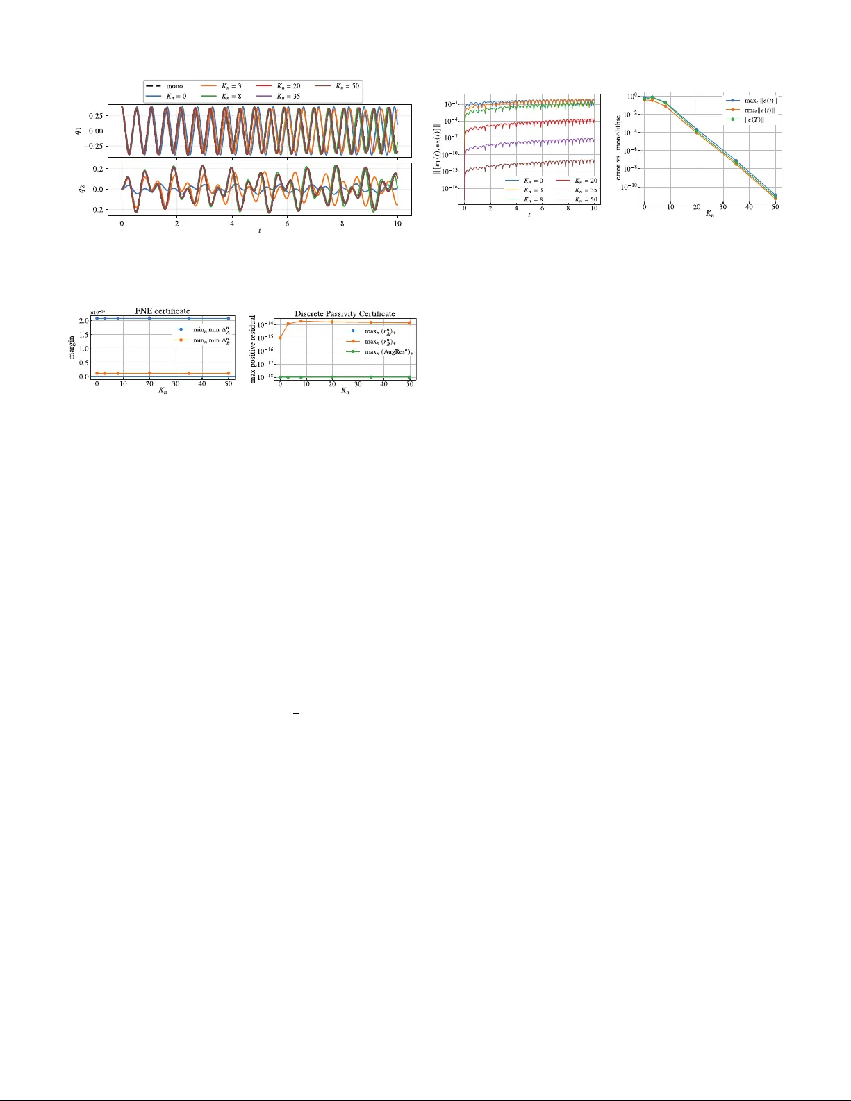
1 Early-T erminable Ener gy-Safe Iterati v e Coupling for P arallel Simulation of Port-Hamiltonian Systems Qi W ei, Jianfeng T ao, Hongyu Nie, W angtao T an Abstract —Parallel simulation and control of large-scale robotic systems often r ely on partitioned time stepping, yet finite-iteration coupling can inject spurious energy by violating power consis- tency—even when each subsystem is passive. This letter proposes a novel energy-safe, early-terminable iterative coupling for port- Hamiltonian subsystems by embedding a Douglas–Rachf ord (DR) splitting scheme in scattering (wav e) coordinates. The lossless interconnection is enforced as an orthogonal constraint in the wav e domain, while each subsystem contributes a discrete- time scattering port map induced by its one-step integrator . Under a discrete passivity condition on the subsystem time steps and a mild impedance-tuning condition, we pro ve an augmented-storage inequality certifying discrete passivity of the coupled macro-step f or any finite inner -iteration budget, with the remaining mismatch captur ed by an explicit residual. As the inner budget increases, the partitioned update conv erges to the monolithic discrete-time update induced by the same integrators, yielding a principled, adaptive accuracy–compute trade-off, supporting ener gy-consistent real-time parallel simu- lation under varying computational budgets. Experiments on a coupled-oscillator benchmark validate the passivity certificates at numerical r oundoff (on the order of 10e-14 in double pr ecision) and show that the reported RMS state error decays monotonically with increasing inner -iteration budgets, consistent with the hard- coupling limit. Index T erms —Simulation and Animation, Dynamics, Formal Methods in Robotics and A utomation. I . I N T R O D U C T I O N T HE simulation and control of modern robotic systems increasingly push computation to the limit, as seen in massiv ely parallel learning pipelines [1], [2], high-fidelity sim- ulation of stiff and structurally complex dynamics [3], [4], and microsecond-lev el latency budgets in high-rate online MPC [5], [6]. These pressures make model partitioning increasingly important for parallel, co-simulation-based ex ecution [7], [8], [9]. Once models are split, the bottleneck becomes the numerical interface: discrete e xchange (sample-and-hold, e xtrapolation, asynchrony , delay) can break power consistenc y and create coupling defects [10], [11], [12], yielding spurious energy injection (ef fecti ve negati ve damping) e ven when subsystems are passiv e [10], [13], [14]. An interface must therefore enforce an energy-safe contract, not merely reduce local error . Related work on partitioned interfaces spans non-iterative (explicit) and iterati ve schemes [15], [16], [9]: non-iterati ve zero-order-hold or extrapolation is attracti ve for real time Manuscript received January 16, 2026; accepted ;Date of publication ; This work was supported by the National Natural Science Foundation of China (Grant No. 52075320). The authors are with the School of Mechanical Engineering, Shanghai Jiao T ong Univ ersity , Shanghai 200240, China. (e-mail: jftao@sjtu.edu.cn) Digital Object Identifier but can drift or destabilize under stiff coupling [17], [18], [19], while macro-step iterations (Gauss–Seidel/Jacobi, relax- ation) improv e consistency [18], [19] but raise delicate finite- iteration stability questions [20]. A distinct class of non- iterativ e schemes is represented by T ransmission Line Mod- eling (TLM), which exploits physically moti vated time delays to decouple subsystems. TLM introduces physically motiv ated delays to break algebraic loops and preserve passivity [21], [22], [23]. Howe ver , fixed delays can distort high-frequency behavior and limit performance [24], [25], [26], motiv ating delay-free alternativ es or impedance tuning. Structure-preserving modeling mak es the interface an ex- plicit po wer contract: pH/Dirac formulations encode inter- connection as a po wer-conserving constraint [27], [28], [29], and ener gy-consistent time stepping is well de veloped for monolithic integration [27], [30], [29] but harder to retain under partitioned, iterati ve coupling (notably for D AEs and pHD AEs) [31], [29]. In port coordinates the coupling layer is an input–output map whose inequality quantifies equiv alent damping; this motiv ates energy-safe interface updates via operator-splitting compositions [31], [32], whose guarantees are typically asymptotic (or end-of-step), so finite intermediate iterates may still fail to remain physically admissible or passiv e. W av e (scattering) variables turn power coupling into passiv e message passing [33] and are closely related to TLM-style interfaces when explicit delays are introduced [21], [22], [23], [26]. Y et stif f delay-free algebraic loops often still require interface tuning in practice [34], [9], while operator- splitting methods pro vide asymptotic consistency guarantees but do not by themselv es yield a wave-domain, iterate-level energy accounting. This moti vates embedding splitting updates in scattering coordinates to obtain parallel coupling with a transparent energy certificate under finite inner iterations. In this letter , we propose an anytime (early-terminable) energy-safe coupling interface by embedding operator -splitting updates in scattering (wa ve) coordinates. At each macro- step, a Douglas–Rachford (DR) type inner iteration recon- ciles a lossless wav e coupling constraint with the discrete- time port behavior induced by the subsystem integrators, a principled, adaptiv e accuracy–compute trade-off together with an augmented-storage energy certificate under finite inner iterations. The main contrib utions are as follo ws: 1) An anytime energy-safe interface for parallel cou- pling: W e introduce a parallelizable iterative coupling inter- face in scattering (wa ve) variables, using a Douglas–Rachford (DR) inner-loop to enforce the lossless interconnection while remaining energy-safe at every finite iteration (Algorithm 1). 2) Finite-iteration passivity guarantee: For any finite 2 (resistive) (storage) (interaction) (control) Dirac structure/ Ideal interconnection Fig. 1. Port-based view of a pH interconnection. Storage S , dissipation R , control C , and interaction J exchange power through port variables ( e, f ) and are constrained by a Dirac structure D , representing an ideal lossless interconnection ( e ⊤ f = 0 ). inner-iteration b udget, we establish a discrete passivity cer- tificate for the macro-step update via an augmented storage function (Theorem 1). 3) Con vergence to the monolithic discr etization: As the inner-iteration b udget increases, the partitioned update prov ably con verges to the monolithic discrete-time update induced by the same inte grator , yielding a principled accurac y– compute trade-off (Theorem 2). The remainder of the letter is or ganized as follows: Sec- tion II states the subsystem and interconnection model; Sec- tion III presents the iterative coupling algorithm; Section IV establishes passivity and con vergence properties; Section V reports numerical experiments; and Section VI discusses in- sights, limitations, and future work. I I . P R O B L E M F O R M U L A T I O N A. P ort-Hamiltonian Robotic Subsystems W e consider a robotic system decomposed into N subsys- tems indexed by i ∈ { 1 , . . . , N } , each exchanging power with the rest of the system through a set of power ports. Let x i ( t ) ∈ R n i denote the state of subsystem i , and let H i : R n i → R be a continuously differentiable Hamiltonian representing its stored energy . W e model each subsystem in port-Hamiltonian form as ˙ x i =  J i ( x i ) − R i ( x i )  ∇ H i ( x i ) + G i ( x i ) e i , f i = G i ( x i ) ⊤ ∇ H i ( x i ) , (1) where e i ( t ) ∈ R m i and f i ( t ) ∈ R m i are the port variables (effort and flow), G i maps port efforts to state dynamics, and J i , R i encode internal interconnection and dissipation and satisfy J i ( x i ) ⊤ = − J i ( x i ) , R i ( x i ) ⊤ = R i ( x i ) ⪰ 0 . (2) The instantaneous power supplied through the ports is giv en by the standard pairing P i ( t ) := e i ( t ) ⊤ f i ( t ) . (3) Using (1)–(2), the ener gy balance of subsystem i satisfies ˙ H i ( x i ) = ∇ H i ( x i ) ⊤  J i ( x i ) − R i ( x i )  ∇ H i ( x i ) + ∇ H i ( x i ) ⊤ G i ( x i ) e i ≤ e ⊤ i f i , (4) which is the standard passivity property with storage H i and port variables ( e i , f i ) . This port abstraction enables modular partitioning and inter- connection without exposing internal subsystem coordinates. B. Inter connection as P ower-Conserving Constraints Fig.1 summarizes the port-based interconnection view adopted in this letter . T o assemble a full robotic system from subsystems, the port variables { ( e i , f i ) } N i =1 are constrained by an interconnection law that enforces power consistency across interfaces. W e express such interconnections as algebraic constraints acting only on port variables, without reference to the internal subsystem states. Let e := col( e 1 , . . . , e N ) ∈ R m tot and f := col( f 1 , . . . , f N ) ∈ R m tot , where m tot := P N i =1 m i is the total port dimension. The interconnection is described by a set of admissible port pairs ( e, f ) ∈ D ⊆ R m tot × R m tot , (5) which we assume to be a linear subspace encoding the network topology and sign con ventions. W e define lossless interconnec- tions as Dirac structures: define the symmetric bilinear form on port pairs by ⟨ ⟨ ( e, f ) , ( e ′ , f ′ ) ⟩ ⟩ := e ⊤ f ′ + e ′ ⊤ f , (6) and let D ⊥ denote the orthogonal complement of D with respect to (6). W e assume D is a (linear) Dirac structure , i.e., D = D ⊥ . (7) Intuitiv ely , power conservation corresponds to isotr opy ( D ⊆ D ⊥ ), while the Dirac condition (7) expresses a maximal power -conserving interconnection relation. Consequently , for any ( e, f ) ∈ D , we ha ve 0 = ⟨ ⟨ ( e, f ) , ( e, f ) ⟩ ⟩ = 2 e ⊤ f , i.e., power conser vation at the interconnection le vel: ⟨ e, f ⟩ := e ⊤ f = N X i =1 e ⊤ i f i = 0 , ∀ ( e, f ) ∈ D . (8) The ke y point is that D depends only on the coupling archi- tecture and ports, and not on the particular realization of each subsystem; this separation enables modular/parallel subsystem computation subject to ( e, f ) ∈ D . For con venience, we denote the aggre gated port pair by z := ( e, f ) . In a time-discretized (implicit) setting, enforcing (1) together with ( e, f ) ∈ D leads to a globally coupled algebraic system, whereas a partitioned solv e requires iterati ve port-le vel reconciliation to recov er consistency . Our goal is an interconnection iteration that remains anytime energy-safe under a finite inner budget and conv erges to the monolithic implicit update as the budget increases; in Section III we formulate this as a fixed-point consistency problem in scattering v ariables. I I I . P A S S I V I T Y - P R E S E RV I N G I T E R A T I V E C O U P L I N G W e design a port-le vel interface algorithm for parallel subsystem solves that preserves lossless po wer exchange. Fig. 2 illustrates the ov erall design objectiv e; specifically , our goal is twofold: (i) the interface remains energy-safe 3 (Dirac structure/ Ideal) parallel subsystem integrators parallel subsystem integrators Subsystem B Subsystem A Energy-Safe inner iteration Fig. 2. Parallel iterati ve coupling of port-Hamiltonian subsystems. A macro- step n performs parallel subsystem integration; an inner interf ace iteration enforces an ideal lossless interconnection D . The update is energy-safe for any finite number of inner iterations and conver ges to the monolithic update as the inner iterations increase. under any finite inner -loop budget, and (ii) increasing the budget drives the update tow ard the monolithic macro-step. T o this end, we combine scattering variables (for norm- preserving power exchange) with a Douglas–Rachford (DR) type splitting (for systematic parallel reconciliation of coupling consistency). W e present the two-subsystem case for clarity; the multiport/multisubsystem case follows by stacking the wa ve variables, with the lossless interconnection represented by an orthogonal coupling matrix P . A. Scattering Representation for Iterative Inter connection Direct iterations on ef fort/flow v ariables ( e i , f i ) are gen- erally energy-unsafe: intermediate iterates may violate the lossless interconnection constraints and inject spurious energy at the interface. W e therefore introduce scattering v ariables, which pro vide a po wer-consistent parametrization and a con- venient Euclidean metric for interface signals. For clarity , we focus on two subsystems A and B con- nected through a common power port of dimension m , i.e., e A , f A , e B , f B ∈ R m . For each subsystem i , and for a fixed impedance parameter γ > 0 , define the incoming and outgoing wa ve v ariables a i := e i + γ f i √ 2 γ , b i := e i − γ f i √ 2 γ . (9) The in verse relations are e i = r γ 2 ( a i + b i ) , f i = 1 √ 2 γ ( a i − b i ) . (10) In these coordinates, the port power takes the form P i = e ⊤ i f i = 1 2  ∥ a i ∥ 2 − ∥ b i ∥ 2  , (11) so that the incoming/outgoing wa ve magnitudes admit a direct power interpretation. Most importantly , linear lossless interconnections (Dirac structures; Section II-B, (7)) become linear constraints in scattering v ariables. For example, consider two subsystems A and B interconnected by e A = e B , f A + f B = 0 . (12) Substituting (10) yields the wa ve exchange a A = b B , a B = b A , (13) i.e., a component sw ap and therefore norm-preserving (ener gy- neutral). This observation underlies our scattering-based inter- face iteration. B. Coupling as a F ixed-P oint Pr oblem At each macro time step, interconnection enforcement is a consistency problem between a lossless coupling constraint and the (discrete-time) port beha vior induced by the subsys- tem integrators. Define the stacked incident/outgoing wa ves a :=  a A a B  ∈ R 2 m , b :=  b A b B  ∈ R 2 m . (14) For the standard two-subsystem interconnection (12)–(13), the coupling is the swap and can be written as a = P b, P :=  0 I I 0  , P ⊤ P = I . (15) More generally , we allow any power-preserving coupling a = P b with P orthogonal (covering linear Dirac interconnections; Section II-B, (7)). At macro-step n , freeze the subsystem states at x n A , x n B . The chosen one-step integrator induces frozen port maps in scattering variables, b i = S n i ( a i ) , i ∈ { A, B } , (16) and stack them as S n := diag( S n A , S n B ) : R 2 m → R 2 m . The monolithic interface condition at macro-step n is to find ( a, b ) such that both the frozen port relations and the coupling constraint hold: b = S n ( a ) , a = P b. (17) Eliminating a giv es the fixed-point equation b = S n ( P b ) (equiv alently , a = P S n ( a ) ), which motivates an inner iter - ation. C. Iterative Coupling Algorithm W e operate on two time scales: a macro-step index n for subsystem time stepping, and an inner iteration index k for enforcing port-lev el coupling consistenc y . For each subsystem i ∈ { A, B } , let Φ ∆ t i denote the one-step time-stepping map in scattering variables, i.e., ( x n +1 i , b n +1 i ) = Φ ∆ t i ( x n i , a n i ) . At macro-step n , the one-step integrators induce the frozen scattering port map S n = diag( S n A , S n B ) (16). Define the lifted wa ve pair ζ := col( a, b ) ∈ R 4 m and the coupling subspace C :=  ζ = col( a, b ) ∈ R 4 m : a = P b  , and let Π C denote the orthogonal projection onto C (Remark 1). W e enforce coupling consistency via a lifted Douglas–Rachford inner iteration: initialize ζ n, 0 = col( a n, 0 , b n, 0 ) and for k = 0 , 1 , . . . , K n − 1 , (parallel subsystem step) ˆ b n,k := S n ( a n,k ) , (lift) y n,k := col( a n,k , ˆ b n,k ) , (coupling projection) ˜ y n,k := Π C  2 y n,k − ζ n,k  , (DR update) ζ n,k +1 := ζ n,k + ˜ y n,k − y n,k . (18) where a n,k is the incident-wav e block of ζ n,k . Let ˆ b n,⋆ denote the last a vailable shadow from the inner-loop (i.e., ˆ b n,⋆ := ˆ b n,K n − 1 if K n ≥ 1 , and ˆ b n,⋆ := b n, 0 if K n = 0 ). W e then enforce lossless coupling for the macro-step input by setting a n := P ˆ b n,⋆ and recover ( e n i , f n i ) via (10). 4 Algorithm 1 The proposed iterati ve coupling algorithm Require: Initial states x 0 A , x 0 B ; initial outgoing wa ves b 0 A , b 0 B ; time step ∆ t ; coupling matrix P with P ⊤ P = I ; inner budgets K n (and optional tolerance ε > 0 ). Ensure: For each macro-step n : updated ( x n +1 i , b n +1 i ) for i ∈ { A, B } . 1: for n = 0 , 1 , 2 , . . . do 2: Freeze x n A , x n B and form S n = diag( S n A , S n B ) as in (16). 3: Initialize b n, 0 ← col( b n A , b n B ) , a n, 0 ← P b n, 0 , ζ n, 0 ← col( a n, 0 , b n, 0 ) , and ˆ b n,⋆ ← b n, 0 . (inner-loop / interface reconciliation) 4: for k = 0 , 1 , . . . , K n − 1 do 5: Perform one lifted DR step (18) to obtain ˆ b n,k and ζ n,k +1 . ▷ parallel subsystem e val. 6: ˆ b n,⋆ ← ˆ b n,k . 7: if ∥ ζ n,k +1 − ζ n,k ∥ ≤ ε then 8: break 9: end if 10: end for 11: Set coupled incident wa ves a n ← P ˆ b n,⋆ . (macr o-step / parallel subsystem solve) 12: for all i ∈ { A, B } do ▷ in parallel 13: ( x n +1 i , b n +1 i ) ← Φ ∆ t i ( x n i , a n i ) . 14: end for 15: end for Remark 1 (Closed-form coupling projection) . For the linear constraint a = P b with P ⊤ P = I , the projection Π C admits a closed form. In particular , for any ˆ a, ˆ b ∈ R 2 m , Π C  col(ˆ a, ˆ b )  = col  P ¯ b, ¯ b  , ¯ b := 1 2 ( ˆ b + P ⊤ ˆ a ) . Thus the coupling update is closed-form and inexpensi ve. Remark 2 (Connection to explicit interf aces) . The limit case K n = 0 (skipping the inner-loop) reduces to the e xplicit scattering interface a n = P col( b n A , b n B ) . Each inner step e v aluates S n A and S n B in parallel, and the coupling update is a small closed-form linear operation. D. Ener gy Interpr etation W av e v ariables provide a direct energy accounting: by (11), P i = 1 2 ( ∥ a i ∥ 2 − ∥ b i ∥ 2 ) . Since P is orthogonal, the coupling step a = P b is energy-neutral; thus any net energy beha vior in the inner-loop is due solely to the mismatch between the frozen port relation b = S n ( a ) and the coupling constraint. I V . P A S S I V I T Y A N D C O N V E R G E N C E P RO P E RT I E S This section establishes two main properties of the proposed iterativ e coupling. Under an y finite inner-iteration budget, the coupled macro-step update is energy-safe (discrete-passiv e) in an augmented-storage sense (Theorem 1). Moreover , as the inner-iteration budget increases, the resulting partitioned up- date con ver ges to the monolithic discrete-time update induced by the same subsystem integrators (Theorem 2). W e start from two standing conditions: an energy-safe subsystem integrator (Condition 1) and firm none xpansiveness (resolv ent form) of the frozen port maps (Condition 2). A. Setup and Standing Conditions W e work in finite-dimensional Euclidean spaces and use standard properties of firmly nonexpansi ve maps (resolvent representation) and Douglas–Rachford splitting (DRS). For two subsystems with port dimension m , define stacked wav es a = col( a A , a B ) ∈ R 2 m and b = col( b A , b B ) ∈ R 2 m , and define the stacked w av e pair ζ := col( a, b ) ∈ R 4 m , ∥ ζ ∥ 2 := ∥ a ∥ 2 + ∥ b ∥ 2 . (19) T o av oid confusion with Section II (where z := ( e, f ) denotes an effort/flo w port pair), we reserv e ζ for wav e pairs. Let the lossless coupling be a = P b with P ⊤ P = I (the scattering- domain representation of a linear Dirac interconnection; Sec- tion II-B, (7)), and define the associated linear subspace C := { ζ = col( a, b ) ∈ R 4 m : a = P b } . (20) At macro-step n , the chosen one-step integrator induces frozen port maps S n i : a i 7→ b i and S n = diag( S n A , S n B ) as in (16). Condition 1 (Energy-safe subsystem integrator) . F or each i ∈ { A, B } , the discr ete-time update map Φ ∆ t i satisfies, for all n , H i ( x n +1 i ) − H i ( x n i ) ≤ 1 2  ∥ a n i ∥ 2 − ∥ b n +1 i ∥ 2  , (21) wher e a n i is the incident wave used to advance subsystem i over the macro-step and b n +1 i is the r esulting outgoing wave. Remark 3 (Passi vity-preserving integrators satisfy Condi- tion) . Man y passi vity-preserving one-step methods for port- Hamiltonian systems enforce (21) in scattering coordinates by construction; here we simply treat (21) as a standing condition on the chosen subsystem integrators. Condition 2 (Frozen port maps are resolvents (FNE)) . At each macr o-step n , each fr ozen port map S n i : R m → R m is firmly nonexpansive (FNE) in the Euclidean norm: ∥ S n i ( α ) − S n i ( β ) ∥ 2 ≤ ⟨ S n i ( α ) − S n i ( β ) , α − β ⟩ , ∀ α, β ∈ R m . (22) In our scattering implementation, this property is enforced by a suitable choice of the impedance parameter γ ; see Proposition 1. Proposition 1 (A sufficient γ -rule for FNE (impedance bound)) . F ix n and a subsystem i ∈ { A, B } . Suppose the fr ozen discrete-time incremental port r elation induced by the chosen one-step inte grator can be written as δ e i = Z n i,d δ f i , with a symmetric matrix Z n i,d ⪰ 0 . Let S n i denote the induced fr ozen wave map for scattering impedance γ > 0 . If Z n i,d ⪰ γ I , then S n i is firmly nonexpansive (hence Condition 2 holds for subsystem i at macr o-step n ). Pr oof. With the scattering transform a = ( e + γ f ) / √ 2 γ and b = ( e − γ f ) / √ 2 γ , increments satisfy δ a = 1 √ 2 γ ( Z n i,d + γ I ) δ f i and δ b = 1 √ 2 γ ( Z n i,d − γ I ) δ f i , hence δ b = ( Z n i,d − γ I )( Z n i,d + γ I ) − 1 δ a. 5 If Z n i,d ⪰ γ I , then for e very eigen value λ ≥ γ of Z n i,d the corresponding eigen value of S n i is ( λ − γ ) / ( λ + γ ) ∈ [0 , 1] , so 0 ⪯ S n i ⪯ I . A self-adjoint linear map with spectrum in [0 , 1] is firmly nonexpansi ve [35]. Remark 4 ( γ as a tuning parameter) . Condition 2 is a property of the discr ete-time frozen port map and depends on the scattering impedance γ . Proposition 1 provides a conserv ativ e rule: selecting γ below a uniform lo wer bound on the incre- mental discrete impedance (e.g., γ ≤ inf n λ min ( Z n i,d ) on the relev ant trajectory set) guarantees FNE. In practice, (22) can be monitored via the empirical mar gin ∆ used in Section V ; persistent ne gativ e margins indicate that the chosen ( γ , ∆ t ) violates Condition 2. In the linear symmetric-impedance case, the bound Z n i,d ⪰ γ I is also necessary , hence if-and-only-if. B. Discr ete P assivity under Finite Iter ations Fix a macro-step n and consider the inner-loop of Sec- tion III-C. W e make explicit the distinction between the DR iterate (the object to which standard DRS theorems apply) and the coupling-consistent interface signal used to dri ve the macro-step update. Let ζ n,⋆ ∈ C denote a monolithic interface solution at macro-step n (not necessarily unique), i.e., a wav e pair satisfy- ing the coupling constraint and the frozen subsystem relations: ζ n,⋆ = col( a n,⋆ , b n,⋆ ) ∈ C , b n,⋆ = S n ( a n,⋆ ) . (23) Here “monolithic” means: for the same discrete-time inte gra- tors used to define S n i at macro-step n , both a = P b and b = S n ( a ) hold simultaneously . Under Condition 2, S n is firmly nonexpansi ve; hence there exists a maximal monotone operator A n on R 2 m such that S n = J A n := ( I + A n ) − 1 [35]. Eliminating a = P b in (23) yields the reduced macro-step interface condition for the stacked outgoing wav e b := col( b A , b B ) ∈ R 2 m : 0 ∈ A n ( b ) + ( I − P ) b. (24) Thus, at macro-step n the interface solve reduces to finding a zero of the sum of two maximal monotone operators, for which DRS applies. This reduced-coordinate DRS is alge- braically equiv alent to the lifted iteration (18), while being more conv enient for analysis. Let L := I − P , whose resolvent is J L = ( I + L ) − 1 = (2 I − P ) − 1 . Remark 5 (Monotonicity of the linear coupling operator) . For any orthogonal P , the linear map L := I − P is monotone since ⟨ x, Lx ⟩ = ∥ x ∥ 2 − ⟨ x, P x ⟩ ≥ ∥ x ∥ 2 − ∥ x ∥∥ P x ∥ = 0 , hence maximal monotone [35]. W e no w describe the DR iterate and its shadow . The v ariable u n,k is the DR iterate (an auxiliary trial input to the port map). Its shadow ˆ b n,k := J A n ( u n,k ) yields a coupling-consistent incident wave ˆ a n,k = P ˆ b n,k , which is the interface signal used to dri ve the macro-step update. Initialize u n, 0 ∈ R 2 m and generate the DRS iterates for (24): ˆ b n,k := J A n ( u n,k ) = S n ( u n,k ) , v n,k := J L  2 ˆ b n,k − u n,k  , u n,k +1 := u n,k + v n,k − ˆ b n,k . (25) Equiv alently , (25) defines a DRS operator T n DR via u n,k +1 = T n DR ( u n,k ) . The coupling-consistent wav e pair associated with ˆ b n,k is ˆ ζ n,k := col( P ˆ b n,k , ˆ b n,k ) ∈ C , ˆ a n,k := P ˆ b n,k . (26) In Algorithm 1, the subsystems are adv anced once using ˆ a n := P ˆ b n,⋆ , where ˆ b n,⋆ denotes the last a vailable shado w . Define the augmented storage at macro-step n (relative to the monolithic interface solution) as V n := H A ( x n A ) + H B ( x n B ) + 1 2 ∥ u n,K n − u n, † ∥ 2 , (27) where u n, † ∈ Fix( T n DR ) is a fixed point of the DRS operator associated with (25) (equiv alently , J A n ( u n, † ) = b n,⋆ is a monolithic interface solution). The additional term quantifies the inner-loop fixed-point residual and accounts for finite interface mismatch. Since J A n is firmly nonexpansi ve, the Fejér decrease of ∥ u n,k − u n, † ∥ also controls the shado w mismatch ∥ ˆ b n,k − b n,⋆ ∥ . Theorem 1 (Energy safety under finite inner iterations) . Suppose Condition 1 holds and the inner iteration (25) is executed for K n steps at macr o-step n , and the macr o-step update is driven by ˆ a n := P ˆ b n,⋆ , where ˆ b n,⋆ denotes the last available shadow . Under Condition 2 and the solvability condition that ζ n,⋆ exists, the coupled macr o-step update satisfies the inequality  H A ( x n +1 A ) + H B ( x n +1 B )  −  H A ( x n A ) + H B ( x n B )  + 1 2 ∥ u n,K n − u n, † ∥ 2 − 1 2 ∥ u n, 0 − u n, † ∥ 2 ≤ 1 2  ∥ ˆ a n ∥ 2 − ∥ b n +1 ∥ 2  . (28) In particular , any finite inner-loop mismatc h is accounted for by the decrease of the DRS fixed-point r esidual term 1 2 ∥ u n,k − u n, † ∥ 2 (a F ejér-monotone quantity), while the physical ener gy change is contr olled by the supplied wave power . Here b n +1 denotes the actual outgoing wave produced by advancing the subsystems once with input ˆ a n . If K n = 0 , we tak e ˆ b n,⋆ = b n, 0 . Pr oof. Fix n . Under Condition 2, S n is firmly none xpansiv e and hence there exists a maximal monotone operator A n such that S n = J A n [35]. Define L := I − P ; by Remark 5, L is maximal monotone. Let R A n := 2 J A n − I and R L := 2 J L − I ; since resolv ents are firmly nonexpansi ve, the reflections are nonexpansi ve and the Douglas–Rachford operator T n DR := 1 2  I + R L R A n  is firmly nonexpansi ve [35]. Since u n,k +1 = T n DR ( u n,k ) , firm nonexpansi veness implies Fejér monotonicity of the Picard iterates with respect to Fix( T n DR ) [35]: for an y u n, † ∈ Fix( T n DR ) , ∥ u n,k +1 − u n, † ∥ 2 ≤ ∥ u n,k − u n, † ∥ 2 , ∀ k . In particular , ∥ u n,K n − u n, † ∥ 2 − ∥ u n, 0 − u n, † ∥ 2 ≤ 0 . Next, apply Condition 1 to the macro-step update driven by ˆ a n and sum over i ∈ { A, B } :  H A ( x n +1 A ) + H B ( x n +1 B )  −  H A ( x n A ) + H B ( x n B )  ≤ 1 2  ∥ ˆ a n ∥ 2 − ∥ b n +1 ∥ 2  . Finally , add the Fejér decrease to obtain (28). 6 C. Har d-Coupling Limit Recovers the Monolithic Update W e next formalize the hard-coupling limit claim: as K n → ∞ , the inner loop makes the shadow interface signal conv erge to a monolithic interface, and the resulting partitioned macro- step recov ers the monolithic discrete-time update induced by the same discretization. In this subsection we additionally assume continuity of the one-step maps in the incident wa ve input (and continue to assume solv ability of the monolithic interface condition, i.e., e xistence of ζ n,⋆ ). Lemma 1 (Inner-loop con ver gence to the monolithic inter- face) . Under Condition 2 and the solvability condition that ζ n,⋆ exists, the DRS iterates u n,k in (25) con ver ge to a fixed point u n, † ∈ Fix( T n DR ) , and the shadow sequence ˆ b n,k := J A n ( u n,k ) con ver ges to a monolithic outgoing wave b n,⋆ solving (24) . Consequently , ˆ a n,k = P ˆ b n,k con verg es to a n,⋆ = P b n,⋆ . Pr oof. Under Condition 2, S n = J A n for some maximal monotone A n [35]. By Remark 5, L := I − P is maximal monotone. The standard Douglas–Rachford splitting con ver - gence theory for sums of maximal monotone operators there- fore applies [36], [37], yielding conv ergence of the DR iterates to a fix ed point and con ver gence of the shado w to a solution; in finite dimension, weak and strong conv ergence coincide. Theorem 2 (Hard-coupling limit recovers the monolithic discretization) . Assume Lemma 1 holds at each macr o-step n , and assume the one-step update maps Φ ∆ t i ar e continuous in their arguments ( x n i , a n i ) on the rele vant set of trajectories. Then, for any fixed finite horizon T = N ∆ t , if K n → ∞ for each n = 0 , . . . , N − 1 , the partitioned trajectory pr oduced by Algorithm 1 conver ges (step-by-step on the grid) to a monolithic discrete-time trajectory obtained by selecting a solution of (23) at eac h macr o-step. Pr oof. Fix a finite horizon T = N ∆ t . F or each macro-step n ∈ { 0 , . . . , N − 1 } , Lemma 1 giv es ˆ b n,⋆ → b n,⋆ (hence ˆ a n = P ˆ b n,⋆ → a n,⋆ ) as K n → ∞ . By continuity of Φ ∆ t i and induc- tion on n , the one-step update ( x n +1 i , b n +1 i ) = Φ ∆ t i ( x n i , ˆ a n ) con verges to the monolithic update at step n , yielding grid- pointwise conv ergence of the partitioned trajectory to the monolithic discrete-time trajectory ov er the horizon. Remark 6 (Nonuniqueness and solution selection) . If (23) admits multiple solutions at a macro-step, then the limiting interface/trajectory in the hard-coupling limit may depend on initialization and implicit selection by the inner iteration. Theorem 2 guarantees con vergence to a trajectory consistent with some solution selection; explicit selection mechanisms are left for future work (Section VI). V . E X P E R I M E N T S : T W O - O S C I L L A T O R B E N C H M A R K W e validate the iterativ e coupling frame work on a minimal yet nontri vial benchmark: tw o coupled oscillators split into two subsystems with one scattering port each. Nontri viality comes from a mixed Duffing–linear configuration: Subsystem A includes a stif f hardening spring nonlinearity , so the frozen discrete-time port maps are state-dependent and cannot be re- duced to a globally linear impedance bound. The experiments Subsystem A （ Duf fing Oscil l ator ） Subsystem B （ Linear Oscillator ） Iterative Coupling Inner Loop Fig. 3. Schematic of the two-oscillator benchmark. T ABLE I T WO - O S CI L L A T O R B E NC H M A RK PA R AM E T ER S A N D S I M UL A T I ON S E TT I N G S . Parameter V alue Parameter V alue m 1 8 . 0 m 2 4 . 0 k 1 100 k 2 50 c 1 0 c 2 0 k 12 120 c 12 0 . 05 k nl 8000 q 1 (0) 0 . 4 q 2 (0) 0 v 1 (0) = v 2 (0) 0 ∆ t 0 . 01 T 10 . 0 γ 0 . 4 K n { 0 , 3 , 8 , 20 , 35 , 50 } target three claims from Sections III–IV : (i) Condition 2 (FNE margins), (ii) the augmented-storage energy certificate under finite inner iterations (Theorem 1), and (iii) con ver gence to a monolithic reference trajectory as K n → ∞ (Theorem 2). A. Benchmark and settings. Fig. 3 depicts the subsystem decomposition and ports. Each subsystem exposes a single port ( e i , f i ) and is interfaced through scattering variables ( a i , b i ) (Section III-A); lossless coupling is enforced via a = P b with P the swap matrix (Section III-B). Both subsystems are time-discretized by a passivity-preserving, energy-consistent discrete-gradient one- step method, so Condition 1 holds by construction; for the lin- ear subsystem, this reduces to an implicit midpoint/trapezoidal update. All model and simulation parameters are listed in T able I. For the Duffing subsystem we treat γ as a design parameter (T able I) and verify Condition 2 numerically via the FNE margins reported in Fig. 5(a). Since the hardening Duffing spring has amplitude-dependent incremental stiffness ∆ F / ∆ q (due to the cubic term), the induced incremental behavior is state-dependent; thus we do not claim a trajectory-independent guarantee and instead v erify Condition 2 along the realized trajectories using a finite set of test pairs. B. Results and analysis. Fig. 4 compares the trajectories q 1 ( t ) and q 2 ( t ) for different inner-iteration budgets K n against a monolithic reference computed with the same passivity-preserving discrete-gradient time stepper and time step ∆ t . 7 Fig. 4. Trajectories ( q 1 , q 2 ) for different inner-iteration budgets K n and the monolithic reference. (a) (b) Fig. 5. T wo-oscillator certificates versus inner -iteration budget K n . (a) FNE certificate: worst-case numerically evaluated margins for Condition 2. (b) Discrete-passivity and augmented-storage diagnostics: positive-part sum- maries ( · ) + of the discrete-passivity residual (21) and the augmented-storage residual associated with (28). W e check Condition 2 at each macro-step n by freezing subsystem states when e valuating S n i and estimating the margin induced by (22) on a finite set of test pairs ( α , β ) . ∆ n i ( α, β ) := ⟨ S n i ( α ) − S n i ( β ) , α − β ⟩ − ∥ S n i ( α ) − S n i ( β ) ∥ 2 , (29) so (22) holds iff ∆ n i ( α, β ) ≥ 0 for all α, β . Fig. 5(a) reports min n min ∆ n i and the number of test pairs with ∆ n i < − tol ( tol = 10 − 12 ) for each inner-iteration budget; since the trajectory depends on K n , these margins also v ary with K n . For discrete passi vity , we monitor the residual induced by (21), r n i := ( H i ( x n +1 i ) − H i ( x n i )) − 1 2 ( ∥ a n i ∥ 2 − ∥ b n +1 i ∥ 2 ) , so Condition 1 holds at step n whenever r n i ≤ 0 ; Fig. 5(b) summarizes ( r n i ) + , together with the positi ve part of the augmented-storag e r esidual associated with (28) (Theorem 1), i.e., the quantity obtained by moving the right-hand side to the left. Finally , Fig. 6 shows that the reported RMS state error to the monolithic reference decreases monotonically ov er the tested budgets as K n increases, consistent with Theorem 2. In summary , for the selected γ , the FNE margins along the realized trajectories are numerically nonnegati ve (Fig. 5(a)), indicating that Condition 2 is consistent with the benchmark. The discrete-passi vity residuals and the augmented-storage residual are essentially nonpositiv e in the reported positiv e- part summaries (Fig. 5(b)), with any remaining positive part at numerical roundoff (on the order of 10 − 14 in double preci- sion), supporting the finite-iteration certificate of Theorem 1. Finally , increasing K n monotonically reduces the reported RMS state error and approaches the monolithic reference (Fig. 6), consistent with Theorem 2. (a) (b) Fig. 6. Hard-coupling limit validation (Theorem 2). (a) RMS state error versus time relativ e to the monolithic reference. (b) RMS error decay versus K n (monotonic over the tested budgets). V I . D I S C U S S I O N This letter frames iterativ e coupling of port-Hamiltonian subsystems as a numerical interface design problem solved by a Douglas–Rachford inner iteration in scattering coordinates. The resulting augmented-storage inequality provides an any- time (early-terminable) energy-safety certificate for any finite inner-iteration budget, while the hard-coupling limit recov ers the monolithic discrete-time update induced by the same subsystem integrators. V iewed as an e xplicit interface layer , the inner -iteration b udget becomes an adjustable knob for an adaptiv e accuracy–compute trade-off, supporting energy- consistent real-time parallel simulation under varying com- putational budgets. The scattering-domain formulation also resembles passive message passing, suggesting a composable route to distributed co-simulation and in-the-loop, large-scale model-based optimization/control workflo ws in which subsys- tems are e valuated in parallel while coupling consistency is reconciled with a certificate. More broadly , this perspective shifts interface stabilization from ad-hoc tuning heuristics tow ard certificate-dri ven numerical interf ace design grounded in operator splitting. Open directions include quantitative finite- K n state-error bounds, explicit solution selection when the monolithic interf ace admits multiple solutions, and adap- tiv e impedance/budget selection (including asynchronous and communication-aware e xtensions). R E F E R E N C E S [1] N. Rudin, D. Hoeller, P . Reist, and M. Hutter, “Learning to walk in minutes using massiv ely parallel deep reinforcement learning, ” in Confer ence on robot learning . PMLR, 2022, pp. 91–100. [2] V . Mak oviychuk, L. W awrzyniak, Y . Guo, M. Lu, K. Store y , M. Macklin, D. Hoeller, N. Rudin, A. Allshire, A. Handa et al. , “Isaac gym: High performance gpu-based physics simulation for robot learning, ” arXiv pr eprint arXiv:2108.10470 , 2021. [3] E. T odorov , T . Erez, and Y . T assa, “Mujoco: A physics engine for model- based control, ” in 2012 IEEE/RSJ international conference on intelligent r obots and systems . IEEE, 2012, pp. 5026–5033. [4] Y . Hu, L. Anderson, T .-M. Li, Q. Sun, N. Carr , J. Ragan-Kelle y , and F . Durand, “Difftaichi: Differentiable programming for physical simulation, ” arXiv preprint , 2019. [5] R. Grandia, F . Jenelten, S. Y ang, F . F arshidian, and M. Hutter , “Per - ceptiv e locomotion through nonlinear model-predictive control, ” IEEE T ransactions on Robotics , vol. 39, no. 5, pp. 3402–3421, 2023. [6] T . Salzmann, E. Kaufmann, J. Arrizabalaga, M. Pav one, D. Scaramuzza, and M. Ryll, “Real-time neural mpc: Deep learning model predictiv e control for quadrotors and agile robotic platforms, ” IEEE Robotics and Automation Letters , vol. 8, no. 4, pp. 2397–2404, 2023. 8 [7] D. Negrut, R. Serban, H. Mazhar, and T . Heyn, “Parallel computing in multibody system dynamics: why , when, and how , ” Journal of Computational and Nonlinear Dynamics , vol. 9, no. 4, p. 041007, 2014. [8] A. V . Papadopoulos and A. Le va, “ A model partitioning method based on dynamic decoupling for the efficient simulation of multibody systems, ” Multibody System Dynamics , vol. 34, no. 2, pp. 163–190, 2015. [9] B. Schweizer, P . Li, and D. Lu, “Explicit and implicit cosimulation methods: stability and conv ergence analysis for different solver cou- pling approaches, ” Journal of Computational and Nonlinear Dynamics , vol. 10, no. 5, p. 051007, 2015. [10] S. Sadjina, L. T . Kyllingstad, E. Pedersen, and S. Skjong, “Energy conservation and co-simulation: Background and challenges, ” in Pr o- ceedings of the 2024 International Conference on Bond Graph Modeling and Simulation (ICBGM’24)(San Diego, CA, USA, 1st–3r d July 2024) , 2024. [11] S. Sadjina, L. T . Kyllingstad, S. Skjong, and E. Pedersen, “Energy conservation and power bonds in co-simulations: non-iterativ e adaptive step size control and error estimation, ” Engineering with Computers , vol. 33, no. 3, pp. 607–620, 2017. [12] M. Benedikt, D. W atzenig, J. Zehetner, and A. Hofer , “Nepce-a nearly energy-preserving coupling element for weak-coupled problems and co-simulations, ” in COUPLED V : pr oceedings of the V International Confer ence on Computational Methods for Coupled Problems in Science and Engineering: . CIMNE, 2013, pp. 1021–1032. [13] F . González, S. Arbatani, A. Mohtat, and J. Kövecses, “Ener gy-leak monitoring and correction to enhance stability in the co-simulation of mechanical systems, ” Mechanism and Machine Theory , vol. 131, pp. 172–188, 2019. [14] B. Rodríguez, A. J. Rodríguez, B. Sputh, R. Pastorino, M. Á. Naya, and F . González, “Energy-based monitoring and correction to enhance the accuracy and stability of explicit co-simulation, ” Multibody System Dynamics , vol. 55, no. 1, pp. 103–136, 2022. [15] C. Gomes, C. Thule, D. Broman, P . G. Larsen, and H. V angheluwe, “Co-simulation: a surve y , ” ACM Computing Surveys (CSUR) , v ol. 51, no. 3, pp. 1–33, 2018. [16] T . Blochwitz, M. Otter, M. Arnold, C. Bausch, C. Clauß, H. Elmqvist, A. Junghanns, J. Mauss, M. Monteiro, T . Neidhold et al. , “The functional mockup interface for tool independent exchange of simulation models, ” in Pr oceedings of the 8th international Modelica conference . Linköping Univ ersity Press, 2011, pp. 105–114. [17] A. Peiret, F . González, J. Kövecses, and M. T eichmann, “Multibody system dynamics interface modelling for stable multirate co-simulation of multiphysics systems, ” Mechanism and Machine Theory , v ol. 127, pp. 52–72, 2018. [18] X. Dai, A. Raoofian, J. Kövecses, and M. T eichmann, “Model-based co- simulation of flexible mechanical systems with contacts using reduced interface models, ” IEEE Robotics and Automation Letters , vol. 9, no. 1, pp. 239–246, 2023. [19] A. Raoofian, X. Dai, and J. Kövecses, “Nonsmooth reduced interface models and their use in co-simulation of mechanical systems, ” Journal of Computational and Nonlinear Dynamics , vol. 19, no. 7, p. 071006, 2024. [20] B. Schweizer , P . Li, and D. Lu, “Implicit co-simulation methods: Stability and conv ergence analysis for solver coupling approaches with algebraic constraints, ” ZAMM-Journal of Applied Mathematics and Me- chanics/Zeitschrift für Angewandte Mathematik und Mechanik , vol. 96, no. 8, pp. 986–1012, 2016. [21] P . Krus, “Robust modelling using bi-lateral delay lines for high speed simulation of complex systems, ” in The International Symposium on Dynamic Pr oblems of Mechanics, Mar ch, 13 to 18, 2011 Mar esias Beach Hotel São Sebastião, São P aulo, Brazil , 2011. [22] R. Braun, “Multi-threaded distributed system simulations using bi-lateral delay lines, ” Ph.D. dissertation, Linkopings Univ ersitet (Sweden), 2013. [23] R. Braun and D. Fritzson, “Numerically rob ust co-simulation using transmission line modeling and the functional mock-up interface, ” Simulation , vol. 98, no. 11, pp. 1057–1070, 2022. [24] L. Barbierato, S. Steffen-V ogel, D. S. Schiera, E. Pons, L. Bottaccioli, A. Monti, and E. Patti, “Locally distributed digital real-time power sys- tem co-simulation via multi-phase distributed transmission line model, ” IEEE T ransactions on Industry Applications , vol. 60, no. 6, pp. 8137– 8146, 2024. [25] J. D. BUR TON, K. A. EDGE, and C. R. BURR O WS, “ Analysis of an electro-hydraulic position control serv o-system using transmission-line modelling (tlm), ” in Proceedings of the JFPS International Symposium on Fluid P ower , vol. 1993, no. 2. The Japan Fluid Power System Society , 1993, pp. 507–514. [26] R. Braun, R. Hällqvist, and D. Fritzson, “Transmission line modeling co-simulation with distributed delay-size control using steady-state iden- tification, ” Engineering with computers , vol. 40, no. 1, pp. 301–312, 2024. [27] E. Celledoni and E. H. Høiseth, “Energy-preserving and passi vity- consistent numerical discretization of port-hamiltonian systems, ” arXiv pr eprint arXiv:1706.08621 , 2017. [28] H. Parks and M. Leok, “V ariational integrators for interconnected lagrange–dirac systems, ” Journal of Nonlinear Science , vol. 27, no. 5, pp. 1399–1434, 2017. [29] M. Ehrhardt, M. Günther, and D. Šev ˇ covi ˇ c, “Structure-preserving cou- pling and decoupling of port-hamiltonian systems, ” arXiv preprint arXiv:2511.20150 , 2025. [30] F . J. Argus, C. P . Bradley , and P . J. Hunter , “Theory and implementation of coupled port-hamiltonian continuum and lumped parameter models, ” Journal of Elasticity , vol. 145, no. 1, pp. 339–382, 2021. [31] A. Bartel, M. Günther , B. Jacob, and T . Reis, “Operator splitting based dynamic iteration for linear differential-algebraic port-hamiltonian systems, ” Numerische Mathematik , vol. 155, no. 1, pp. 1–34, 2023. [32] A. Bartel, M. Diab, A. Frommer , M. Günther, and N. Marheineke, “Split- ting techniques for daes with port-hamiltonian applications, ” Applied Numerical Mathematics , vol. 214, pp. 28–53, 2025. [33] J. Cervera, A. J. van der Schaft, and A. Baños, “Interconnection of port- hamiltonian systems and composition of dirac structures, ” Automatica , vol. 43, no. 2, pp. 212–225, 2007. [34] W . Chen, S. Ran, C. W u, and B. Jacobson, “Explicit parallel co- simulation approach: analysis and improved coupling method based on h-infinity synthesis, ” Multibody System Dynamics , vol. 52, no. 3, pp. 255–279, 2021. [35] H. H. Bauschke and P . L. Combettes, Conve x Analysis and Monotone Operator Theory in Hilbert Spaces , 2nd ed. Cham: Springer , 2017. [36] P .-L. Lions and B. Mercier , “Splitting algorithms for the sum of tw o nonlinear operators, ” SIAM Journal on Numerical Analysis , vol. 16, no. 6, pp. 964–979, 1979. [37] B. F . Svaiter , “On weak conver gence of the douglas–rachford method, ” SIAM Journal on Contr ol and Optimization , vol. 49, no. 1, pp. 280–287, 2011.