Critical Self-Similar Markov Trees

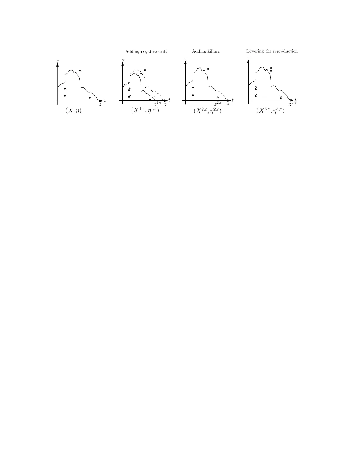
Critical Self-Similar Mark o v T rees Nicolas Curien ∗ , Xing jian Hu † and Dong jian Qian ‡ Abstract Recen tly in tro duced and studied in [ BCR25 ], a self-similar Mark ov tree (ssMt) is a random decorated tree that v astly generalises the fragmen tation tree. W e study here the critic al c ase that was left aside in [ BCR25 ]. Borro wing tec hniques from branching random w alk, in particular the recen t result of Aïdék on–Hu–Shi [ AHS25 ], w e can com- plete the picture by constructing critical ssMt, computing their fractal d imension and studying their asso ciated harmonic and length measures using spinal decomp osition. 1 In tro duction Self-similar Mark o v trees ha v e recen tly b een in tro duced in [ BCR25 ]. They can b e seen as generalisations of the fragmen tation trees of Haas & Miermon t [ HM04 ], or as the genealogical trees underlying the Lamp erti transformation of branc hing Lévy pro cesses [ BM19 ]. They encompass and unify v arious mo dels including Aldous’ famous Brownian Contin uum Random tree [ Ald91 ] and its stable generalisations [ Duq02 ] as w ell as more exotic trees such as the Bro wnian Cactus [ CLGM13 ] sitting inside the Brownian sphere [ LGR20 , BCK18 ], or the scaling limits of p eeling or parking trees [ BBCK18 , CC25 ]. They are conjectured to describ e scaling limits of multi-t yp e Biena ymé–Galton–W atson trees, exactly as Lamp erti’s self-similar Mark ov pro cesses describ e the scaling limits of p ositiv e Mark ov c hains on the integers. Their cen tral role in the theory of random tree spark ed a recen t in terest, see e.g. [ BRR O26 , CFT25 ] for their in trinsic studies or [ ADS22 , LGR20 , BCK18 , DSPW25 ] for their connections with v arious mo dels of random planar geometry . F ormally , a self-similar Mark o v tree (ssMt) is a family of laws ( Q x : x > 0) of decorated con tinuous random R -trees T = ( T , d T , ρ, g ) where ρ is the ro ot of the tree and g : T → R + ∗ Univ ersité Paris-Sacla y , nicolas.curien@universite- paris- saclay.fr † F udan Universit y , xjhu22@m.fudan.edu.cn ‡ F udan Universit y , djqian22@m.fudan.edu.cn 1 is a real decoration whic h is upp er semi-contin uous (usc) on T and p ositiv e on its skeleton. Under the la w Q x , the random decorated tree T starts from the initial decoration g ( ρ ) = x and enjo ys the follo wing t w o ep on ymic prop erties: 1. Mark ov prop ert y . F or eac h h > 0 , conditioned on the subtree truncated at heigh t h , the decorated subtrees ab ov e h are indep enden t of eac h other and hav e law Q y if the decoration at its ro ot is y . 2. Self-similarit y . There exists α > 0 , the self-similar index , suc h that for each x > 0 , the tree ( T , d T , ρ, g ) under Q x has the same law as ( T , x α d T , ρ, x · g ) under Q 1 . F ollo wing [ BCR25 , Section 2], a self-similar Mark ov tree can b e describ ed by its c haracteristic quadruplet ( σ 2 , a , Λ ; α ) , whic h through a Lamp erti transformation encapsulates the la w of their underlying branc hing Lévy pro cesses. In particular, the generalised Lévy measure Λ is a (p ossibly inﬁnite) measure on the space S = { u = ( u 0 , u 1 , ... ) : u 0 ∈ R and u 1 ≥ u 2 ≥ ... ∈ R ∪ {−∞}} whic h describ es the splitting rules: Informally , the ssMt is the genealogical tree of a system of individuals evolving indep enden tly of each other, and where an individual of decoration x > 0 sees its decoration instantaneously mo v ed to x · e y 0 while giving rise to a family of new individuals with decorations x · e y 1 , x · e y 2 , ... (whic h are interpreted as the birth of new individuals) x → ( x · e y 0 , ( x · e y 1 , x · e y 2 , · · · )) at a rate x − α · Λ (d y ) , (1.1) where α > 0 is the self-similarit y parameter. The pro jection Λ 0 of Λ on its ﬁrst co ordinate is required to b e a Lévy measure, and its pro jection Λ 1 on to the second co ordinate satisﬁes a mild integrabilit y assumption (see ( 2.1 )). The co eﬃcien t a ∈ R enco des the drift term while σ 2 con trols the Brownian part of the ev olution of the decoration along branc hes. See Section 2.1 or [ BCR25 ] for details. When the starting decoration x > 0 is ﬁxed, the law Q x is the distribution of the ab o ve genealogical tree started with an individual of decoration x . A crucial quan tit y to consider is the cumulan t function deﬁned by κ ( γ ) = 1 2 σ 2 γ 2 + a γ + Z S Λ (d u ) e γ u 0 − 1 − γ u 0 1 {| u 0 |≤ 1 } + ∞ X i =1 e γ u i ! , = ψ ( γ ) + Z S Λ (d u ) ∞ X i =1 e γ u i ! (1.2) where ψ ( γ ) is the Laplace exp onen t of the Lévy pro cess with characteristics ( σ 2 , a , Λ 0 ) . This function κ also app ears as the Biggins transform of the underlying branching Lévy pro cess. 2 Figure 1: Illustration of the criticality on the cumulant function. In particular, if κ tak es strictly negativ e v alues then the t yp es of individuals is deca ying o ver generations in exp ectation, and the genealogical tree of the ab ov e system of particles is compact and provides a ssMt. While if κ only takes p ositiv e v alues then the tree explo des lo cally , see [ BS16 ]. The case when κ touches 0 while remaining non-negative was left aside in [ BCR25 ] and is the context of this pap er: Assumption 1.1 (Criticality I) . Supp ose that for γ ≥ 0 we have κ ( γ ) ≥ 0 and ther e exists ω − ≥ 0 such that κ ( ω − ) = 0 and κ is twic e diﬀer entiable at ω − . F urthermor e, Ther e exists γ 1 > ω − such that ψ ( γ 1 ) < 0 and κ ( γ 1 ) < ∞ . W e shall hav e a stronger technical Assumption 3.5 analogue to the Cramér assumption in [ BCR25 ] needed to study ﬁne properties of ssMt. This assumption is omitted in the in tro duction for readability . Theorem 1.2 (Construction of the critical ssMt) . Under A ssumption 1.1 the c onstruction in [ BCR25 ] c an inde e d b e p erforme d and it yields a family of laws ( Q x ) of c omp act de c o- r ate d r andom tr e es satisfying the Markov and self-similarity pr op erty. F urthermor e, under A ssumption 3.5 , for any x > 0 the Hausdorﬀ dimension of the le aves ∂ T of a tr e e T under Q x is a.s. dim H ( ∂ T ) = ω − α . Compared to [ BCR25 ], the construction of self-similar Marko v trees in the critical case relies on the v ery recent result of Aïdék on–Hu–Shi [ AHS25 ] which w as in fact motiv ated b y the ab o ve application. A few critical ssMt w ere already considered in [ BCR25 ] but their existence was prov ed case-by-case using sp eciﬁc features of the mo dels. This w as notably the case for the ssMt of Aïdékon and Da Silv a [ ADS22 ] whic h arose from half-planar Brownian excursion. With the critical case at hand, the family of ssMt, whic h is now complete, is conjectured to describ e all p ossible scaling limits of multi-t yp e Bienaymé–Galton–W atson trees. W e now mov e on to discuss the prop erties of critical self-similar Mark ov trees and their natural measures following the same strategy as for the sub critical case [ BCR25 ]. 3 Measures and spine decomp osition. An y decorated tree T = ( T , g ) carries a natural Leb esgue measure λ T on its sk eleton, and the length measures are obtained b y using the decoration g as density . F ormally , for an y γ ≥ 0 , we deﬁne the γ -length measure on T as d λ γ := g γ − α · d λ T . In the sub critical case, those measures are deﬁned as so on as γ > ω − and Prop osition 2.12 of [ BCR25 ] even ensures that λ γ has ﬁnite exp ected mass when κ ( γ ) < 0 . In the critical case, w e pro ve in Section 3 that λ γ is still a ﬁnite measure when γ > ω − a.s. but with inﬁnite exp e cte d length . Let us now turn to the equiv alent of the harmonic measure of [ BCR25 , Chapter 2.3.3]. Recall from Assumption 1.1 that κ ( ω − ) = 0 . In this case, the pro cess W n = X | u | = n ( χ ( u )) ω − , where χ ( u ) are the initial decorations of the individuals app earing in the genealogical tree (indexed by the Ulam’s tree, see the construction of ssMt in Section 2.1 ) is a martingale. In the con text of branching random walks, suc h a martingale is called an additiv e martingale. In the critical case, although p ositiv e, this martingale has a trivial limit (see [ Shi16 , Theorem 3.3]), so the construction of the harmonic measure from [ BCR25 ] needs to b e adapted. The standard w a y to remedy this problem is to consider the deriv ativ e martingale deﬁned b y D n = − X | u | = n ( χ ( u )) ω − log( χ ( u )) . (1.3) Standard results in the ﬁeld of branc hing random w alks (see [ Shi16 , Section 5]) ensures con vergence of the deriv ativ e martingale tow ards a non-trivial p ositiv e limit D ∞ . This enables us to endow the ssMt T with a non-trivial measure µ of mass D ∞ whic h pla ys the role of the harmonic measure in the sub critical case (we keep the same name in our context). Although not immediate from the deﬁnition, w e will sho w that the harmonic measure µ is intrinsic, i.e. measurable with resp ect to the decorated tree only (as opp osed to its genealogical represen tation). In fact µ can b e obtained as a limit of the (in trinsic) length measures λ γ when γ ↓ ω − lim γ ↓ ω − κ ′′ ( ω − ) 2 ( γ − ω − ) λ γ = µ, at least along a subsequence as it was the case in the sub critical case [ BCR25 , Prop osition 2.15] (see Theorem 4.4 for details). This con vergence represents the most tec hnical part of this w ork and requires delicate truncation estimates and ﬂuctuation iden tities for Lévy pro cesses. 4 As in [ BCR25 , Chapter 4 ] those random measures are used to p erform spinal decomp o- sition of the underlying ssMt. The spinal decomp osition originates in the setting of branching random walks and generalises to man y diﬀerent genealogical mo dels, suc h as branching Lévy pro cesses and self-similar Marko v trees. When doing so, w e wan t to deal with the la w of the decorated tree T together with a mark ed p oint r sampled from the harmonic (or length) measure. The line segment b et ween the ro ot ρ and the marked p oin t r is called the spine. The spinal decomp osition theorem describ es the la w of the spine and the la w of the subtrees dangling to the spine. In the critical case, the harmonic or length measures ha ve inﬁnite exp ected total mass, so w e cannot directly bias the law of the tree b y sampling a p oint ac- cording to those measures. Ho w ev er, this can b e p erformed after a conv enien t cut-oﬀ on the decoration, see Theorem 4.1 in Section 4.1 . In particular, in contrast to [ BCR25 ], the Lévy pro cesses con trolling the evolution of the decoration along the spine are now conditioned to sta y b elo w a barrier. The spinal decomp osition is profound and has man y applications. The rest of the pap er is organised as follo ws. In section 2, after a quic k recap of the construction in [ BCR25 ] w e apply the results of [ AHS25 ] to construct critical self-similar Mark ov trees. W e then imp ort man y results from the subcritical case using a "con tinuit y argumen t" since critical ssMt can, after a slight p erturbation, b e transformed in to a sub critical ssMt. This is used in particular to obtain a low er b ound on their Hausdorﬀ dimension, the spinal decomp osition and characterisation of bifurcators. In section 3, w e discuss the length and harmonic measures. A k ey idea imp orted from branc hing random walks is to consider the tree conditioned to stay b elo w a barrier. In section 4, w e present the spinal decomp osition theorem with resp ect to the truncated har monic measure. Section 5, perhaps the most tec hnical part of this pap er, is dev oted to analysing the relations b et w een harmonic and lengths measures (Theorem 4.4 ). A ckno wledgmen ts. W e thank Elie Aïdék on, Y ueyun Hu, and Zhan Shi for stimulating discussions around [ AHS25 ] as well as Jean Bertoin and Armand Riera. The last tw o au- thors w ere supp orted by the China Sc holarship Council. The ﬁrst author is supported b y "SuP erGRandMa", the ER C Consolidator Gran t No 101087572. Con ten ts 1 In tro duction 1 2 Bac kground and construction of ssMt 6 2.1 Background . . . . . . . . . . . . . . . . . . . . . . . . . . . . . . . . . . . . 6 5 2.2 Critical self-similar Marko v trees . . . . . . . . . . . . . . . . . . . . . . . . 9 2.3 Approximation by sub critical ssMt . . . . . . . . . . . . . . . . . . . . . . . 11 2.4 Examples . . . . . . . . . . . . . . . . . . . . . . . . . . . . . . . . . . . . . 14 3 Measures on critical ssMt 15 3.1 T o ols from Branc hing pro cesses . . . . . . . . . . . . . . . . . . . . . . . . . 15 3.2 Fluctuation theory for the Lévy pro cess ˆ ξ . . . . . . . . . . . . . . . . . . . . 17 3.3 Length measure of the tree b elow a barrier . . . . . . . . . . . . . . . . . . . 18 3.4 The harmonic measure . . . . . . . . . . . . . . . . . . . . . . . . . . . . . . 20 3.5 The Hausdorﬀ dimension of the leav es . . . . . . . . . . . . . . . . . . . . . 23 4 Prop erties of critical ssMt 25 4.1 Spinal Decomp osition and bifurcators . . . . . . . . . . . . . . . . . . . . . . 26 4.1.1 The spinal decomp osition theorem . . . . . . . . . . . . . . . . . . . 26 4.1.2 Pro of of the spinal decomp osition theorem. . . . . . . . . . . . . . . . 27 4.1.3 Bifurcators . . . . . . . . . . . . . . . . . . . . . . . . . . . . . . . . 30 4.2 Conv ergence from length measures to the harmonic measure. . . . . . . . . 31 4.2.1 More on the exp ected length . . . . . . . . . . . . . . . . . . . . . . . 35 4.2.2 Pro of of Lemma 4.8 : go o d and bad branc hes . . . . . . . . . . . . . . 37 2 Bac kground and construction of ssMt In this section we quickly recap the construction of decorated random trees by gluing dec- orated branches and pro v e the existence of critical self-similar Marko v trees (Theorem 1.2 ). F or more details, the reader is referred to [ BCR25 , Chapters 1,2]. 2.1 Bac kground W e ﬁrst recall the deﬁnition of characteristic quadruplet ( σ 2 , a , Λ ; α ) . Let S = [ −∞ , ∞ ) × S 1 where S 1 is the set of non-increasing sequences y = ( y 1 , y 2 , · · · ) with y i ∈ [ −∞ , ∞ ) and lim n →∞ y n = −∞ . W e require that Λ is a generalised Lévy measure on the space S , i.e., its pro jection Λ 0 to the ﬁrst co ordinate is a Lévy measure and Λ 1 to the second co ordinate satisﬁes Λ 1 ( { e y 1 > ε } ) < ∞ , ∀ ε > 0 . (2.1) The four entries ha ve sp eciﬁc meanings in the construction. The tuple ( σ 2 , a , Λ 0 ) charac- terises a Lévy pro cess which is the input of the decoration. The measure Λ 1 is the in tensity 6 of the birth even t. The parameter α > 0 is the self-similarity index . Given ( σ 2 , a , Λ ; α ) , w e ﬁrst construct the law of decoration-repro duction pro cess. Then the law of suc h pro cess induces a family of decorated branc hes indexed by the Ulam’s tree. Finally , through a glu- ing pro cedure w e build a decorated tree which is called the self-similar Mark ov tree with quadruplet ( σ 2 , a , Λ ; α ) . Decoration-repro duction pro cesses. A decoration-repro duction pro cess is a pair of pro cesses ( f , η ) where f is a non-negative right contin uous with left limits (rcll) pro cess on a line segment [ 0 , z ] called the decoration pro cess and where η is a p oint pro cess on [0 , z ] called the repro duction pro cess. Denote by P x the law of ( f , η ) with f (0) = x . W e sa y that the family ( P x ) x ≥ 0 is self-similar with index α > 0 if for eac h x > 0 , the la w P x coincides with the rescaled pair ( f ( x ) , η ( x ) ) = F α x ( f , η ) under P 1 where f ( x ) : [0 , x α z ] → [0 , ∞ ) , f ( x ) ( t ) = xf ( x − α t ) (2.2) and η ( x ) is the push-forw ard of η under the map [0 , z ] × (0 , ∞ ) → [0 , x α z ] × (0 , ∞ ) , ( t, y ) 7→ ( x α t, xy ) . W e construct suc h a family ( P x ) x> 0 using c haracteristic quadruplet ( σ 2 , a , Λ ; α ) as follows: Let N = N (d t, d y , d y ) b e a Poisson random measure on [0 , ∞ ) × S with intensit y d t Λ (d y , d y ) . Denote b y N 0 (d t, d y ) its pro jection to the ﬁrst and the second co ordinates and b y N 1 = N 1 (d t, d y ) its pro jection to the ﬁrst and the third co ordinates. Let B b e a standard Bro wnian motion starting from 0 indep enden t of N . Construct a pro cess ( ξ ( t )) t ≥ 0 b y ξ ( t ) = σ B ( t ) + a t + Z [0 ,t ] × R y 1 {| y | > 1 } N 0 (d t, d y ) + Z [0 ,t ] × R y 1 {| y |≤ 1 } N c 0 (d t, d y ) . The comp ensate p oin t pro cess is deﬁned by N c 0 (d t, d y ) := N 0 (d t, d y ) − d t Λ 0 (d y ) . The pro cess ( ξ ( t )) t ≥ 0 is a Lévy pro cess with life-time ζ := inf { t > 0 : ξ ( t ) = −∞} . W e may consider the Lévy pro cess ξ started from b ∈ R by adding a constant b to the display ab o v e. Deﬁne its Laplace exp onen t ψ ( γ ) by the following equation 1 E [exp( γ ξ ( t ))] = E [ exp( γ ξ ( t )) · 1 { t<ζ } ] = exp( tψ ( γ )) , γ > 0 . (2.3) By the Lévy Khintc hine form ula, w e hav e ( R ∗ := R ∪ {−∞} ) ψ ( γ ) = 1 2 σ 2 γ 2 + a γ + Z R ∗ (e γ y − 1 − γ y 1 | y |≤ 1 )Λ 0 (d y ) . (2.4) 1 Suc h exp ectation could b e inﬁnite in general. The condition that ψ ( γ ) < ∞ is included in the sub critical and critical condition in the next section. 7 W e next apply the Lamp erti transformation to the pro cess ( ξ ( t )) t ≥ 0 . Consider the time c hange ϵ ( t ) := Z t 0 exp( αξ ( s ))d s for 0 ≤ t ≤ ζ , z = ϵ ( ζ − ) = Z ζ 0 exp( αξ ( s ))d s. The (random) function ϵ ( t ) : [0 , ζ ) → [0 , z ) is a bijection a.s.. W rite τ as the recipro cal bijection so that a.s. R τ ( t ) 0 exp( αξ ( s ))d s = t . By the Lamp erti transformation the pro cess ( X ( t ) := exp( ξ ( τ ( t )))) t ∈ [0 ,z ) is a p ositiv e self-similar Marko v pro cess (pssMp) starting from 1 with scaling exp onen t α . Sp eciﬁcally , for each x > 0 , the scaled pro cess ( xX ( x − α t )) t ∈ [0 ,x α z ) has the same law as X starting from x . The p oin t 0 serv es as a cemetery p oin t for X . W e alw ays set X ( z ) := 0 when z < ∞ such that X is a rcll pro cess. W e deﬁne the repro duction pro cess η using the other pro jection N 1 (d t, d y ) . W e rewrite eac h atom ( s, y ) of N 1 (p ossibly rep eated according to their m ultiplicities), as pairs ( s, y ℓ ) ℓ ≥ 1 when y  = ( −∞ , −∞ , . . . ) . Recall the exp onen tial functional ϵ ( t ) . Set η := X 1 { ϵ ( s ) ≤ z } δ ( ϵ ( s ) , exp( ξ ( s − )+ y l )) , (2.5) where δ ( t,x ) is the Dirac measure at ( t, x ) and the sum is tak en ov er all the pairs ( s, y ℓ ) ℓ ≥ 1 . Denote the law of ( X , η ) by P x if X starts from x . W e see that the family ( P x ) x> 0 is self-similar with parameter α . F or brevit y , w e write P for P 1 . Decorated-repro duction family . Let U = S n ≥ 0 ( N ∗ ) n b e the Ulam tree with the conv en- tion ( N ∗ ) 0 = { ∅ } . Set U ∗ = U \{ ∅ } . The lea v es of the Ulam tree are denoted by ∂ U := N N . W e write | u | = n (resp. | u | = ∞ ) if u ∈ ( N ∗ ) n (resp. u ∈ ∂ U ) for the generation of u , u − for the parent of u , uv for concatenation of u and v , and u k for the ancestor of u at generation k . With the family ( P x ) x> 0 , w e construct the decorated-repro duction family , which is a ran- dom family of decoration-repro duction pro cesses ( f u , η u ) u ∈ U . It is a particle system where eac h u is an individual (p ossibly ﬁctitious) and ( f u , η u ) describ es the trait and birth even t along its life. Eac h particle u is assigned a type χ ( u ) . By conv ention, w e set χ ( u ) = 0 if an individual is ﬁctitious. A t generation 0 , there is an individual with type χ ( ∅ ) = x > 0 . W e then sample ( f ∅ , η ∅ ) under P x . W e enumerate the atoms of η ∅ b y ( t 1 , y 1 ) , ( t 2 , y 2 ) , . . . , and complete the sequence with ﬁctitious individuals to get an inﬁnite sequence. The in- dividuals in the ﬁrst generation ha v e t yp es χ ( i ) = y i . Inductiv ely , for each u ∈ U with t yp e χ ( u ) , sample ( f u , η u ) under the la w P χ ( u ) indep enden tly . W e then set χ ( ui ) = y ui for i ∈ N as the t yp es of c hildren of u , where ( t u 1 , y u 1 ) , ( t u 2 , y u 2 ) , . . . are the atoms of η χ ( u ) . W e rep eat this pro cedure to obtain the next generation by using independent decoration- repro duction pro cesses for diﬀerent individuals. W e denote by P x the law of the family of 8 decoration-repro duction pro cesses ( f u , η u ) u ∈ U when the ancestor ∅ has the t yp e x and E x the corresp onding exp ectation. F or brevity , w e write P for P 1 and E for E 1 . Construct trees b y gluing branches. Let ( f u , η u ) u ∈ U b e a family of decoration- repro duction pro cesses. F or each individual u ∈ U , we view the decoration pro cess ( f u , η u ) as a decorated branc h ([ 0 , z u ] , d, 0 , f u ) with marks t ui (recall that ( t ui , y ui ) are atoms of η u and z u the lifetime of f u ). The distance d is the Euclidean distance. Let T 0 = ([0 , z ∅ ] , d, 0 , f ∅ ) . Induc- tiv ely , w e let T n +1 b e the decorated trees obtained from gluing the branc hes ([0 , z u ] , d, 0 , f u ) with | u | = n + 1 on to T n at the corresp onding t u lying in T n . The gluing op eration leads to a limiting metric space ( T , d T , ρ ) with a decoration function g as n → ∞ . F or eac h p oin t x in T , we set g ( x ) = sup f u ( x u ) where the suprem um is taken ov er x u in the branc h indexed b y u ∈ U identiﬁed to x . The following lemma provides a suﬃcien t condition for the space ( T , d T , ρ, g ) to b e a compact decorated real tree (see also [ Sé22 , Section 2]). Deﬁne the norm || f u || := z u + sup 0 ≤ t ≤ z u f u ( t ) . W e say that ( x i , i ∈ I ) is a n ull family if for ε > 0 , there are only ﬁnitely man y x i > ε . Lemma 2.1 ([ BCR25 , Lemma 1.5] Compactly glueable) . Supp ose that the family ( f u , η u ) satisﬁes ( || f u || , u ∈ U ) is a nul l family and lim k →∞ sup ¯ u ∈ ∂ U ∞ X n = k z ¯ u ( k ) = 0 . (2.6) Then ( T , d T , ρ, g ) is a c omp act de c or ate d r e al tr e e. T op ology of the space of (measured) decorated trees . W e close this section with a brief note on the top ology on the space of decorated compact real tree, see [ BCR25 , Section 1.4]. W e sa y T := ( T , d T , ρ, g ) and T ′ := ( T ′ , d ′ T , ρ ′ , g ′ ) are isomorphic if there exists a bijectiv e isometry ϕ : ( T , d T ) → ( T ′ , d ′ T ) suc h that ϕ ( ρ ) = ρ ′ and g ′ = g ◦ ϕ − 1 . Denote by T (resp. T • or T m ) the space of equiv alence (up to isomorphisms) classes of decorated compact real trees (resp. with an additional p oin t, or a ﬁnite Borel measure). W e alwa ys abuse T = ( T , d T , ρ, g ) or T • = ( T , d T , ρ, g , r ) to represen t an equiv alence class in the sequel (where r is an additional p oin t), since the quantities and prop erties we will consider are in v arian t under isomorphisms. These spaces are endow ed with d T , d T • , d T m , which are adaptations of the Gromov-Hausdorﬀ- p oin ted/Prokhorov distances that also take the decorations in to accoun t as hypographs. They are all P olish spaces. See [ BCR25 , Section 1.4] for details. 2.2 Critical self-similar Mark o v trees F or a generic choice of quadruplet ( σ 2 , a , Λ ; α ) , the decorated-repro duction family ( f u , η u ) u ∈ U migh t not b e compactly glueable. W e will see that the cumulan t function κ ( γ ) deﬁned in 9 ( 1.2 ) pla ys an imp ortant role in that resp ect. W e also frequently use the momen t generating function of the types M , which is deﬁned by M ( γ ) := E 1 " ∞ X i =1 ( χ ( i )) γ # = 1 − κ ( γ ) ψ ( γ ) , for ψ ( γ ) < ∞ . (2.7) The last equation is from [ BCR25 , Lemma 3.8]. The function κ and M are b oth conv ex b y deﬁnition. In [ BCR25 ] the authors w ork under the sub critical condition that inf γ κ ( γ ) < 0 . Under this assumption, ( f u , η u ) u ∈ U is P x -a.s. compactly glueable. The resulting decorated tree is called in these pages a sub critical self-similar Marko v tree asso ciated with quadruplet ( σ 2 , a , Λ ; α ) . In this paper, w e pro ve that when inf γ κ ( γ ) = 0 , the critical case , under Assumption 1.1 or the more exotic Assumption 2.2 below, the construction can still b e p erformed: Assumption 2.2 (Criticalit y I I) . Supp ose that for γ ≥ 0 we have κ ( γ ) ≥ 0 and ther e exists ω − ≥ 0 such that κ ( ω − ) = 0 and κ ′ ( ω − ) < 0 . F urthermor e, Ther e exists γ 1 > ω − such that ψ ( γ 1 ) < 0 . Prop osition 2.3 (Existence of critical ssMt) . With the notation ab ove, under A ssumption 1.1 or A ssumption 2.2 , the de c or ate d br anches ( f u , η u ) u ∈ U under P x ar e a.s. c omp actly glue able in the sense of [ BCR25 , Deﬁnition 1.4] and pr ovides a de c or ate d r e al tr e e whose law is denote d by Q x . Remark 2.4. W e prov e b elow Prop osition 2.3 using the main result of [ AHS25 ]. W e shall ho wev er need to go o ver the pro of of [ AHS25 ] later to gather estimates needed for the upp er b ound of Hausdorﬀ dimension in Lemma 3.8 . The decorated trees under law Q x ma y still b e called ssMt (with characteristics ( σ 2 , a , Λ ; α )) : the self-similarity is inherited from that of the decorated-repro duction family , and the Mark ov prop erties stated in [ BCR25 , Chapter 4] generalise to the critical self-similar Marko v trees by applying the same arguments. Pr o of. The pro of of Theorem 1.2 reduces to c hecking the tw o conditions ( 2.6 ) of Lemma 2.1 . The second condition is a direct consequence of [ AHS25 , Theorem 1.3] giv en that the following limit exists and satisﬁes lim x> 0 − log P ( z ∅ > x ) log x ≥ γ 1 α > ω − α . The existence of γ 1 > 0 with ψ ( γ 1 ) < 0 ensures that E [ z γ 1 /α ∅ ] < ∞ b y [ BCR25 , Lemma 9.1], whic h implies P ( z ∅ > x ) ≤ C x − γ 1 /α . Without assuming the limit exists, we could couple ( z u , u ∈ U ) with i.i.d random v ariable ( Y u , u ∈ U ) such that z u ≤ ( χ ( u )) α · Y u almost surely and P ( Y > x ) = C x − γ 1 /α . Then b y [ AHS25 , Theorem 1.3], the second condition of ( 2.6 ) holds with z u ( n ) replaced b y ( χ ( u )) α · Y u . 10 The ﬁrst condition in ( 2.6 ) results from the deca ying of the types o v er generations. W e simplify sup 0 ≤ t ≤ z u f u ( t ) as sup f u . By successiv ely applying self-similarity , ( 2.7 ), and [ BCR25 , Lemma 9.1], E 1   X | u |≤ n sup f ω − u   = E 1   X | u |≤ n χ ( u ) ω −   E 1 [sup f ω − ∅ ] = ( n + 1) E 1 [sup f ω − ∅ ] < ∞ . It follows that there are only ﬁnite man y | u | ≤ n with sup f u > ε for eac h n ∈ N . F or this ε > 0 , there exist δ > 0 and C > 0 , suc h that P x ( χ (1) > δ ) > C for x > ε . By Mark ov prop ert y of the decoration-repro duction pro cess, for each u ∈ U with sup f u > ε , with probabilit y greater than C , one oﬀspring of u has type greater than δ . Therefore, we ha ve P sup | u |≥ n +1 χ ( u ) > δ ! ≥ C P sup | u |≥ n sup f u > ε ! . (2.8) With Assumption 1.1 or Assumption 2.2 , we ha ve lim n →∞ sup | u | = n χ ( u ) = 0 a.s. from [ Shi16 , Lemma 3.1]. T ogether with ( 2.8 ), it implies that lim n →∞ P (sup | u |≥ n sup f u > ε ) = 0 . W e conclude that (sup f u , u ∈ U ) is a n ull family . In the same w a y , w e get ( z u , u ∈ U ) is a n ull family . Then ( 2.6 ) follo ws from the deﬁnition of || f u || . 2.3 Appro ximation b y sub critical ssMt In this section, we introduce sev eral approac hes to couple a critical ssMt with an approx- imating sequence of sub critical ssMt. These couplings will b e used to lift properties from sub critical ssMt to critical ssMt (low er b ound on Hausdorﬀ dimension, spinal decomp osi- tion...). A simple wa y to couple self-similar Mark o v trees is to couple their decoration-repro duction pro cesses for each decorated branc h. Fix a (critical) characteristic quadruplet ( σ 2 , a , Λ ; α ) and ﬁx ε > 0 . Recall from Section 2.1 the construction of the decoration–repro duction pro cess ( X , η ) from a Lévy pro cess ξ and a p oint pro cess N 1 whose atoms are of the form ( s, y ) . W e provide three diﬀeren t pro cesses ( X i,ε , η i,ε ) ( i = 1 , 2 , 3 ) eac h with la w P i,ε coupled with ( X , η ) with la w P . A dding negative drift ( X 1 ,ε , η 1 ,ε ) is obtained b y adding a drift − ε to the underlying Lévy pro cess ξ . Sp eciﬁcally , set ξ 1 ,ε t = ξ t − εt and denote b y X 1 ,ε the Lamp erti transform of ξ 1 ,ε . W e deﬁne η 1 ,ε b y ( 2.5 ), with N 1 unc hanged and ξ replaced by ξ 1 ,ε . A dding killing ( X 2 ,ε , η 2 ,ε ) is constructed similarly by adding killing with rate ε to ξ . W e denote b y e( ε ) an indep enden t exp onential time with parameter ε . The life time z 2 ,ε 11 Figure 2: Illustration of a deco ration-reproduction process ( X , η ) and ( X i,ε , η i,ε ) ( i = 1 , 2 , 3 ) coupled with it. The dots represent the lo cations of the atoms of the reproduction. The dashed lines and circles represent the o riginal deco ra- tion–rep ro duction p ro cess ( X , η ) . In the drift case (1), the atoms of the rep ro- duction are b oth shifted in time and space. In the killing case (2), the atoms a re the same, the decoration-rep ro duction process is just p ossibly killed earlier. In the rep ro duction case (3), the atoms sta y at the same p osition but a re multiplied by e − ε . of ( X 2 ,ε , η 2 ,ε ) equals ϵ ( ζ ∧ e( ε )) where ϵ is the Lamp erti time transform of ξ . W e set ( X 2 ,ε , η 2 ,ε ) = ( X · 1 [0 ,ϵ ( z 2 ,ε )] , η · 1 [0 ,ϵ ( z 2 ,ε )] × R ∗ ) . W e alwa ys couple the exp onential times e( ε ) for diﬀeren t ε such that they are decreasing in ε (i.e. e( ε ) ↑ ∞ as ε ↓ 0 ) a.s.. Lo wering the repro duction ( X 3 ,ε , η 3 ,ε ) is obtained by shifting down w ards the atoms ( s, y ) of N 1 b y ε . W e set X 3 ,ε = X and η 3 ,ε = X 1 { ϵ ( s ) ≤ z } δ ( ϵ ( s ) , exp( ξ ( s − )+ y ℓ − ε )) . Denote by P i,ε x the law of ( X i,ε , η i,ε ) starting from x for i = 1 , 2 , 3 . See Figure 2 for illustration of the eﬀects of the case 1,2 and 3 on a giv en decoration-pro cess. In eac h of the ab ov e three cases, in the obvious coupling of the atoms ( t i,ε j , x i,ε j ) j ≥ 1 of η i,ε with the atoms ( t j , x j ) j ≥ 1 of η w e ha v e x i,ε j ≤ x j , and the life times satisfy z i,ε ≤ z . These prop erties enable us to iterate the ab ov e coupling and construct t wo decorated- repro duction families ( f u , η u ) u ∈ U and ( f i,ε u , η i,ε u ) u ∈ U of la ws P and P i,ε . Since ( f u , η u ) u ∈ U is compactly glueable, so is ( f i,ε u , η i,ε u ) u ∈ U . Their gluings yield tw o decorated compact trees T and T i,ε together with a natural pro jection p i,ε : T → T i,ε . Prop osition 2.5 (Sub critical appro ximations) . Supp ose that ( σ 2 , a , Λ ; α ) is a critic al char- acteristic quadruplet satisfying A ssumption 1.1 or A ssumption 2.2 . F or any ε > 0 , the de c or ate d tr e es T i,ε ( i ∈ { 1 , 2 , 3 } ) ar e sub critic al ssMt with char acteristics, r esp e ctively, given 12 by ( σ 2 , a − ε, Λ ; α ) , ( σ 2 , a , Λ + εδ ( −∞ , ( −∞ ,... )) ; α ) and ( σ 2 , a , Λ ε ; α ) with Λ ε (d y , d y ) = Λ (d y , (d( y i + ε )) i ≥ 1 ) . In al l thr e e c ases we have T i,ε → T a.s. for the Gr omov–Hausdorﬀ–de c or ate d distanc e and furthermor e p i,ε : T i,ε 7→ T is 1 -Lipschitz. Pr o of. The claim that T i,ε are sub critical ssMt with the ab o ve quadruplets is clear from the construction. Notice that in the second case (adding killing), the subtree T 3 ,ε is obtained b y pruning T at coun tably many p oin ts at most. In the third case, low ering the repro duction amoun ts to scale the branc hes T by e − εn where n is the generation of the individual. In those t wo cases, clearly the pro jection is 1 -Lipschitz. In case 1 , the Lamp erti time transform ov er an y in terv al ( s, t ) satisﬁes ϵ 1 ,ε ( t ) − ϵ 1 ,ε ( s ) < ϵ ( t ) − ϵ ( s ) . Iterating the argument, we get that the canonical pro jection is also 1 − Lipschitz. W e ﬁnally pro ve the conv ergence of the approximating sub critical trees. W e ﬁrst see that the ﬁrst branch con verges as ε → 0 since the pro cess conv erges a.s.. W e make it more precisely in the second case. If f ∅ ( z ∅ − ) > 0 , we hav e ( f 2 ,ε ∅ , η 2 ,ε ∅ ) = ( f ∅ , η ∅ ) when ε is small enough. Otherwise, when f ∅ ( z ∅ − ) = 0 , as ε ↓ 0 , the Skorohod distance b et ween f ∅ and f 2 ,ε ∅ go es to 0 a.s.. A momen t’s thought shows that for any N ≥ 1 , as ε → 0 , the subtree T i,ε ( N ) ⊂ T i,ε spanned b y the individuals u ∈ { 1 , ..., N } N con verges in the Gromov–Hausdorﬀ–decorated sense d T (no measure) to w ards the analogous subtree in T ( N ) ⊂ T . Ho w ev er, by the monotonicit y prop erties of the coupling we ha v e d T ( T i,ε , T i,ε ( N )) ≤ d T ( T , T ( N )) . The latter tends to 0 by the compactly glueability of ( f u , η u ) u ∈ U . This enables us to exc hange the limits N → ∞ and ε → 0 and get the statement. Remark 2.6 (Intrinsic approximation) . Con trary to the third case which requires the un- derlying family of decoration-repro duction, adding a killing or a drift is an op eration which is geometrically intrinsic, that is, (the isometry class of ) the random decorated tree T i,ε is a measurable function of T ∈ T for i = 1 and i = 2 (together with additional indep endent randomness). Let us give some explanation and lea v e the technical details to the reader: F or x ∈ T , we view the function g : [ [ ρ, x ] ] → R + as a function g : [ 0 , d ( ρ, x )] → R + . W e can then tak e the in verse Lamp erti transform to get the underlying Lévy pro cess, add a drift − ε or a killing rate ε , and ﬁnally take the Lamp erti transform back to obtain the corresp onding branc h in T i,ε . F or diﬀeren t x, y ∈ T , suc h c hain of transformations agrees on [ [ ρ, x ∧ y ] ] where x ∧ y is the last common p oin t of the geo desics. The p oin t is that, b y the memoryless prop ert y of the exp onen tial v ariables, these constructions can b e p erformed for all x ∈ T sim ultaneously and coheren tly , which ensures the well-posedness of the construction. 13 2.4 Examples W e provide a few examples of critical ssMt. First of all, in the light of Prop osition 2.5 , man y sub critical ssMt can conv ersely b e transformed in to critical ones by p ossibly lo w ering the killing rate, adding a p ositive drift or increasing the repro duction. The reader may try this pro cedure on the examples of [ BCR25 , Chapter 3]. P erhaps the most imp ortan t example of critical ssMt so far is the one of Aïdékon and Da Silv a in [ ADS22 ] (see [ BCR25 , Section 3.4]) whic h has attracted considerable recen t atten tion: Example 2.7 (Aïdék on & Da Silv a [ ADS22 ]) . Let T b e the ssMt under P with characteristic quadruplet (0 , a ads , Λ ads ; 1) where Λ ads is deﬁned b y Z F (e y 0 , (e y 1 , . . . )) Λ ads (d y 0 , d( y i ) i ≥ 1 ) = 2 π Z 1 1 / 2 d x ( x (1 − x )) 2 F ( x, (1 − x, 0 , . . . )) + Z ∞ 0 d x ( x (1 + x )) 2 F ( x + 1 , ( x, 0 , . . . )) ! , and a ads = − 4 π + 2 π R ∞ − log 2 d y ( y 1 | y |≤ 1 − (e y − 1)) e − y (e y − 1) 2 (see [ BCR25 , Example.3.13]). An ex- plicit calculation sho ws that κ ( γ ) = 2( γ − 2) tan ( π γ 2 ) when 3 / 2 < γ < 5 / 2 . W e chec k that Assumption 1.1 (with ω − = 2 ) and Assumption 3.5 are satisﬁed. Th us T is indeed a critical ssMt. In fact, this ssMt can b e seen as a v arian t of Brownian CR T dressed with an uncommon decoration: Aïdékon & Da Silv a [ ADS22 ] pro ved that it app ears in the tree structure un- derneath a half-planar Brownian excursion where the vertical displacemen t enco des the tree structure and the horizon tal displacement the decoration. This tree also app ears concerning critical O ( n ) -lo op mo del on planar maps [ BCR25 , Example 3.14] as well as in conjectured scaling limits of random ﬂat disks see [ Bud25 ]. Another critical example with ﬁnite intensit y is taken from [ BCR25 , Example 3.3]: Example 2.8 (Branc hing Bessel pro cesses) . Consider the c haracteristic quadruplet (1 , − √ 2 , δ ( −∞ , (0 , 0 , −∞ )) ; 2) . The underlying contin uous time branc hing pro cess is called the binary branching Brownian motion with drift − √ 2 . By a direct calculation, its cumulan t function is giv en b y κ ( γ ) = γ 2 2 − √ 2 γ + 1 . The characteristic quadruplet deﬁnes a critical ssMt since Assumption 1.1 holds with ω − = √ 2 . In what follo ws w e supp ose Assumption 1.1 and the forthcoming Assumption 3.5 . 14 3 Measures on critical ssMt On subcritical self-similar Mark o v trees, t wo diﬀeren t kinds of measures w ere constructed in [ BCR25 ], namely length measures supp orted on the sk eleton of tree and the harmonic measure supp orted on its leav es. In this section, we construct their analogous v ersions in the critical case: Given a decorated tree T , for γ > 0 we consider the γ -length measure λ γ whose densit y with resp ect to the natural Leb esgue measure d λ T on its skeleton is given b y g γ − α . In our critical ssMt case, following the argument in [ BCR25 , Section 2.3.1], we get Q 1 ( λ γ ( T )) = E " X u ∈ U Z z u 0 f u ( t ) γ − α d t # = E " X u ∈ U ( χ ( u )) γ # E 1 " Z z 0 f ( t ) γ α d t # . Since E [ P | u | = n ( χ ( u )) γ ] = M ( γ ) n b y the branching prop ert y , the total mass λ γ ( T ) has inﬁnite exp ectation and it is not clear whether the measure λ γ is ﬁnite. W e sho w in Prop osition 3.4 that under Assumption 1.1 the answer is y es for γ > ω − . In fact, we shall pro ve in Section 3.3 that the measure restricted to the tree b elo w a barrier has ﬁnite exp ectation for ω − < γ < γ 1 . T o study suc h measures we ﬁrst need to in tro duce some to ols from branching random w alks theory and ﬂuctuation theory for Lévy pro cesses. 3.1 T o ols from Branc hing pro cesses Branc hing Lévy pro cesses. Branching Lévy pro cesses were formally in tro duced by Bertoin & Mallein in [ BM19 ]. It corresp onds to the branching structure of the underlying decoration repro duction family ( f u , η u ) u ∈ U b efore the Lamp erti transformation. W e refer to [ MS23 ] for details. More precisely , let ( ξ u , N u = P i δ ( s ui ,y ui ) ) u ∈ U b e the Lévy pro cesses and reproduction p oin t processes sampled in the construction of ( f u , η u ) u ∈ U . Note that f u is the Lamperti transform of ξ u and η u is the image of N u under the time c hange. W e identify the global time parameter of the system with that of the ultimate ancestor ( ξ ∅ , N ∅ ) . F or each u ∈ U ∗ , w e set b ( u ) = P | u | k =1 s u k , which is the birth time of ( ξ u , N u ) in the system. Deﬁne N t = { u : b ( u ) ≤ t < z u + b ( u ) } to b e the set of individuals aliv e at time t . F or eac h u ∈ N t , w e set its p osition Ξ( t, u ) = ξ u ( t − b ( u )) . F or ease of notation, if u / ∈ N t but has an ancestor v ∈ N t at time t , we set Ξ( t, u ) := Ξ( t, v ) . The system (Ξ( t, u ) , u ∈ N t ) t ≥ 0 is then a branching Lévy pro cess. The cum ulant function κ deﬁned in ( 1.2 ) is also the Laplace exp onen t of this underlying branc hing Lévy pro cesses (Ξ( t, u ) , u ∈ N t ) in the sense that E " X u ∈ N t exp( γ Ξ( t, u )) # = exp( tκ ( γ )) . (3.1) 15 Man y-to-one form ula for branc hing Lévy pro cesses. As a widely used to ol for branc hing Lévy pro cesses, the man y-to-one formula could conv ert calculations ov er all indi- viduals in the system to that on a single individual. W e ﬁrst introduce the Lévy pro cess ˆ ξ go verning a tagged particle whic h will app ear many times in this work. In ( 3.1 ), b y [ BCR25 , Lemma 5.5] the function γ 7→ κ ( ω − + γ ) (3.2) is the Lévy–Khin tc hine exp onen t of a Lévy pro cess ˆ ξ with explicit c haracteristics (a ω − , σ 2 , Π) (The precise deﬁnition of a ω − and Π will b e giv en in Section 4.1.1 ). W rite ˆ P and ˆ E for the probability and exp ectation of ˆ ξ which starts from 0 . W e now imp ort the many-to-one form ula from [ MS23 , Lemma 3.1]. Lemma 3.1. F or a generic p ositive functional F , we have for t ≥ 0 , E " X u ∈ N t F (Ξ( t, u )) # = ˆ E " e − ω − ˆ ξ t F ( ˆ ξ t ) # . (3.3) W e should also use the stopping line v ersion. Roughly sp eaking, the stopping line is the collection of some stopping time along each lineage. W e refer to [ BK04 ] for details. Man y-to-one form ula for branc hing random w alks. W e shall also use the discrete man y-to-one form ula for branc hing random walk. Roughly sp eaking, a branching random w alk is a discrete time particle system where in each generation, indep enden tly the individuals giv e birth to their oﬀspring who hav e displacement from the p osition of the paren t according to a certain point pro cess. W e refer to [ Shi16 ] for a detailed discussion. In our setting, the logarithms of t yp es (log χ ( u )) u ∈ U forms a branching random walk. Deﬁne the law of a random v ariable ˆ S 1 from the size-biasing: for all b ounded and measurable functions F , E [ F ( ˆ S 1 )] = E " X | u | =1 ( χ ( u )) ω − F ( − log χ ( u )) # . Let ˆ S 0 = 0 and ( ˆ S i − ˆ S i − 1 ) i ≥ 1 b e i.i.d random v ariables. W e could now imp ort the many-to-one form ula from [ Shi16 , Theorem 1.1] Lemma 3.2. Fix n ≥ 1 , for a generic p ositive functional F we have E " X | u | = n ( χ ( u )) ω − F ( − log χ ( u 1 ) , . . . , − log χ ( u n )) # = E [ F ( ˆ S 1 , . . . , ˆ S n )] . (3.4) W e will also use the stopping line version of Lemma 3.2 . 16 3.2 Fluctuation theory for the Lévy pro cess ˆ ξ W e collect here information ab out ﬂuctuation theory for the pro cess ˆ ξ . See [ Ber96 ] for details. Recall that w e w ork under Assumption 1.1 and let us introduce the renew al functions for the pro cess ˆ S and ˆ ξ in the discrete and con tin uous man y-to-one form ulas. The conditions κ ′ ( ω − ) = 0 and κ ′′ ( ω − ) < ∞ implies that E [ ˆ S 1 ] = 0 , E [ ˆ S 2 1 ] < ∞ , ˆ E [ ˆ ξ 1 ] = 0 and ˆ E [ ˆ ξ 2 1 ] < ∞ . In particular, ˆ S and ˆ ξ are oscillating. They ev en admit small exp onential moments E [exp(( γ − ω − ) ˆ S 1 )] < ∞ and ˆ E [exp(( γ − ω − ) ˆ ξ t )] < ∞ for γ ∈ ( ω − , γ 1 ) . F or b > 0 , let ˆ τ b = inf { t ≥ 0 : ˆ ξ t > b } b e the hitting time of ( b, ∞ ) and ˆ τ − − b = inf { t ≥ 0 : ˆ ξ t < − b } b e the hitting time of ( −∞ , − b ) . Let L b e the lo cal time at 0 of the pro cess (sup s ≤ t ˆ ξ s − ˆ ξ t ) t ≥ 0 , and L − b e the lo cal time at 0 of the pro cess ( ˆ ξ t − inf s ≤ t ˆ ξ s ) t ≥ 0 . W e c ho ose an arbitrary normalisation of the lo cal times, since the particular choice do es not aﬀect the results that follo w. F or x ≥ 0 , deﬁne the renew al functions R ( b ) = ˆ E " Z ∞ 0 1 { ˆ τ b >t } d L t # , R − ( b ) = ˆ E " Z ∞ 0 1 { ˆ τ − − b >t } d L − t # . (3.5) These functions are increasing and since ˆ ξ do es not drift to ∞ , b y [ CD05 , Lemma 1] the function R is harmonic for ˆ ξ killed ab o ve b , that is for b > 0 and t ≥ 0 R ( b ) = ˆ E [ R ( b − ˆ ξ t ) 1 { ˆ τ b >t } ] . (3.6) W e use the con ven tion that R ( b ) = R − ( b ) = 0 for b < 0 . The strong Mark ov prop ert y sho ws that R and R − are sub-additive, which implies that they grow linearly with constants c 0 , c − 0 > 0 (whic h depend on the normalisation of the local times) i.e. R ( b ) ∼ c 0 b and R − ( b ) ∼ c − 0 b as b → ∞ . More precisely , the renewal theorem implies that for h > 0 we hav e lim x →∞ R ([ x, x + h ]) h = c 0 , lim x →∞ R − ([ x, x + h ]) h = c − 0 , (3.7) where w e let R ([ x, x + h ]) = R ( x + h ) − R ( x ) and R − ([ x, x + h ]) = R − ( x + h ) − R − ( x ) . W e deﬁne the ladder heigh t pro cesses H ( t ) = ˆ ξ L − 1 ( t ) and H − 1 ( t ) = ˆ ξ ( L − ) − 1 ( t ) . Introduce the Laplace exp onen t of the ascending ladder pro cess ( L − 1 , H ) , formally given by exp( − κ + ( a, b )) = ˆ E 1 [exp( − aL − 1 (1) − bH (1))] . (3.8) In the same wa y , the Laplace exp onen t of the descending ladder pro cess (( L − ) − 1 , H − ) is giv en b y exp( − κ − ( a, b )) = ˆ E 1 [exp( − a ( L − ) − 1 (1) − bH − (1))] . (3.9) 17 By [ Ber96 , Section 5, Equation (3)(4)], there exists a constan t K > 0 (which dep end on the normalisation of the lo cal times), suc h that for λ > 0 w e ha ve κ + ( λ, 0) κ − ( λ, 0) = K λ (3.10) and K ψ ω − ( λ ) = κ + (0 , − iλ ) κ − (0 , iλ ) . By the renew al theorem, we hav e c 0 = ˆ E [ H (1)] − 1 and c − 0 = ˆ E [ H − (1)] − 1 . The c haracteristic functions satisfy κ + (0 , − iλ ) ∼ − iλ ˆ E [ H (1)] and κ − (0 , iλ ) ∼ iλ ˆ E [ H − (1)] when λ is small. T ogether with ψ ω − ( λ ) = κ ( ω − + λ ) ∼ κ ′′ ( ω − ) λ 2 2 , w e obtain a relation b et w een c 0 , c − 0 and K : K c 0 c − 0 = 2 κ ′′ ( ω − ) . (3.11) W e also in tro duce a v arian t of the renewal function R . F or ε > 0 , we deﬁne V ε : R + → R + b y V ε ( y ) := Z ∞ 0 ˆ E 1 [exp( − εL − 1 ( t )) · 1 { H ( t ) ≤ y } ]d t. (3.12) W e see that V ε ( y ) ↑ R ( y ) as ε ↓ 0 . F or future use, we in tro duce a bit of the analogous results for the random w alk S . Similarly , w e deﬁne the w eak descend ladder pro cess ( T k , H k ) and the strict ascending ladder pro cess ( T + k , H + k ) of the random walk − ˆ S . W e also deﬁne the discrete renewal functions R and R + b y R ( b ) = E " ∞ X k =0 1 { H k 0 such that lim b →∞ R ( b ) b = c 0 , lim b →∞ R − ( b ) b = c − 0 . (3.14) 3.3 Length measure of the tree b elo w a barrier As w e hav e seen in Section 3 , the argumen ts of [ BCR25 , Section 2.3] based on ﬁrst moment calculation break do wn in the critical case. This comes from the un usual ev ent that the decoration on the tree reac hes a high level. The solution is to imp ose a barrier constrain t on the decoration on the tree. This metho d is standard for the branching random w alks in the b oundary case. See for example [ Che15 , AHS25 ]. 18 Sp eciﬁcally , if T is a decorated tree starting from g ( ρ ) = x then for c ≥ x , we let T c = ( T c , d T c , ρ, g ) b e the decorated subtree obtained by pruning the tree at the ﬁrst time the decoration exceeds the level c , namely T c = { x ∈ T : g ([ [ ρ, x ] ]) ≤ c } where [ [ ρ, x ] ] is the geo desic from ρ to x . Since ( || f u || ) u ∈ T is a n ull family , the tree T c is obtained by pruning T at ﬁnitely many p oin ts. In particular T c is closed a.s.. W e show that T c = T with high probability as a foundation to the tric k. Lemma 3.3. Under Assumption 1.1 , we have Q 1 ( T c = T ) ≥ 1 − c − ω − . (3.15) Pr o of. Let L c b e the set of pairs ( u, t u ) in the branching Lévy pro cess (Ξ( t, u ) , u ∈ N t ) t ≥ 0 , where t u < ∞ denotes the ﬁrst time at whic h the pro cess along the lineage hits (log c, ∞ ) . Then L c is a stopping line. By the man y-to-one form ula ( 3.4 ), we hav e P (# L c ≥ 1) ≤ E  X ( u,t u ) ∈ L c 1  ≤ c − ω − E  X ( u,t u ) ∈ L c e ω − Ξ( t u ,u )  Lem . 3 . 1 = c − ω − ˆ P ( ˆ τ log c < ∞ ) ≤ c − ω − . Denote the exp ected total mass of the γ -length measure λ γ on T c b y R γ ( c ) , that is, R γ ( c ) := E " Z T c g ( v ) γ − α d λ T ( v ) # . (3.16) Recall the constan t K introduced in ( 3.10 ). W e prov e that R γ ( c ) is ﬁnite for γ > ω − : Prop osition 3.4 ( γ -Length measure of the tree b elo w a barrier) . Under Assumption 1.1 , for c > 1 and γ > ω − , we have R γ ( c ) = K Z [0 , log c ] e ( γ − ω − ) x R (d x ) ! Z [0 , ∞ ) e − ( γ − ω − ) x R − (d x ) ! < ∞ . (3.17) W e deduce in particular that the measure λ γ is ﬁnite on T c , P 1 -a.s for an y γ > ω − . Since Q 1 ( T c = T ) → 1 as c → ∞ by Lemma 3.3 we deduce that λ γ is a ﬁnite measure P 1 -a.s for an y γ > ω − . Pr o of. Set b = log c and τ b ( u ) = inf { t : Ξ( t, u ) > b } . Recall that ˆ τ b = inf { t : ˆ ξ t > b } . W e ha ve E " Z T c g ( v ) γ − α d λ T ( v ) # Lamperti = E " Z ∞ 0 X u ∈ N t e γ Ξ( t,u ) · 1 { τ b ( u ) >t } ! d t # Lem . 3 . 1 = ˆ E " Z ∞ 0 e ( γ − ω − ) ˆ ξ t · 1 { ˆ τ b >t } d t # . 19 By [ Ber96 , Lemma 20, Chapter VI], for the constant K > 0 in tro duced in ( 3.10 ), ˆ E " Z ∞ 0 e ( γ − ω − ) ˆ ξ t · 1 { ˆ τ b >t } # = K Z [0 ,b ] e ( γ − ω − ) x R (d x ) ! Z [0 , ∞ ) e − ( γ − ω − ) x R − (d x ) ! . The limit ( 3.7 ) implies that the integrals on the right hand side are ﬁnite. 3.4 The harmonic measure W e no w deﬁne the harmonic measure. Under Assumption 1.1 , since κ ( ω − ) = 0 , the function h ( x ) = x ω − is a harmonic function (related to the additiv e martingale in the literature of branc hing random w alks) i.e. x ω − = E x " X | u | =1 ( χ ( u )) ω − # , for all x > 0 . (3.18) This w as used in [ BCR25 , Section 2.3.2] to prov e that the family of spreading mass f m u = lim n →∞ X | v | = n ( χ ( uv )) ω − (3.19) deﬁnes a random measure, called the harmonic measure on T . Ho w ev er, in the critical case, it is kno wn, see [ Shi16 , Theorem 3.2], that the total mass of this measure is f m ∅ = 0 . In order to deﬁne a non-degenerate harmonic measure, instead we should use here the deriv ativ e martingale D n = − X | u | = n ( χ ( u )) ω − log( χ ( u )) , (3.20) whic h also conv erges P -a.s. to some random v ariable D ∞ b y [ Shi16 , Theorem 5.2]. T o ensure p ositivit y of the latter, w e need to imp ose an analogue of [ BCR25 , Assumption 2.13]: Assumption 3.5 (Critical Cramér condition) . Ther e exists 1 < p 0 ≤ 2 and 0 < ∆ 0 < γ 1 − ω − such that for γ ∈ ( ω − − ∆ 0 , ω − + ∆ 0 ) , Z S 1 Λ 1 (d y ) ∞ X i =1 e y i γ ! p 0 < ∞ . (3.21) W e also assume ψ ( ω − + ∆ 0 ) < 0 and ψ ( ω − − ∆ 0 ) < 0 when ∆ 0 is smal l enough. Lemma 3.6 (Deﬁnition of harmonic measure in the critical case) . Under A ssumptions 1.1 and 3.5 , under P x for x > 0 , the family of spr e ading mass m u = − lim n →∞ X | v | = n ( χ ( uv )) ω − log( χ ( uv )) ≥ 0 , (3.22) deﬁnes a non-trivial me asur e µ on the le aves of T c al le d the harmonic me asur e . 20 Pr o of. Under Assumption 3.5 , for 1 < p ≤ p 0 and γ ∈ ( ω − − ∆ 0 , ω − + ∆ 0 ) , by [ IM19 ], we ha ve E 1 [( P ∞ u =1 χ ( i ) γ ) p ] < ∞ . By the conv exity of ψ , there exist 1 ≤ p < 2 and C > 0 , for γ ∈ ( ω − − ∆ 0 , ω − + ∆ 0 ) , ψ ( pγ ) < 0 and E " ∞ X u =1 χ ( i ) γ ! p # ≤ C < ∞ . (3.23) By [ Che15 ], we see that under Assumption 1.1 and Assumption 3.5 , D ∞ is p ositive P x -a.s.. By [ BIM21 , Lemma 6.1], we hav e a.s. m u = P i ≥ 1 m ui . Therefore, by [ BCR25 , Section 1.3], the family of spreading mass ( m u ) u ∈ U giv es rise to a harmonic measure µ supp orted on ∂ T . As for the length measures, in general w e hav e E [ µ ( T )] = E [ D ∞ ] = ∞ . W e will see that when restricted to the truncated tree T c the harmonic measure also has ﬁnite exp ectation. T o this end, w e introduce the truncated deriv ative martingale ( D c n ) n , whose limit equals D ∞ restricted on T c up to a multiplicativ e constan t. Recall the renew al function R deﬁned in Section 3.2 . F or u ∈ U , let ρ u b e the ro ot of the decorated branc hes ( f u , η u ) . F or c > x , we set D c n = X | u | = n ( χ ( u )) ω − · R (log c − log χ ( u )) · 1 { g ([ [ ρ,ρ u ] ]) ≤ c } . (3.24) Prop osition 3.7 (Harmonic measure of the tree b elow a barrier) . F or e ach c > x , we have E x [ D c 1 ] = x ω − R (log c − log x ) and thus ( D c n ) n is a non-ne gative martingale. A s a c onse quenc e, the family of spr e ading mass m ( c ) u = 1 { X ([ [ ρ,ρ u ] ]) ≤ c } · lim n →∞ X | v | = n ( χ ( uv )) ω − R (log c − log χ ( uv )) · 1 { X ([ [ ρ u ,ρ uv ] ]) ≤ c } (3.25) deﬁnes a non-trivial me asur e µ c on the le aves of T which is exactly c 0 µ r estricte d to T c . Pr o of. Set b = log c . W e ﬁrst pro v e E x [ D c 1 ] = x ω − R (log c − log x ) . Recall the branching Lévy pro cess (Ξ( t, u ) , u ∈ N t ) t ≥ 0 constructed in Section 3.1 and the hitting times τ b ( u ) = inf { t : Ξ( t, u ) > b } for u ∈ U . F or t > 0 , E [ X u ∈ N t e ω − Ξ( t,u )) R ( b − Ξ( t, u )) · 1 { τ b ( u ) >t } ] Lem . 3 . 1 = x ω − ˆ E [ R ( b − ˆ ξ t ) · 1 { ˆ τ b >t } ] ( 3.6 ) = R ( b ) . (3.26) F or i ∈ N ∗ w e write N t ( i ) for the set of u ∈ N t suc h that i is an ancestor of u (p ossibly i = u ) in the Ulam tree. W e apply the display ab ov e to eac h i if its birth time b ( i ) ≤ t . Condition on ( ξ ∅ , N ∅ ) | [0 ,t ] , w e ha v e E   X u ∈ N t ( i ) e ω − Ξ( t,u )) R ( b − Ξ( t, u )) · 1 { τ b ( u ) >t }     ( ξ ∅ , N ∅ ) | [0 ,t ]   = ( χ ( i )) ω − R ( b − log ( χ ( i ))) · 1 { τ b ( ∅ ) >b ( i ) } · 1 { b ( i ) ≤ t } . 21 Summing in i , we get E   X u ∈ N t e ω − Ξ( t,u )) R ( b − Ξ( t, u )) · 1 { τ b ( u ) >t }     ( ξ ∅ , N ∅ ) | [0 ,t ]   = e ω − ξ ∅ ( t ) R ( b − ξ ∅ ( t )) · 1 { τ b ( ∅ ) >t } + X t i b ( i ) } · 1 { b ( i ) ≤ t } . T aking exp ectation on b oth sides, the left hand side equals x ω − R ( b − log x ) by ( 3.26 ). F or the right hand side, w e let t → ∞ and show that the exp ectation of the summation increases to E [ D c 1 ] . It suﬃces to sho w the exp ectation on the ﬁrst term go es to 0 . Recall in Assump- tion 1.1 , there exists γ 1 > ω − , such that ψ ( γ 1 ) < 0 . By ( 3.7 ), there exists 0 < δ < γ 1 − ω − suc h that R ( x ) ≤ C e δ x . Thus E x [e ω − ξ ∅ ( t ) R ( b − ξ ∅ ( t )) · 1 { τ b ( ∅ ) >t } ] ≤ C E x [e ( ω − + δ ) ξ t ] = C e tψ ( ω − + δ ) t →∞ − − − → 0 since ψ is conv ex and ψ ( γ ) < 0 for γ ∈ ( ω − , γ 1 ) . It follows from the branching prop ert y and the ab o ve calculations that ( D c n ) n ≥ 0 is a non- negativ e martingale under P x and thus conv erges a.s. Let us prov e that the conv ergence is also in L 1 ( P x ) . Using the asymptotics ( 3.7 ), ( 3.14 ) and the fact R (0) > 0 , there exists a constan t C > 0 such that R ( x ) ≤ C R ( x ) . Therefore, D c n is controlled b y C P | u | = n ( χ ( u )) ω − R (log c − log( χ ( u ))) 1 { χ ( u i ) ≤ c,i ≤| u |} , which is uniformly integrable by [ Shi16 , Lemma 5.5]. Thus D c n is uniformly in tegrable and th us con v erges in L 1 ( P x ) . The mass m ( c ) u in ( 3.25 ) is no w w ell-deﬁned. By F atou’s lemma, m ( c ) u ≥ P i ≥ 1 m ( c ) ui . T aking exp ectation on b oth sides, w e see the inequality is in fact an equalit y P x -a.s. since they ha v e the same exp ectation. By [ BCR25 , Section 1.3] again, the family of spreading mass ( m ( c ) u ) u ∈ U induces a measure µ c with E x [ µ c ( T )] = x ω − R (log c − log x ) < ∞ supp orted on ∂ T c . W e call this measure µ c the truncated harmonic measure. W e next show the measure µ c and c 0 µ restricted to T c are equal by a standard argument in branching random w alks. By [ Shi16 , Lemma 3.1], M n := − sup | u | = n log χ ( u ) → ∞ . F or a ﬁxed c > 0 , b y ( 3.7 ), P 1 -a.s., there exists C > 0 , for y ≥ 0 , | R ( y + log c ) − R ( y ) | ≤ C | log c | . As n → ∞ , we hav e X | u | = n ( χ ( u )) ω −    R (log c − log χ ( u )) − R ( − log χ ( u ))    · 1 { X ([ [ ρ,ρ u ] ]) ≤ c } ≤ C | log c | W n − → 0 and X | u | = n ( χ ( u )) ω −    R ( − log χ ( u )) + c 0 log χ ( u )    · 1 { X ([ [ ρ,ρ u ] ]) ≤ c } ≤ sup x ≥ M n     R ( x ) x − c 0     D n − → 0 . W e see that the total v ariation b et ween the families of spreading mass ( 3.22 ) and ( 3.25 ) con verges to 0 when restricted to T c , whence µ c is the same as c 0 µ restricted to T c . 22 3.5 The Hausdorﬀ dimension of the leav es In this section, we compute the Hausdorﬀ dimension of T as stated in Theorem 1.2 . By self- similarit y , it suﬃces to work under Q 1 . The approximation argument in Section 2.3 applies directly to the low er b ound of Hausdorﬀ dimension: Pr o of of lower b ound in The or em 1.2 . Recall the construction of T i,ε in Prop osition 2.5 . F or ease of notation we ﬁx i = 2 (the pro of go es through for i = 1 or i = 3 when Λ is non-trivial) and omit the sup erscript i . W e calculate that κ ε = κ − ϵ by the explicit c haracteristic quadruplet in Proposition 2.5 . When ε > 0 is small enough, there exists ω ε − suc h that κ ε ( ω ε − ) = 0 and ω ε − ↑ ω − as ε ↓ 0 . As a stronger assumption where we assume L p b oundedness o ver an interv al, Assumption 3.5 implies [ BCR25 , Assumption 2.13] ( L p b oundedness at a p oin t). Applying [ BCR25 , Prop osition 6.14], the Hausdorﬀ dimension of ∂ T ε is ω ε − /α , Q 1 -a.s.. Since p ε : T → T ε is 1 -Lipsc hitz, for d ∈ (0 , ∞ ) , the d -dimensional Hausdorﬀ measure of ∂ T is no less than that of ∂ T ε . Thus dim H ( ∂ T ) ≥ ω ε − /α . The low er b ound is established since ω ε − ↑ ω − as ε ↓ 0 . In the sub critical case, the upp er b ound on the Hausdorﬀ dimension is a consequence of Heigh t( T ) γ /α ∈ L 1 ( P ) (see [ BCR25 , Lemma 2.6]). W e prov e b elo w the analogous estimate for the truncated tree in the critical case. The pro of is inspired b y the argumen ts of Aïdék on, Hu, and Shi [ AHS25 ]. The main idea is to estimate the lo cal time of types sta ying inside in terv als. Lemma 3.8. Under Assumption 1.1 , ther e exists a c onstant C > 0 such that for any c > 0 and any γ ∈ ( ω − , γ 1 ) , E  Heigh t( T c ) γ /α  ≤ C · c ( γ − ω − ) . (3.27) Pr o of. Let U c = { u ∈ U : g ([ [ ρ, ρ u ] ]) ≤ c } . Without loss of generalit y , we may assume that c = e b where b is an integer. By deﬁnition of T c , Heigh t( T c ) = sup v ∈ T c d ( ρ, v ) ≤ sup u ∈ U c | u | X i =0 z u i . F or an in teger k ≥ − b and u ∈ U , deﬁne the lo cal time of ( χ ( u i )) i ≤| u | sp en t in the interv al ( e − k − 1 , e k ) b y N k u = | u | X i =0 1 { e − k − 1 <χ ( u i ) ≤ e − k } . F or n ≥ 1 , deﬁne the stopping lines L k n = { u ∈ U : N k u = n, N k u − = n − 1; χ ( u i ) ≤ c, ∀ 1 ≤ i ≤ | u |} . (3.28) 23 F or ev ery u ∈ U c , for eac h 0 ≤ i ≤ | u | there exist unique k and n suc h that u i ∈ L k n . Hence Heigh t( T c ) ≤ sup u ∈ U c | u | X i =0 z u i ≤ ∞ X k = − b ∞ X n =1 sup u ∈ L k n z u . (3.29) By strong Mark o v prop ert y and then the self-similarit y , for eac h k and n , E " sup u ∈ L k n z γ /α u # ≤ E " X u ∈ L k n z γ /α u # = E " X u ∈ L k n E χ ( u ) [ z γ /α ∅ ] # ≤ E 1 [ z γ /α ∅ ] E " X u ∈ L k n χ ( u ) γ # . The technical lemma [ BCR25 , Lemma 9.1] implies that E [ z ω − /α ∅ ] ∨ E [ z γ 1 /α ∅ ] < ∞ . By Jensen’s inequalit y , we ha ve C 1 := sup γ ∈ ( ω − ,γ 1 ) E [ z γ /α ∅ ] < ∞ . Deﬁne T k n = inf { m ≥ 0 : Σ k m ≥ n, ˆ S i ≥ − b for 0 ≤ i ≤ m } where Σ k m := P m i =0 1 { ˆ S i ∈ [ k,k +1) } . By Lemma 3.2 , we hav e E " X u ∈ L k n χ ( u ) γ # = E " e − ( γ − ω − ) ˆ S T k n · 1 { T k n < ∞} # ≤ e − ( γ − ω − ) k P ( T k n < ∞ ) . W e then control the probability P ( T k n < ∞ ) . Set T − b = inf { n : ˆ S n ≤ − b } and T + k = inf { n : ˆ S n ≥ k } . By strong Mark ov prop erty , P ( T k n < ∞ ) ≤ (1 − sup x ∈ [ k,k +1) P x ( T + k +1 > T − b )) n − 1 . By [ LL10 , Theorem 5.1.7], there exists a constant C 2 > 0 such that for x ∈ ( − b, a ) , P x ( T − b < T + a ) ≥ C 2 a − x + 1 b + a + 1 . Therefore, with C ( k ) = C 2 / ( k + b + 2) , E " X u ∈ L k n χ ( u ) γ # ≤ e − ( γ − ω − ) k (1 − C ( k )) n − 1 . (3.30) W e conclude that E " sup u ∈ L k n z γ /α u # ≤ C 1 e − ( γ − ω − ) k (1 − C ( k )) n − 1 . (3.31) In the rest of the pro of, we discuss under γ /α ≤ 1 and γ /α > 1 , resp ectiv ely . W e allo w the constan t C to v ary from line to line. In the case when γ /α ≤ 1 , w e ha v e E  Heigh t( T c ) γ /α  ≤ E " ∞ X k = − b ∞ X n =1 sup u ∈ L k n z u ! γ /α # ≤ ∞ X k = − b ∞ X n =1 E " sup u ∈ L k n z γ /α u # . By ( 3.29 ) and ( 3.31 ), it ends up with E  Heigh t( T c ) γ /α  ≤ C ∞ X k = − b ∞ X n =1 e − ( γ − ω − ) k (1 − C ( k )) n − 1 = C ∞ X k = − b 1 C ( k ) e − ( γ − ω − ) k ≤ C · c γ − ω − . 24 In the case when γ /α > 1 , w e hav e E  Heigh t( T c ) γ /α  α/γ ( 3.29 ) ≤ E " ∞ X k = − b ∞ X n =1 sup u ∈ L k n z u ! γ /α # α/γ Minko vski ≤ ∞ X k = − b ∞ X n =1 E  sup u ∈ L k n z γ /α u  α/γ ( 3.31 ) ≤ C 1 ∞ X k = − b ∞ X n =1 e − ( γ − ω − ) k α γ (1 − C ( k )) α γ ( n − 1) ≤ C ∞ X k = − b ( k + b + 2)e − ( γ − ω − ) k α γ ≤ C · c ( γ − ω − ) α γ . W e can no w provide the pro of of the upp er b ound of Hausdorﬀ dimension. Pr o of of the upp er b ound in The or em 1.2 . Since Q 1 ( T c = T ) → 1 as c → ∞ in Lemma 3.3 , it suﬃces to show that the Hausdorﬀ dimension of ∂ T ∩ T c is smaller than ω − /α , a.s. F or u ∈ U c , deﬁne T u as the subtree of T b y gluing the decorated branches ab ov e u in U , and T c u as the truncation of T u at c . W rite U c n = U c ∩ N n . Then for eac h n ≥ 1 , w e ha v e ∂ T ∩ T c ⊂ ∪ u ∈ U c n T c u . Fix γ ∈ ( ω − , γ 1 ) . F or n ≥ 1 and | u | = n , conditioned on F n , the v ariable Height( T c u ) has the same la w as ( χ ( u )) α Heigh t( T c/χ ( u ) ) under P by self-similarity . By Lemma 3.8 , we hav e E " X u ∈ U c n Diam( T c u ) γ /α # ≤ 2 γ /α E " X u ∈ U c n Heigh t( T c u ) γ /α # ≤ C c γ − ω − 2 γ /α E " X u ∈ U c n ( χ ( u )) ω − # . By Lemma 3.2 and [ Shi16 , equation (A.7)], E " X u ∈ U c n ( χ ( u )) ω − # = P ( ˆ S i ≥ − b, 1 ≤ i ≤ n ) = O  1 √ n  . Summing o v er n = 2 k , w e ha v e ∞ X k =0 E " X u ∈ U c 2 k (Diam( T c u )) γ /α # ≤ C c γ − ω − ∞ X k =0 2 − k/ 2 < ∞ . Hence P -a.s., as k → ∞ , we hav e P u ∈ U c 2 k (Diam( T c u )) γ /α → 0 by the Borel-Cantelli lemma. Since γ ∈ ( ω − , γ 1 ) is arbitrary , the Hausdorﬀ dimension of ∂ T ∪ T c is b ounded ab ov e b y ω − /α . 4 Prop erties of critical ssMt In this section we construct the spinal decomp osition of critical ssMt and discuss bifurcators b y imp orting results from the sub critical case using the approximating principle Prop osition 2.5 . Then w e pro ve the conv ergence of γ -length measures to the harmonic measure on the critical ssMt (Theorem 4.4 ). This con v ergence is m uc h more delicate to establish compared with the sub critical case and w e need to develop delicate estimates on the truncated trees. 25 4.1 Spinal Decomp osition and bifurcators The spinal decomp osition describ es the size-biased la w of the ssMt with a marked p oin t sampled from some measure on the tree (length or harmonic measure). Unlik e the sub critical case where the total mass of the harmonic measure has ﬁnite exp ectation, size-biasing by µ is not well-posed in the critical case. T o this end, we need to consider the spinal decomp osition with resp ect to the truncated harmonic measure µ c = c 0 µ | T c . 4.1.1 The spinal decomp osition theorem As exp ected, the ev olution of decoration along the spine of a p oin t sampled according to µ c will in volv e a Lévy pro cess conditioned to sta y b elo w the barrier log c . W e b egin by constructing suc h pro cesses. Lévy pro cess conditioned to sta y b elo w a barrier. W e introduce the measure Λ ω − on S as in [ BCR25 , Section 5.2]. Fix i ≥ 1 . F or any pair ( y , y ) = ( y , ( y ℓ )) ℓ ≥ 1 ∈ R × S 1 , let ( y , y ) ∽ i ∈ R × S 1 b e the pair ( y i , y ′ ) where y ′ is the re-ordering of ( y 1 , . . . , y i − 1 , y , y i +1 , . . . ) in the non-increasing order. The measure Λ ∽ i is then the push-forward of Λ by the map ( y , y ) 7→ ( y , y ) ∽ i . Deﬁne the measure Λ ∽ ω − b y Λ ∽ ω − (d y , d y ) := e ω − y · X i ≥ 1 Λ ∽ i (d y , d y ) ! . (4.1) By deﬁnition of κ ( γ ) , w e ha ve Λ ∽ ω − ( S ) = Z S X i ≥ 1 e ω − y i ! Λ (d y , d y ) = κ ( ω − ) − ψ ( ω − ) = − ψ ( ω − ) < ∞ . (4.2) Deﬁne Λ ω − (d y , d y ) := e ω − y · Λ (d y , d y ) + Λ ∽ ω − (d y , d y ) . (4.3) One could c hec k that ( 2.1 ) still holds. Th us Λ ω − is a generalised Lévy measure 2 and the pro jection of Λ ω − on to the ﬁrst co ordinate, ( Λ ω − ) 0 (d x ) , is the same as the Lévy measure Π(d x ) in ( 3.2 ). More precisely , the function ψ ω − ( q ) := κ ( ω − + q ) can be expressed using [ BCR25 , Lemma 5.4] as ψ ω − ( q ) = 1 2 σ 2 q 2 + a ω − q + Z S (e q y − 1 − q y 1 {| y |≤ 1 } )( Λ ω − ) 0 (d y , d y ) , (4.4) 2 W e remark that in the critical case, the deﬁnition [ BCR25 , Equation (5.12)] do es not give a generalised Lévy measure when γ > ω − (then κ ( γ ) > 0 ) since the killing term − κ ( γ ) · δ ( −∞ , (0 , −∞ ,... )) (d y , d y ) is not well deﬁned. This is why w e focus on the harmonic measure only . 26 where drift co eﬃcien t a ω − is giv en b y a ω − = a + 1 2 σ 2 ω 2 − + Z S  y (e ω − y − 1) 1 {| y |≤ 1 } + ∞ X i =1 y i e ω − y i 1 {| y i |≤ 1 }  Λ (d y , d y ) . (4.5) As in ( 3.2 ) one sees that ψ ω − ( q ) is the Laplace exp onent of the Lévy process ˆ ξ . By an abuse of notation, w e also denote by ˆ P x and ˆ E x the law and exp ectation of a decoration- repro duction pro cess ( X , η ) starting from x with characteristic quadruplet ( σ 2 , a ω − , Λ ω − ; α ) . W e also simplify ˆ P 1 and ˆ E 1 as ˆ P and ˆ E . W e pro ceed as in [ MS23 , Section 3.2] to condition ( X , η ) to stay b elo w a barrier e b : Recall from ( 3.6 ) that the renewal function R is non-negative harmonic for ˆ ξ killed when going ab o ve b . One can then use this function to p erform the h -transform, namely bias the law of ( ˆ ξ , ˆ N ) b y R ( b − ˆ ξ t ) R ( b ) 1 { ˆ τ b >t } and then p erform the Lamp erti transform. The obtained la w of decoration- repro duction pro cess started from x , with characteristics ( σ 2 , a ω − , Λ ω − ; α ) and conditioned to sta y b elo w the barrier c = e b is denoted b y ˆ P c x . Statemen t of the spinal decomp osition theorem. The spinal decomp osition theorem pro vides tw o w a ys of description of the same la w of decorated tree T • ∈ T • with a distinguished p oin t. The ﬁrst law ˆ Q c x is obtained by gluing dangling trees to the ab o v e spine: Sample the spine ([0 , z ] , d, 0 , ˆ X c ) from ˆ P c x with the repro duction pro cess ˆ η c whose atoms are denoted by ( t i , y i ) i . Sample then a sequence of indep enden t ssMt T i = ( T i , d T i , ρ i , g i ) (also indep enden t of the spine) with c haracteristic exp onen t ( σ 2 , a , Λ ; α ) under the law Q y i , resp ectively . W e then get a p oin ted decorated tree ˆ T b y gluing those trees on the p oin ts ( t i ) i of the spine (provided that the resulting gluing is compact), see [ BCR25 ] for details. The distinguished p oint of this tree lies at the extremity of the spine. The second law is obtained by size-biasing Q x and sampling a p oin t according to µ c . More precisely , for a generic function F depending on a p oin ted decorated tree T • , recalling Lemma 3.7 we set ˜ Q c x [ F ( T • )] = x − ω − R (log c − log x ) − 1 Q x " Z T F ( T , r ) µ c (d r ) # . Theorem 4.1 (Spinal decomposition) . F or c > x > 0 , the laws ˜ Q c x and ˆ Q c x on T • ar e identic al. 4.1.2 Pro of of the spinal decomp osition theorem. W e apply the appro ximation argumen ts in Section 2.3 to prov e the spinal decomp osition theorem (Theorem 4.1 ) in this section. W e alw a ys set b = log c . 27 Pr o of of The or em 4.1 . W e in tro duce the sub critical ssMt T ε := T 2 ,ε coupled with T = ( T , ρ, d, g ) from Prop osition 2.5 by adding killing. The c haracteristic quadruplet of T ε is ( σ 2 , a , Λ + εδ ( −∞ ; −∞ ,... ) ; α ) and the cum ulan t function κ ε ( γ ) is κ ( γ ) − ε . Let ω ε − b e the smallest zero of κ ε ( γ ) = 0 . By the construction of the coupling in Section 2.3 , w e write T ε = ( T ε , ρ, d ε , g ε ) where T ε is a subtree of T , and d ε , g ε denote the restriction of d and g on T ε , resp ectiv ely . By self-similarit y , w e ma y assume x = 1 without loss of generality . W e apply the spinal decomp osition for sub critical ssMt in [ BCR25 , Section 5]. Let ν ε b e the length measure ελ ω − restricted to T ε . The total mass of ν ε has exp ectation E [ ν ε ( T ε )] = 1 b y [ BCR25 , (2.22)]. Consider the probability measure ˜ Q ( ε ) 3 on the space T • of pointed tree suc h that for any b ounded measurable function F : T • → R : ˜ Q ( ε ) ( F ( T • )) = Q  Z T ε F ( T ε , r ) ν ε (d r )  . (4.6) By the spinal decomp osition for sub critical ssMt in [ BCR25 , Section 5] this law is the same as the follo wing one : let ˆ Q ( ε ) b e the law of a decorated tree obtained b y ﬁrst sampling a spine with law ˆ P ε whic h is identical to ˆ P except that the underlying Lévy pro cess has an additional killing rate of ε . Given the atoms ( t i , y i ) i of the repro duction pro cess, glue indep enden t (also indep enden t of the spine) ssMt T i with the same law as T ε under Q y i . W e now wan t to condition on the spine sta ying b elo w c . Let ˆ τ b = inf { t : ˆ ξ ( t ) > b } . The probabilit y for the spine to stay b elo w c is ˜ Q ( ε ) 1 { g ([ [ ρ,r ] ]) ≤ c } ! = ˆ P ( ξ t ≤ log c, 0 ≤ t ≤ ζ ∧ e( ε )) = ε Z ∞ 0 e − εt ˆ P ( ˆ τ log c > t )d t. By [ Ber96 , Section 6, Equation (8)], we hav e ε Z ∞ 0 e − εt ˆ P ( ˆ τ log c > t )d t = κ + ( ε, 0) V ε (log c ) =: Z ε (log c ) . Here κ + ( a, b ) and V ε are deﬁned in ( 3.8 ) and in ( 3.12 ), resp ectiv ely . As ε go es to 0 , κ + ( ε, 0) decreases to 0 and V ε (log c − log x ) increases to R (log c − log x ) . Consider the conditional la w ˜ Q c ( ε ) deﬁned b y ˜ Q c ( ε ) ( F ( T • )) = 1 Z ε (log c ) Q  Z T ε F ( T ε , r ) · 1 { g [ [ ρ,r ] ] ≤ c } ν ε (d r )  . (4.7) 3 W e add brac kets to distinguish it from ˜ Q ε whic h con v entionally means the probability measure of a ssMt whose ro ot has type ε . W e also use notation ˜ Q c ( ε ) and ˆ Q c ( ε ) b elo w to distinguish from ˜ Q c ε and ˆ Q c ε . 28 Similarly , sample ( X , η ) under ˆ P ε conditioned on X t ≤ c for t ≤ z ε whose law is denoted by ˆ P c 1 ,ε ( ˆ P c x,ε for the pro cess starting from x ). W riting atoms of η by ( t i , y i ) i , w e glue indep endent ssMt T i with the same law as T ε under Q y i at those p oin ts ( t i ) i . F rom [ BCR25 , Prop osition 5.6], the gluing pro cedure is v alid and we denote b y ˆ Q c ( ε ) b e the law of the decorated tree obtained when x = 1 . Then we hav e ˆ Q c ( ε ) = ˜ Q c ( ε ) b y [ BCR25 , Prop osition 5.7]. It remains to sho w the follo wing: 1) as ε → 0 , ˜ Q c ( ε ) → ˜ Q c ; 2) as ε → 0 , ˆ Q c ( ε ) → ˆ Q c and 3) the gluing under ˆ Q pro duces compact decorated tree. W e ﬁrst sho w that ˜ Q c ( ε ) → ˜ Q c . T ake n ∈ N in the construction from the family of decoration-repro duction. W e deﬁne T n and T ε n b e the subtree of T and T ε truncated at generation n . W e write r as ( u • , t • ) , where u • ∈ U and t • ∈ [0 , z u • ] . Let F n b e the σ -ﬁeld generated by the p oin ted decorated tree up to generation n . T ake a b ounded functional F n measurable to F n . Since Q ( λ ω − ( T n )) is ﬁnite and F n is b ounded, w e see b y ( 3.11 ) Q  R T F n ( T ε n , u • n ) 1 { g ([ [ ρ,r ] ]) ≤ c } 1 {| u • | 0 , and any b ounded measurable functional on the space of pro cesses on [0 , t ] , ˆ E c 1 ,ε [ F ( ˆ ξ | [0 ,t ] )] = ( Z ε (log c )) − 1 ˆ E [ F ( ˆ ξ | [0 ,t ] ) · 1 { ˆ ξ s ≤ log c, 0 ≤ s ≤ ζ ∧ e( ε ) } ] = ( Z ε (log c )) − 1 ˆ E [ F ( ˆ ξ | [0 ,t ] ) · 1 { ˆ ξ s ≤ log c, 0 ≤ s ≤ ζ ∧ e( ε ) } 1 { e( ε ) >t } ] + ( Z ε (log c )) − 1 ˆ E [ F ( ˆ ξ | [0 ,t ] ) · 1 { ˆ ξ s ≤ log c, 0 ≤ s ≤ ζ ∧ e( ε ) } 1 { e( ε ) ≤ t } ] . The second term on the righ t hand side conv erges to 0 as ε → 0 since F is b ounded, P (e( ε ) ≤ t ) = 1 − exp( − εt ) ∼ tε and ε/κ + ( ε, 0) = K − 1 κ − ( ε, 0) → 0 . Conditioned on e( ε ) > t , e ′ ( ε ) := e( ε ) − t is exp onen tially distributed with parameter 1 /ε . By Mark ov prop ert y at time t , the ﬁrst term equals ˆ E " F ( ˆ ξ | [0 ,t ] ) · 1 { ˆ ξ s ≤ log c, 0 ≤ s ≤ t ∧ ζ } 1 { e( ε ) >t } ˆ P c y ,ε ( ˆ ξ s ≤ log c, 0 ≤ s ≤ ζ ∧ e ′ ( ε )) | y =exp( ˆ ξ t ) Z ε (log c ) # = ˆ E " F ( ˆ ξ | [0 ,t ] ) · 1 { ˆ ξ s ≤ log c, 0 ≤ s ≤ t ∧ ζ } 1 { e( ε ) >t } Z ε (log c − ˆ ξ t ) Z ε (log c ) # . (4.10) Then ( 4.9 ) implies that the exp ectation on the right hand side of ( 4.10 ) conv erges to ˆ E " F ( ˆ ξ | [0 ,t ] ) · 1 { ˆ ξ s ≤ log c, 0 ≤ s ≤ t ∧ ζ } R (log c − ˆ ξ t ) R (log c ) # = ˆ E c [ F ( ˆ ξ | [0 ,t ] )] as ε → 0 b y dominated conv ergence. Since t is arbitrary , w e conclude that the law of the spine satisﬁes ˆ P c 1 ,ε → ˆ P c . The law for eac h dangling tree T i con verges a.s. to a ssMt with law P y i b y Prop osition 2.5 . T o see the indep endence of the dangling trees, we remark that the t yp e of the ro ot y i do es not dep ends on ε once its birth time t i is smaller than e( ε ) . Th us the indep endence still holds as ε → 0 . This concludes that ˆ Q c ( ε ) → ˆ Q c . Finally , to see that the gluing op eration pro duces compact decorated trees, notice that the decorated trees under ˆ Q c ( ε ) are subtrees of T • under ˜ Q c b y the coupling. Therefore, ˆ Q c ( ε ) → ˆ Q c could b e viewed as conv ergence of subtrees inside T • under ˜ Q c . Since T • is compact under ˜ Q c , the same holds for ˆ Q c . 4.1.3 Bifurcators W e next discuss the bifurcators in the critical case. Bifurcation is the phenomenon that t wo diﬀerent characteristic quadruplets ma y determine the same law of a ssMt: t wo suc h 30 quadruplets are called bifurcators of each other. W e recall some background from [ BCR25 , Chapter 5]: Let ord : S → S 1 b e the map sending ( y 0 , ( y i ) i ≥ 1 ) to the sequence ( y i ) i ≥ 0 arranged in decreasing order. Deﬁnition 4.2. W e say that the two quadruplets ( σ 2 , a , Λ ; α ) and ( σ 2  , a  , Λ  ; α  ) ar e bifur- c ators of e ach other, denote d by ( σ 2 , a , Λ ; α ) ≈ ( σ 2  , a  , Λ  ; α  ) , if and only if σ 2 = σ 2  , α = α  , Λ ◦ ord − 1 = Λ  ◦ ord − 1 , (4.11) and a − a  = lim ε → 0+ Z ε< | y |≤ 1 y · Λ (d y , d y ) − Z ε< | y |≤ 1 y · Λ  (d y , d y ) ! . (4.12) No w we ﬁx tw o quadruplets ( σ 2 , a , Λ ; α ) and ( σ 2  , a  , Λ  ; α  ) . With these t wo quadruplets w e deﬁne, resp ectiv ely , P x and P  x as the la ws of decoration-repro duction pro cesses for an individual with type x > 0 , P x and P  x as the laws of the families of decoration-repro duction pro cesses, and ﬁnally Q x and Q  x as the laws of self-similar Marko v trees with ro ots of type x . Theorem 4.3. A ssume that ( σ 2 , a , Λ ; α ) and ( σ 2  , a  , Λ  ; α  ) satisfy Assumption 1.1 . Then Q x = Q  x for al l x > 0 , if and only if ( σ 2 , a , Λ ; α ) and ( σ 2  , a  , Λ  ; α  ) ar e bifur c ators of e ach other. T o pro ve the theorem, one could use the spinal decomp osition theorem Theorem 4.1 fol- lo wing the same arguments as in [ BCR25 , Section 5.3]. W e instead apply the appro ximation argumen ts in Section 2.3 to av oid rep etition. Pr o of. Let T ε b e the sub critical trees coupled with T as in Section 2.3 b y adding a killing rate of ε , and similarly T ε  for T  . Supp ose that ( σ 2 , a , Λ ; α ) and ( σ 2  , a  , Λ  ; α  ) are bifurcators of each other, then for eac h ε > 0 , the pair ( σ 2 , a − ε, Λ ; α ) and ( σ 2  , a  − ε, Λ  ; α  ) are bifurcators of each other. By [ BCR25 , Theorem 5.13], the trees T ε and T ε  ha ve the same law. By Prop osition 2.5 w e ha ve T ε → T and T ε  → T  almost surely , w e conclude that Q x = Q  x . Con versely , w e assume that Q x = Q  x . By self-similarity , w e ha ve α = α  . F rom Re- mark 2.6 , adding killing to a ssMt is in trinsic hence T ε and T ε  ha ve the same law. By [ BCR25 , Theorem 5.13] again, we see that ( σ 2 , a − ε, Λ ; α ) and ( σ 2  , a  − ε, Λ  ; α  ) are bifurcators of eac h other. So are ( σ 2 , a , Λ ; α ) and ( σ 2  , a  , Λ  ; α  ) . 4.2 Con v ergence from length measures to the harmonic measure. Recall from Prop osition 3.4 that the γ -length measure λ γ is deﬁned for γ > ω − . In the next result we show that the harmonic measure is a limit of the renormalised length measures (in particular, it is intrinsic): 31 Theorem 4.4. Under Assumption 1.1 and Assumption 3.5 , ther e exists a se quenc e ( γ n ) n with γ n ↓ ω − such that P 1 -a.s., lim γ n ↓ ω − κ ′′ ( ω − ) 2 ( γ n − ω − ) λ γ n = µ, in the sense of we ak c onver genc e of ﬁnite me asur es on T c . Remark 4.5. Here w e restrict ourselves to con vergence along a sequence as in [ BCR25 , Prop osition 2.15] though w e also b eliev e it also holds for γ ↓ ω − . W e denote by λ γ c the measure λ γ restricted to T c . W e see T c = T a.s. for some c b y Lemma 3.3 and 1 c 0 µ c = µ on T c b y Prop osition 3.7 . By the relation ( 3.11 ), it suﬃces to show that ( γ − ω − ) K c − 0 λ γ c a.s. con verges to 1 c 0 µ c along a sequence for c = log b with b ∈ N , and then apply the standard diagonal argument. With ( 3.11 ), Theorem 4.4 is a direct consequence of the follo wing lemma b y adapting the pro of of [ BCR25 , Prop osition 2.15]: Lemma 4.6. W e have lim γ ↓ ω − ( γ − ω − ) K c − 0 λ γ c ( T c ) = µ c ( T c ) , in L 1 ( P 1 ) . F rom no w on w e fo cus on the pro of of Lemma 4.6 . The idea of the pro of resem bles that in the sub critical case. W e ﬁrst introduce a measure ˜ λ γ c obtained by transferring the mass of each decorated branch under d λ γ c to its ro ot. The diﬀerence b et ween ˜ λ γ c and λ γ c is small b y a similar argument of claim (ii) in the pro of of [ BCR25 , Lemma 2.16]. The next step is the main technical part, which is to compare ˜ λ γ c with its exp ectation conditioned on the information b efore a large generation. This conditional exp ectation conv erges to µ c ( T c ) as the generation go es to ∞ . W e now formalise these ideas. Consider the contribution from a decorated branch with type x < c to the total mass of λ γ c . The exp ectation of λ γ c o ver this decorated branc h is giv en b y E x " Z z 0 X ( s ) γ − α 1 { τ c >t } d t # = x s E " Z ζ 0 e γ ξ s 1 { τ log( c/x ) >s } d s # . F or ease of notation, w e set r γ ( c ) := E [ Z ζ 0 e γ ξ s 1 { τ log c >s } d s ] W e could rewrite ( 3.17 ) as R γ ( c ) = E [ λ γ c ( T c )] = E " X u ∈ U ( χ ( u )) γ r γ  ( c/χ ( u ))  · 1 { g ([ [ ρ,ρ u ] ]) ≤ c } # . (4.13) 32 A rough b ound on r γ ( c ) is r γ ( c ) ≤ E " Z ζ 0 e γ ξ s d s # = − 1 ψ ( γ ) (4.14) W e deﬁne the measure ˜ λ γ c b y ˜ λ γ c = X u ∈ U δ ρ u ( χ ( u )) γ r γ  c χ ( u )  · 1 { g ([ [ ρ,ρ u ] ]) ≤ c } . (4.15) The next lemma shows that the diﬀerence betw een the total mass of ˜ λ γ c and λ γ c remains b ounded. The pro of of this lemma is close to (ii) in the pro of of [ BCR25 , Lemma 2.16]. W e use the strategy in Lemma 3.8 to sum o v er in terv als and apply the estimates on the lo cal time for the types. Lemma 4.7. Ther e exists a c onstant C > 0 , such that for γ ∈ ( ω − , ω − + ∆ 0 ) , E      ˜ λ γ c ( T c ) − λ γ c ( T c )      ≤ C . (4.16) Pr o of of Lemma 4.7 . W rite for u ∈ U , A c γ ( u ) = χ ( u ) − γ Z z u 0 f u ( t ) γ − α · 1 { τ log( c/χ ( u )) >t } d t. W e rewrite the diﬀerence of measure by (recall the deﬁnition of L k n in ( 3.28 )) λ γ c ( T c ) − ˜ λ γ c ( T c ) = X u ∈ U 1 { g ([ [ ρ,ρ u ] ]) ≤ c } · χ ( u ) γ A c γ ( u ) − r γ  c χ ( u )  ! = ∞ X k = − b ∞ X n =1 X u ∈ L k n 1 { g ([ [ ρ,ρ u ] ]) ≤ c } · χ ( u ) γ A c γ ( u ) − r γ  c χ ( u )  ! . Cho ose q ∈ (1 , 2) to b e deﬁned later. By triangle inequality and the Jensen’s inequality , w e b ound the exp ectation in ( 4.16 ) b y E  | ˜ λ γ c ( T c ) − λ γ c ( T c ) |  ≤ ∞ X k = − b ∞ X n =1 E        X u ∈ L k n 1 { g ([ [ ρ,ρ u ] ]) ≤ c } · χ ( u ) γ A c γ ( u ) − r γ  c χ ( u )  !      q   1 /q . Fix k and n . Conditioned on the t yp es χ ( u ) for u ∈ L k n , the v ariables A c γ ( u ) are indep enden t with mean r γ ( c χ ( u ) ) . W e ma y then apply the Marcinkiewicz-Zygmund inequality to bound the displa y ab o ve by c ( q ) ∞ X k = − b ∞ X n =1 E " X u ∈ L k n 1 { g ([ [ ρ,ρ u ] ]) ≤ c } · ( χ ( u )) γ q # 1 /q · E 1 "      Z ζ 0 exp( γ ξ ( t )) · 1 { τ log( c/χ ( u )) >t } d t      q # 1 /q , 33 where c ( q ) is a positive constant dep ending on q . W e ﬁrst bound the second expectation. Remo ving the indicator, for γ ∈ ( ω − , ω − + ∆ 0 ) , w e ha v e sup γ ∈ [ ω − ,ω − +∆ 0 ] E 1 "      Z ζ 0 e γ ξ ( t ) d t      q # ≤ E 1 "      Z ζ 0 e ω − ξ ( t ) d t      q # + E 1 "      Z ζ 0 e ( ω − +∆ 0 ) ξ ( t ) d t      q # . Assumption 3.5 and [ BCR25 , Lemma 9.1] imply that the righ t hand side is ﬁnite. Th us by ( 3.30 ), for constan ts C , C ′ > 0 , E  | ˜ λ γ c ( T c ) − λ γ c ( T c ) |  ≤ C c ( q ) ∞ X k = − b ∞ X n =1 E " X u ∈ L k n 1 { g ([ [ ρ,ρ u ] ]) ≤ c } · ( χ ( u )) γ q # 1 /q ( 3.30 ) ≤ C c ( q ) ∞ X k = − b ∞ X n =1 e − ( γ q − ω − ) k/q  1 − C 2 k + b + 2  ( n − 1) /q ≤ C ′ c ( γ q − ω − ) /q . The next lemma states that the diﬀerence b et w een ˜ λ γ c ( T c ) and its exp ectation conditioned on a large generation is small compared with the scales. Lemma 4.8. Uniformly in γ ∈ ( ω − , ω − + ∆ 0 ) , as n → ∞ , ( γ − ω − ) E "     ˜ λ γ c ( T c ) − E [ ˜ λ γ c ( T c ) | F n ]     # → 0 . (4.17) W e p ostp one the pro of of Lemma 4.8 and show in adv ance that this lemma together with Lemma 4.7 implies Lemma 4.6 . Pr o of of Lemma 4.6 . Fix n > 0 . Calculating the conditional exp ectation, we hav e E [ ˜ λ γ c ( T c ) | F n ] = X | u | = n ( χ ( u )) γ R γ ( c/χ ( u )) 1 { g ([ [ ρ,ρ u ] ]) ≤ c } + X | u | 0 , by Lemma 4.8 we choose n large enough suc h that ( γ − ω − ) K c − 0 E "     ˜ λ γ c ( T c ) − E [ ˜ λ γ c ( T c ) | F n ]     # ≤ ε 4 and E      µ c ( T c ) − D c n      ≤ ε 4 . Then when γ ∈ ( ω − , ω − + ∆) , w e ha v e b y Lemma 4.7 ( γ − ω − ) K c − 0 E      ˜ λ γ c ( T c ) − λ γ c ( T c )      ≤ ε 4 and b y ( 4.21 ) E         E " ( γ − ω − ) K c − 0 ˜ λ γ c ( T c )      F n # − D c n         ≤ ε 4 . These four displa ys imply the desired conv ergence in L 1 ( P ) . 4.2.1 More on the exp ected length T ow ards the pro of of Lemma 4.8 , we b egin with a tec hnical result on the exp ectation of the total mass of λ γ c in tro duced in Prop osition 3.4 . Prop osition 4.9 (Prop erties of R γ ( c ) ) . The fol lowing statements hold. 1. F or ﬁxe d c > 0 , as γ ↓ ω − , we have ( γ − ω − ) R γ ( c ) → K c − 0 R (log c ) . (4.22) 35 2. F or 0 < ε < ∆ 0 , ther e exists a c onstant C > 0 , such that for al l c > 0 and γ ∈ ( ω − + ε, ω − + ∆ 0 ) , we have ( γ − ω − ) R γ ( c ) ≤ C · c γ − ω − . (4.23) 3. Ther e exists a c onstant C > 0 , such that for al l c > 0 and γ ∈ ( ω − , ω − + ∆ 0 ) , we have ( γ − ω − ) R γ ( c ) ≤ C · c ( γ − ω − ) (1 + log + c ) . (4.24) 4. Ther e exists a c onstant C > 0 such that for c 1 , c 2 > 0 and γ ∈ ( ω − , ω − + ∆ 0 ) , we have R γ ( c 1 ) R γ ( c 2 ) ≤ C  c 1 c 2  ( γ − ω − ) (1 + log + ( c 1 /c 2 )) . (4.25) Her e log + ( x ) := max (log x, 0) . Pr o of. W e ﬁrst pro v e ( 4.22 ). As γ ↓ ω − , w e ha v e ψ ( γ ) → ψ ( ω − ) and Z [0 , log c ] e ( γ − ω − ) x R (d x ) → R ([0 , log c ]) = R (log c ) b y monotone con vergence theorem. By integration by parts, w e hav e ( γ − ω − ) Z [0 , ∞ ) e − ( γ − ω − ) x R + (d x ) = ( γ − ω − ) 2 Z ∞ 0 e − ( γ − ω − ) x R + ( x )d x = ( γ − ω − ) Z ∞ 0 e − y R + ( y γ − ω − )d y . Here w e change v ariables by setting y = ( γ − ω − ) x . Since ( γ − ω − ) R + ( y / ( γ − ω − )) con verges to c − 0 and is b ounded by a linear function in y , the dominated conv ergence theorem implies that the last display conv erges to c − 0 . T o prov e ( 4.23 ) and ( 4.24 ), notice that the term ( γ − ω − ) R [0 , ∞ ) e − ( γ − ω − ) x R + (d x ) is b ounded. It remains to con trol the in tegral R [0 , log c ] e ( γ − ω − ) x R (d x ) . F rom ( 3.7 ), there exist constan ts M > a ≥ 1 and c + ≥ c − > 0 such that for x ≥ M , c − a ≤ R ([ x, x + a ]) ≤ c + a . F or eac h n ≥ 1 , we hav e K ( n ) := Z [ M + a ( n − 1) ,M + an ] e ( γ − ω − ) x R (d x ) ≤ e ( γ − ω − )( M + an ) c + a ≤ e ( γ − ω − ) a c + Z M + an M + a ( n − 1) e ( γ − ω − ) x d x and K ( n ) ≥ e ( γ − ω − )( M +( a − 1) n ) c − a ≥ e − ( γ − ω − ) a c − Z M + an M + a ( n − 1) e ( γ − ω − ) x d x. 36 When log c ≤ 2 M , w e see that R γ (0) ≤ R γ ( c i ) ≤ R γ (2 M ) . When log c > 2 M , w e hav e the upp er b ound R γ ( c ) ≤ R γ (2 M ) + c + [(log c − M ) /a ]+1 X n =1 K ( n ) ≤ R γ ( M ) + e ( γ − ω − ) a c + Z log c + a M e ( γ − ω − ) x d x (4.26) and the lo w er b ound R γ ( c ) ≥ R γ ( M ) + c − [(log c − M ) /a ] X n =1 K ( n ) ≥ R γ ( M ) + e − ( γ − ω − ) a c − Z log c − a M e ( γ − ω − ) x d x. (4.27) By calculating the in tegral R log c − a M e ( γ − ω − ) x d x , ( 4.23 ) and ( 4.24 ) are direct consequences of ( 4.26 ). W e ﬁnally pro ve ( 4.25 ). By ( 3.17 ), w e ha v e R γ ( c 1 ) R γ ( c 2 ) = R [0 , log c 1 ] e ( γ − ω − ) x R (d x ) R [0 , log c 2 ] e ( γ − ω − ) x R (d x ) . W e argue b y distinguishing cases dep ending on the v alues of c 1 and c 2 . When log c 1 , log c 2 ≤ 2 M , the fraction is b ounded b y constants. When log c 1 > 2 M ≥ log c 2 ( log c 2 > 2 M ≥ log c 1 ), R γ ( c 2 ) ( R γ ( c 1 ) ) is b ounded from b elo w (ab ov e), and the upp er (low er) b ound in ( 4.26 ) (( 4.27 )) giv es the desired b ound. When log c 1 , log c 2 > 2 M , there exists a constant C > 0 suc h that R γ ( c 1 ) R γ ( c 2 ) ≤ R γ ( M ) + e ( γ − ω − ) a c + R log c 1 + a M e ( γ − ω − ) x d x R γ ( M ) + e − ( γ − ω − ) a c − R log c 2 − a M e ( γ − ω − ) x d x ≤ C  c 1 c 2  γ − ω −  1 + log + ( c 1 /c 2 )  . W e conclude b y combining all four cases. F or future use, w e put a random w alk analogue of the estimates in Prop osition 4.9 . Corollary 4.10. F or the r andom walk ( ˆ S n ) n ≥ 0 , we have the fol lowing discr ete analo gue of Pr op osition 4.9 (2): F or 0 < ε < ∆ 0 , ther e exists a c onstant C > 0 such that for al l b > 0 and γ ∈ ( ω − + ε, ω − + ∆ 0 ) , we have ( γ − ω − ) · E    T + b − 1 X n =0 e − ( γ − ω − ) ˆ S n    ≤ C e ( γ − ω − ) b . (4.28) 4.2.2 Pro of of Lemma 4.8 : go o d and bad branc hes T o pro v e Lemma 4.8 , we use a similar idea to that in [ ADSH26 , Section 5] by introducing a classiﬁcation of decorated branc hes into go o d and bad branches. The criterion is c hosen suc h that the bad branches is small in L 1 ( P ) , while the go o d branc hes is b ounded in L 2 ( P ) . 37 W e consider the following condition analogous to [ ADSH26 , Deﬁnition 5.4]. The heuristic is to con trol the incremen t of the exp ected length ab o ve each generation along the lineage of the vertex. It could b e view ed as a decaying condition compared to the estimates of R γ ( c ) in Prop osition 4.9 . Deﬁnition 4.11. Set θ = ω − 4 . L et ( c, A ) b e a p air of p ar ameters with c > 1 and A > 1 . W e say that a de c or ate d br anch with lab el u ∈ U c is go o d if for 0 ≤ k ≤ | u | − 1 , ∞ X i =1 χ ( u k i ) χ ( u k ) ! ω −  1 + ln +  χ ( u k ) χ ( u k i )  ≤ A c χ ( u k ) ! θ . (4.29) W e say that a de c or ate d br anch is b ad if it is not go o d. Denote by B c and G c the set of lab els of b ad and go o d r e gions, and by T c G and T c B for the subset of T c c onsisting of go o d and b ad de c or ate d br anches, r esp e ctively. With the classiﬁcation, we could state our estimates on the go o d and bad branches. Lemma 4.12. Ther e exists a c onstant C > 0 , such that for ( c, A ) and γ ∈ ( ω − , ω − + ∆ 0 ) , we have E [( γ − ω − ) ˜ λ γ c ( T c B )] ≤ C A − η c ( γ − ω − ) . (4.30) Lemma 4.13. Ther e exists a c onstant C > 0 , such that for ( c, A ) and γ ∈ ( ω − , ω − + ∆ 0 ) , we have E [( γ − ω − ) 2 ˜ λ γ c ( T c G ) 2 ] ≤ C A 2 c (2 γ − ω − ) . (4.31) Let us see how these tw o lemmas imply Lemma 4.8 . Pr o of of Lemma 4.8 . Fix ε > 0 . By Lemma 4.12 , we choose A > 0 suc h that uniformly for γ ∈ ( ω − , ω − + ∆ 0 ) , ( γ − ω − ) E      ˜ λ γ c ( T c B ) − E h ˜ λ γ c ( T c B )    F n i      ≤ 2 E [( γ − ω − ) ˜ λ γ c ( T c B )] ≤ ε 3 . It suﬃces to show that when n is large enough, for γ ∈ ( ω − , ω − + ∆ 0 ) , ( γ − ω − ) E      ˜ λ γ c ( T c G ( n )) − E h ˜ λ γ c ( T c G ( n ))    F n i     1 n ( γ − ω − )    ˜ λ γ c ( T c G ) − E [ ˜ λ γ c ( T c G ) | F n ]    > ε 3 o  ≤ ε 3 . (4.32) The left-hand side is smaller than 3 ε ( γ − ω − ) 2 E      ˜ λ γ c ( T c G ( n )) − E h ˜ λ γ c ( T c G ( n ))    F n i     2  ≤ 3 ε E " X | u | = n 1 { u ∈ G c } ( γ − ω − ) 2 ( ˜ λ γ c ( T c G ( u ))) 2 # . 38 Here, T c G ( u ) is the subtree consisting of go o d branc hes ro oted at u . By Marko v prop ert y and the scaling prop ert y , the law of ˜ λ γ c ( T c G ( u )) condition on F n has the same la w as ( χ ( u )) γ ˜ λ γ c ′ ( T c ′ G ) where c ′ = c/χ ( u ) and the go o d branches are deﬁned according to the parameters ( c ′ , A ) . W e apply Lemma 4.13 to b ound the displa y ab o ve by 3 C A 2 ε E   X | u | = n 1 { u ∈ G c } ( χ ( u )) 2 γ  c χ ( u )  2 γ − ω −   ≤ 3 C A 2 c 2 γ − ω − ε E   X | u | = n 1 { χ ( u k ) ≤ c,k ≤ n } ( χ ( u )) ω −   . Applying the man y-to-one form ula ( 3.4 ), we hav e E   X | u | = n 1 { χ ( u k ) ≤ c,k ≤ n } ( χ ( u )) ω −   = P ( ˆ S k ≥ − log c, 1 ≤ k ≤ n ) ≤ C R (log c ) √ n . The last inequality is from [ Shi16 , Equation (A.7)], where the constan t C > 0 only dep ends on the random walk. No w ( 4.32 ) holds uniformly for γ ∈ ( ω − , ω − + ∆ 0 ) when n is large. No w w e return to the pro ofs of Lemma 4.12 and Lemma 4.13 . Pr o of of Lemma 4.12 . Throughout the pro of we allow the univ ersal constant C > 0 to v ary from line to line. F or simplicity let g ( x ) := x ω − (1 + ln + (1 /x )) and let q = p − 1 with p in ( 3.23 ). F or 0 < δ < ∆ 0 ∧ θ q , there exists C = C ( δ ) > 0 suc h that ln + (1 /x ) ≤ C x − δ . Then g ( x ) ≤ x ω − + C x ω − − δ . Using Minko wski’s inequality and ( 3.23 ), we hav e E " ∞ X i =1 g ( χ ( i )) ! 1+ q # ≤ C E " ∞ X i =1 ( χ ( i ) ω − + χ ( i ) ω − δ ) ! 1+ q # < ∞ . (4.33) Let B c ← b e the set of lab els v ∈ U such that v ∈ G c , but ( 4.29 ) fails with u k replaced by v . Conv ersely , if u ∈ B c , consider the smallest k suc h that ( 4.29 ) fails. Then u k ∈ B c ← . In conclusion, B c = { v u : v ∈ B c ← , u ∈ U ∗ } . W e could rewrite the exp ected total length of the bad branc hes b y E [ ˜ λ γ c ( T c B )] = ∞ X n =0 E   X | v | = n 1 { v ∈ G c } 1 n P ∞ i =1 g ( χ ( vi ) χ ( v ) ) >A ( c χ ( v ) ) θ o X u ∈ U ∗ ( χ ( v u )) γ r γ  c χ ( v u )  1 { v u ∈ U c }   . F or simplicit y we introduce the even t B x = { P ∞ i =1 g ( χ ( i ) χ ( ∅ ) ) > A ( c x ) θ } . F or ﬁxed n ≥ 0 , we tak e conditional exp ectation on F n . The last display is equal to ∞ X n =0 E   X | v | = n 1 { v ∈ G c } E x " 1 B x X u ∈ U ∗ ( χ ( u )) γ r γ  c χ ( u )  1 { u ∈ U c } #       x = χ ( v )   . (4.34) 39 Let c ( x ) = c/x . By the scaling prop erty , E x " 1 B x X u ∈ U ∗ ( χ ( u )) γ r γ  c χ ( u )  1 { u ∈ U c } # = x γ E " 1 B x X u ∈ U ∗ ( χ ( u )) γ r γ  c ( x ) χ ( u )  1 { u ∈ U c ( x ) } # = x γ E " 1 B x ∞ X i =1 ˜ λ γ c ( x ) ( T c ( x ) ( i )) # . (4.35) T aking conditional exp ectation with resp ect to F 1 , b y ( 4.13 ) we get E " 1 B x ∞ X i =1 ˜ λ γ c ( x ) ( T c ( x ) ( i )) # = E " 1 B x ∞ X i =1 ( χ ( i )) γ R γ  c ( x ) χ ( i )  # . Using the b ounds of the fraction in ( 4.25 )(iv), we hav e ( χ ( i )) γ R γ  c ( x ) χ ( i )  R γ ( c ( x )) ≤ C ( χ ( i )) γ  1 + log +  1 χ ( i )  = C g ( χ ( i )) . (4.36) Hence, it follo ws b y the deﬁnition of the set B x that E " 1 B x ∞ X i =1 ( χ ( i )) γ R γ  c ( x ) χ ( i )  # ≤ C R γ ( c ( x )) E " 1 B x ∞ X i =1 g ( χ ( i )) # ≤ C R γ ( c ( x )) A − q c − θq x θq E " ∞ X i =1 g ( χ ( i )) ! 1+ q # . (4.37) Com bining ( 4.33 ), ( 4.35 ) and ( 4.37 ), we conclude that E [ ˜ λ γ c ( T c B )] ≤ C A − q c − θq ∞ X n =0 E   X | u | = n ( χ ( u )) γ + θ q R γ  c χ ( u )  1 { u ∈ G c }   . Replacing the ev en t { u ∈ G c } b y { u ∈ U c } results in an upp er b ound. Applying Lemma 3.2 , E [ ˜ λ γ c ( T c B )] ≤ C A − q c − θq E " T + log c − 1 X n =0 e − ( γ − ω − + θq ) ˆ S n R γ ( c e ˆ S n ) # . It en tails from ( 4.23 ) that ( γ − ω − ) R γ ( c e ˆ S n ) ≤ C c γ − ω − e ( γ − ω − ) ˆ S n . (4.38) Therefore, E [( γ − ω − ) ˜ λ γ c ( T c B )] ≤ C A − q c γ − ω − c − θq E " T + log c − 1 X n =0 e − θq ˆ S n # ≤ C A − q c γ − ω − , where in the last inequality we use ( 4.28 ). 40 Pr o of of Lemma 4.13 . Throughout the pro of we allow the univ ersal constant C > 0 to v ary from line to line. W e use double indices u and v to interpret ˜ λ γ c ( T c G ) 2 b y ˜ λ γ c ( T c G ) 2 = X u ∈ G c ( χ ( u )) γ r γ  c χ ( u )  ! X v ∈ G c ( χ ( v )) γ r γ  c χ ( v )  ! . When expanding the brack ets, there will b e three cases for ( u, v ) : 1. u = v ; 2. u  = v , either u ≺ v or v ≺ u is satisﬁed; 3. u  = v , neither u ≺ v nor v ≺ u is satisﬁed. In form ulation, w e write ˜ λ γ c ( T c G ) 2 = X u ∈ G c ( χ ( u )) 2 γ r γ  c χ ( u )  2 + 2 X u ∈ G c X v ∈ G c 1 { u  = v } 1 { u ≺ v } ( χ ( u )) γ r γ  c χ ( u )  ( χ ( v )) γ r γ  c χ ( v )  + X u ∈ G c X v ∈ G c 1 { u  = v } 1 { u ⊀ v } 1 { v ⊀ u } ( χ ( u )) γ r γ  c χ ( u )  ( χ ( v )) γ r γ  c χ ( v )  = I 1 + I 2 + I 3 . W e ﬁrst estimate E [ I 1 ] . Using the rough b ound r γ ( c/χ ( u )) ≤ | ψ ( γ ) | − 1 b y ( 4.14 ), and replacing { u ∈ G c } b y { χ ( u k ) ≤ c, k ≤ | u |} , w e see E [ I 1 ] ≤ | ψ ( γ ) | − 2 E " X u ∈ U ( χ ( u )) 2 γ 1 { χ ( u k )

Original Paper

Loading high-quality paper...

Related Papers

Loading...

Comments & Academic Discussion

Loading comments...

Leave a Comment

Twitter Facebook