Near-Field Wideband Localization using TTD-Based Terahertz Extremely Large-Scale Arrays

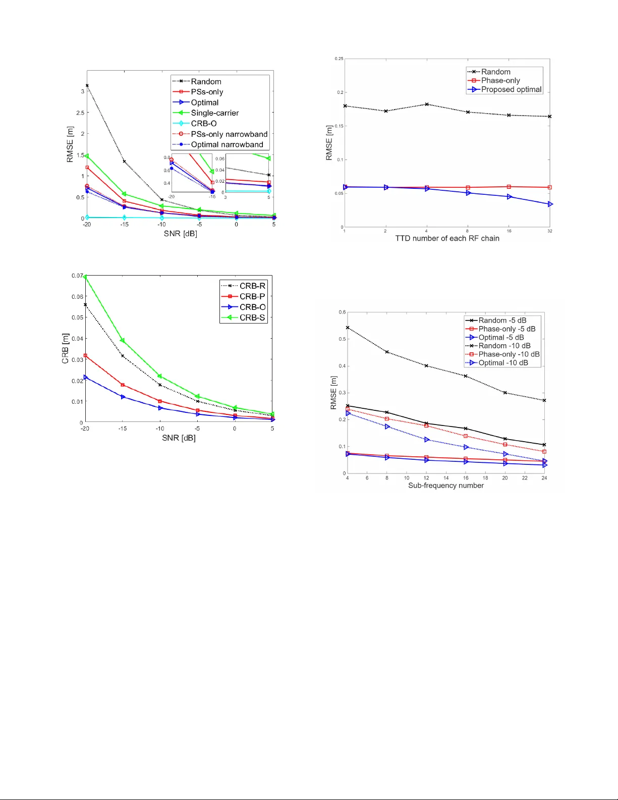
Near -Field W ideband Localization using TTD-Based T erahertz Extremely Lar ge-Scale Arrays Qianyu Y ang, Member , IEEE , Haiyang Zhang, Member , IEEE , Francesco Guidi, Member , IEEE , Anna Guerra, Member , IEEE , Davide Dardari, F ellow , IEEE , Baoyun W ang, Senior Member , IEEE , and Y onina C. Eldar , F ellow , IEEE Abstract —The syner gy between extremely large-scale antenna arrays and terahertz technology in sixth-generation networks estab- lishes a near -field wideband transmission envir onment, enabling the generation of highly focused beams. T o leverage this capability for multi-source localization, we propose a direct localization method based on the curvatur e-of-arrival of spherical wa vefronts f or estimating the positions of multiple near -field users from wideband signals. Furthermore, to over come the spatial-wideband effect, we introduce a hybrid analog/digital array architectur e with true-time- delayers (TTDs). W e derive a closed-form position err or bound to characterize the fundamental estimation performance and optimize the analog coefficients of array by maximizing the trace of the Fisher information matrix to minimize this bound. Furthermore, we extend this method to a sub-optimal iterative method that jointly optimizes beam f ocusing and localization, without requiring prior knowledge of the sour ce positions for array design. Simulation results show that the proposed array configuration design significantly enhances the performance of near -field wideband localization, while the presence of TTDs effectiv ely mitigates the localization performance degradation caused by spatial-wideband effects. I . I N T R O D U C T I O N In sixth generation (6G) networks, the integration of extremely large-scale antenna arrays (ELAAs) and the utilization of T erahertz (THz) bands are expected to notably enhance radio fre- quency (RF) positioning accurac y [ 1 ]. Specifically , THz wideband radio positioning is expected to undergo significant advancements and widespread adoption, as the wide bandwidth a vailable will result in high spatial resolution, and the feasibility of large antenna arrays enables unprecedented angular resolution [ 2 ]–[ 4 ]. The transition towards ELAAs and the incorporation of THz frequency bands entail more than just an increase in bandwidth and the ability to stack more antenna elements on a gi ven platform [ 5 ]–[ 7 ]. These advancements inv olve operating with fe wer RF chains than elements and integrating analog processing to a certain extent in 6G networks [ 8 ]–[ 10 ]. They also bring Q. Y ang is with the School of Information and Software Engineering, East China Jiaotong Univ ersity , Nanchang 330013, China (e-mail: 3763@ecjtu.edu.cn). B. W ang is with the School of Communication and Information Engineering, Nanjing University of Posts and T elecommunications, Nanjing, China (e-mail: bywang@njupt.edu.cn). H. Zhang is with the School of Communication and Information Engineering, Nanjing Uni versity of Posts and T elecommunications. He is also with the National Mobile Communications Research Laboratory , Southeast University , Nanjing 210096, China (e-mail: haiyang.zhang@njupt.edu.cn). F . Guidi is with the National Research Council of Italy , IEIIT , Bologna, Italy (e-mail: francesco.guidi@cnr.it). A. Guerra and D. Dardari are with the Department of Electrical, Electronic, and Information Engineering Guglielmo Marconi - DEI-CNIT , Uni versity of Bologna, Cesena, Italy (e-mail: { anna.guerra3,davide.dardari } @unibo.it). Y . C. Eldar is with the Faculty of Math and CS, W eizmann Institute of Science, Rehovot, Israel (e-mail: yonina.eldar@weizmann.ac.il). about substantial alterations in the electromagnetic characteristics of the wireless en vironment, transitioning from planar wa ve to spherical wa ve propagation, thereby signal transmission occurrs within the radiating near-field region [ 1 ], [ 11 ]. Hybrid architectures, which utilize fe wer RF chains than antenna elements, often employ phase shifter (PS) networks [ 12 ]–[ 14 ] to connect multiple antennas to less RF chains, forming arrays with high-dimensional analog processing and lo w-dimensional digital processing. Howe ver , in THz systems, the spatial-wideband effect leads to beam split, causing non-ov erlapping main lobes of the array gain corresponding to the lowest and highest subcarriers, resulting in a significant degradation of positioning estimation accuracy [ 15 ], [ 16 ]. Specifically , PSs are typically optimized for a single frequency (i.e., the central frequency), while in wideband systems, dif ferent frequencies across the band experience different phase shifts due to their v arying wav elengths. Since phase shifters do not account for these v ariations across frequencies, the direction of the main beam ”splits” or shifts off the intended target as the frequenc y moves away from the center . This shift creates an unintended offset in the beams direction, especially noticeable in systems with a large frequency range. While matrix projection techniques aim to alle viate this issue [ 17 ], their effecti veness is hampered by the frequency-independent nature of PSs [ 18 ]. T o address this challenge, true-time delayers (TTDs) can be integrated into arrays to enable frequency-dependent beamform- ing. Specifically , the time delay introduced by TTDs induces frequency-dependent phase shifts across dif ferent subcarriers, thereby enabling distinct beamforming patterns to be applied to each subcarrier signal with dif ferent frequency and ef fectively mitigating the beam squint ef fect. Moreover , to manage the high power consumption and hardware complexity of TTDs, mainstream TTD-based hybrid arrays typically incorporate a limited number of TTDs between the PSs and RF chains [ 19 ]– [ 22 ]. For instance, [ 19 ] analyzed the array gain loss resulting from the beam splitting ef fect in THz massi ve MIMO systems and addressed the issue through the incorporation of TTDs. Meanwhile, [ 20 ] extended TTD-based wideband beamforming to the near-field scenario. Based on the conv entional fully-connected TTD-based architecture, [ 21 ] considered practical maximum delay constraints of TTDs and proposed a hybrid serialparallel TTD configuration that relaxes the maximum delay requirements per TTD. Furthermore, [ 22 ] introduced a partially-connected TTD-based hybrid architecture aimed at improving energy effi- ciency and reducing the number of TTDs required. These studies demonstrate that these configurations can achiev e near-optimal 1 performance in terms of communication rates while minimizing po wer consumption. Nev ertheless, the utilization of TTD-based hybrid architectures for wideband localization in the radiating near-field has been relativ ely ov erlooked in existing literature. Differently from far-field localization scenarios [ 23 ], [ 24 ], in the radiating near-field, where wireless systems employing ELAAs at high frequency bands are expected to operate, the spherical shape of the wav efront becomes non-negligible [ 25 ]. Such wa vefronts introduce new degrees of freedom that can be le veraged to enhance wireless localization, enabling direct and precise localization [ 26 ]–[ 32 ]. This method in volves estimating positions, including distance and azimuth of users, directly from the curv ature of the spherical wav efront, known as the curv ature-of-arriv al (COA) based localization technique [ 33 ]–[ 35 ]. Recent studies in the realm of 6G ha ve considered COA-based localization, focusing on various aspects such as characterizing the Cramer-Rao bound (CRB) [ 33 ], exploring RIS-assisted config- urations [ 34 ], and tracking methods [ 35 ]. Additionally , [ 36 ], [ 37 ] inquired near-field localization with hybrid arrays, sho wcasing the design of analog coefficients in hybrid arrays for near-field local- ization can achie ve a form of beamfocusing. Similar findings were reported for integrated sensing and communications in [ 38 ], [ 39 ]. Most existing works of near-field wireless positioning focus on narrowband scenarios. Howe ver , with the advent of 6G technologies like ELAAs and THz technology systems, many applications operate in wideband near-field en vironments [ 22 ], which is far less studied compared to its narro wband counterparts. In particular, [ 40 ] inv estigated near-field processing for THz systems with a sparse transcei ver array , but impact of the beam split was ov erlooked. The work [ 41 ] employed a noise subspace correction approach to address the beam split ef fect, yet it fails to mitigate the array gain loss stemming from this phenomenon. This motiv ates exploring wideband near-field multi-user localization using a TTD-based hybrid array . In this work, we in vestigate RF positioning based on maximum likelihood (ML) estimation using wideband signals in the radiating near-field with a hybrid antenna array . T o mitigate the beam split ef fect inherent in wideband systems, we employ hybrid arrays incorporating TTD units. Furthermore, we optimize the analog coefficients (i.e., the phase of PSs and the delay of TTDs) to enhance localization performance. Based on a nov el problem formulation, we deri ve a closed-form expression for the CRB on ML position estimation. This deriv ation elucidates ho w the design of analog coefficients impro ves localization accurac y in wideband settings by maximizing the Fisher information matrix (FIM). Subsequently , we de velop an iterativ e algorithm utilizing alternating optimization to simultaneously achieve beam focusing and user localization. Our main contributions are summarized as follo ws: • TTD-Based Wideband CO A-Based Localization: W e present a COA-based wideband localization method, designed to achie ve simultaneous localization and beam focusing in the radiating near field with a TTDs-based hybrid array . • Fundamental Localization Limits Analysis: W e deriv e the CRB for the position estimates obtained via the proposed localization algorithm, which demonstrates the connection between the localization performance and the analog coef ficients design. Subsequently , we formulate an optimization problem for the design of analog coefficients to minimize the CRB, enhancing the effecti veness of the localization algorithm. • Beamfocusing Algorithm: W e employ an alternating op- timization approach to reframe the analog coefficients coupling optimization problem into two separate sub- problems: one concerning the PSs coefficients and the other the TTDs coefficients. These sub-problems are solved indi vidually based on assumed user positions, allowing us to iteratively con verge on an approximate solution to the original problem. Subsequently , we expand our design to include a sub-optimal iterativ e method that eliminates the need for prior knowledge of user positions. • Extensi ve Simulation Analysis: W e conduct a comprehen- siv e numerical analysis to showcase that the proposed solution notably boosts the performance of wideband near- field localization. The rest of the paper is or ganized as follows: Section II describes the considered wideband signal model and antenna architecture. Section III formulates CO A-based localization for a giv en beampattern, and analyzes its associated CRB. In Section IV , we formulate joint beamfocusing and localization as an optimization problem, based on which the proposed algorithm is deriv ed. Subsequently , Section V reports the numerical results. Finally Section VI provides concluding remarks. Notations : Scalar v ariables, vectors, and matrices are represented with lower letters, lower bold letters, and capital bold letters, respectively (e.g., x , x , and X , respecti vely). The term C N × N denotes a complex space of dimension N × N , the superscripts ( · ) T and ( · ) H denote the transpose and Hermitian transpose, respecti vely , | · | is the absolute value operator, ∥ · ∥ is the Frobenius norm, blkdiag ( X 1 , · · · , X N ) denotes a block diagonal matrix with diagonal blocks X 1 , · · · , X N , and [ x ] n denotes the n -th elements of v ector x . I I . S Y S T E M M O D E L In this section we present the considered wideband near-field localization system model. W e first formulate the corresponding receiv ed signal model in Section II-A , and then introduce the considered array architectures in Section II-B . A. Received Signal Model W e consider a multi-user localization scenario in which a base station receives pilot signals from K single-antenna users to esti- mate their locations. The base station comprises a uniform linear array (ULA) with N antenna elements separated by a distance ∆ . In the uplink transmission, all users share the pilot spectrum, transmitting M Orthogonal Frequency-Di vision Multiplexing (OFDM) subcarriers within a bandwidth B at central carrier frequency f c . Accordingly , the frequency of the m -th subcarrier with m ∈ 1 , · · · , M , defined as f m , is obtained from a uniform di vision of the frequency interv al [ f c − B / 2 , f c + B / 2] . When communication takes place in traditional bands (e.g., sub 6 GHz), it is possible to uniformly process each subcarrier based on f c . Ho wev er, in highly wideband (e.g., Thz) systems, the large bandwidth results in the beam splitting ef fect, and the frequency difference of each subcarrier cannot be ignored. 2 T o formulate the resulting signal model, let x m = [ x m, 1 , · · · , x m,n , · · · , x m,N ] T ∈ C N denote the receiv ed signal components of the m -th subcarrier at the base stations’ s array . Each source emits a standardized pilot signal with unit po wer . The signal receiv ed by the n -th antenna of the ULA at a specific discrete time instance can be expressed as: x m,n = K X k =1 x m,k,n + z m,n . (1) In ( 1 ), z m,n is the additiv e white Gaussian noise at the n -th antenna for the m -th pilot symbol which has variance σ 2 m , and x m,k,n is the receiv ed signal of the m -th subcarrier from the k -th user at the corresponding antenna. The latter can be expressed as x m,k,n = g m,k,n c k , (2) where c k is the data symbol corresponding to the k -th user , which satisfies E {| c k | 2 } = 1 , and g m,k,n = α m,k e − j v m,k,n represents the channel component, with α m,k and v m,k,n denoting the channel gain coefficient and the phase due to the distance traveled by the signal, respectiv ely . The gain is expressed as α m,k = c 4 π f m d k with d k indicating the distance between the array and the user 1 , and the phase is gi ven by v m,k,n ≜ 2 π f m d k,n c . (3) In ( 3 ) , d k,n is the distance between the corresponding antenna and the user , and c is the speed of light. Consequently , x m can be written as x m = K X k =1 g m,k c k + z m = G m c + z m , (4) where g m,k = [g m,k, 1 , · · · , g m,k,n , · · · , g m,k,N ] T ∈ C N × 1 and z m = [ z m, 1 , · · · , z m,n , · · · , z m,N ] T ∈ C N × 1 denote the channel vector and noise v ector, respecti vely . The matrix G m = [ g m, 1 , · · · , g m,K ] ∈ C N × K is the channel matrix, and c = [ c 1 , · · · , c K ] T ∈ C K × 1 denotes the symbol vector . B. Array Ar chitectur e The antenna array utilized by the base station is based on a hybrid architecture, being a widely adopted technique for realizing lar ge scale antennas at high frequencies in an affordable manner [ 10 ]. W e specifically consider TTD-based hybrid array configurations, in which large number of antenna elements is connected to a smaller number of RF chains through dedicated analog circuitry comprised of TTD units, as depicted in Fig. 1 . In this architecture, TTD-based preprocessing of the receiv ed signal achieves frequency-independent phase adjustment. This TTD-based hybrid array setup employs N d RF chains to connect to N antennas utilizing a restricted lev el of analog signal processing, each antenna connects to an RF chain via an individual PS and a shared TTD [ 22 ]. Specifically , the array is partitioned into several linear sub- arrays, each comprising N s elements arranged uniformly . Each linear sub-array is managed by a fully interconnected PS network 1 Here we neglect the near-field model of amplitudes, as abov e variation in channel gain between different antennas of the array is small enough [ 42 ]. with a TTD. Subsequently , the TTDs are divided into N d groups, each containing N t TTDs, with each group linked to an RF chain. Consequently , the array incorporates N t N s TTDs and N PSs, sat- isfying the condition N = N d N t N s . The signal of the m -th sub- carrier y m = [ y m, 1 , · · · , y m,i , · · · , y m,N d ] T ∈ C N d × 1 , which is processed in digital after analog combination, is thus given by y m = Q m x m , (5) where Q m is the analog combination matrix, which is determined jointly by the TTDs and PSs as Q m = T m A . (6) In ( 6 ), T m ∈ C N d × N d N t and A ∈ C N d N t × N represent the analog processing carried out by the TTDs and PSs, which are giv en by T m = blkdiag  e j 2 πf m t 1 , · · · , e j 2 πf m t N d  , (7) A = blkdiag ( a 1 , 1 , · · · , a i,l , · · · , a N d ,N t ) , (8) respecti vely . In ( 7 ) t i = [ t i, 1 , · · · , t i,N t ] ∈ C N t is the time delay vector of TTDs at the i -th RF chain, with t i,l ∈ [0 , t max ] , i ∈ { 1 , · · · , N d } , l ∈ { 1 , · · · , N t } , here t max being the maximum delay of each TTD. In ( 8 ) , a i,l ∈ C N s is the PS coefficient vector connect to the l -th TTD at the i -th RF chain, its internal element a n denotes the coefficient of the PS corresponding to the n -th antenna with n ∈ N i,l = { (( i − 1) N t + l − 1) N s + 1 , · · · , (( i − 1) N t + l ) N s } , which is frequency independent and gi ven by a n ∈ F ≜  e j ϕ n | ϕ n ∈ [0 , 2 π ]  . (9) Hence, the entries of the digital input ( 5 ) can be expressed as y m,i = N t X l =1 e j 2 πf m t i,l X n ∈N i,l a n x m,n . (10) Our objecti ve is to estimate user positions based on receiv ed wideband signal observations { y m } M m =1 . As evident from ( 5 ) and ( 10 ), the considered array architecture facilitates distinct analog combinations for each received signal y m . Therefore, by adjusting the combinations constrained by ( 7 ) and ( 8 ), the received signal will be subjected to frequency dependent modulation to av oid beam splitting. I I I . L O C A L I Z A T I O N W I T H F I X E D A N A L O G C O M B I N A T I O N The array architecture modeling in ( 10 ) indicates that one can af fect the signal processed in digital (and used for localization) by manipulating the analog configuration Q m , represented by T m and A . T o understand how the setting of these analog combining parameters af fect the ability to localize multiple users based on wideband transmission, we start by studying localization for a fixed analog combiner and analyze the associated CRB of estimation rusult. T o that aim, we first characterize a suitable localization algorithm based on the maximum likelihood rule before the CRB analysis. A. Maximum Likelihood Localization 1) Localization Setting: The utilization of the radiating near - field in communication can be leveraged to enhance localization 3 Fig. 1. System model diagram. Left diagram: the array architectures; Right diagram: the localization scenario. through the CO A estimation of the impinging signal at dif ferent antennas. The localization scenario under consideration, depicted in Fig. 1 , establishes a reference point (an antenna) u 0 situated at (0 , 0) within the recei ving array . The ULA is oriented along the Y -axis, with the k -th user positioned at (x k , y k ) , a distance of d k , and an azimuth angle θ k relativ e to the source (refer to Fig. 1 ). Moreov er , the n -th antenna of the array is positioned at (0 , r n ) with respect to the array’ s reference point, where r n = ( N − 1)∆ . The specific geometric relationships between coordinates and reference positions can be described as: x k = d k cos θ k , y k = d k sin θ k . (11) According to the triangular relationship, the distance of the k th user from the n th antenna can be e xpressed as [ 35 ] d k,n ( d k , θ k ) = q r 2 n + d 2 k − 2 r n d k cos θ k . (12) 2) Maximum Likelihood F ormulation: The formulation ( 12 ) establishes the intricate link between the user’ s location and the phase distribution, preserving the nonlinearity within the aforementioned output. Hence, one viable approach for user position estimation in volves the computation of the maximum likelihood estimation (MLE). By consolidating the received signals across M sub-frequencies, we ha ve y =  y T 1 , · · · , y T M  T , which we express as y = QG ˆ c + Q z , (13) where ˆ c = l M ⊗ c ∈ C M K × 1 , z =  z T 1 , · · · , z T M  T , Q = blkdiag ( Q 1 , · · · , Q M ) , G = blkdiag ( G 1 , · · · , G M ) . According to ( 7 ) and ( 8 ), we hav e Q m Q T m = N t N s I N d , ∀ m . W e define the unknown parameters vector to be estimated from ( 13 ) as η = [ d , θ ] ∈ C 2 K , with d = [ d 1 , · · · , d K ] and θ = [ θ 1 , · · · , θ K ] refer to the possible user positions set in polar coordinates, respectiv ely . The position MLE is giv en by ˆ η = arg max η log p ( y ; η , Q ) , (14) where log p ( y ; η , Q ) is the log-likelihood function of y . The MLE process is based on an observation time window consisting of L samples. The l -th sample is denoted as y ( l ) for l = 1 , · · · , L . Gi ven ( 13 ), once a sufficient quantity of receiving samples is obtained, the log-likelihood function of y can be articulated as [ 43 ] log p ( y ; η , Q ) = log p ( y 1 , · · · , y M ; η , Q ) ∝ L X l =1 M X m =1 ∥P [ S m ( η , Q )] y m ( l ) ∥ 2 ∝ M X m =1 tr [ P [ S m ( η , Q )] R m ] , (15) where R m is the empirical a verage of y m y H m ov er the observed time window , and P denotes the projection operator , which, when applied to a matrix X , is gi ven by P [ X ] = X  X H X  − 1 X H . Projection in ( 15 ) is applied to S m ( η , Q ) = Q m S d m ( η ) , and S d m ( η ) =  s d m, 1 ( η 1 ) , · · · , s d m,K ( η K )  ∈ C N × M is the steering matrix of the array with s d m,k ( η k ) = α m,k h e − j v m,k, 1 ( η k ) , · · · , e − j v m,k,N ( η k ) i T , (16) where η k = [ d k , θ k ] , and v m,i,l ( η k ) is obtained from ( 3 ) and ( 12 ) thus determined by η k . 3) MLE Computation via Alternating Pr ojection: Problem ( 15 ) can be solved by the alternating projection (AP) method to av oid the complexity of the multi-dimensional maximization prob- lem [ 37 ]. Specifically , we define the vector η − k = [ d − k , θ − k ] ∈ C 2 K − 2 , where d − k = [ d 1 , · · · , d k − 1 , d k +1 , · · · , d K ] and θ − k = [ θ 1 , · · · , θ k − 1 , θ k +1 , · · · , θ K ] , then the projection operator P [ S m ( η , Q )] can be rewritten as P [ S m ( η , Q )] = P  S m  η − k , Q  + P [ s m ( η k , Q )] , (17) 4 where S m  η − k , Q  ∈ C N d × K − 1 is the steering matrix based on η − k and Q , and s m ( η k , Q ) is giv en by s m ( η k , Q ) =  I N d − P  S  η − k , Q  Q m s d m,k ( η k ) , (18) which denotes the residual of Q m s d m,k when projected on S m  η − k , Q  From ( 17 ), for a giv en analog configuration Q , once η − k has been fixed, P [ S m ( η , Q )] becomes solely reliant on η k . Consequently , the maximization of ( 15 ) can be addressed alternating iterativ ely with each iteration in volving the maximization concerning a single parameter η k while keeping all other parameters constant. Thus, by substituting ( 17 ) into ( 15 ) , the problem posed in ( 14 ) can be streamlined into solving M sub-problems, where the m -th sub-problem is formulated as: η k = arg max η k log p ( y ; η k , Q ) ∝ M X m =1 tr [ P [ s m ( η k , Q )] R m ] (19) One can calculate ( 19 ) when Q is held constant, with the detailed process summarized as Algorithm 1 . The initial estimation begins with a single-user scenario to determine the position of the first user . Subsequently , the algorithm fixes the existing estimates and progressively incorporates additional users until reaching the final estimation. This incremental approach aids in refining the localization process step by step. W e note that the proposed Algorithm 1 is also applicable to narro wband system. In narrowband system case, all subcarriers would be tuned by a unified phase shift from PSs without TTDs, that Q would be gi ven by Q = blkdiag ( Q 0 , · · · , Q 0 ) , where Q 0 is obtained from ( 6 ) with t max = 0 . Algorithm 1 AP-based wideband near -field localization. Initialize: Set t = 1 ; The maximal number of iteration K t ; η ∈ R 2 K , and P [ S m ( η , Q )] = 0 , ∀ m . For k = 1 : K 1: For all m , calculate: s m ( η k , Q ) = ( I N d − P [ S m ( η , Q )]) Q m s d m,k ( η k ) . 2: Obtain η 0 k by solving ( 19 ) with calculated s m ( η k , Q ) . 3: P [ S m ( η , Q )] = P [ S m ( η , Q )] + P [ s m ( η k , Q )] . 4: Initialize position set: [ η ] k = [ η 0 k ] 1 , [ η ] K + k = [ η 0 k ] 2 . End While t ≤ K t do For k = 1 : K 5: Obtain P [ s m ( η k , Q )] from s m ( η k , Q ) as ( 18 ), ∀ m . 6: Obtain η t k by solving ( 19 ) with calculated s m ( η k , Q ) . 7: Update position set: [ η ] k = [ η t k ] 1 , [ η ] K + k = [ η t k ] 2 . 8: Update P [ S m ( η , Q )] = P [ S m ( η , Q )] + P [ s m ( η k , Q )] . End 9: t = t + 1 . End while Output: The estimated unkno wn parameters η . The computation of Algorithm 1 requires a given Q . Therefore, the fact that the accuracy of this estimate depends on Q allows us to use the above MLE as guidelines for the analog design along with the localization task. B. Cramer-Rao Bound Analysis The CRB serv es as a fundamental lo wer limit on the variance of any unbiased estimator [ 44 ]. The CRB expression deri ved provides valuable insights into ho w system parameters and configurations, such as the analog combination, influence the performance of position estimation. For the likelihood model in ( 15 ), the array output y can be regarded as a distribution with the mean vector µ and covariance matrix Ξ = blkdiag ( σ 2 1 N t N s I M N d , · · · , σ 2 M N t N s I M N d ) , where µ = QS d ( η , Q ) ˆ c , (20) and S d ( η , Q ) = blkdiag  S d 1 ( η , Q ) , · · · , S d M ( η , Q )  . Let F denotes the Fisher information matrix (FIM) for estimating parameter η from the data. The elements of the FIM are given by [ 45 ] [ F ] i,j = 2 R  ∂ µ H ∂ [ η ] i Ξ − 1 ∂ µ ∂ [ η ] j  + tr  Ξ − 1 ∂ Ξ ∂ [ η ] i Ξ − 1 ∂ Ξ ∂ [ η ] j  = 2 R  ∂ µ H ∂ [ η ] i Ξ − 1 ∂ µ ∂ [ η ] j  , (21) where [ η ] i denotes the i -th element of η . According to ( 20 ) and the definition of Q , we hav e the first-order deriv ativ e ∂ µ ∂ d = Q ∂ S d ( η , Q ) ∂ d ˆ c =  CD T 1 Q T 1 , · · · , CD T M Q T M  T , (22) ∂ µ ∂ θ = Q ∂ S d ( η , Q ) ∂ θ ˆ c =  CB T 1 Q T 1 , · · · , CB T M Q T M  T . (23) Here C = diag ( c ) , D m and B m are respectively defined as D m = " ∂ s d m, 1 ( η 1 ) ∂ d 1 , · · · , ∂ s d m,K ( η K ) ∂ d K # ∈ C N × K , (24) B m = " ∂ s d m, 1 ( η 1 ) ∂ θ 1 , · · · , ∂ s d m,K ( η K ) ∂ θ K # ∈ C N × K . (25) The elements of the matrix in ( 24 ) and ( 25 ) are giv en by [ D m ] n,k = ∂ s d m,k,n ∂ d k = − e − j v m,k,n  c 4 π f m d 2 k + j ( d k − r n cos θ k ) 2 d k d k,n  , (26) [ B m ] n,k = ∂ s d m,k,n ∂ θ k = − e − j v m,k,n j r n sin θ k 2 d k,n . (27) Then, according to the division of η , the FIM can be represented as F =  F dd F d θ F θ d F θθ  , (28) 5 where each block matrix in ( 28 ) can be calculated separately as F dd = 2 R  ∂ µ H ∂ d T Ξ − 1 ∂ µ ∂ d  = 2 N t N s M X m =1 1 σ 2 m R  C H D H m Q H m Q m D m C  , (29) F d θ = 2 R  ∂ µ H ∂ d T Ξ − 1 ∂ µ ∂ θ  = 2 N t N s M X m =1 1 σ 2 m R  C H D H m Q H m Q m B m C  , (30) F θ d = 2 R  ∂ µ H ∂ θ T Ξ − 1 ∂ µ ∂ d  = 2 N t N s M X m =1 1 σ 2 m R  C H B H m Q H m Q m D m C  , (31) F θθ = 2 R  ∂ µ H ∂ θ T Ξ − 1 ∂ µ ∂ θ  = 2 N t N s M X m =1 1 σ 2 m R  C H B H m Q H m Q m B m C  , (32) T o con vert the estimation results from polar coordinates to Euclidean coordinates, we define the position parameter vector p = [x 1 , · · · , x K , y 1 , · · · , y K ] . Its corresponding FIM defined as F E is obtained by using the chain rule: F E = JFJ T , (33) with J = ∂ η ∂ p T ∈ C 2 K × 2 K denoting the Jacobian matrix, which can be computed based on the relationship specified in ( 11 ). The CRB is given by the in verse of F E , formulated as: CRB = q tr  F − 1 E  . (34) C. Discussion Once Q is given, the position error bound (PEB) of the estimated position p can be given by the CRB expression in ( 34 ) . This relationship motiv ates further in vestigation into ho w analog design influences localization performance. Although ( 34 ) provides a closed-form expression for the PEB, it does not explicitly reveal the dependence of localization accuracy on analog design. Instead, as ( 33 ) and ( 34 ) , the structure of the FIMs in ( 29 ) - ( 32 ) explicitly demonstrates which factors affect the localization performance. Specifically , we will explore the factors that af fect maximizing the trace of the FIMs, in order to achieve the minimization of CRB. Firstly , each block matrix of the FIM can be decomposed into a superposition of M submatrices corresponding to different subcarrier components. This decomposition implies that wideband transmission with richer spectral resources can enhance localization accuracy by reducing the CRB. Specifically , a larger number of subcarriers increases the o verall FIM, thereby lo wering the CRB as indicated by ( 34 ). Furthermore, this formulation establishes an intermediate relationship between Q and the localization CRB: given the user positions and frequency bands, the FIM is primarily determined by 2 Q . Further analysis reveals that the optimal analog design for maximizing different subcarrier components of FIMs varies, highlighting the significance of our work. By incorporating TTD units into the analog beamforming structure, frequency dependent phase control can be achie ved, enabling more precise optimization of each FIMs component across subcarriers. This leads to a lower CRB and improved localization accuracy . Therefore, the number of TTDs is a critical factor influencing the localization performance of the proposed wideband near-field localization scheme, as an increase in the former will be beneficial for more flexible frequency independent phase control. I V . A NA L O G C O M B I N A T I O N C O E FFI C I E N T D E S I G N While the localization scenario considered in the pre vious section focused on fixed analog combining (which dictates the beampattern of the ELAA), we next utilize its formulation to jointly localize and analog combining design generated by the TTD-based ELAA. W e thus formulate the optimization problem of analog coefficient design in Section IV -A . In Section IV -B , we optimize the phase of PSs for a fixed time delay configuration, then optimizing the time delay of TTDs for a fix ed PSs configuration. Finally , in Section IV -C , we extend these designs to also carry out localization, via an iterative algorithm for joint optimization position estimation and analog coefficient design. A. Pr oblem F ormulation According to ( 6 ), the design of PSs and TTDs contribute to effecti ve localization le veraging the hybrid array setup, where PSs are frequency independent while TTDs are frequency dependent. By optimizing the configurations of PSs and TTDs, the localization process can be enhanced, ultimately leading to improved accuracy and reliability in position estimation. As discussed in Section III-C , we design Q to maximize the average of the trace of FIM 3 , which is expressed as max { Q m } M m =1 tr[ F ] s.t. ( 9 ) , ( 7 ) , ( 8 ) , t i,l ∈ [0 , t max ] . (35) According to ( 28 ) - ( 32 ) , by substituting the definition of Q and removing the irrelev ant v ariable, problem ( 35 ) can be re written as max { T m } M m =1 , A M X m =1 tr  T m A U m U H m A H T H m  s.t. ( 9 ) , ( 7 ) , ( 8 ) , t i,l ∈ [0 , t max ] . (36) Where U m = D m + B m . Given the structural constraints outlined in ( 7 ) and ( 8 ) , Problem ( 36 ) is non-con ve x, primarily 2 Although the FIM also depends on the symbol matrix C as shown in ( 29 ) - ( 32 ) , this work assumes no interaction between users and the base station, and thus treats pilot symbols as random v ariables without optimizing their design. Howe ver , in scenarios inv olving user-base station coordination, pilot optimization could further impro ve localization performance. 3 The randomness inherent in pilot symbols results in variations in the FIM obtained from each sampling instance. Consequently , it is necessary to compute the statistical average to mitigate the effects of this v ariability . 6 due to the coupled nature of the optimization variables, i.e., T m and A . T o address this challenge, an alternate optimization strategy is employed to disentangle T m and A . This iterativ e alternate approach continues until con vergence is achieved, facilitating the optimization process in a computationally feasible manner to approximate the optimal solution. B. Alternating Optimization for TTDs and PSs 1) Phase design for given time delay: For given T m , the constrains on t i,l and structure constraint ( 7 ) in problem ( 36 ) can be removed. Define u m,k as the k -th column of U m and a = vec ( A ) ∈ C N d N × 1 . Then T m Au m,k = ( u m,k ) T ⊗ T m a . Define W m,k = ( u m,k ) T ⊗ T m . W e can then remov e the structure constraint ( 8 ) in ( 36 ) and rewrite the problem as max a a H M X m =1 K X k =1 W H m,k W m,k ! a s.t. ( 9 ) . (37) Gi ven that the zero elements of a does not impact the objecti ve function of ( 37 ), ( 37 ) can be simplified as max ˜ a ˜ a H M X m =1 K X k =1 ˜ W H m,k ˜ W m,k ! ˜ a s.t. ( 9 ) . (38) where ˜ a = [ a 1 , · · · , a N ] T ∈ C N is the modified version of a obtained by removing all the zero elements of a , and ˜ W m,k is the modified version of W m,k by removing the elements having the same index as the zero elements of a . According to the constraint ( 9 ) , solving ( 38 ) can be viewed as a search process for R with the searching space is a product of N complex circles, which is a Riemannian submanifold of C N . Consequently , addressing ( 38 ) can be accomplished using the Riemannian conjugate gradient (RCG) algorithm. Specifically , the solution to ( 38 ) is iterati vely updated according to [ ˜ a ( p +1) ] n = [ ˜ a ( p ) + ϵ ( p ) ξ ( p ) ] n | [ ˜ a ( p ) + ϵ ( p ) ξ ( p ) ] n | , ∀ n. (39) Here, [ ˜ a ( p +1) ] n represents the updated point derived from the current point [ ˜ a ( p ) ] n , with p indicating the iteration count. The solution utilizing the RCG method can be seen as an enhancement o ver the projection-based approach. ϵ ( p ) denotes the Armijo step size [ 25 ] in the p -th iteration, while ξ ( p ) signifies the search direction at the point ˜ a ( p ) , lying within the tangent space of the complex circle manifold at that specific point. This direction is giv en by w ξ ( p ) = − grad g ( ˜ a ) + ζ ( p )  ξ ( p − 1) − Re  ξ ( p − 1) ◦ ˜ a ( p ) †  ◦ ˜ a ( p )  , (40) where † and ◦ signify conjugation and the Hadamard product respectiv ely , ζ ( p ) is selected as the Polak-Ribiere parameter [ 25 ]. grad g ( ˜ a ) represents the Riemannian gradient of g ( ˜ a ) , computed as the orthogonal projection of the Euclidean gradient of g ( ˜ a ) , given by grad g ( ˜ a ) = ∇ g ( ˜ a ) − Re  ∇ g ( ˜ a ) ◦ ˜ a ( p ) †  ◦ ˜ a ( p ) , (41) where ∇ g ( ˜ a ) is the Euclidean gradient of g ( ˜ a ) , which is defined from ( 38 ) as ∇ g ( ˜ a ) = 2 M X m =1 K X k =1 ˜ W H m,k ˜ W m,k ! ˜ a . (42) W ith the giv en time delay setting of TTDs, we can compute { a n } N n =1 iterativ ely with ( 39 ) to ( 42 ), then we consider to determine the time delay with a giv en phase of PSs. 2) T ime Delay Design for Given Phase: For given A , ( 36 ) reduces to max { T m } M m =1 M X m =1 tr  T m A U m U H m A H T H m  s.t. ( 7 ) , t i,l ∈ [0 , t max ] , ∀ i, l . (43) W e define v m = v ec ( T m ) and Z m,k = ( Au m,k ) T ⊗ I N d and rewrite ( 43 ) as max ˜ v m M X m =1 ˜ v H m K X k =1 ˜ Z H m,k ˜ Z m,k ! ˜ v m s.t. ˜ v m =  e − j 2 πf m t 1 , · · · , e − j 2 πf m t N d  T , t i,l ∈ [0 , t max ] , ∀ i, l . (44) Here ˜ v m is the modified version of v m , and ˜ Z m,k is the modified version of Z m,k by removing the elements having the same index as the zero elements of v m . Problem ( 44 ) can be characterized as N d N t single-v ariable optimization problem concerning t i,l . Although deriving a closed-form solution for ( 44 ) is complex, the problem can be effecti vely addressed using numerical techniques like iterative one-dimensional search methods for practical computation. Specifically , define a searching set S = { 0 , t max /Q, 2 t max /Q, · · · , t max } , where Q is the sample number . In each iteration, each t i,l is updated by one-dimensional searching in S . C. Alternating Localization and Array Coefficient Design The analog design method pre viously discussed relies on location information that may not be readily accessible in practical scenarios. Nonetheless, drawing inspiration from [ 37 ], an ef ficient alternating optimization approach can be employed for joint analog domain design and localization. Specifically , [ 46 ] re veals that even when the focus position at the recei ving array de viates from the actual source position, improvements in the estimated results are observed. This enhancement persists despite discrepancies between the focus position and the user’ s true location, with the focus gain being present but attenuated. This suggests that once an initial estimation of the source location is acquired, iterativ e refinement towards the genuine source position is achiev able by updating the focus position. Simultaneously , the adjustment of Q m can be synchronized with the iterations in the AP algorithm. In essence, an alternating algorithm can be devised by inte grating the update of Q m into Algorithm 1 , which is summarized as Algorithm 2 . In Algorithm 2 , we utilize the recei ving vector deri ved from random coefficient responses to initialize the position estimation. Subsequently , we update the coef ficients of Q m based on the outcomes of the preceding position estimation to obtain new 7 Algorithm 2 Alternating localization and beamfocusing Initialize: Initialize the matrix { Q 1 m } M m =1 by the definition with random PSs setting A 1 and TTDs setting T 1 m which satisfies t i,l ∈ [0 , t max ] ; t = 1 ; Iterations limit K t . Obtain the initial position estimation as ( d 1 , θ 1 ) by Algorithm 1 (Steps 1-4). While t ≤ K t do For m = 1 : M 1: Estimate ( d t k , θ t k )) by maximizing ( 19 ) with gi ven Q t m . 2: Update position set: [ d ] k = d i k . End 3: Update A t via solving ( 37 ) with T m = T t m , ∀ m . 4: Update T t m via solving ( 43 ) with A = A t . 5: Update receiv e vector y t +1 from Q t +1 m by ( 13 ). 6: t = t + 1 End while Output: The position estimation ( d , θ ) = ( d K t , θ K t ) . observ ations. Different from the alternating algorithm in [ 37 ], in this paper the coefficient update is targeted at the wideband muti carrier scenarios, which require setting analog coef ficients for multiple subcarriers separately , and the relev ant design methods hav e been discussed in Section IV -B . This iterativ e procedure, repeated at each recei ving time slot, enables a step-by-step con- ver gence of the estimated result to wards the true source location. V . N U M E R I C A L E V A L U A T I O N S A. Simulation P ar ameters In this section, we provide numerical results to demonstrate the efficienc y of proposed localization algorithm and analog coef ficients design scheme. In our experiments, the recei ver array is set at configured as line array lying on the Y -axis with the array’ s reference position situated at (0 , 0) m, to positioning two users in X-Y plane, i.e., K = 2 . In this case, the position of two users is set as (8 m , π / 3) and (8 m , π / 4) in polar coordinates, respectiv ely . For conv enience, the noise variance σ 2 m is set to adjust SNR of each sub-carrier at antennas as a unified value, i.e., SNR = 10 log ( ∥ x m ∥ 2 / ( N σ 2 m )) , ∀ m . Furthermore, the other basic simulation parameters are gi ven in T able I , which is exploited throughout our simulations unless otherwise specified. The numerical indicators of localization performance are represented by the root mean square error (RMSE), calculated as RMSE = 1 K K X k =1 v u u t 1 N c N c X n c =1 e 2 k,n c , (45) where N c is the number of Monte Carlo iterations, e 2 k,n c = |  x k , y k  −  ˆ x ( n c ) k , ˆ y ( n c ) k  | 2 is the squared localization error (i.e., the distortion) of the k -th user ,  ˆ x ( n c ) k , ˆ y ( n c ) k  are the estimated coordinates at the n c -th Monte Carlo simulation. B. Numerical Results W e first demonstrate that the design of Q realizes a form of beam focusing, for this purpose, a heatmap is provided in Fig. 2 . Specifically , we consider a 20 × 20 , m 2 area with a resolution of 0 . 1 meters, where the antenna array is positioned at the origin. One user traverses all grid points and stays at each grid point for a positioning cycle to transmit pilot signals, T ABLE I E X P E R I M EN T P A R A M E T ER S Parameter V alue Central frequency f c = 300 GHz Bandwidth B = 30 GHz Subcarrier number M = 12 Sample number L = 256 Array antenna number N = 256 RF chain number N d = 8 TTD number per RF chain N t = 16 Antenna spacing ∆ = 5 × 10 − 4 m The maximum time delay t max = 5 ns Near-field distance d F = 32 . 5 m Fig. 2. The heatmap for the CRB on user position estimate by varying user positions, SNR is fixed as -10 dB. The magenta square denotes the array position. The red point is the predetermined position that analog design focuses on. while Q is designed to focus on the predetermined focal point as sho wn in Fig. 2 (i.e., Q is deri ved by solving problem ( 36 ) based on the FIMs corresponding to the fixed focal point). The array then localizes the user using the actual recei ved pilot signal with this fixed Q in each positioning cycle. As illustrated in Fig. 2 , the CRB for localization estimation is significantly reduced only when the user’ s true position is near the focal point of Q . This observ ation confirms the relationship between the proposed simulated beamforming design and the actual user position, thereby validating our claim that Q realizes a form of beam focusing in near field wideband localization. Then, to demonstrate the ef fectiv eness of the proposed localization algorithm, we provide one localization track map in the Monte Carlo simulation, as sho wn in Fig. 3 . In Algorithm 1 , localization is performed under a given Q , though this setup is not realistic in practice since the true user position is unknown, we assume that Q is perfectly designed to ensure a fair comparison with Algorithm 2 . By contrast, Algorithm 2 alternates between localization and Q design in an iterative manner . As observ ed, the estimated position trajectories of both algorithms gradually con verge from the initial estimate tow ard 8 Fig. 3. Position estimations track map for each iteration of Algorithm 1 and Algorithm 2 with SNR SNR = − 10 dB. Fig. 4. Contrast of the number of iterations required for conver gence via multiple contrast schemes with SNR = − 5 dB. the true user position as iterations proceed. Moreov er, it is worth noting that Algorithm 1 achiev es a more accurate initial position estimate compared to Algorithm 2 and con ver ges faster to the true position. This clearly highlights the impact of Q design on the overall localization performance. T o ev aluate the ef ficacy of the analog coef ficient design in the joint localization and beamfocusing algorithm, we initially explored the conv ergence behavior of Algorithm 2 , as illustrated in Fig. 4 . Here, the curve “ Alternating” refers to localization using the proposed Algorithm 2 with a random analog coefficient set as initial. For comparati ve analysis, we established three contrasting schemes with different initial error as 0 m, 0.5 m and 1 m. Specifically , in abov e contrast schemes, we still localization with Algorithm 2 , but assume that we have an indistinct pre knowledge of users locations, where the location error is a Gaussian-distributed random variable centered on the corresponding setting standard de viation, the initial analog coef ficient Q 1 m in Algorithm 2 is obtained by solving ( 37 ) and ( 43 ) with such initial locations. The extreme schemes are also provided, in v olve localization via Algorithm 1 with predetermined analog setting. In such schemes, “Random” indicates that A and T m are randomly set within specific constraints, while “Optimal” signifies that A and T m are iterati vely optimized by solving ( 37 ) and ( 43 ) with the perfect knowledge of users locations. In Fig. 4 , it is e vident from the results that the RMSE of the proposed alternate scheme gradually con ver ges from the lev el of the random scheme tow ards close to that of the optimal scheme, while the deviation of the con ver gence result depends on the initial error . Once the initial error is small enough, e.g., 0.5 m, it can achiev e the almost same performance as the optimal scheme which has the perfect knowledge of users locations. Although the alternate scheme generally necessitates more iterations for con ver gence compared to the optimal scheme, this is attributed not only to the initial position estimation b ut also to the additional updates for the analog design. Nonetheless, the iteration process for analog design proves to be efficient, by iterativ ely analog coef ficient design through Algorithm 2 , the localization accuracy has been improv ed from decimeter lev el to centimeter le vel. W e illustrate the effecti veness of the analog design scheme we proposed in Fig. 5 , displaying the RMSE of location estimation across various schemes under v arying SNRs. As pre viously discussed, the analog design scheme attains optimal performance when the position information is known. Therefore, we utilize the aforementioned optimal scheme as a benchmark for performance comparison and calculate the CRB under this optimal scenario denoted as “CRB-O”. T o showcase the performance enhancement deriv ed from the analog design and further highlight the performance gains resulting from the incorporation of a time delay de vice, we include the random scheme and the PSs-only scheme for comparison, above analog coefficients of schemes are design randomly , and derived by solving ( 36 ) with t max = 0 , serving as an additional reference point in the analysis, respectively . Additional, the single-carrier scheme is also pro vided to show the performance improvement from the multi-carriers introduction, where the single-carrier scheme is obtained from [ 37 ] by set M = 1 . Finally , to ev aluate the impact of the bandwidth to optimal scheme and phase-only scheme, we consider a narro wband case, i.e., “Optimal 2” and “Phase-only 2”, in such case, the the bandwidth is set as 300 MHz. In Fig. 5(a) , it is evident that the random scheme exhibits the highest RMSE compared to the other schemes in low SNR scenarios. Through the analog design achiev ed by solving ( 36 ) , a substantial enhancement in RMSE is observed. Besides, it can be seen that the PSs-only scheme would close to the optimal scheme in the narrowband case, since the beam split effect could be ignored in such case. Then in the wideband case, scenarios characterized by high SNRs, the proposed optimal localization scheme closely approaches the performance le vel of the CRB in comparison to the PSs-only scheme. While in low SNR en vironments, the former demonstrates around 40% of the performance enhancement achieved by the latter , it indicates the necessity of the introduction of TTDs for the wideband system. An intriguing observ ation in the single-carrier scheme is that 9 (a) RMSE versus dif ferent SNR. (b) CRB versus dif ferent SNR. Fig. 5. RMSE contrast of multiple contrast schemes under dif ferent SNR with array setting. (a) RMSE-SNR; (b) CRB-SNR while it exhibited the worest performance in high SNR scenarios, at lo w SNR lev els, its focus obtained through analog design nearly matched the performance of the PSs-only scheme. This futher indicates that the PSs network did not fully exploit the benefits of multi-carrier systems in wideband scenarios, underscoring the importance of incorporating TTDs in multi-carrier settings. T o elucidate the outcomes depicted in Fig. 5(a) , we present the CRB results from v arious schemes in Fig. 5(b) . Here, “CRB-R”, “CRB-P” and “CRB-S” are computed using ( 34 ) with analog design deri ved from the random scheme, the phase-only scheme and the single-carrier scheme, respectiv ely , under the bandwidth B 1 . The comparison of these CRB values mirrors the trends observed in the RMSE performance of their corresponding schemes, suggesting that the performance enhancement exhibited by the proposed scheme stems from its optimization of the CRB. In Fig. 6 , we observe the influence of the number of TTDs connected to each RF chain, denoted as N t , on the localization ef ficiency . T o ensure a fair comparison, we adjust the number of PSs connected to each TTD, denoted as N s , in accordance with the v ariation of N t to maintain the condition N = N d N t N s as specified in T abel I , that the upper limit of N t is N t = N / N d Fig. 6. RMSE contrast of multiple contrast schemes under different TTDs number of each RF chain with SNR = − 5 dB. Fig. 7. RMSE contrast of multiple contrast schemes under different subcarrier number with SNR = − 5 or -10 dB. with N s = 1 . The proposed optimal scheme demonstrates improv ed performance with increasing N t . This enhancement is attributed to the increased processing flexibility across multiple sub-carriers facilitated by the addition of more TTDs, thereby decelerate the beam splitting ef fect. In contrast, the performance of the random scheme and the phase-only scheme remains unaffected by changes in N t . Howe ver , this performance enhancement is not as pronounced when N t is less than the number of sub-carriers M . In such instances, the performance of the proposed optimal scheme tends to approach that of the phase-only scheme. Con versely , when the number of TTDs is maximized (i.e., one TTD per antenna), the localization performance exhibits the most substantial improvement. Howe ver , deploying a dedicated TTD for each antenna in an ELAA system may be impractical due to prohibiti ve cost considerations. T o further elucidate the impact of the relationship between the number of sub-carriers and the number of TTDs connected to 10 each RF chain on the performance of the proposed localization scheme, we present Fig. 7 showcasing the RMSE v ariations across dif ferent sub-carrier numbers. The results re veal that the performance of all schemes improves as the number of sub- carriers increases. This improvement can be attributed to the av ailability of more receiv ed information, a concept supported by the definitions of the FIMs deri ved in ( 29 ) - ( 32 ) . Furthermore, it is e vident that in scenarios with a small number of sub-carriers, the phase-only scheme closely matches the performance of the proposed optimal scheme. Ho wev er , as the number of sub-carriers grows, a performance gap emerges between the two schemes, particularly when the number of sub-carriers exceeds N t . This observ ation underscores that the primary adv antage of integrating TTDs lies in resolving the limitation of PSs network in accurately processing multiple sub-carrier signals due to their frequency independence. The ef fectiv eness of TTDs in managing multiple sub-carriers is contingent upon their quantity . A substantial performance enhancement necessitates a greater number of TTDs connected to each RF chain than the number of sub-carriers. V I . C O N C L U S I O N S In this work, our focus delved into wideband near-field multi-user localization utilizing a TTDs-based hybrid array . Initially , we elucidated the models pertaining to radiating near- field position estimation systems within the specified antenna architecture. Subsequently , we derived the CRB for the proposed estimation systems, and accordingly delineated the optimization strategy for the adjustable coefficients of the hybrid array to enhance position estimation accuracy , and introduced an ef ficient algorithm for simultaneous position estimation and adjustable coefficients design. The numerical outcomes underscored that the meticulous design of analog coefficients within the hybrid array wielded a substantial impact on enhancing near -field multi- source localization performance. Furthermore, the incorporation of TTDs was observed to improve the processing capabilities of the array , particularly in scenarios in volving multi-carrier signals. R E F E R E N C E S [1] H. Zhang et al. , “6G wireless communications: From far-field beam steering to near-field beam focusing, ” IEEE Commun. Mag. , vol. 61, no. 4, pp. 72–77, 2023. [2] M. Lotti et al. , “Radio SLAM for 6G systems at THz frequencies: Design and experimental validation, ” IEEE J . Sel. T opics Signal Process. , vol. 17, no. 4, pp. 834–849, 2023. [3] H. Chen et al. , “ A tutorial on terahertz-band localization for 6G communication systems, ” IEEE Commun. Surveys Tuts. , vol. 24, no. 3, pp. 1780–1815, 2022. [4] H. Sarieddeen et al. , “Next generation terahertz communications: A rendezvous of sensing, imaging, and localization, ” IEEE Commun. Mag. , vol. 58, no. 5, pp. 69–75, 2020. [5] J. M. Jornet et al. , “The ev olution of applications, hardware design, and channel modeling for terahertz (THz) band communications and sensing: Ready for 6G?” Pr oc. IEEE , pp. 1–32, 2024. [6] P . Zhang et al. , “Channel parameter estimation and localization for near-field XL-MIMO communications, ” IEEE T rans. V eh. T ec hnol. , v ol. 74, no. 9, pp. 14 781–14 786, 2025. [7] V . Petrov , J. M. Jornet, and A. Singh, “Near -field 6G networks: Why mobile terahertz communications MUST operate in the near field, ” in Pr oc. IEEE Global Commun. Conf . (GLOBECOM) , 2023, pp. 3983–3989. [8] I. Ahmed et al. , “ A survey on hybrid beamforming techniques in 5G: Architecture and system model perspectiv es, ” IEEE Commun. Surveys T uts. , v ol. 20, no. 4, pp. 3060–3097, 2018. [9] R. M ´ endez-Rial et al. , “Hybrid MIMO architectures for millimeter wa ve communications: Phase shifters or switches?” IEEE Access , vol. 4, pp. 247–267, 2016. [10] N. Shlezinger et al. , “ Artificial intelligence-empowered hybrid multiple-input/multiple-output beamforming: Learning to optimize for high-throughput scalable mimo, ” IEEE V eh. T ec hnol. Mag. , vol. 19, no. 3, pp. 58–67, 2024. [11] Z. Ebadi et al. , “Near-field localization with antenna arrays in the presence of direction-dependent mutual coupling, ” IEEE T rans. V eh. T echnol. , vol. 74, no. 5, pp. 7033–7048, 2025. [12] S. S. Ioushua and Y . C. Eldar, “ A family of hybrid analog–digital beamforming methods for massiv e MIMO systems, ” IEEE T rans. Signal Pr ocess. , vol. 67, no. 12, pp. 3243–3257, 2019. [13] O. Lavi and N. Shlezinger , “Learn to rapidly and robustly optimize hybrid precoding, ” IEEE T rans. Commun. , vol. 71, no. 10, pp. 5814–5830, 2023. [14] O. Levy and N. Shlezinger, “Rapid and power -aware learned optimization for modular receive beamforming, ” IEEE T rans. Commun. , 2025, early access. [15] A. M. Elbir et al. , “T erahertz-band channel and beam split estimation via array perturbation model, ” IEEE Open J. Commun. Soc. , vol. 4, pp. 892–907, 2023. [16] M. Han et al. , “T ensor-based joint symbol detection, user localization and tracking for THz systems with dual-wideband effects, ” IEEE T rans. V eh. T echnol. , vol. 73, no. 11, pp. 17 794–17 799, 2024. [17] Y . Chen et al. , “Hybrid precoding for wideband millimeter wa ve MIMO systems in the face of beam squint, ” IEEE T rans. Wir eless Commun. , vol. 20, no. 3, pp. 1847–1860, 2021. [18] A. M. Elbir et al. , “The curse of beam-squint in ISAC: Causes, implications, and mitigation strategies, ” arXiv pr eprint arXiv:2406.03162 , 2024. [19] L. Dai et al. , “Delay-phase precoding for wideband THz massive MIMO, ” IEEE Tr ans. W ir eless Commun. , vol. 21, no. 9, pp. 7271–7286, 2022. [20] M. Cui and L. Dai, “Near-field wideband beamforming for extremely large antenna arrays, ” IEEE T rans. W ir eless Commun. , vol. 23, no. 10, pp. 13 110–13 124, 2024. [21] Z. W ang et al. , “TTD configurations for near-field beamforming: Parallel, se- rial, or hybrid?” IEEE T rans. Commun. , vol. 72, no. 6, pp. 3783–3799, 2024. [22] Z. W ang, X. Mu, and Y . Liu, “Beamfocusing optimization for near-field wideband multi-user communications, ” IEEE Tr ans. Commun. , vol. 73, no. 1, pp. 555–572, 2025. [23] S. Aghashahi et al. , “Single antenna tracking and localization of ris-enabled vehicular users, ” IEEE T rans. V eh. T echnol. , vol. 74, no. 3, pp. 4362–4375, 2025. [24] M. K. Ercan et al. , “RIS-aided NLoS monostatic multi-target sensing under angle-doppler coupling, ” IEEE T rans. V eh. T ec hnol. , pp. 1–16, 2025. [25] H. Zhang et al. , “Beam focusing for near-field multi-user MIMO communications, ” IEEE T rans. Wir eless Commun. , vol. 21, no. 9, pp. 7476–7490, 2022. [26] F . Guidi and D. Dardari, “Radio positioning with EM processing of the spherical wa vefront, ” IEEE T rans. Wir eless Commun. , vol. 20, no. 6, pp. 3571–3586, 2021. [27] Z. Abu-Shaban et al. , “Near-field localization with a reconfigurable intelligent surface acting as lens, ” in Pr oc. IEEE Int. Conf. on Commun. (ICC) , 2021, pp. 1–6. [28] A. Elzanaty et al. , “T o wards 6G holographic localization: Enabling technologies and perspectives, ” IEEE Internet Things Mag . , vol. 3, no. 6, pp. 138–143, 2023. [29] C. Ozturk et al. , “RIS-aided near-field localization under phase-dependent amplitude variations, ” IEEE Tr ans. W ir eless Commun. , vol. 22, no. 8, pp. 5550–5566, 2023. [30] Z. W ang et al. , “Near-field localization and sensing with large- aperture arrays: From signal modeling to processing, ” arXiv pr eprint arXiv:2406.10941 , 2024. [31] D. Dardari et al. , “LOS/NLOS near-field localization with a large reconfigurable intelligent surface, ” IEEE T rans. W ireless Commun. , vol. 21, no. 6, pp. 4282–4294, 2022. [32] A. Gast, L. Le Magoarou, and N. Shlezinger , “DCD-MUSIC: Deep- learning-aided cascaded differentiable MUSIC algorithm for near-field localization of multiple sources, ” in Pr oc. IEEE Int. Conf. Acoust. Speech Signal Process. (ICASSP) , 2025. [33] A. A. D’Amico et al. , “Cramr-Rao bounds for holographic positioning, ” IEEE Tr ans. Signal Process. , vol. 70, pp. 5518–5532, 2022. [34] A. Elzanaty et al. , “Reconfigurable intelligent surfaces for localization: Position and orientation error bounds, ” IEEE Tr ans. Signal Pr ocess. , vol. 69, pp. 5386–5402, 2021. [35] A. Guerra et al. , “Near-field tracking with large antenna arrays: Fundamental limits and practical algorithms, ” IEEE T rans. Signal Pr ocess. , vol. 69, pp. 5723–5738, 2021. 11 [36] Q. Y ang et al. , “Near-field localization with dynamic metasurface antennas, ” in Pr oc. IEEE Int. Conf. Acoust. Speec h Signal Pr ocess. (ICASSP) , 2023. [37] ——, “Beam focusing for near-field multi-user localization, ” IEEE Tr ans. V eh. T echnol. , vol. 74, no. 8, pp. 12 259–12 273, 2025. [38] N. T . Nguyen et al. , “Joint communications and sensing hybrid beamforming design via deep unfolding, ” IEEE J . Sel. T opics Signal Pr ocess. , vol. 18, no. 5, pp. 901–916, 2024. [39] Z. Cai et al. , “Low-power beamforming design for near-field integrated sensing and communication networks, ” IEEE Internet Things J. , 2025, early access. [40] X. W ang et al. , “Wideband near-field integrated sensing and communication with sparse transceiver design, ” IEEE J . Sel. T opics Signal Pr ocess. , vol. 18, no. 4, pp. 662–677, 2024. [41] A. M. Elbir, K. V . Mishra, and S. Chatzinotas, “Spherical wavefront near-field DoA estimation in THz automoti ve radar , ” in Proc. Eur opean Conf. Antennas Pr opag. (EuCAP) , 2024. [42] E. Bjornson, O. T . Demir, and L. Sanguinetti, “ A primer on near-field beamforming for arrays and reconfigurable intelligent surfaces, ” in Pr oc. Asilomar Conf. Signals Syst. Comput. , 2021, pp. 105–112. [43] Y .-D. Huang and M. Barkat, “Near -field multiple source localization by passiv e sensor array , ” IEEE T rans. Antennas Pr opag. , vol. 39, no. 7, pp. 968–975, 1991. [44] H. L. Trees, Classical Detection and Estimation Theory . Hobok en, NJ, USA: Wiley , 2002. [45] R. Zhang, B. Shim, and W . W u, “Direction-of-arriv al estimation for large antenna arrays with hybrid analog and digital architectures, ” IEEE Tr ans. Signal Process. , vol. 70, pp. 72–88, 2021. [46] P . Gavriilidis and G. C. Alexandropoulos, “Near-field beam tracking with extremely large dynamic metasurface antennas, ” IEEE T rans. W ir eless Commun. , vol. 24, no. 7, pp. 6257–6272, 2025. 12