Controlling Fish Schools via Reinforcement Learning of Virtual Fish Movement

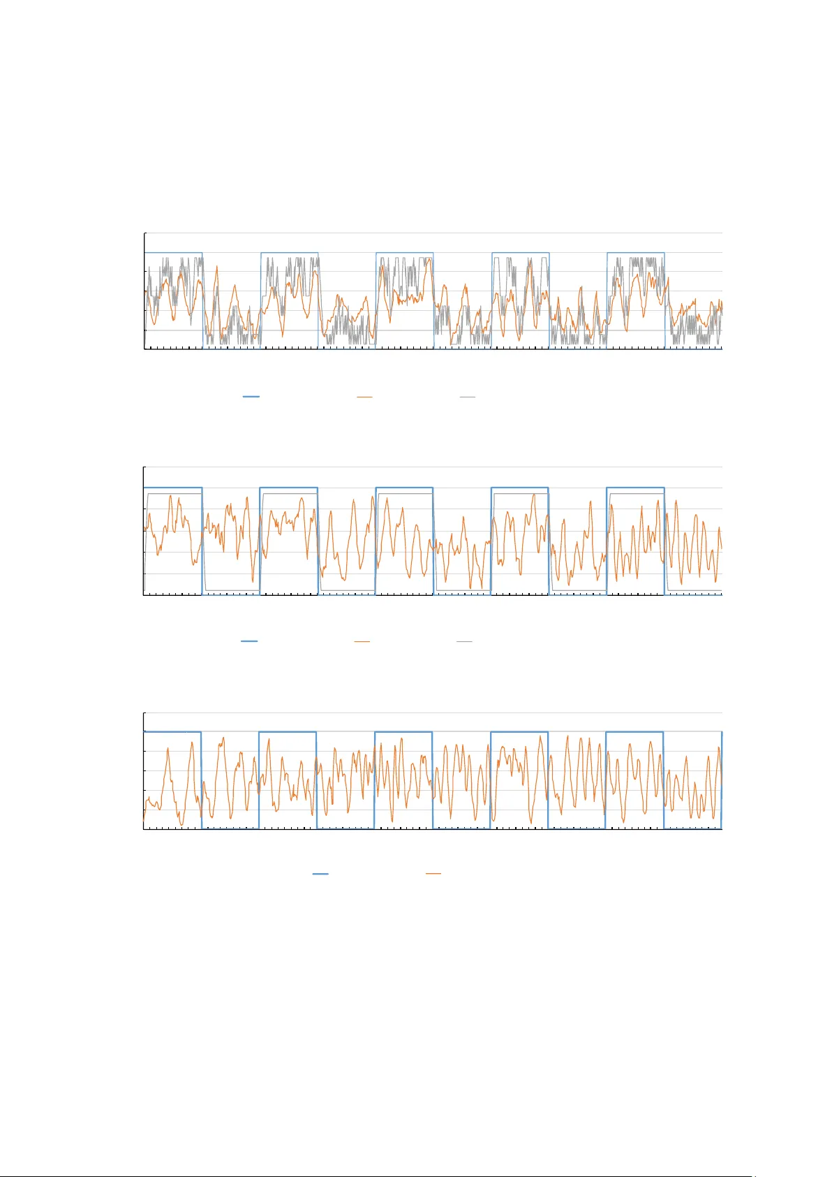
Con trolling Fish Sc ho ols via Reinforcemen t Learning of Virtual Fish Mo v emen t Y usuk e Nishii 1 and Hiroaki Ka washima ∗ 1,2 1 F acult y of Engineering, Ky oto Univ ersity , Ky oto, Japan 2 Graduate School of Informatics, Ky oto Univ ersity , Ky oto, Japan Note: This r ep ort pr esents an English tr anslation of the original Jap anese b achelor’s the- sis submitte d by Y usuke Nishii in 2018 to the Under gr aduate Scho ol of Ele ctric al and Ele c- tr onic Engine ering, F aculty of Engine ering, Kyoto University, under the sup ervision of Hir o aki Kawashima. The r ese ar ch was c onducte d b etwe en 2017 and 2018 while the authors wer e affili- ate d with Kyoto University. This tr anslation includes minor r evisions for clarity. The original thesis was c omplete d on F ebruary 9, 2018, and its c ontent r efle cts the state of r ese ar ch at that time. The tr anslation aims to pr eserve the me aning and structur e of the original work while making it ac c essible to a br o ader audienc e. The liter atur e r eview and the scientific c ontext of this work r efle ct the state of the field at the time of the original submission date. Abstract This study in vestigates a method to guide and control fish sc ho ols using virtual fish trained with reinforcement learning. W e utilize 2D virtual fish displa yed on a screen to o vercome tec hnical c hallenges such as durabilit y and mov ement constrain ts inherent in ph ys- ical robotic agents. T o address the lac k of detailed b eha vioral mo dels for real fish, we adopt a mo del-free reinforcement learning approach. First, simulation results show that re- inforcemen t learning can acquire effective mo vemen t p olicies ev en when simulated real fish frequen tly ignore the virtual stimulus. Second, real-world exp erimen ts with live fish confirm that the learned p olicy successfully guides fish sc h ools to ward sp ecified target directions. Statistical analysis reveals that the prop osed metho d significantly outp erforms baseline con- ditions, including the absence of stimulus and a heuristic “stay-at-edge” strategy . This study pro vides an early demonstration of how reinforcemen t learning can be used to influence collectiv e animal b eha vior through artificial agents. 1 In tro duction 1.1 Researc h Bac kground The long-term ob jectiv e of this researc h is to guide and con trol the mov ement of fish schools using externally con trolled rob otic agents. P otential applications range from choreographing fish sc ho ol tra jectories for aquarium exhibitions to na vigating sc ho ols in aquaculture settings. In such practical scenarios, the target fish schools are exp ected to b e relatively large, making it impractical to pro vide stim uli to every individual within the group. Consequently , it b ecomes necessary to control the en tire school b y stimulating only a limited n um b er of individuals. T o ac hieve this, it is crucial to pro vide stim uli tailored to the real-time state of the sc ho ol, for instance, b y iden tifying whic h individuals exert the strongest influence on the collective motion ∗ Presen t address: Graduate School of Information Science, Universit y of Hyogo, Kobe, Japan. Corresp onding author: k a wa shima@gsis.u-hy ogo.ac.jp 1 and determining how they should mov e to guide the group tow ard a desired ob jectiv e. This suggests that feedbac k con trol, whic h provides appropriate stim uli based on the evolving state of the school, is indisp ensable. A primary approac h to such con trol inv olv es the use of motion prediction mo dels for fish sc ho ols. These models would allo w for predicting the school’s resp onse to sp ecific stimuli and pre- ev aluating control strategies against desired targets. Regarding motion mo dels, previous studies, suc h as the one by Couzin et al. [ 1 ], hav e successfully simulated natural sc ho oling b eha viors and con tributed significan tly to elucidating collective mec hanisms. Ho wev er, at present, these mo dels ha ve not yet reached the level of accuracy required to predict the real-time mov ements of actual fish sc ho ols. 1.2 Researc h Ob jectiv es P otential stimuli for influencing fish b eha vior include predators, fo od, and artificial consp ecifics. Ho wev er, the use of predators is exp ected to cause significant stress to the target fish, while the con tinuous provision of fo o d can lead to health and en vironmental issues. Therefore, this study fo cuses exclusiv ely on the use of artificial consp ecifics as stimuli. T o address the challenge of not ha ving a predictive model for the target school’s mov emen t, we prop ose an approac h that acquires mov ement p olicies through reinforcement learning (RL) [ 2 ], with the artificial consp ecific serving as the RL agent. RL is a learning framew ork in which an agen t observes the state of the environmen t, determines an action based on that state, and receiv es a reward as an ev aluation of that action to acquire a near-optimal p olicy . This metho d offers the distinct adv antage of not requiring an explicit mo del of the environmen t (the target sc ho oling behavior). While the long-term goal is to implemen t these artificial consp ecifics as physical rob ots, con trolling the precise motion of the rob ots themselv es remains a significant c hallenge. T o circum ven t this, w e utilize virtual fish display ed on a screen. Virtual fish not only allow for easier motion control but also offer superior durabilit y compared to mec hanical robots. Since RL requires virtual fish to in teract with the sc ho ol ov er extended perio ds to acquire an effective p olicy , the durabilit y of virtual agents is highly suitable for the ob jectiv es of this study . Based on the ab o ve, this researc h aims to inv estigate a method for controlling fish schools b y applying RL to the mov ements of virtual fish. F or simplicit y , the scale of the fish sc ho ol is limited to a small n umber of individuals. 1.3 Related W ork V arious models hav e b een prop osed to describ e collective b eha vior in nature. Notable examples include the Kuramoto mo del [ 3 , 4 ], originally dev elop ed to explain the synchronization of firefly flashing; the Boids mo del [ 5 ], whic h sim ulates the flo c king behavior of birds; and the mo del b y Couzin et al. [ 1 ], whic h characterizes the collectiv e mov emen ts of fish sc ho ols. Sev eral studies hav e inv estigated schooling b eha vior by pro viding external stim uli to fish. F or instance, Sw ain et al. observ ed the reactions of fish to predator-lik e stim uli [ 6 ]. K opman et al. dev elop ed a rob otic consp ecific that adjusts its tail-fin motion based on the real-time positions of liv e fish to observ e their behavioral changes [ 7 ]. F urthermore, researc h has also fo cused on using visual stimuli to influence b eha vior. Kaw ashima et al. utilized a camera-display system to presen t virtual fish to a school, confirming that the real fish synchronized their mo vemen ts with the recipro cating motion of the virtual fish [ 8 ]. A fundamen tal biological reaction of fish to visual stim uli is the optomotor response. This is considered a reflexive b eha vior in which fish follo w a moving ob ject or pattern. A w ell-known exp erimen tal demonstration in v olves placing a cylinder with v ertical blac k-and-white strip es around a water tank; as the cylinder rotates, the fish swim along with the strip es [ 9 ]. Such 2 reflexiv e behaviors suggest the significan t potential for con trolling the mo vemen t of fish schools through precisely designed visual stim ulation. 1.4 Structure of the Rep ort The remainder of this rep ort is organized as follows. Section 2 describ es the problem formulation of this study and the configuration of the in teraction system b et ween the virtual fish and the real fish. Section 3 explains how the interaction system is mo deled as a Mark o v Decision Pro cess (MDP), a standard framew ork for representing agent-en vironment interactions in RL, and details the Q-learning algorithm emplo y ed in this study . Section 4 presen ts a preliminary ev aluation using simulations to verify whether RL remains effective even when simulated real fish frequen tly ignore the virtual fish. Section 5 discusses the implementation of RL in a real-world en vironment and ev aluates the p erformance of the acquired mov emen t p olicies. Finally , Section 6 concludes this study and suggests directions for future work. 2 In teraction System for Fish Sc ho ols and Virtual Fish 2.1 Problem F orm ulation F or simplicity , this study considers a fish school consisting of a small num b er of individuals of the same sp ecies. The target species should b e easy to obtain and maintain, and p ossess strong sc ho oling tendencies. T o satisfy these criteria, we use the Rummy-nose tetra ( Hemigr ammus bleheri 1 ). Generally , the p ositions of fish in a tank v ary freely in three-dimensional (3D) space. How ev er, in this study , the exp erimen ts are conducted in a narrow environmen t to treat the fish p ositions as tw o-dimensional (2D) coordinates. The internal dimensions of the tank used for housing and exp erimen ts are 34 . 0 cm in width, 14 . 0 cm in length (front-to-bac k distance), and 28 . 3 cm in heigh t. During exp erimen ts, partition plates are used to restrict the swimming area to 30 . 4 cm in width, 5 . 0 cm in length, and 12 . 5 cm in heigh t. A displa y is placed against the bac k of the tank to presen t virtual fish, and the in teraction is observ ed using a camera positioned in front of the tank. A sc hematic diagram of this system is sho wn in Fig. 1 . Details regarding the presentation of virtual fish and the camera-based observ ation are provided in Sections 2.2 and 2.3 , respectively . 2.2 Rationale for Using Vi rtual Fish First, w e discuss the justification for using virtual fish on a screen. Fish sc ho ols are formed through reactions b et ween individuals, categorized as follows: A ttraction: Individuals recognize consp ecifics visually and mov e tow ard each other. Alignmen t: Individuals follow the mo vemen ts of neigh b ors through the optomotor response. Repulsion: Individuals main tain distance from neigh b ors based on lateral line sensations to a void collisions. Among these, attraction leads to “aggregation,” where fish gather in close proximit y , and align- men t leads to the formation of a “sc ho ol,” where they mov e in a unified direction. Therefore, w e exp ect that the mov ement of the sc ho ol can b e controlled by inducing attraction and alignmen t, reactions primarily based on visual stimuli, using virtual fish. Indeed, it has b een rep orted that when a school of three Rummy-nose tetras w as presented with virtual fish p erforming p eriodic 1 Hemigr ammus bleheri has b een reclassified as Petitel la bleheri in 2020, while the original name is retained in this translation to maintain consistency with the 2018 source text. 3 Camera Fish tank Display Update the control strategy Controller Get the state of real fish school Decide the motion of virtual fish Reinforcement learning Real-time feedback system Figure 1: Ov erview of the in teraction system betw een a fish school and virtual fish. Figure 2: Image and arrangement of the virtual fish, including the background color. recipro cating motions via a camera-display system, the real fish tended to synchronize with the virtual ones [ 8 ]. Thus, the use of virtual fish is considered v alid. Next, w e consider the design of the virtual fish. Since the fron t-to-back dimension of the swimming area is restricted, w e place a displa y 2 against the bac k of the tank. As previously men tioned, attraction is triggered by visual recognition of consp ecifics. Therefore, it is effectiv e to use virtual fish that resemble the target sp ecies in shap e, size, and texture. Consequently , w e use an image created b y photographing real fish, as shown in Fig. 2 . The bac kground color is k ept uniform across the display . 2 ASUS MB168B (15.6-inch, resolution 1366 × 768 , pixel pitch 0 . 252 mm , resp onse time 11 ms , USB 3.0 inter- face). 4 Figure 3: Example of a captured image. Due to the light from the displa y , the real fish app ear dark as silhouettes. 2.3 Camera-Based Measuremen t of Fish Sc ho ols A camera 3 is p ositioned in fron t of the tank to capture the in teraction. The frame rate is set to 10 fps , which is sufficien t to capture the mo vemen ts of the fish. An example of a captured image is shown in Fig. 3 . W e define a “viewp ort” as a plane that collapses the front-to-bac k dimension within the restricted swimming area. Co ordinates within the viewp ort are expressed as ( x viewport , y viewport ) , normalized such that x viewport , y viewport ∈ [0 , 1] . The corresp ondence b et ween the captured image co ordinates ( x camera , y camera ) and the view- p ort co ordinates ( x viewport , y viewport ) is approximately expressed as: x viewport = a x camera + b, (1) y viewport = c y camera + d. (2) The constants a, b, c, d are obtained b y man ually selecting the four b oundaries corresp onding to the viewp ort in an image captured before the exp erimen t. Similarly , the relationship b et w een the viewport co ordinates and the display co ordinates ( x display , y display ) is approximated as: x display = e x viewport + f , (3) y display = g y viewport + h. (4) T o determine the constants e, f , g , h , tw o p oin ts with kno wn displa y co ordinates are sho wn b efore the experiment. Their positions in the captured image are man ually iden tified and con verted to viewp ort co ordinates using Eqs. ( 1 ) and ( 2 ). This allo ws us to calculate e, f , g , h using the corresp onding coordinate pairs in the displa y co ordinate system and the viewp ort coordinate system. Through this process, b oth the p ositions in the captured images and the p ositions on the displa y can b e represented consisten tly within the viewp ort co ordinate system. 3 Reinforcemen t Learning of Virtual Fish Mov emen t 3.1 Mark ov Decision Pro cess for Fish School Control First, we outline the general framew ork of RL based on Sutton and Barto [ 2 ]. In RL, the en tity that performs learning and decision-making is called the agent , and the entit y it in teracts 3 FLIR Flea 3 FL3-U3-13E4C-C (resolution 1280 × 1080 , color, max frame rate 60 fps , USB 3.0 interface), lens: FUJINON HF9HA-1B (ap erture F1.4–F16, fo cal length 9 mm ). 5       ! "   # "  ! "$%    & "$% Figure 4: In teraction b et ween the agen t and the en vironment in reinforcemen t learning. with is called the envir onment . The agen t and en vironment interact at eac h discrete time step n = 0 , 1 , . . . . Sp ecifically , the agent observ es a state s n ∈ S (where S is the state space) from the environmen t and, based on this, selects an action a n ∈ A (where A is the action space). By p erforming action a n , the agen t influences the environmen t, resulting in the observ ation of the next state s n +1 and a corresp onding reward r n +1 ∈ R . This interaction is illustrated in Fig. 4 . When the system satisfies the Mark o v prop ert y , that is, when s n +1 and r n +1 are determined probabilistically only b y s n and a n , the model is called a Mark ov Decision Pro cess (MDP). An MDP with finite sets S and A is kno wn as a finite MDP . In man y cases, RL aims to address situations that can b e appro ximated as finite MDPs. The goal of the agen t is to learn actions a n that maximize the long-term cumulativ e rew ard r n +1 , r n +2 , . . . , formulated as the maximization of the discounted return R n using a discount rate γ ∈ [0 , 1] : R n = ∞ X k =0 γ k r n + k +1 . (5) Here, we mo del the fish sc ho ol control problem for RL. F or simplicit y , we fo cus on controlling the x -coordinate, the primary direction of mo v emen t, while ignoring the y -co ordinate. The con trol ob jective is to guide the cen troid of the real fish school to ward the edges of the tank. The target direction is switched b et w een the left and righ t edges at appropriate in terv als. By assuming left-right symmetry , we consider that the p olicy learned to guide the school to ward one edge is equally effective for the opp osite direction. The discrete time step n corresponds to the time when the (10 n ) -th frame is captured by the camera; th us, the duration of eac h step is 1 s . Contin uous time is denoted by t , and the con tinuous time corresp onding to step n is denoted b y t n . Before defining S and A , w e define regions called c el ls within the viewp ort. Cells are defined b y dividing the viewp ort horizontally in to W in terv als. F or a giv en n umber of divisions W , a cell w ∈ { 0 , 1 , . . . , W − 1 } is defined in the viewp ort co ordinate system as:           x y      x ∈  w W , w + 1 W  , y ∈ [0 , 1]  when guiding tow ard the right edge,  x y      x ∈  W − w − 1 W , W − w W  , y ∈ [0 , 1]  when guiding tow ard the left edge. (6) This cell definition is illustrated in Fig. 5 . The state is defined as a pair of w real and w virtual , representing the cells con taining the cen troids of the real fish sc ho ol and that of the virtual fish, respectively . Thus, the state space is: S = { ( w real , w virtual ) | w real , w virtual ∈ { 0 , 1 , 2 , . . . , W − 1 }} . (7) 6  w = 0 $ = % − 1 $ = % − 1 w = 0 Figure 5: Definition of cells. When the num b er of divisions is W , the cell at the target end is defined as W − 1 , and the cell at the opp osite end is defined as 0 . Next, w e define the actions. The mo vemen t of the virtual fish at each step is determined as follo ws: Step 1: Determine the target p oin t x virtual - target . 1. Obtain the current centroid p ositions x real and x virtual . 2. Determine the cell w virtual con taining x virtual . 3. Select a cell displacement ∆ w ∈ { 0 , ± 1 , ± 2 , . . . , ± ∆ w max } . 4. Set the target cell w virtual - target : ˜ w virtual - target = w virtual + ∆ w (8) w virtual - target =      0 if ˜ w virtual - target < 0 , ˜ w virtual - target if 0 ≤ ˜ w virtual - target ≤ W − 1 , W − 1 if W − 1 < ˜ w virtual - target . (9) 5. Using the x -coordinate center of w virtual - target ( x virtual - target ) and the y -co ordinate of the real fish centroid ( y real ), set the target p oin t: x virtual - target =  x virtual - target y real  . (10) Step 2: Mov e to ward the target p oin t until the next step. The cen troid follows a first-order lag motion: d x virtual d t = 1 τ virtual ( x virtual - target − x virtual ) , (11) 1 τ virtual > 0 ( constan t ) . (12) Since the motion of the virtual fish is determined by ∆ w , we define ∆ w as the action. Thus, the action space is: A = { 0 , ± 1 , ± 2 , . . . , ± ∆ w max } . (13) Finally , the reward r n is defined based on the x -co ordinate of the real fish sc ho ol cen troid x real at step n : r n = ( 2 × ( x real − 0 . 5) when guiding tow ard the right edge, 2 × (0 . 5 − x real ) when guiding to ward the left edge. (14) Th us, r n ∈ [ − 1 , +1] , and r n approac hes +1 as the centroid x real gets closer to the target edge. 7 3.2 Reinforcemen t Learning via Q-Learning In this section, we describ e the Q-learning algorithm, based again on Sutton and Barto [ 2 ]. The agen t’s actions are determined probabilistically according to a p olicy π . The probability distribution of action a n giv en state s n is: a n ∼ π ( ·| s n ) , (15) where π ( a | s ) represen ts the probability of c ho osing action a in state s . The exp ected discounted return when following p olicy π from state s is defined as the state-v alue function: V π ( s ) = E π { R n | s n = s } . (16) The optimal p olicy π ∗ is defined as the p olicy satisfying π ∗ ∈ arg max π V π ( s ) (17) for all s ∈ S . The goal of RL is to acquire π ∗ . Giv en the optimal action-v alue function Q ∗ ( s, a ) = max π Q π ( s, a ) , where Q π ( s, a ) = E π { R n | s n = s, a n = a } , the optimal p olicy can be obtained as: π ∗ ( a | s ) =    1 | arg max a ′ Q ∗ ( s, a ′ ) | if a ∈ arg max a ′ Q ∗ ( s, a ′ ) , 0 otherwise. (18) Based on the Bellman optimalit y equation, Q ∗ ( s, a ) = E  r n +1 + γ max a ′ Q ∗ ( s n +1 , a ′ )     s n = s, a n = a  , (19) the function Q ( s n , a n ) can be up dated iterativ ely to appro ximate Q ∗ b y making it conv erge to ward r n +1 + γ max a ′ Q ( s n +1 , a ′ ) . The learned p olicy π corresp onding to this approximated Q is expressed as: π ( a | s ) =    1 | arg max a ′ Q ( s, a ′ ) | if a ∈ arg max a ′ Q ( s, a ′ ) , 0 otherwise. (20) Q-learning implements this through the follo wing pro cedure: Step 1: Initialize the action-v alue function Q and observe the initial state s 0 . Step 2: Rep eat for each step n = 0 , 1 , . . . , N − 1 : 1. Select action a in state s based on the policy π n deriv ed from Q . 2. Execute action a and observ e reward r and next state s ′ . 3. Up date Q according to: Q ( s, a ) ← Q ( s, a ) + α  r + γ max a ′ Q ( s ′ , a ′ ) − Q ( s, a )  , (21) α ∈ (0 , 1) ( constant, called the “step size” ) . (22) 4. s ← s ′ Regarding π n , it is effective to p erform explor ation (trying v arious actions) in the early stages of learning and follow the b est-kno wn p olicy in the later stages. Thus, we use an ϵ -greedy algorithm where ϵ is decay ed at each step: ϵ n = 1 − n N − 1 (23) π n ( a | s ) =        1 − ϵ n | arg max a ′ Q ( s, a ′ ) | + ϵ n |A| if a ∈ arg max a ′ Q ( s, a ′ ) , ϵ n |A| otherwise. (24) 8 4 Preliminary Ev aluation in a Sim ulation En vironmen t When in teracting with a fish school using virtual fish, the frequency with which the real fish react to the virtual fish is exp ected to b e limited. T o inv estigate whether an effective policy can b e acquired via RL under suc h conditions, w e p erform RL in a simulation environmen t that mimics the mov ement of real fish. F urthermore, as will b e discussed in Section 5 , learning an effective p olicy in an actual inter- action system is expected to be extremely time-consuming. By using the action-v alue function Q obtained in the sim ulation en vironment, where each time step can b e processed muc h faster than in the real environmen t, as an initial v alue, we exp ect to reduce the learning time required in the real-world exp erimen ts. 4.1 Mo deling the Mov emen t of Real Fish W e sim ulate the b eha vior of real fish using an action mo del in whic h the decision to react to the virtual fish is determined probabilistically . By v arying this probability , we examine whether RL can acquire effective p olicies even when real fish infrequently react to virtual fish. Based on observ ations of the fish during housing, the following b eha vioral c haracteristics were iden tified: • They sho w minimal reaction to other individuals that are far a w ay . • When they do react to another individual, they often begin swimming to ward that indi- vidual. • Most of their mov ements can b e view ed as a repetition of linear motions lasting for a few seconds. W e dev elop ed a mo del for real fish that reflects these prop erties. F or simplicit y , we assume that the real fish alwa ys act as a collective school and simulate the motion of their centroid. The follo wing parameters are held constant within eac h simulation: • ∆ t max > 0 : Maxim um duration b efore the real fish switch their target p oin t. • θ > 0 : Maxim um distance at whic h real fish react to the virtual fish. • p ∈ [0 , 1] : Probability that the real fish ignore the virtual fish even when they are sufficiently close. • δ x max > 0 , δ y max > 0 : Maxim um displacement of the target point when the virtual fish are ignored. • 1 /τ real > 0 : In verse of the time constant for the first-order lag system of the real fish. Let x real =  x real y real  and x virtual represen t the cen troid p ositions of the real fish sc ho ol and the virtual fish, resp ectiv ely . The motion of x real is mo deled as a series of mo vemen ts tow ard a switc hing target p oin t x real - target , eac h of whic h is gov erned b y a first-order lag system, sim ulated as follo ws: Step 1: Randomly select a duration ∆ t ∈ (0 , ∆ t max ] for which the fish mo ve linearly . Step 2: Determine the target p oin t x real - target as follows: • If ∥ x virtual − x real ∥ ≤ θ : 9 – With probabilit y 1 − p (reaction case), set: x real - target = x virtual . (25) – With probabilit y p (ignore case), select random relativ e displacemen ts δ x ∈ [ − δ x max , + δ x max ] and δ y ∈ [ − δ y max , + δ y max ] , and set: x real - target = x real +  δ x δ y  . (26) • Otherwise (out of range): Determine x real - target using random displacemen ts as in Eq. ( 26 ). Step 3: During the in terv al ∆ t , mov e to w ard x real - target based on d x real d t = 1 τ real ( x real - target − x real ) . (27) Step 4: Rep eat Steps 1 through 3. 4.2 Ev aluation of Robustness Against Sto c hastic Beha vior 4.2.1 Sim ulation Ev aluation Conditions W e ev aluate whether RL can acquire effective mo vemen t policies even in scenarios where real individuals infrequently respond to the virtual stimulus. T o this end, we conduct RL for each ignoring probabilit y p defined in the b eha vioral mo del in Section 4.1 . W e then inv estigate whether the resulting p olicy approximates the optimal policy b y analyzing the rewards obtained when follo wing this p olicy . F or eac h ignoring probabilit y p = 0 , 0 . 3 , 0 . 6 , 0 . 9 , Q-learning is performed with the n um b er of training steps N v aried across { 10 2 , 10 3 , 10 4 , 10 5 , 10 6 , 10 7 } . Other parameter settings are summarized in T able 1 . After training, the agent follo ws the learned p olicy π (as defined in Eq. ( 20 )) for M steps to calculate the av erage reward R : R = 1 M M X n =0 r n , (28) where M = 9000 . Since b oth the learned p olicy and the resulting rew ard R are inheren tly sto c hastic, we expect the ev aluation R to v ary across trials. Therefore, w e rep eat the training and ev aluation pro cess 10 times for eac h com bination of p and N , and calculate the mean of R across these trials. Note that the rew ard R obtained under an optimal p olicy v aries dep ending on the ignoring probabilit y p . T o pro vide a benchmark for ev aluating the learned p olicies, w e define a heuris- tic policy ˆ π that is expected to yield near-optimal rew ards. In this simulation, the maximum in teraction distance θ (the range within whic h real fish react to the virtual fish) is set to 0.3 times the viewport width, and the num b er of cell divisions is W = 10 . Consequen tly , a policy ˆ π that targets a p osition three cells ahead of the real fish’s current cell w real (i.e., w real + 3 ) is considered near-optimal. Sp ecifically , given a state ( w real , w virtual ) , the baseline p olicy ˆ π is defined as follows: ∆ ˜ w = w real + 3 − w virtual . (29) ∆ w =      − ∆ w max if ∆ ˜ w < − ∆ w max , ∆ ˜ w if − ∆ w max ≤ ∆ ˜ w ≤ ∆ w max , +∆ w max if ∆ w max < ∆ ˜ w . (30) ˆ π ( a | s ) = ( 1 if a = ∆ w, 0 otherwise. (31) 10 T able 1: Simulation parameters. θ and δ x max are relativ e to the viewport width, and δ y max is to the viewp ort height. P arameter Description V alue γ Discoun t factor (Q-learning) 0.9 α Step size (Learning rate) (Q-learning) 0.1 W Num b er of cells 10 ∆ w max Max cell displacement p er step (virtual fish) 2 1 /τ virtual In verse time constant (virtual fish) 3 s − 1 ∆ t max Max duration for target switc hing (real fish) 3 s θ Max reaction distance (real fish) 0.3 δ x max Max x -displacement during ignore cases (real fish) 0.2 δ y max Max y -displacement during ignore cases (real fish) 0.2 1 /τ real In verse time constant (real fish) 1 s − 1 -0 . 1 0 0. 1 0. 2 0. 3 0. 4 0. 5 0. 6 0. 7 0. 8 0. 9 1 1 10 10 0 10 00 10 00 0 10 00 00 10 00 00 0 10 00 00 00 R (average of 10 training) N p = 0.0 p = 0.0 ( baseline ) p = 0.3 p = 0.3 ( baseline ) p = 0.6 p = 0.6 ( baseline ) p = 0.9 p = 0.9 ( baseline ) Figure 6: A v erage reward R in simulation. p represen ts the probability of the sim ulated real fish ignoring the virtual fish. The baseline denotes the reward obtained using ˆ π as defined in Eq. ( 31 ). Here, the maximum displacement of the virtual fish’s cell p er step is set to ∆ w max = 2 , consistent with the constraints of the RL agent. W e denote the rew ard obtained by this baseline p olicy ˆ π o ver M = 9000 steps as ˆ R . Since ˆ R is also expected to v ary across trials, we calculate ˆ R 10 times for eac h p and take the mean. If the mean reward R of a learned p olicy is sufficien tly close to the mean b enc hmark ˆ R , we consider the acquired p olicy to b e near-optimal. 4.2.2 Results and Discussion of Simulation Ev aluation The results of the ev aluation described in Section 4.2.1 are shown in Fig. 6 . Regardless of the ignoring probabilit y p , it can b e observed that as the num b er of training steps N increases, the a verage reward R obtained under the learned p olicy approaches the reward ˆ R obtained under the baseline p olicy ˆ π . Figure 7 shows the ratio of the mean rew ard R under the learned p olicy to the mean reward ˆ R under the baseline p olicy . F or ignoring probabilities p = 0 , 0 . 3 , and 0 . 6 , the ratio reaches 11 -0 . 1 0 0. 1 0. 2 0. 3 0. 4 0. 5 0. 6 0. 7 0. 8 0. 9 1 1. 1 1 10 10 0 10 00 10 00 0 10 00 00 10 00 00 0 10 00 00 00 R / R -baseline N p = 0. 0 p = 0. 3 p = 0. 6 p = 0. 9 Figure 7: Ratio of the av erage reward of the learned p olicy to that of the baseline p olicy in sim ulation. p represents the probabilit y of the sim ulated real fish ignoring the virtual fish. appro ximately 1.0 when the n um b er of training steps N is sufficien tly large. This suggests that the learned p olicies in these cases are nearly optimal. F urthermore, even in the case of p = 0 . 9 , where the real fish ignore the virtual stim ulus with high frequency , the ratio reac hes appro ximately 0.7 at N = 10 7 , indicating that learning progresses to a certain extent even under suc h challenging conditions. 5 Reinforcemen t Learning in a Real-W orld Environmen t 5.1 A cquisition of Cen troid P ositions for Real and Virtual Fish The centroid p osition of the real fish is determined as follows . F or an RGB color image, let p u,v =   r u,v g u,v b u,v   represen t the pixel at column u and row v . The entire image is denoted as { p u,v } , where r u,v , g u,v , and b u,v are the red, green, and blue v alues at p osition ( u, v ) . F or a gra yscale image, the pixel v alue is denoted as p u,v , and the image as { p u,v } . Step 1: A binary image is obtained using background subtraction. Given a pre-recorded bac k- ground image { ˜ p u,v } and a threshold θ , w e compute for each ( u, v ) : p ′ u,v = ( 1 if ∥ p u,v − ˜ p u,v ∥ > θ , 0 otherwise. (32) The resulting binary image  p ′ u,v  is exp ected to hav e a v alue of 1 where real or virtual fish are present, and 0 elsewhere. Step 2: As shown in Fig. 3 , real fish app ear as dark silhouettes due to the displa y’s backligh ting. This color difference is used to distinguish b et w een real and virtual fish. Using a decision function f obtained via a Supp ort V ector Mac hine (SVM), we compute: p ′′ u,v = ( 1 if p ′ u,v = 1 and f ( p u,v ) > 0 , 0 otherwise. (33) 12 T able 2: P arameters for RL and control in the real-w orld environmen t. P arameter Description V alue γ Discoun t factor (Q-learning) 0.9 α Step size (Learning rate) (Q-learning) 0.1 W Num b er of cell divisions 10 ∆ w max Max cell displacement p er step (virtual fish) 2 1 /τ virtual In verse time constant (virtual fish) 1 s − 1 The SVM is pre-trained on a dataset where f ( p ) is +1 for real fish pixels and − 1 for virtual fish pixels. Step 3: The binary image  p ′′ u,v  is pro cessed with an op ening op eration (an equal num b er of erosions and dilations) to obtain  p ′′′ u,v  . This ensures that pixels with a v alue of 1 corresp ond only to the real fish. Step 4: The cen troid ˜ x real of the pixels with v alue 1 in  p ′′′ u,v  is calculated as: ˜ x real = m 1 , 0 m 0 , 0 m 0 , 1 m 0 , 0 ! where m i,j = X u,v u i v j p ′′′ u,v . (34) Finally , ˜ x real is conv erted to viewp ort co ordinates x real using Eqs. ( 1 ) and ( 2 ). Step 3 is a pro cedure designed to eliminate misclassifications originating from the SVM in Step 2. Sp ecifically , classification errors o ccasionally caused certain subregions to b e mark ed as contain- ing a real fish ( p ′′ u,v = 1 ) ev en when no fish was present. By implemen ting Step 3, we successfully remo ved most of these false p ositiv es. Regarding the position of the virtual fish cen troid, w e set the time constan t τ imitated of the first-order lag system in Eq. ( 11 ) to b e sufficiently small so that the mov ement sp eed is high enough. This allows us to assume that the virtual fish reac h sufficien tly close to their target p oin t x virtual - target within a single time step. Consequently , the p osition of the virtual fish centroid at an y given time is treated as the target p oin t selected in the preceding state. 5.2 Ev aluation of the Learned P olicy W e inv estigate whether RL can yield an effectiv e mo vemen t p olicy for virtual fish to guide fish sc ho ols in a real-w orld environmen t. Our analysis is based on the b eha vior of b oth real and virtual individuals under the learned policy . Since training in a real-world environmen t is expected to b e extremely time-consuming, w e initialize the action-v alue function Q using the v alues obtained from simulation (with an ignoring probabilit y p = 0 . 6 and N = 10 6 steps) to shorten the required training duration. Reinforcemen t learning w as conducted for N = 1800 steps. The parameter settings are summarized in T able 2 . Three randomly selected real fish were used for the experiment. Sub- sequen tly , 900 steps of control were p erformed on the same individuals following the learned p olicy (hereafter referred to as the “prop osed metho d”). W e verify whether the prop osed metho d successfully guides the real individuals tow ard the target direction and determine if it is more effectiv e than a simple, manually defined p olicy . W e therefore inv estigated the b eha vior of real individuals for 900 steps under the following baselines: Baseline 1 (stay at edge): The virtual fish mov e tow ard the target direction and stays at the edge of the viewp ort once it reac hes it. Baseline 2 (w/o stimulus): No virtual fish are display ed. 13 T able 3: Mean real fish x -co ordinates for each guidance direction and the difference b et ween them for each control metho d. Condition (a) T arget: Left (b) T arget: Righ t Difference (b-a) Prop osed Metho d 0 . 358 0 . 525 0 . 166 Baseline 1 (stay at edge) 0 . 461 0 . 562 0 . 101 Baseline 2 (w/o stimulus) 0 . 501 0 . 495 − 0 . 006 T able 4: Results of the significance tests for the difference in the mean x -co ordinates of real fish based on the target guidance direction. A tw o-tailed W elc h’s t -test was performed for eac h virtual fish control metho d to ev aluate the statistical significance of the difference. Condition p -v alue Prop osed Metho d 1 . 46 × 10 − 51 Baseline 1 (stay at edge) 8 . 48 × 10 − 15 Baseline 2 (w/o stimulus) 5 . 80 × 10 − 1 Here, the p olicy for Baseline 1 w as defined as follo ws, with the maxim um displacement p er step set to ∆ w max = 2 to remain consistent with the prop osed metho d: π ( a | s ) = ( 1 if a = +∆ w max , 0 otherwise. (35) The reactions of real fish to the virtual fish are exp ected to b e influenced b y the preceding mo vemen ts of the virtual stimuli. Therefore, to av oid carry-ov er effects from previous trials, a rest p eriod of at least 10 minutes was provided b et ween the training phase, the ev aluation of the prop osed metho d, and eac h baseline exp erimen t. The cen troids of b oth real and virtual fish were recorded at each time step and are summarized in Fig. 8 . In the prop osed metho d, the virtual fish mo ve within the area b et ween the target p osition and the area near the real fish, app earing to guide the real individuals tow ard the goal. W e then generated histograms of the p ositions of real individuals (cen troids) for each target guidance direction. Figures 9 , 10 , and 11 sho w the results for the Prop osed Metho d, Baseline 1, and Baseline 2, resp ectiv ely . T able 3 summarizes the mean p ositions and the differences b et ween them for eac h target direction. A comparison reveals that the magnitude of the difference in mean p ositions follo ws the order: (a) the Proposed Metho d, (b) Baseline 1 (stay at edge), and (c) Baseline 2 (w/o stim ulus). The histograms also appear to b e sharp er in the same order. W e conducted W elc h’s t -test (tw o-tailed) at a significance level of 5 % to determine whether the target direction resulted in a significant difference in the mean p ositions of real individuals. The sample was defined as { x real ( t n ) | guided to x = 0 (or x = 1) at step n } , (36) assuming an appro ximately normal distribution. The resulting p -v alues are shown in T able 4 . These v alues indicate that while there was no significant difference in (c) Baseline 2, significant differences w ere observed in b oth (a) the Proposed Metho d and (b) Baseline 1. Th us, it can b e concluded that the real individuals w ere significantly guided in the intended directions in b oth (a) and (b). F urthermore, we ev aluated the degree of difference b et ween the histograms of the x -co ordinates for each target direction (Figs. 9 to 11 ) using the Bhattac haryy a distance. As sho wn in Fig. 12 , the results confirm that the difference in the distribution of the real individuals’ p ositions follows 14 0 0. 2 0. 4 0. 6 0. 8 1 1. 2 0 15 30 45 60 75 90 10 5 12 0 13 5 15 0 16 5 18 0 19 5 21 0 22 5 24 0 25 5 27 0 28 5 30 0 31 5 33 0 34 5 36 0 37 5 39 0 40 5 42 0 43 5 45 0 46 5 48 0 49 5 51 0 52 5 54 0 55 5 57 0 58 5 60 0 61 5 63 0 64 5 66 0 67 5 69 0 70 5 72 0 73 5 75 0 76 5 78 0 79 5 81 0 82 5 84 0 85 5 87 0 88 5 90 0 Centroid position x Target direction Time step n Virtual fish Real fish (a) Prop osed Metho d 0 0. 2 0. 4 0. 6 0. 8 1 1. 2 0 15 30 45 60 75 90 10 5 12 0 13 5 15 0 16 5 18 0 19 5 21 0 22 5 24 0 25 5 27 0 28 5 30 0 31 5 33 0 34 5 36 0 37 5 39 0 40 5 42 0 43 5 45 0 46 5 48 0 49 5 51 0 52 5 54 0 55 5 57 0 58 5 60 0 61 5 63 0 64 5 66 0 67 5 69 0 70 5 72 0 73 5 75 0 76 5 78 0 79 5 81 0 82 5 84 0 85 5 87 0 88 5 90 0 Centroid position x Target direction Time step n Virtual fish Real fish (b) Baseline 1 (stay at edge) 0 0. 2 0. 4 0. 6 0. 8 1 1. 2 0 15 30 45 60 75 90 10 5 12 0 13 5 15 0 16 5 18 0 19 5 21 0 22 5 24 0 25 5 27 0 28 5 30 0 31 5 33 0 34 5 36 0 37 5 39 0 40 5 42 0 43 5 45 0 46 5 48 0 49 5 51 0 52 5 54 0 55 5 57 0 58 5 60 0 61 5 63 0 64 5 66 0 67 5 69 0 70 5 72 0 73 5 75 0 76 5 78 0 79 5 81 0 82 5 84 0 85 5 87 0 88 5 90 0 Centroid position x Time step n Target direction Real fish (c) Baseline 2 (w/o stimulus) Figure 8: Time series of the x -coordinate of the real fish centroid during real-w orld control. 15 0 10 20 30 40 50 60 0. 0 0 0. 0 4 0. 0 8 0. 1 2 0. 1 6 0. 2 0 0. 2 4 0. 2 8 0. 3 2 0. 3 6 0. 4 0 0. 4 4 0. 4 8 0. 5 2 0. 5 6 0. 6 0 0. 6 4 0. 6 8 0. 7 2 0. 7 6 0. 8 0 0. 8 4 0. 8 8 0. 9 2 0. 9 6 1. 0 0 Frequency Horizontal position of the real fish centroid x direction = 0 (mean = 0.358) (a) Guiding tow ard the left ( x = 0 ) 0 10 20 30 40 50 60 0. 0 0 0. 0 4 0. 0 8 0. 1 2 0. 1 6 0. 2 0 0. 2 4 0. 2 8 0. 3 2 0. 3 6 0. 4 0 0. 4 4 0. 4 8 0. 5 2 0. 5 6 0. 6 0 0. 6 4 0. 6 8 0. 7 2 0. 7 6 0. 8 0 0. 8 4 0. 8 8 0. 9 2 0. 9 6 1. 0 0 Frequency Horizontal position of the real fish centroid x direction = 1 (me an = 0.525) (b) Guiding tow ard the right ( x = 1 ) Figure 9: Histograms of real fish x -coordinates (Proposed Metho d). Orange bins indicate the mean v alue’s interv al. 16 0 10 20 30 40 50 60 0. 0 0 0. 0 4 0. 0 8 0. 1 2 0. 1 6 0. 2 0 0. 2 4 0. 2 8 0. 3 2 0. 3 6 0. 4 0 0. 4 4 0. 4 8 0. 5 2 0. 5 6 0. 6 0 0. 6 4 0. 6 8 0. 7 2 0. 7 6 0. 8 0 0. 8 4 0. 8 8 0. 9 2 0. 9 6 1. 0 0 Frequency Horizontal position of the real fish centroid x direction = 0 (mean = 0.461) (a) Guiding tow ard the left ( x = 0 ) 0 10 20 30 40 50 60 0. 0 0 0. 0 4 0. 0 8 0. 1 2 0. 1 6 0. 2 0 0. 2 4 0. 2 8 0. 3 2 0. 3 6 0. 4 0 0. 4 4 0. 4 8 0. 5 2 0. 5 6 0. 6 0 0. 6 4 0. 6 8 0. 7 2 0. 7 6 0. 8 0 0. 8 4 0. 8 8 0. 9 2 0. 9 6 1. 0 0 Frequency Horizontal position of the real fish centroid x direction = 1 (mean = 0.562) (b) Guiding tow ard the right ( x = 1 ) Figure 10: Histograms of real fish x -coordinates (Baseline 1: stay at edge). 17 0 10 20 30 40 50 60 0. 0 0 0. 0 4 0. 0 8 0. 1 2 0. 1 6 0. 2 0 0. 2 4 0. 2 8 0. 3 2 0. 3 6 0. 4 0 0. 4 4 0. 4 8 0. 5 2 0. 5 6 0. 6 0 0. 6 4 0. 6 8 0. 7 2 0. 7 6 0. 8 0 0. 8 4 0. 8 8 0. 9 2 0. 9 6 1. 0 0 Frequency Horizontal position of the real fish centroid x direction = 0 (mean = 0.501) (a) Guiding tow ard the left ( x = 0 ) 0 10 20 30 40 50 60 0. 0 0 0. 0 4 0. 0 8 0. 1 2 0. 1 6 0. 2 0 0. 2 4 0. 2 8 0. 3 2 0. 3 6 0. 4 0 0. 4 4 0. 4 8 0. 5 2 0. 5 6 0. 6 0 0. 6 4 0. 6 8 0. 7 2 0. 7 6 0. 8 0 0. 8 4 0. 8 8 0. 9 2 0. 9 6 1. 0 0 Frequency Horizontal position of the real fish centroid x direction = 1 (mean = 0.495) (b) Guiding tow ard the right ( x = 1 ) Figure 11: Histograms of real fish x -coordinates (Baseline 2: w/o stim ulus). 18 0 0. 0 2 0. 0 4 0. 0 6 0. 0 8 0. 1 0. 1 2 0. 1 4 0. 1 6 0. 1 8 Proposed Baseline 1 (stay at edge) Baseline 2 (w/o stimulus) B h attacharyya distance between histograms Stimulus condition Figure 12: Distances b et ween the x -co ordinate distributions of real fish for left w ard and right ward guidance. F or each pair of histograms in Figs. 9 to 11 , the effectiveness of the guidance was quan tified by calculating the Bhattac haryya distance b et w een the distributions resulting from the tw o target directions. the order: (a) the Prop osed Metho d, (b) Baseline 1 (stay at edge), and (c) Baseline 2 (w/o stim ulus). Consequently , it is evident that the Prop osed Metho d (a) guided the real individuals more prominently than Baseline 1 (b). 6 Conclusion In this study , we in vestigated whether effective mo vemen t p olicies for virtual fish to guide fish sc ho ols could b e acquired through reinforcemen t learning (RL). First, there was a concern regarding whether RL could yield effectiv e p olicies in scenarios where the frequency of real fish resp onding to virtual stim uli is not necessarily high. T o address this, we established a b eha vioral mo del in which real individuals sto c hastically decide whether to follo w or ignore virtual fish when they are sufficiently close. Our simulation results confirmed that reasonably effectiv e p olicies could b e obtained even when the probabilit y of real individuals ignoring the virtual stimuli w as high. Second, w e v erified the feasibility of fish guidance in a real-world environmen t using the learned p olicy . The results demonstrated that when the virtual fish mov ed based on the learned p olicy , the mean positions of the real fish (cen troids) differed significantly dep ending on the target guidance direction. This confirms that the real individuals were successfully guided in the in tended directions. F urthermore, we compared the learned p olicy with a man ual baseline p olicy where the virtual fish simply mov e to and sta y at the edge of the viewp ort in the target direction. This comparison revealed that the distribution of the real fish’s p ositions changed more prominen tly under the control of the learned p olicy than under the simple manual policy . These findings confirm that RL can acquire a more effective p olicy than a simple, human-defined one. While this study demonstrated the p oten tial of RL-based fish sc ho ol control, sev eral issues remain for future inv estigation. V alidation of image-based stim uli as virtual fish: In this study , we used textures of real individuals for the visual stimuli. Ho wev er, it remains unclear whether these stimuli are 19 recognized by real fish as actual members of their school. T o clarify this, it is necessary to in vestigate whether b eha vioral resp onses differ when presen ting abstract stimuli, such as strip ed patterns or random dots, compared to the texture-mapp ed virtual fish used in our exp erimen ts. In vestigation of the n umber of individuals In this study , the num b ers of b oth virtual and real fish were fixed throughout the exp erimen ts. How ev er, tow ard the future goal of guiding large-scale sc ho ols with a small n um b er of virtual or rob otic agents, it is necessary to examine how the in teraction dynamics c hange when the resp ectiv e num b ers of real and virtual individuals are v aried. Examination of state representation in RL The state defined in this study was based on the resp ectiv e centroids of the real fish sc ho ol and the virtual fish group. Ho wev er, ev en if the sc ho ol is at the same position, the optimal action is exp ected to differ dep ending on whether the school is mo ving to ward or a wa y from the target direction. Therefore, p oten tial improv emen ts include incorporating information regarding the school’s velocity in to the state represen tation. F urthermore, for the future goal of in teracting with only a subset of individuals within a large-scale school, it will b e necessary to target sp ecific individuals that exert a significan t influence on the collectiv e motion. Defining the state in such scenarios w ould require incor- p orating more microscopic information, suc h as the spatial relationships among individuals and the status or strength of inter-individual interactions. On the other hand, there is a trade-off where the training duration for RL increases as the size of the state space grows. Therefore, it is necessary to devise metho ds to incorp orate the aforementioned information while effectiv ely managing the num b er of elemen ts in the state set. Examination of action representation in RL In the exp erimen ts conducted in this study , the mo vemen t of the four virtual fish w as designed such that they mo ved as a single co ordinated unit while main taining their relativ e positions. Ho wev er, to ac hieve more effectiv e in teractions with the same n umber of agen ts, it is expected that ha ving eac h virtual fish mo v e independently to interact with differen t individuals within the school w ould b e more efficient. On the other hand, similar to the challenges faced with the state space, it is necessary to de- vise metho ds that enable indep enden t mo vemen t for each virtual fish while simultaneously limiting the size of the action space to a manageable level. Ethical Appro v al All animal exp erimen ts were conducted with the approv al of the Graduate School of Informatics, Ky oto Universit y (Appro v al No. Inf-K17007, Marc h 21, 2017). References [1] I. D. Couzin, J. Krause, R. James, G. D. Ruxton, and N. R. F ranks, Collectiv e memory and spatial sorting in animal groups, Journal of the or etic al biolo gy , V ol. 218, No. 1, (2002), pp. 1–11. [2] R. S. Sutton and A. G. Barto, R einfor c ement L e arning : A n Intr o duction , MIT Press, (1998). 20 [3] Y. Kuramoto, Self-en traimen t of a p opulation of coupled nonlinear oscillators, International Symp osium on Mathematic al Pr oblems in The or etic al Phy sics (ed. H. Araki), V ol. 39, (1975), pp. 420–422. [4] F. A. Ro drigues, T. K. D. P eron, P . Ji, and J. Kurths, The kuramoto mo del in complex net works, Physics R ep orts , V ol. 610, (2016), pp. 1–98. [5] C. W. Reynolds, Flocks, herds, and schools: A distributed b eha vioral mo del, Computer Gr aphics , V ol. 21, No. 4, (1987), pp. 25–34. [6] D. T. Swain, I. D. Couzin, and N. E. Leonard, Real-time feedbac k-controlled rob otic fish for b eha vioral experiments with fish sc ho ols, Pr o c e e dings of the IEEE , V ol. 100, No. 1, (2012), pp. 150–163. [7] V. Kopman, J. Laut, G. Polv erino, and M. Porfiri, Closed-lo op control of zebrafish resp onse using a bioinspired rob otic-fish in a preference test, Journal of The R oyal So ciety Interfac e , V ol. 10, No. 78, (2013). [8] H. Ka washima, Y. Kanec hik a, and T. Matsuy ama, Camera-display system for the in terac- tion analysis of liv e fish vs fish-like graphics, The 17th Me eting on Image R e c o gnition and Understanding (MIRU 2014) , (2014). [9] G. P . Arnold, Rheotropism in fishes, Biolo gic al R eviews , V ol. 49, No. 4, (1974), pp. 515–576. 21