Exact Cost-Increment Formula for Optimal Control of Semilinear Evolution Equations

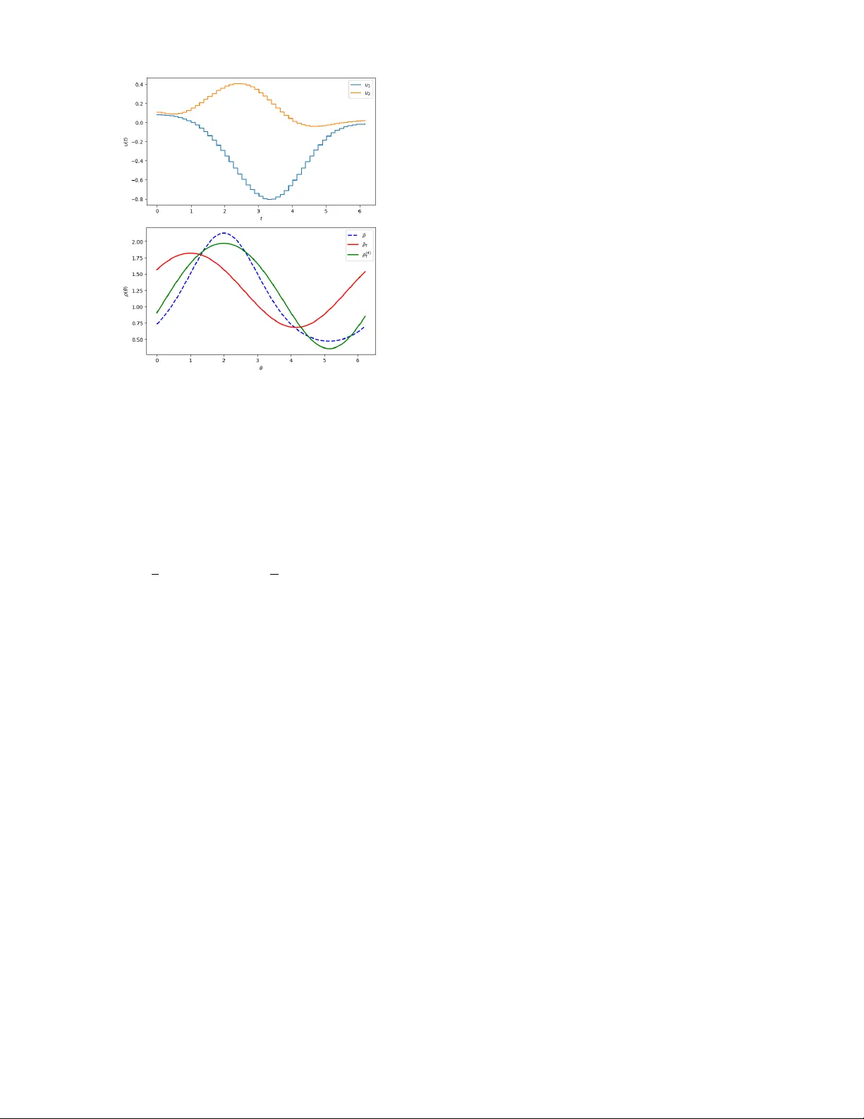
Exact Cost-Incr ement F ormula f or Optimal Contr ol of Semilinear Evolution Equations ∗ Roman Chertovskih, Nik olay Pogodae v , Maxim Staritsyn, and A. Pedro Aguiar , Member , IEEE - Abstract — W e address optimal contr ol of semilinear ev olution equations on Banach spaces with finite ly many control channels, a framework encompassing a broad class of infinite-dimensional dynamical systems, arising in many applications. F or this setting, we derive an exact and global f ormula quantifying the increment of the cost functional with respect to an arbitrary refer ence control. This identity enables the design of monotone descent algorithms that requir e no linearization or step-size tun- ing. W e further establish the existence of optimal controls and propose a practical sample-and-hold realization of the descent step suitable for numerical implementation. The effectiveness of the method is demonstrated on a controlled reaction–diffusion equation. I . I N T R O D U C T I O N Semilinear ev olution equations on Banach spaces provide a common framework for many distrib uted control systems, including those gov erned by parabolic and hyperbolic PDEs, delay and integro-dif ferential equations, or coupled systems [1]–[4]. In this setting, first-order optimality conditions are classical, while numerical optimization methods are often based on local linearization and step-size selection. This paper takes a different route. Fixing a reference con- trol, we deriv e an identity that expresses the full increment of the cost functional for an arbitrary admissible control through its de viation from the reference one — an exact cost-incr ement formula . Such identities are useful in two rather different ways. On the one hand, they fit into the line of nonclassical necessary conditions dev eloped in [5]– [7]. On the other hand, they lead naturally to monotone improv ement procedures, close in spirit to the numerical methods of [8], [9]. In the present paper , we pursue only this second direction. The main contribution of this work is to generalize the variational framework dev eloped in [6], [7], [10], [11] to the setting of semilinear ev olution equations on Banach spaces covering a broad class of infinite-dimensional control systems. Section II introduces the control problem and the standing assumptions, establishes the regularity properties of ∗ RC, MS and P A acknowledge financial support of the Research Center for Systems and T echnologies (UID/00147), the Associate Labo- ratory ARISE – (LA/P/0112/2020, DOI: 10.54499/LA/P/0112/2020) and the project 2023.09597.CBM, all funded by Fundac ¸ ˜ ao para a Ci ˆ encia e a T ecnologia, I.P ./MECI through national funds. NP is supported by a subsidy from the Ministry of Education and Science of Russia (project no. 121041300060-4). Roman Chertovskih, Maxim Staritsyn, and A. Pedro Aguiar are with Research Center for Systems and T echnologies (SYSTEC), ARISE, De- partment of Electrical and Computer Engineering, Faculdade de Engenharia, Univ ersidade do Porto, Rua Dr . Roberto Frias, s/n 4200-465, Porto, Portugal (e-mail: roman@fe.up.pt, staritsyn@fe.up.pt, pedro.aguiar@fe.up.pt). Ma- trosov Institute for System Dynamics and Control Theory (ISDCT SB RAS), Irkutsk, Russia (e-mail: nickpogo@gmail.com) the mild flow needed for the backward cost construction, and proves existence of minimizers under a finite-channel assumption on the control operator . Section III derives an exact formula for the full cost increment relati ve to a base- line control, shows how this formula generates a monotone descent mechanism, and discusses a simple sample-and-hold realization of the descent step. The method is illustrated there on a reaction–diffusion example. The proofs of the main results are collected in the appendix. I I . P RO B L E M S T AT E M E N T A N D A NA L Y T I C A L F O U N DATI O N S Let X . = ( X , ∥ · ∥ X ) be a real Banach space, and T > 0 , α ≥ 0 be giv en. On a fixed time interval I . = [0 , T ] , consider the optimal control problem ( P ) inf n I [ u ] . = ℓ ( x u T ) + α 2 Z I   u ( t )   2 d t : u ∈ U o . Here ℓ : X → R is a terminal cost functional. The admissible controls form the set U . = L ∞ ( I ; U ) , viewed as a subset of L ∞ ( I ; R m ) , where U ⊂ R m is compact and con ve x. For each u ∈ U , the corresponding state trajectory x . = x u : I → X , t 7→ x t , is governed by the semilinear ev olution equation: ˙ x t = Ax t + F t ( x t , u ( t )) . = Ax t + f t ( x t ) + G t ( x t ) u ( t ) (1) for almost each (a.e.) t ∈ I , with prescribed initial condition x 0 ∈ X . The operator A : D ( A ) ⊂ X → X is assumed to generate a C 0 semigroup on X , whereas the maps f : I × X → X and G : I × X → L ( R m ; X ) are giv en. Our choice of the class U puts ( P ) in the realm of ensemble contr ol , i.e., a centralized control of distrib uted systems. A. Notation, Standing Assumptions & Preliminaries Let Y . = ( Y , ∥ · ∥ Y ) be a Banach space. Measurability of a map φ : I → Y is always understood in the strong (Bochner) sense. By C ( I ; Y ) we denote the space of continuous maps φ : I → Y with the norm ∥ φ ∥ ∞ . = sup t ∈ I ∥ φ t ∥ Y . If Z is another Banach space, then L ( Y ; Z ) stands for the space of bounded linear maps L : Y → Z , equipped with the operator norm ∥ L ∥ L ( Y ; Z ) . = sup ∥ y ∥ Y ≤ 1 ∥ L y ∥ Z . The adjoint of L is denoted by L ′ : Z ′ → Y ′ . By C 1 ( Y ; Z ) we mean the class of continuously Fr ´ echet differentiable maps F : Y → Z , that is, such that D F : Y → L ( Y ; Z ) is continuous. If Z = R , we simply write C 1 ( Y ) . The identity map on a space Y is denoted by id Y . If A : D ( A ) ⊂ Y → Y is a linear operator , then D ( A ) denotes its domain. A strongly continuous semigroup on Y is a family ( S t ) t ≥ 0 ⊂ L ( Y ; Y ) such that S 0 = id Y , S t + τ = S t ◦ S τ for all t, τ ≥ 0 , and the orbit map t 7→ S t x is continuous for e very x ∈ Y . W e impose the following assumptions ( A ) : 1 For ev ery x ∈ X , the maps t 7→ f t (x) and t 7→ G t (x) are measurable. There e xist constants M f , M G ≥ 0 such that, for all x , y ∈ X and for a.a. t ∈ I , one has ∥ f t (x) − f t (y) ∥ X ≤ M f ∥ x − y ∥ X , ∥ G t (x) − G t (y) ∥ L ( R m ; X ) ≤ M G ∥ x − y ∥ X , ∥ f t (0) ∥ X ≤ M f , ∥ G t (0) ∥ L ( R m ; X ) ≤ M G . Fix u ∈ U , x ∈ X , and s ∈ [0 , T ) . A solution of the system (1) with initial data ( s, x) is understood in the mild sense, namely as a continuous map t 7→ Φ u s,t (x) satisfying, for each t ∈ [ s, T ] , the equation Φ u s,t (x) = S t − s x + Z t s S t − τ F τ  Φ u s,τ (x) , u ( τ )  d τ . (2) Under hypotheses ( A ) , for ev ery triple ( s, x , u ) ∈ [0 , T ) × X × U there exists a unique mild solution Φ u s, · (x) ∈ C ([ s, T ]; X ) on the whole interval [ s, T ] ; moreov er , this solution is globally bounded, see [12, Ch. 6]. The corresponding family of maps satisfies the compo- sition rule Φ u t 1 ,t 2 ◦ Φ u t 0 ,t 1 = Φ u t 0 ,t 2 and the normalization Φ u t 0 ,t 0 = id X whenev er 0 ≤ t 0 ≤ t 1 ≤ t 2 ≤ T . W e therefore regard (Φ u s,t ) 0 ≤ s ≤ t ≤ T as an e volution map on X . 2 B. Differ entiability of the Mild Flow In addition to ( A ) , we impose the following regularity assumption ( A + ) : for a.a. t ∈ I , the maps f t : X → X and G t : X → L ( R m ; X ) are C 1 . Moreov er , for every x ∈ X the maps t 7→ Df t (x) and t 7→ DG t (x) are strongly measurable, and, for a.a. t ∈ I , x 7→ D f t (x) and x 7→ D G t (x) are globally bounded and Lipschitz on X , with a common constant M ≥ 0 . Fix a control ¯ u ∈ U and write ¯ F t (x) . = f t (x) + G t (x) ¯ u ( t ) . W e also abbreviate ∆ . = { ( s, t ) ∈ I 2 : s ≤ t } . Lemma 1: Assume ( A ) and ( A + ) . Then the following statements hold. 1) For every bounded set B ⊂ X there exists a bounded set e B ⊂ X such that ¯ Φ s,t (x) ∈ e B ∀ ( s, t ) ∈ ∆ , x ∈ B . 2) The map ( s, t, x) 7→ ¯ Φ s,t (x) is continuous on ∆ × X . 3) For every ( s, t ) ∈ ∆ , the map x 7→ ¯ Φ s,t (x) is Frech ´ et differentiable on X . 4) If J s,t (x) . = D x ¯ Φ s,t (x) ∈ L ( X ; X ) , then, for ev ery h ∈ X , the function t 7→ J s,t (x) h is the unique mild solution of the variational equation J s,t (x) h = S t − s h + Z t s S t − τ  D f τ ( ¯ Φ s,τ (x)) J s,τ (x) h + DG τ ( ¯ Φ s,τ (x))[ J s,τ (x) h ] ¯ u ( τ )  d τ . (3) 5) For every h ∈ X , the map ( s, t, x) 7→ J s,t (x) h is continuous as ∆ × X → X . 1 W e intentionally formulate all hypotheses with a margin. These are not the weakest conditions under which the arguments work, but they keep the proofs more transparent. 2 Importantly , no time-rev ersibility is assumed. C. Existence of Optimal Controls W e now turn to the existence of an optimal control. As in the ODE case, the argument has two parts: compactness of U in a weak* topology and lo wer semicontinuity of I . A point that requires discussion is the continuity of the control- to-state map for solutions of (2). W e equip U with the weak* topology σ ( L ∞ , L 1 ) induced by the duality L ∞ = ( L 1 ) ′ and denote the resulting space by U w ∗ . Since U ⊂ R m is compact, the set U is bounded in L ∞ ( I ; R m ) and weakly* closed. Hence, by the Banach– Alaoglu theorem, U w ∗ is compact. Since L 1 ( I ; R m ) is sepa- rable, this topology is metrizable on bounded sets, and hence sequential arguments are sufficient. The second ingredient is given by the following lemma. Lemma 2: Assume ( A ) and, in addition, ( B ) The functional ℓ : X → R is lo wer semicontinuous. ( C ) The operator G admits the following structure: G t (x) u = m X j =1  u T g j t (x)  h j , (4) where g j : I × X → R m satisfy the related assumptions in ( A ) , and h j ∈ X . Let ( u n ) ⊂ U con v erge to u in U w ∗ . Then the associated mild solutions satisfy x u n → x u in C ( I ; X ) . Moreover , the map u 7→ ∥ u ∥ 2 L 2 is lower semicontinuous (l.s.c.) on U w ∗ . Consequently , I is sequentially l.s.c. on U w ∗ . The proof is based on the mild representation (2) and skipped for brevity: the difference x u n − x u is estimated by combining the Lipschitz bounds from ( A ) with Gr ¨ onwall’ s inequality , while the control term is handled by using the finite-channel structure from ( C ) together with the weak* con v ergence of ( u n ) . W e may now apply the direct method of the calculus of variations to arriv e at the following result. Theor em 1: Under assumptions ( A ) – ( C ) , problem ( P ) admits a minimizer in the class U . Remark that the finite-channel structure of G is essential here. Although specific, this architecture is natural for dis- tributed systems controlled by a finite number of actuators, and still leav es enough structure to combine weak ∗ compact- ness of controls with an exact comparison argument. I I I . E XA C T C O S T - I N C R E M E N T F O R M U L A A N D M O N O T O N E D E S C E N T M E T H O D The construction dev eloped below is local in nature and does not invok e the Hamilton–J acobi equation . Its central object is the family obtained by propagating the terminal cost backward along a fixed reference evolution. Let ¯ u ∈ U be a baseline control, ¯ Φ . = Φ ¯ u the correspond- ing ev olution map, and ¯ x t . = ¯ Φ 0 ,t (x 0 ) . Given another control u ∈ U and a time s ∈ (0 , T ) , define the element u ▷ s ¯ u . = 1 [0 ,s ) u + 1 [ s,T ] ¯ u ∈ U (5) If Φ . = Φ u denotes the e volution map generated by u and x t . = x u t . = Φ 0 ,t (x 0 ) , then x u▷ s ¯ u t = ¯ Φ s,t ( x s ) , 0 ≤ s ≤ t ≤ T . Now set ¯ p t . = ℓ ◦ ¯ Φ t,T ; ¯ p t (x) is the terminal payoff obtained by starting from the state x at time t with the baseline control ¯ u . The key properties of this map are specified belo w . Cor ollary 1: Assume ( A ) , ( A + ) , and ℓ ∈ C 1 ( X ) . Then, for e very t ∈ I , the map ¯ p t is Frech ´ et dif ferentiable on X , and D ¯ p t (x) = D ℓ ( ¯ Φ t,T (x)) ◦ D x ¯ Φ t,T (x) . (6) Moreov er , for every η ∈ X , the map ( t, x) 7→ D ¯ p t (x) η is continuous on I × X . By the composition property of the ev olution map, ¯ p t  ¯ Φ 0 ,t (x)  = ℓ  ¯ Φ 0 ,T (x)  (7) for every x ∈ X and t ∈ I . In particular , the left-hand side is independent of t , and therefore ℓ ( ¯ x T ) = ¯ p T ( ¯ x T ) = ¯ p 0 (x 0 ) . This identity allows one to represent the terminal incre- ment on the pair ( ¯ u, u ) in the form ℓ ( x T ) − ℓ ( ¯ x T ) = ¯ p T ( x T ) − ¯ p 0 (x 0 ) = Z I d d t ¯ p t ( x t ) d t. (8) The remaining step is to compute the deriv ative under the integral sign. At a formal le vel, the variation of t 7→ ¯ p t ( x t ) comes only from the mismatch between the actual control u ( t ) and the baseline control ¯ u ( t ) . Accordingly , one expects d d t ¯ p t ( x t ) = ( u ( t ) − ¯ u ( t )) T G t ( x t ) ′ D ¯ p t ( x t ) . (9) This is the key identity behind the monotone scheme. Pr oposition 1: Suppose, in addition, that ℓ is Lipschitz on bounded subsets of X . Then, the composition g : t 7→ g ( t ) . = ¯ p t ( x t ) , t ∈ I , is absolutely continuous on I , and, for a.a. t ∈ I , g ′ ( t ) = ( u ( t ) − ¯ u ( t )) T G t ( x t ) ′ D ¯ p t ( x t ) . (10) Proposition 1 immediately yields an exact representation for the full increment of the cost: I [ u ] − I [ ¯ u ] = Z I  ¯ H t ( x t , u ( t )) − ¯ H t ( x t , ¯ u ( t ))  d t, where ¯ H t (x , u) . = α 2 | u | 2 +u T G t (x) ′ D ¯ p t (x) , ( t, x , u) ∈ I × X × R m . Thus, once the baseline control ¯ u is fixed, the descent mechanism is encoded by the pointwise minimization of the reduced Hamiltonian ¯ H t . A. Implementation via Sample-and-Hold Updates T ake U = B R . = { u ∈ R m : | u | ≤ R } . For fixed ( t, x) , the minimizer of u 7→ ¯ H t (x , u) over U is ˆ u t (x) =    Π B R  w t (x)  , α > 0 , − R G t (x) ′ D ¯ p t (x) | G t (x) ′ D ¯ p t (x) | , α = 0 , G t (x) ′ D ¯ p t (x)  = 0 , where w t (x) . = − α − 1 G t (x) ′ D ¯ p t (x) . Formally , if u ( t ) = ˆ u t ( x t ) and x = x u , then ¯ H t ( x t , u ( t )) ≤ ¯ H t ( x t , ¯ u ( t )) for a.a. t ∈ I , implying that I [ u ] ≤ I [ ¯ u ] . This is a closed-loop problem. Algorithm 1: Sample-and-hold update Giv en u iter ∈ U , N ≥ 1 , ε > 0 ¯ u = u iter , x 0 = x 0 for k = 0 , . . . , N − 1 do compute ξ ε j ( · , x k ) from ¯ Φ set e u ( t ) = Π B R ( − α − 1 P ξ ε j ( t, x k ) g j t (x k )) , t ∈ [ t k , t k +1 ) solve equation (1) on [ t k , t k +1 ] with x t k = x k , u = e u x k +1 = x t k +1 end u iter+1 = e u For α > 0 , the map ( t, x) 7→ ˆ u t (x) is continuous whenev er ( t, x) 7→ G t (x) ′ D ¯ p t (x) is continuous. A rigorous well-posedness analysis of the resulting closed-loop equation would require additional regularity assumptions and is not pursued here. In computations, D ¯ p t (x) is replaced by finite differences: Let G t (x) u = P m j =1 (u T g j t (x)) h j . Then G t (x) ′ D ¯ p t (x) = m X j =1 D ¯ p t (x)[ h j ] g j t (x) . For ε > 0 , define ξ ε j ( t, x) . = ℓ  ¯ Φ t,T (x + ε h j )  − ℓ  ¯ Φ t,T (x)  ε , j = 1 , . . . , m. Evidently , ξ ε j ( t, x) approximates D ¯ p t (x)[ h j ] . Fix a partition 0 = t 0 < · · · < t N = T . Starting with x 0 = x 0 , freeze the state at x k , compute t 7→ ξ ε ( t, x k ) using the baseline flo w ¯ Φ , and set e u ( t ) . = Π B R   − α − 1 m X j =1 ξ ε j ( t, x k ) g j t (x k )   , t ∈ [ t k , t k +1 ) . Then solve the state equation on [ t k , t k +1 ] with x t k = x k and u = e u , and define x k +1 = x t k +1 . Repeating this for k = 0 , . . . , N − 1 produces a ne w control on I . For sufficiently fine partitions and small ε , the iteration is monotone: I [ u iter+1 ] ≤ I [ u iter ] . Indeed, as max k ( t k +1 − t k ) → 0 and ε → 0 , the sample-and-hold law approaches the pointwise minimizer of ¯ H t , and the exact increment formula giv es a nonpositive increment. In particular , the sequence  I [ u iter ]  is nonincreasing and bounded from below by the optimal v alue. Hence it conv erges. B. Numerical Illustration: Reaction–Diffusion Control Consider the semilinear reaction–diffusion equation on the one-dimensional torus T 1 ≃ [0 , 2 π ) : 3 ∂ t ρ = ν ∂ θθ ρ + β ρ (1 − ρ ) + u 1 ( t ) h 1 ( θ ) + u 2 ( t ) h 2 ( θ ) , with periodic boundary conditions, where h 1 ( θ ) = cos θ / √ π and h 2 ( θ ) = sin θ/ √ π . This model describes a population distributed along a ring-shaped habitat: diffusion models 3 The reaction term falls outside the global Lipschitz framework of Section II. The example is included as a numerical illustration of the descent construction in a lower -regularity setting. Fig. 1. Controls generated by Alg. 1 (upper panel) and terminal distributions ρ T (lower panel) — optimized by Alg. 1 (green) and the uncontrolled one (red) vs the target profile (dotted). spatial dispersal and the reaction term describes local logistic growth. In the abstract notation of the semilinear system studied above, we take x = ρ , X = C ( T 1 ) and define A = ν ∂ θθ , f ( x ) = β x (1 − x ) , and G u = u 1 h 1 + u 2 h 2 . The cost is the tradeoff I [ u ] = 1 2 ∥ x u T − b x ∥ 2 L 2 ( T 1 ) + α 2 Z T 0 | u ( t ) | 2 d t. (11) The initial and target profiles are chosen as x 0 ( θ ) = exp(1 . 5 cos( θ − 1 . 0)) and b x ( θ ) = exp(2 . 5 cos( θ − 2 . 2)) . In the reported run we use ν = 0 . 1 , β = 0 . 05 , T = 2 , α = 0 . 2 , R = 20 , and ε = 10 − 3 . The spatial grid contains 96 nodes, the time step is ∆ t = 10 − 3 , the control partition has 30 switching interv als, and the initial baseline control is u 0 ≡ 0 . W e perform 4 outer iterations of the monotone scheme. The state equation is integrated by an exponential Euler method: the linear part is treated spectrally through the Fourier representation of the heat semigroup, while the reaction and control terms are handled explicitly . The minimization history of I is 0 . 8283 → 0 . 4668 → 0 . 2881 → 0 . 2372 → 0 . 2112 . Most of the decrease is achiev ed during the first two iterations. The terminal profile (Fig. 1) mov es substantially to ward the target one, and the control retains the expected piecewise-constant structure. I V . C O N C L U S I O N W e ha ve obtained an exact cost-increment formula for semilinear ev olution equations in Banach spaces. T o the best of the authors’ knowledge, this places our approach in a setting where such a construction has not been a v ailable before. Beyond the numerical direction, this formula opens the way to feedback-based variational analysis and nonclas- sical optimality conditions for a broader class of distributed systems. A P P E N D I X : P RO O F S O F M A I N R E S U LT S A. Pr oof of Lemma 1 Fix a bounded set B ⊂ X . 1, 2) The first assertion is a standard consequence of the mild flow formula, the linear gro wth assumption ( A ) , and Gronwall’ s inequality . The second one follows from the standard comparison estimate for mild solutions corresponding to nearby triples ( s, t, x) , again by Gronwall’ s inequality . 3) Fix ( s, x) ∈ [0 , T ) × X , and let y t . = ¯ Φ s,t (x) and M S . = sup 0 ≤ r ≤ T ∥ S r ∥ L ( X ; X ) . According to Step 1, y is bounded in the norm of X . For a.a. t ∈ [ s, T ] , we define the operator B t : X → X as v 7→ B t v . = D f t ( y t ) v + ( D G t ( y t ) v ) ¯ u ( t ) . Since y is continuous on [ s, T ] , it is strongly measurable. Then, by the Carath ´ eodory property and ( A + ) , the maps t 7→ D f t ( y t ) v and t 7→ ( DG t ( y t ) v ) ¯ u ( t ) are strongly measurable for any v ∈ X . Thus, t 7→ B t v is strongly measurable. At the same time, ∥ B t ∥ L ( X ; X ) ≤ M 0 . = M  1 + ∥ ¯ u ∥ L ∞  for a.a. t ∈ [ s, T ] . Hence the linear integral equation z t = S t − s η + Z t s S t − τ B τ z τ d τ (12) is well-posed in C ([ s, T ]; X ) for every η ∈ X . Denoting its unique solution by z ( η ) , one has sup t ∈ [ s,T ]   z t ( η )   X ≤ M 1 ∥ η ∥ X (by virtue of the Gronwall inequality one may choose M 1 independent of s ∈ [0 , T ] ). Thus η 7→ z t ( η ) is linear and bounded for every t ∈ [ s, T ] . 4) W e now prove that z t ( η ) is the Fr ´ echet deriv ati v e of the mild flo w with respect to the initial condition. Fix ( s, x) ∈ [0 , T ) × X . Let η ∈ X and set y η t . = ¯ Φ s,t (x + η ) , ∆ η t . = y η t − y t , q η t . = ∆ η t − z t ( η ) . By item 1, for all η in a sufficiently small ball around the origin, the trajectories y η remain in a common bounded subset of X . Moreover , the standard Lipschitz estimate for mild solutions yields sup t ∈ [ s,T ] ∥ ∆ η t ∥ X ≤ M 2 ∥ η ∥ X (13) with a constant M 2 independent of η . Subtracting the mild equations for y η and y , and then subtracting (12), we obtain q η t = Z t s S t − τ  B τ q η τ + ρ η τ  d τ , (14) ρ η τ = R f ,η τ + R G,η τ ¯ u ( τ ) , R f ,η τ . = f τ ( y η τ ) − f τ ( y τ ) − D f τ ( y τ )∆ η τ , R G,η τ . = G τ ( y η τ ) − G τ ( y τ ) − D G τ ( y τ )∆ η τ . For a.a. τ ∈ [ s, T ] , the integral form of the mean value formula gi ves f τ ( y η τ ) − f τ ( y τ ) − D f τ ( y τ )∆ η τ = Z 1 0  D f τ ( y τ + θ ∆ η τ ) − D f τ ( y τ )  ∆ η τ d θ , and similarly G τ ( y η τ ) − G τ ( y τ ) − D G τ ( y τ )∆ η τ = Z 1 0  D G τ ( y τ + θ ∆ η τ ) − D G τ ( y τ )  ∆ η τ d θ . Using the Lipschitz continuity from ( A + ) , we obtain ∥ R f ,η τ ∥ X ≤ M ∥ ∆ η τ ∥ 2 X , ∥ R G,η τ ∥ L ( R m ; X ) ≤ M ∥ ∆ η τ ∥ 2 X . Hence, by (13), ∥ ρ η τ ∥ X ≤ M M 2 2  1 + ∥ ¯ u ∥ L ∞  ∥ η ∥ 2 X for a.a. τ ∈ [ s, T ] . Therefore ∥ ρ η ∥ L 1 ≤ M 3 ∥ η ∥ 2 X with a constant M 3 independent of η . It follo ws from (14) that ∥ q η t ∥ X ≤ M S Z t s ∥ B τ ∥ L ( X ; X ) ∥ q η τ ∥ X d τ + M S ∥ ρ η ∥ L 1 . Applying Gronwall’ s inequality , we conclude that sup t ∈ [ s,T ] ∥ q η t ∥ X ≤ M 4 ∥ η ∥ 2 X , where M 4 is independent of η . Thus sup t ∈ [ s,T ]   ¯ Φ s,t (x + η ) − ¯ Φ s,t (x) − z t ( η )   X = o ( ∥ η ∥ X ) . Therefore x 7→ ¯ Φ s,t (x) is Fr ´ echet differentiable on X , and its deriv ativ e is giv en by D x ¯ Φ s,t (x) η = z t ( η ) . This proves item 3. Item 4 follows from the definition of z ( η ) . 5) Fix η ∈ X and let ( s n , t n , x n ) → ( s, t, x) in ∆ × X . For r ∈ [ s n , T ] set y n r . = ¯ Φ s n ,r (x n ) and z n r . = J s n ,r (x n ) η , and for r ∈ [ s, T ] set y r . = ¯ Φ s,r (x) and z r . = J s,r (x) η . For a.a. r define B n r v . = D f r ( y n r ) v +  D G r ( y n r ) v  [ ¯ u ( r )] , B r v . = D f r ( y r ) v +  D G r ( y r ) v  [ ¯ u ( r )] . By item 4 both z n and z satisfy the v ariational equation. Since ∥ B n r ∥ L ( X ; X ) , ∥ B r ∥ L ( X ; X ) ≤ M 0 for a.a. r , the esti- mate from item 3 gi ves: sup r ∈ [ s n ,T ] ∥ z n r ∥ X ≤ M 1 ∥ η ∥ X and sup r ∈ [ s,T ] ∥ z r ∥ X ≤ M 1 ∥ η ∥ X . If t = s , then t n − s n → 0 and z n t n = S t n − s n η + Z t n s n S t n − τ B n τ z n τ d τ . Hence ∥ z n t n − η ∥ X → 0 , and therefore: J s n ,t n (x n ) η → η = J s,s (x) η . Assume t > s and set σ n . = max { s, s n } . Then σ n → s and, for large n , t n ∈ [ σ n , T ] . If s n ≤ s , then σ n = s and z n σ n = S s − s n η + Z s s n S s − τ B n τ z n τ d τ . Otherwise, σ n = s n and z σ n is defined analogously . In both cases, ∥ z n σ n − z σ n ∥ X → 0 . Define β n ( τ ) = ∥ B n τ − B τ ∥ L ( X ; X ) on [ σ n , T ] and β n ( τ ) = 0 for τ ∈ [ s, σ n ) . By item 2, y n τ → y τ for a.a. τ , hence β n ( τ ) → 0 . Since β n ( τ ) ≤ 2 M 0 , dominated con v ergence giv es: ∥ β n ∥ L 1 ([ s,T ]) → 0 . F or r ∈ [ σ n , T ] , subtract the mild flow formulas: w n r . = z n r − z r = S r − σ n ( z n σ n − z σ n ) + Z r σ n S r − τ ( B n τ − B τ ) z τ d τ + Z r σ n S r − τ B n τ w n τ d τ . Hence ∥ w n r ∥ X ≤ M S ∥ z n σ n − z σ n ∥ X + M S M 1 ∥ η ∥ X Z T s β n ( τ ) d τ + M S M 0 Z r σ n ∥ w n τ ∥ X d τ . The first two terms tend to zero, and Gronwall’ s inequality yields sup r ∈ [ σ n ,T ] ∥ w n r ∥ X → 0 . In particular, ∥ z n t n − z t n ∥ X → 0 . Since z r is continuous and t n → t , also ∥ z t n − z t ∥ X → 0 . Thus ∥ J s n ,t n (x n ) η − J s,t (x) η ∥ X ≤ ∥ z n t n − z t n ∥ X + ∥ z t n − z t ∥ X → 0 . This prov es item 5. B. Pr oof of Cor ollary Fix t ∈ I . By item 3 of Lemma 1, the map x 7→ ¯ Φ t,T (x) is Fr ´ echet dif ferentiable on X and its deriv ative is J t,T (x) . = D x ¯ Φ t,T (x) . Since ℓ ∈ C 1 ( X ) , the chain rule yields (6). Fix η ∈ X ; by item 5 of Lemma 1, the map ( t, x) 7→ J t,T (x) η is continuous on I × X while ( t, x) 7→ ¯ Φ t,T (x) is continuous by item 2. Since D ℓ is continuous, such is the map ( t, x) 7→ D ℓ  ¯ Φ t,T (x)  J t,T (x) η on I × X . C. Pr oof of Pr oposition 1 By Corollary 1, ¯ p t (x) = ℓ ( ¯ Φ t,T (x)) is C 1 in x for ev ery t ∈ I , and ( t, x) 7→ D ¯ p t (x) is continuous on I × X . Absolute continuity . For s ∈ I set v s . = u ▷ s ¯ u and z s . = x v s . Then g ( s ) = ¯ p s ( x s ) = ℓ ( z s T ) . Fix 0 ≤ a < b ≤ T . The controls v a and v b differ only on [ a, b ) . Using the formula (2), the Lipschitz bounds from ( A ) , boundedness of controls, and Gronwall’ s inequality , we get: ∥ z b T − z a T ∥ X ≤ M 0 ( b − a ) with a constant M 0 independent of a, b . The set { z s T : s ∈ I } is bounded, hence ℓ is Lipschitz on it, and | g ( b ) − g ( a ) | ≤ M 1 ( b − a ) with a constant M 1 independent of a, b . Thus g is Lipschitz, hence absolutely continuous, on I . Derivative. Fix t ∈ [0 , T ) and h > 0 such that t + h ≤ T . Set y τ . = ¯ Φ t,τ ( x t ) and δ τ . = x τ − y τ for τ ∈ [ t, t + h ] . Then δ t = 0 . By the composition property of ¯ Φ , ¯ p t ( x t ) = ℓ ( ¯ Φ t,T ( x t )) = ℓ ( ¯ Φ t + h,T ( y t + h )) = ¯ p t + h ( y t + h ) , hence g ( t + h ) − g ( t ) = ¯ p t + h ( x t + h ) − ¯ p t + h ( y t + h ) . (15) Since ¯ p t + h is Fr ´ echet dif ferentiable at y t + h , we ha ve ¯ p t + h ( x t + h ) − ¯ p t + h ( y t + h ) = D ¯ p t + h ( y t + h )[ δ t + h ] + r h , where r h = o ( ∥ δ t + h ∥ X ) . Subtracting the equations for x and y on [ t, t + h ] gi ves δ t + h = Z t + h t S t + h − τ  f τ ( x τ ) − f τ ( y τ ) (16) +  G τ ( x τ ) − G τ ( y τ )  u ( τ ) + G τ ( y τ ) ( u ( τ ) − ¯ u ( τ ))  d τ . By ( A ) and boundedness of u , Gronwall’ s inequality yields sup τ ∈ [ t,t + h ] ∥ δ τ ∥ X ≤ M t h, (17) hence ∥ δ t + h ∥ X = O t ( h ) and therefore r h = o t ( h ) . Using the continuity of ( s, x) 7→ D ¯ p s (x) and y t + h → x t , we also hav e D ¯ p t + h ( y t + h )[ δ t + h ] = D ¯ p t ( x t )[ δ t + h ] + o t ( h ) . (18) Combining (15)–(18) yields g ( t + h ) − g ( t ) = D ¯ p t ( x t )[ δ t + h ] + o t ( h ) . (19) Now decompose (16) as δ t + h = Z t + h t S t + h − τ G t ( x t )  u ( τ ) − ¯ u ( τ )  d τ + ρ h , (20) where ρ h is the sum of the remaining terms, namely the integrals with f τ ( x τ ) − f τ ( y τ ) ,  G τ ( x τ ) − G τ ( y τ )  u ( τ ) , and  G τ ( y τ ) − G t ( x t )  ( u ( τ ) − ¯ u ( τ )) . Using (17) and the Lipschitz bounds from ( A ) , the first two parts gi ve ∥ · ∥ X -contributions of order O t ( h 2 ) . For the last part, split: ∥ G τ ( y τ ) − G t ( x t ) ∥ ≤ ∥ G τ ( y τ ) − G τ ( x t ) ∥ + ∥ G τ ( x t ) − G t ( x t ) ∥ . The first term contributes o t ( h ) because y τ → x t as τ ↓ t and Z t + h t ∥ G τ ( y τ ) − G τ ( x t ) ∥ d τ ≤ M G Z t + h t ∥ y τ − x t ∥ X d τ . T o handle the second term, note that the set K . = { x t : t ∈ I } is compact in the strong topology of X . Choose a dense subset (x k ) k ≥ 1 ⊂ K . For each k , the map τ 7→ G τ (x k ) ∈ L ( R m ; X ) is strongly measurable by ( A ) , hence by the Lebesgue differentiation theorem there exists a set J k ⊂ I of full measure such that 1 h Z t + h t   G τ (x k ) − G t (x k )   d τ → 0 as h ↓ 0 for every t ∈ J k . Let J . = T k ≥ 1 J k , then J has full measure. Fix t ∈ J . For any ε > 0 pick k with ∥ x t − x k ∥ X ≤ ε . By the Lipschitz estimate of G τ in ( A ) , for h > 0 , we get 1 h Z t + h t ∥ G τ ( x t ) − G t ( x t ) ∥ d τ ≤ 1 h Z t + h t ∥ G τ ( x t ) − G τ (x k ) ∥ d τ + 1 h Z t + h t ∥ G τ (x k ) − G t (x k ) ∥ d τ + 1 h Z t + h t ∥ G t (x k ) − G t ( x t ) ∥ d τ ≤ 2 M G ε + 1 h Z t + h t ∥ G τ (x k ) − G t (x k ) ∥ d τ . Letting h ↓ 0 and then ε ↓ 0 yields Z t + h t ∥ G τ ( x t ) − G t ( x t ) ∥ d τ = o t ( h ) ∀ t ∈ J. Therefore ∥ ρ h ∥ X = o t ( h ) for e very t ∈ J , hence also D ¯ p t ( x t )[ ρ h ] = o t ( h ) . (21) Substituting (20) into (19) and using (21), we obtain g ( t + h ) − g ( t ) h = o t (1) + 1 h Z t + h t D ¯ p t ( x t )  S t + h − τ G t ( x t ) ( u ( τ ) − ¯ u ( τ ))  d τ . (22) Set w t . = G t ( x t ) ′ D ¯ p t ( x t ) ∈ R m . Then D ¯ p t ( x t )[ G t ( x t ) v ] = v T w t for all v ∈ R m . Since R m is finite-dimensional and ( S σ ) σ ≥ 0 is strongly continuous, the con vergence S σ → id X is uniform on the compact set G t ( x t ) { v : | v | ≤ R } for any fixed R > 0 . As the controls are bounded, | u ( τ ) − ¯ u ( τ ) | is uniformly bounded, hence in (22) one may replace S t + h − τ by id X at the price of o t (1) after di vision by h . Therefore g ( t + h ) − g ( t ) h = 1 h Z t + h t ( u ( τ ) − ¯ u ( τ )) T w t d τ + o t (1) . If t is also a Lebesgue point of u and ¯ u , then 1 h Z t + h t ( u ( τ ) − ¯ u ( τ )) d τ → u ( t ) − ¯ u ( t ) as h ↓ 0 , and hence (10) follows for such t . Since g is a.e. dif feren- tiable, the Lebesgue point property for u, ¯ u holds a.e., and J has full measure, (10) holds for a.a. t ∈ I . R E F E R E N C E S [1] A. Bensoussan, Representation and Contr ol of Infinite Dimensional Systems , ser . Systems & Control: Foundations & Applications. Birkh ¨ auser Boston, 2007. [2] H. O. Fattorini, Infinite Dimensional Optimization and Contr ol Theory . Cambridge University Press, Mar . 1999. [3] X. Li and J. Y ong, Optimal Control Theory for Infinite Dimensional Systems . Birkh ¨ auser Boston, 1995. [4] E. Tr ´ elat, Contr ol in F inite and Infinite Dimension , ser . SpringerBriefs on PDEs and Data Science. Singapore: Springer Nature Singapore, 2024. [5] V . Dykhta, “Feedback minimum principle: v ariational strengthening of the concept of extremality in optimal control, ” Izv . Irkutsk. Gos. Univ ., Ser . Mat. , vol. 41, pp. 19–39, 2022. [6] R. Chertovskih, N. Pogodaev , M. Staritsyn, and A. Pedro Aguiar , “Optimal Control of Diffusion Processes: Infinite-Order V ariational Analysis and Numerical Solution, ” IEEE Contr ol Systems Letters , vol. 8, pp. 1469–1474, 2024. [7] M. Staritsyn, N. Pogodaev , R. Chertovskih, and F . L. Pereira, “Feed- back maximum principle for ensemble control of local continuity equations: An application to supervised machine learning, ” IEEE Contr ol Systems Letters , vol. 6, pp. 1046–1051, 2022. [8] V . Srochko, “Computational methods of optimal control, ” ISU, Irkutsk , 1982. [9] A. Borz ` ı, The Sequential Quadratic Hamiltonian Method: Solving Optimal Control Pr oblems , ser . Chapman & Hall/CRC Numerical Analysis and Scientific Computing Series. CRC Press, 2023. [10] N. I. Pogodaev and M. V . Staritsyn, “Exact Formulae for the Increment of the Objective Functional and Necessary Optimality Conditions, al- ternativ e to Pontryagin’s maximum principle, ” Sbornik: Mathematics , vol. 215, no. 6, pp. 790–822, 2024. [11] R. Chertovskih, N. Pogodaev , M. Staritsyn, and A. P . Aguiar, “Optimal control of distributed ensembles with application to Bloch equations, ” IEEE Control Systems Letters , vol. 7, pp. 2059–2064, 2023. [12] A. Pazy , Semigr oups of Linear Operators and Applications to P artial Differ ential Equations , ser . Applied Mathematical Sciences. Springer, 1983, vol. 44.