BC Toda chain I: reflection operator and eigenfunctions

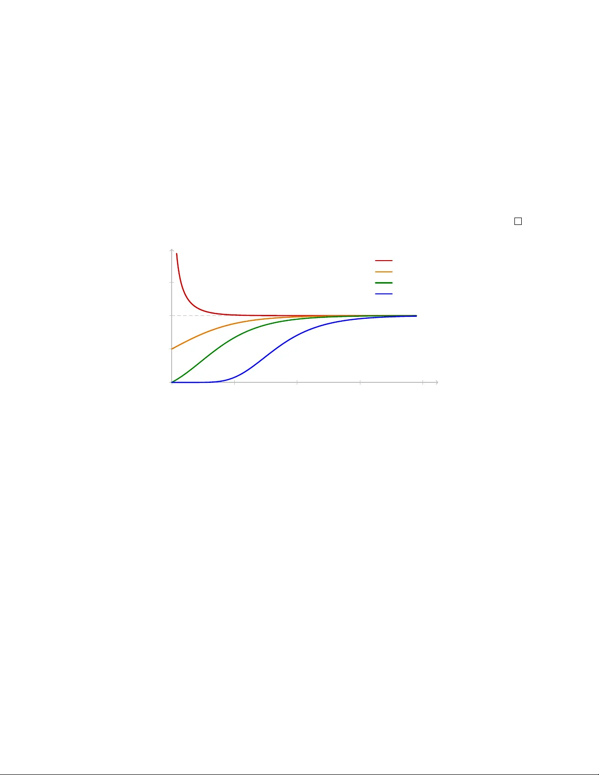
B C T o da c hain I: reﬂection op erator and eigenfunctions N. Belouso v † , S. Derk ac ho v ⋄† , S. Khoroshkin ∗◦† † Beijing Institute of Mathematic al Scienc es and Applic ations, Huair ou district, Beijing, 101408, China ⋄ Steklov Mathematic al Institute, F ontanka 27, St. Petersbur g, 191023, Russia ∗ Dep artment of Mathematics, T e chnion, Haifa, Isr ael ◦ National R ese ar ch University Higher Scho ol of Ec onomics Myasnitskaya 20, Mosc ow, 101000, R ussia Abstract W e obtain Gauss–Given tal integral represen tation for the eigenfunctions of quantum T oda c hain with b oundary in teraction of B C t yp e. F or this we in tro duce reﬂection op erator satisfy- ing reﬂection equation with DST c hain Lax matrices. Besides, w e deﬁne Baxter operators for B C T o da chain, prov e their comm utativity with Hamiltonians and derive the corresp onding Baxter equation. Con ten ts 1 In tro duction 2 1.1 GL T oda chain . . . . . . . . . . . . . . . . . . . . . . . . . . . . . . . . . . . . . 4 1.1.1 Comm uting Hamiltonians . . . . . . . . . . . . . . . . . . . . . . . . . . . 4 1.1.2 Eigenfunctions . . . . . . . . . . . . . . . . . . . . . . . . . . . . . . . . . 5 1.1.3 Baxter op erator . . . . . . . . . . . . . . . . . . . . . . . . . . . . . . . . . 7 1.2 B C T oda chain . . . . . . . . . . . . . . . . . . . . . . . . . . . . . . . . . . . . . 9 1.2.1 Comm uting Hamiltonians . . . . . . . . . . . . . . . . . . . . . . . . . . . 9 1.2.2 Eigenfunctions . . . . . . . . . . . . . . . . . . . . . . . . . . . . . . . . . 10 1.2.3 Baxter op erator . . . . . . . . . . . . . . . . . . . . . . . . . . . . . . . . . 12 1.2.4 Bounds and function spaces . . . . . . . . . . . . . . . . . . . . . . . . . . 13 1.2.5 Relation to XXX spin c hain . . . . . . . . . . . . . . . . . . . . . . . . . . 14 1.2.6 F urther results . . . . . . . . . . . . . . . . . . . . . . . . . . . . . . . . . 14 2 Reﬂection op erator 15 3 Construction of eigenfunctions 20 4 Comm utativit y of Baxter op erators and Hamiltonians 22 5 Baxter equation 23 6 Action of D ( u ) on raising op erator 26 7 Bounds 28 7.1 Lemmas . . . . . . . . . . . . . . . . . . . . . . . . . . . . . . . . . . . . . . . . . 28 7.2 Bounds on eigenfunctions . . . . . . . . . . . . . . . . . . . . . . . . . . . . . . . 34 7.2.1 One particle . . . . . . . . . . . . . . . . . . . . . . . . . . . . . . . . . . . 34 7.2.2 Man y particles . . . . . . . . . . . . . . . . . . . . . . . . . . . . . . . . . 35 7.3 In tertwining relations . . . . . . . . . . . . . . . . . . . . . . . . . . . . . . . . . 39 1 7.4 Mono drom y matrices and op erators . . . . . . . . . . . . . . . . . . . . . . . . . 43 7.5 Baxter op erators . . . . . . . . . . . . . . . . . . . . . . . . . . . . . . . . . . . . 45 A Comm utativit y of Baxter op erators 49 A.1 GL T o da c hain . . . . . . . . . . . . . . . . . . . . . . . . . . . . . . . . . . . . . 49 A.2 B C T o da c hain . . . . . . . . . . . . . . . . . . . . . . . . . . . . . . . . . . . . . 50 B Relation to XXX spin chain 51 B.1 Y ang–Baxter equation . . . . . . . . . . . . . . . . . . . . . . . . . . . . . . . . . 52 B.1.1 Y angian algebra . . . . . . . . . . . . . . . . . . . . . . . . . . . . . . . . 52 B.1.2 Reduction to the DST M -op erators . . . . . . . . . . . . . . . . . . . . . 54 B.1.3 Reduction to the T o da L -op erators . . . . . . . . . . . . . . . . . . . . . . 55 B.2 R -op erators and RLL -relations . . . . . . . . . . . . . . . . . . . . . . . . . . . . 56 B.3 In tertwining operators for the pro ducts of L ± -op erators . . . . . . . . . . . . . . 57 B.3.1 Reduction to the DST intert winers . . . . . . . . . . . . . . . . . . . . . . 59 B.3.2 Reduction to the T o da intert winers . . . . . . . . . . . . . . . . . . . . . . 62 B.4 Reﬂection equation . . . . . . . . . . . . . . . . . . . . . . . . . . . . . . . . . . . 64 1 In tro duction In the present pap er w e study quan tum T o da chain with one-sided b oundary in teraction of B C t yp e. This is a system of n particles with co ordinates x j ∈ R , go v erned by Hamiltonian H B C = − n X j =1 ∂ 2 x j + 2 n − 1 X j =1 e x j − x j +1 + 2 α e − x 1 + β 2 e − 2 x 1 , (1.1) where α, β are parameters. As sho wn in [ Skl2 , I ], this mo del is in tegrable: the ab ov e Hamiltonian b elongs to a c ommuting family of diﬀerential operators H s of the form H s = X 1 ≤ j 1 <... 0 , β > 0 . (1.3) The reason is that already in the simplest case of one particle these conditions ensure that the Hamiltonian ( 1.1 ) has no discrete sp ectra 1 , see [ DL , Theorem 4.3]. The case of B T o da chain is accessed b y taking the limit β → 0. 1 In fact, the same is true if α/β = − 1 / 2, but w e exclude this case to simplify matters. 2 Remark 1. If one restores the Planck constant ℏ in the Hamiltonian, the ﬁrst condition ( 1.3 ) b ecomes α > − ℏ β / 2. The sp ectral problem for one particle  − ∂ 2 x + 2 α e − x + β 2 e − 2 x  Ψ λ ( x ) = λ 2 Ψ λ ( x ) , λ ∈ R , (1.4) has a unique solution deca ying as x → −∞ , whic h is giv en by Whittak er function Ψ λ ( x ) = e x 2 √ 2 β W − α β , − i λ (2 β e − x ) , (1.5) see [ DLMF , Chapter 13 ]. The latter admits the following integral represen tation [ DLMF , (13.16.5) ] Ψ λ ( x ) = e x 2 √ 2 β 2 2i λ (2 β e − x ) − i λ + 1 2 Γ  1 2 + α β − i λ  Z ∞ 1 dt e − β e − x t ( t + 1) − i λ − 1 2 − α β ( t − 1) − i λ − 1 2 + α β . (1.6) Equiv alently , denoting g = 1 2 + α β > 0 (1.7) and c hanging integration v ariable t = e z /β , we ha ve Ψ λ ( x ) = (2 β ) i λ Γ( g − i λ ) Z ∞ ln β dz e i λ ( x − 2 z ) − e z − x (1 + β e − z ) − i λ − g (1 − β e − z ) − i λ + g − 1 . (1.8) The main result of the paper is the generalization of the integral representation ( 1.8 ) to the case of n particles. Denote tuples of n v ariables and sums of their comp onen ts x n = ( x 1 , . . . , x n ) , x n = x 1 + . . . + x n . (1.9) Besides, b y θ ( x ) denote the Hea viside step function θ ( x ) = ( 1 , x ≥ 0 , 0 , x < 0 . (1.10) Theorem 1. The joint eigenfunctions Ψ λ n ( x n ) of the c ommuting Hamiltonians ( 1.2 ) H s Ψ λ n ( x n ) = ( − 1) s X 1 ≤ j 1 <... − g and j, k ∈ { 1 , . . . , n + 1 } . Then the op er ators R j k ( u ) , K j ( v ) , U n,n +1 ( v ) , V n ( v ) act invariantly on the sp ac e E ( R n +1 ) . F urthermor e, for Im v ∈ ( − g , 0) the op er ator Q n ( v ) maps E n ( R n ) to E ( R n ) . With some additional argumen ts this justiﬁes all manipulations with op erators, see Prop o- sitions 3 – 6 and the concluding remarks in Sections 3 – 6 . Combined together they imply the follo wing statement. Corollary 1. Al l r elations with op er ators fr om Se ctions 1.2.2 and 1.2.3 hold on the sp ac es E ( R n +1 ) and E n ( R n ) r esp e ctively (assuming suitable r estrictions on the p ar ameters, as in The o- r em 2 ). Remark 4. The space of exp onen tially temp ered functions E ( R n ) is natural when considering the action of the mono drom y matrix en tries (whic h con tain e ± x j ). It is larger than the Whittak er Sc hw artz space considered by W allach [ W ], whic h is suited to the action of the T o da Hamiltonians rather than the mono drom y matrix. 13 1.2.5 Relation to XXX spin c hain All of the ab o v e statements parallel those obtained recen tly for the op en spin c hain [ ADV2 ]. This can b e explained b y the fact that b oth the DST and T o da chains arise from the XXX spin c hain in a certain limit. In App endix B w e show in detail ho w this limit w orks for diﬀeren t ob jects and equations. First, w e recall the reduction of Lax matrix for XXX spin chain (of spin s ) L ( u ) = u + S S − S + u − S ! = u + z ∂ z + s − ∂ z z 2 ∂ z + 2 sz u − z ∂ z − s ! (1.90) to the Lax matrices for DST and T o da c hains, as explained in [ Skl3 ]. Second, w e consider the reduction of the spin chain R -operator  R 12 ( u 1 | v 1 , v 2 ) Φ  ( z 1 , z 2 ) = 1 Γ( v 1 − u 1 ) Z 1 0 dα α v 1 − u 1 − 1 (1 − α ) u 1 − v 2 × Φ( z 1 , (1 − α ) z 2 + α z 1 ) (1.91) and of the Y ang–Baxter equation it satisﬁes to the T o da chain op erator R 12 ( v ) and the corre- sp onding equation ( 1.27 ), as w ell as to DST c hain R -op erators app earing in Appendix A . A t last, we demonstrate that the spin c hain K -op erator  K ( v , s ) Φ  ( z ) = (2i β ) − 2 v Γ( − 2 v ) ( z + i β ) g + v − s × Z 1 0 dt (1 − t ) − 2 v − 1 t g + v + s − 1  t ( z − i β ) + 2i β  v + s − g Φ( t ( z − i β ) + i β ) (1.92) and the reﬂection equation it satisﬁes can be reduced to the considered previously operator K ( v ) and the corresp onding equation ( 1.64 ). These limiting pro cedures pro vide one more w ay to c hec k the formulas discussed before. 1.2.6 F urther results In the second paper in this series [ BDK ], w e establish several prop erties of the raising and Baxter op erators introduced here, analogous to those for the GL mo del. First, we establish reﬂection symmetry and exc hange relation V n ( λ ) = V n ( − λ ) , V n ( λ ) V n − 1 ( ρ ) = V n ( ρ ) V n − 1 ( λ ) . (1.93) Since eigenfunctions are deﬁned b y the formula Ψ λ n ( x n ) = V n ( λ n ) · · · V 1 ( λ 1 ) · 1 , (1.94) the ab o v e prop erties imply the symmetry in sp ectral parameters under signed permutations Ψ λ 1 ,...,λ n ( x n ) = Ψ ε 1 λ σ (1) ,...,ε n λ σ ( n ) ( x n ) , ε j ∈ { 1 , − 1 } , σ ∈ S n . (1.95) 14 As a result, the sp ectra of Hamiltonians ( 1.63 ) is nondegenerate. F urthermore, this symmetry together with ( 1.78 ) lead to the form ula D ( ± λ j ) Ψ λ n ( x n ) = − β ( g ± i λ j ) Ψ λ 1 ,...,λ j ∓ i ,...,λ n ( x n ) . (1.96) These form ulas are analogues of ( 1.43 ) for the GL mo del. Besides, we pro ve the commutativit y of Baxter op erators and the lo cal relation b etw een Baxter and raising op erators Q n ( λ ) Q n ( ρ ) = Q n ( ρ ) Q n ( λ ) , (1.97) Q n ( λ ) V n ( ρ ) = Γ(i λ − i ρ ) Γ(i λ + i ρ ) V n ( ρ ) Q n − 1 ( λ ) , (1.98) where for n = 1 w e denote Q 0 ( λ ) = (2 β ) − i λ Γ(2i λ ) Γ( g + i λ ) Id . (1.99) F rom the second relation and deﬁnition ( 1.94 ) we deduce that Hamiltonians’ eigenfunctions also diagonalize Baxter op erators Q n ( λ ) Ψ λ n ( x n ) = (2 β ) − i λ Γ(2i λ ) Γ( g + i λ ) n Y j =1 Γ(i λ − i λ j ) Γ(i λ + i λ j ) Ψ λ n ( x n ) . (1.100) This form ula is in accordance with Baxter equation ( 1.86 ). The Baxter op erators’ diagonalization prop erty can b e then used to derive the so-called Mel lin–Barnes r epr esentation for B C T o da eigenfunctions, which generalizes well-kno wn one particle form ula [ DLMF , (13.16.12) ] Ψ λ ( x ) = e x 2 √ 2 β W 1 2 − g , − i λ (2 β e − x ) = e β e − x Z R − i0 dγ 2 π (2 β ) − i γ Γ(i γ − i λ ) Γ(i γ + i λ ) Γ( g + i γ ) e i γ x . (1.101) F or GL T o da c hain Gauss–Given tal and Mellin–Barnes represen tations combined allow one to pro ve orthogonality and completeness of the eigenfunctions [ Sil , K , DKM ], and in the subsequent pap er [ BDK ] w e sho w that the same is true for B C model. Finally , let us remark that the Whittak er function app earing in one particle case ( 1.5 ) also admits series representation [ DLMF , (13.14.33) , (13.14.6) ]. Its generalization to the case of arbitrary num b er of particles is studied in the pap er [ DE ]. In [ BDK ] we present a precise description of suc h a series. 2 Reﬂection op erator In this section w e show ho w to deriv e the following form ula for the reﬂection op erator  K ( v ) φ  ( x ) = (2 β ) i v Γ  1 2 + α β − i v  Z ∞ ln β dy exp  − 2i v y − e y − x   1 + β e − y  − i v − 1 2 − α β ×  1 − β e − y  − i v − 1 2 + α β φ ( − y ) (2.1) 15 from the reﬂection equation with DST Lax matrices K ( v ) M t ( − u − v ) K ( u ) σ 2 M ( u − v ) σ 2 = M ( u − v ) K ( u ) σ 2 M t ( − u − v ) σ 2 K ( v ) . (2.2) Explicitly this equation reads K ( v ) − u − v + i ∂ − e x ∂ e − x i ! − α u − i 2 − β 2  u − i 2  − α ! i e x ∂ − e − x u − v + i ∂ ! = u − v + i ∂ e − x − e x ∂ i ! − α u − i 2 − β 2  u − i 2  − α ! i − e − x e x ∂ − u − v + i ∂ ! K ( v ) , (2.3) where for brevity w e denote ∂ ≡ ∂ x . The deriv ation consist of t wo steps: ﬁrst, w e reduce the matrix equation ab o ve to three relations, tw o of whic h are enough to determine the reﬂection op erator K ( v ) e − x = e x ∂ K ( v ) , (2.4) K ( v )  (i v + ∂ ) e − x − β 2 e x ∂  =  ( − i v − ∂ ) e x ∂ + 2 α + β 2 e − x  K ( v ) . (2.5) The second step is to realize K ( v ) as an integral operator, rewrite these relations as diﬀeren tial equations for its kernel and solve them. After deriv ation we c heck that the solution also satisﬁes the additional third relation giv en by ( 2.9 ). Remark 5. The particular constant behind the in tegral in ( 2.1 ) is chosen to simplify v arious iden tities with reﬂection operator. Besides, the gamma function in denominator suits analytic con tinuation of reﬂection operator, see the end of this section. Reducing matrix equation. The pro duct of matrices from the left hand side of equation ( 2.3 ) can b e represen ted in the follo wing form M t ( − u − v ) K ( u ) σ 2 M ( u − v ) σ 2 = i α ( v − u )  1 0 0 1  + α (2 u − i)  i e x ∂ 0 0  +  u − i 2  ( u + v − i ∂ ) e − x − u 2 + ( v − i ∂ ) 2 − e − 2 x e − x ( u − v + i ∂ ) ! + β 2  u − i 2  i e x ∂ ( e x ∂ ) 2 1 − i e x ∂ ! . Similarly for the pro duct of matrices from the righ t hand side M ( u − v ) K ( u ) σ 2 M t ( − u − v ) σ 2 = i α ( v − u )  1 0 0 1  + α (2 u − i)  0 e − x 0 i  +  u − i 2  ( u − v + i ∂ ) e x ∂ − u 2 + ( v − i ∂ ) 2 − ( e x ∂ ) 2 e x ∂ ( u + v − i ∂ ) ! + β 2  u − i 2  − i e − x e − 2 x 1 i e − x ! . 16 As one can see, the ﬁrst terms with factors ( v − u ) cancel, while all the remaining terms con tain factors ( u − i / 2), which w e remo ve from both sides. After these transformations we arriv e at K ( v ) " 2 α i e x ∂ 0 0 ! + ( u + v − i ∂ ) e − x − u 2 + ( v − i ∂ ) 2 − e − 2 x e − x ( u − v + i ∂ ) ! + β 2 i e x ∂ ( e x ∂ ) 2 1 − i e x ∂ !# = " 2 α 0 e − x 0 i ! + ( u − v + i ∂ ) e x ∂ − u 2 + ( v − i ∂ ) 2 − ( e x ∂ ) 2 e x ∂ ( u + v − i ∂ ) ! + β 2 − i e − x e − 2 x 1 i e − x !# K ( v ) . (2.6) The operator K ( v ) do es not dep end on u , hence, co eﬃcien ts corresp onding to diﬀeren t pow ers of u from both sides should coincide. The equalit y of coeﬃcients b ehind u 2 is trivial, while for u 1 one obtains the relation ( 2.4 ) K ( v ) e − x = e x ∂ K ( v ) . (2.7) It remains to consider the matrix relation ( 2.6 ) at u = 0 K ( v ) " 2 α i e x ∂ 0 0 ! + ( v − i ∂ ) e − x ( v − i ∂ ) 2 − e − 2 x e − x ( − v + i ∂ ) ! + β 2 i e x ∂ ( e x ∂ ) 2 1 − i e x ∂ !# = " 2 α 0 e − x 0 i ! + ( − v + i ∂ ) e x ∂ ( v − i ∂ ) 2 − ( e x ∂ ) 2 e x ∂ ( v − i ∂ ) ! + β 2 − i e − x e − 2 x 1 i e − x !# K ( v ) . (2.8) The equalit y b et ween (2 , 1) matrix elemen ts K ( v ) e − 2 x = ( e x ∂ ) 2 K ( v ) is evident consequence of ( 2.7 ). The remaining relations corresp onding to (1 , 1), (2 , 2) and (1 , 2) matrix elemen ts are as follows K ( v )  ( v − i ∂ ) e − x + 2i α + i β 2 e x ∂  =  ( − v + i ∂ ) e x ∂ − i β 2 e − x  K ( v ) , K ( v )  e − x ( − v + i ∂ ) − i β 2 e x ∂  =  e x ∂ ( v − i ∂ ) + 2i α + i β 2 e − x  K ( v ) , K ( v )  ( v − i ∂ ) 2 + 2 α e x ∂ + β 2 ( e x ∂ ) 2  =  ( v − i ∂ ) 2 + 2 α e − x + β 2 e − 2 x  K ( v ) . (2.9) Notice that the ﬁrst equation coincides with the announced relation ( 2.5 ). The second equation is equiv alent to the ﬁrst one due to ( 2.7 ): one just needs to rewrite the ﬁrst terms from b oth sides e − x ( − v + i ∂ ) = ( − v + i ∂ ) e − x + i e − x , e x ∂ ( v − i ∂ ) = ( v − i ∂ ) e x ∂ + i e x ∂ . (2.10) Th us, we reduced the initial matrix equation to three relations. Two of them are enough to determine the explicit form of reﬂection op erator, while the third one ( 2.9 ) can b e c heck ed at the end. 17 Solving k ey relations. T o solve tw o relations K ( v ) e − x = e x ∂ K ( v ) , K ( v )  (i v + ∂ ) e − x − β 2 e x ∂  =  ( − i v − ∂ ) e x ∂ + 2 α + β 2 e − x  K ( v ) (2.11) w e realize K ( v ) as an in tegral op erator acting on function φ ( x ) by the form ula  K ( v ) φ  ( x ) = Z C dy K ( x, y ) φ ( − y ) . (2.12) Moreo ver, w e assume that the con tour C and function φ ( x ) are suc h that b oundary terms from in tegration by parts v anish  K ( v ) ∂ φ  ( x ) = − Z C dy K ( x, y ) ∂ y φ ( − y ) = Z C dy  ∂ y K ( x, y )  φ ( − y ) . (2.13) Then the relations ( 2.11 ) can b e rewritten as equations for the k ernel ∂ x K ( x, y ) = e y − x K ( x, y ) , (2.14) ∂ y K ( x, y ) =  1 − e y − x + 2 α e − y − 1 − 2i v 1 − β 2 e − 2 y  K ( x, y ) . (2.15) The solution of these diﬀeren tial equations has the form K ( x, y ) = A exp  − 2i v y − e y − x   1 + β e − y  − i v − 1 2 − α β  1 − β e − y  − i v − 1 2 + α β (2.16) where A is arbitrary constan t. This coincides with the stated expression ( 2.1 ). In the same wa y , integrating b y parts one rewrites the third relation ( 2.9 ) as the equation on the k ernel  ( v − i ∂ y ) 2 − ( v − i ∂ x ) 2 + 2 α  ∂ y e − y − e − x  + β 2  ( ∂ y e − y ) 2 − e − 2 x   K ( x, y ) = 0 . (2.17) It is straigh tforward to c hec k that the solution ( 2.16 ) satisﬁes this equation as well. No w let us commen t on the choice of in tegration contour and space of functions in ( 2.12 ). The k ernel K ( x, y ) is fastly decreasing as y → ∞ for any v ∈ C . Besides, it is in tegrable near y = ln β under assumption Re  − i v − 1 2 + α β  > − 1 ⇔ Im v > − 1 2 − α β . (2.18) Th us, under this condition the action of reﬂection operator ( 2.12 ) with integration along the real line C = (ln β , ∞ ) is well deﬁned on con tinuous functions φ ( x ) that don’t grow too rapidly as x → −∞ . Ho wev er, to hav e v anishing b oundary terms after integrating by parts ( 2.13 ) one needs additional constrain ts on φ ( x ) and the stronger assumption Re  − i v − 1 2 + α β  > 0 ⇔ Im v > 1 2 − α β , (2.19) 18 whic h guarantees that lim y → ln β + (1 − β e − y ) − i v − 1 2 + α β = 0 . (2.20) F urthermore, for the third relation ( 2.9 ) we need to integrate b y parts t w o times, whic h makes the necessary assumption on v ev en stronger: Im v > 3 / 2 − α/β . The crux is that in analysis of T o da eigenfunctions w e need reﬂection equation with the w eakest of all assumptions Im v > − 1 / 2 − α/β . This leads to the following strategy: (1) ﬁnd nice enough space of functions φ ( x ), such that [ K ( v ) φ ]( x ) and its deriv atives with resp ect to x are analytic in v under assumption Im v > − 1 / 2 − α/β ; (2) under stronger assumption Im v > 3 / 2 − α/β prov e relations ( 2.9 ), ( 2.11 ) (and consequently , reﬂection equation ( 2.2 )) using in tegration by parts; (3) analytically contin ue these relations to the domain Im v > − 1 / 2 − α/β at the end. The details are giv en in Section 7.3 , and here we only state the result. The suitable space, whic h is denoted b y E , consists of exp onential ly temp er e d smooth functions φ ( x ) ∈ C ∞ ( R ), that is for an y k ∈ N 0 there exist a, b ≥ 0 such that   φ ( k ) ( x )   ≤ a e b | x | . (2.21) On such space the reﬂection op erator K ( v ) is well deﬁned and the reﬂection equation ( 2.2 ) holds under assumption Im v > − 1 / 2 − α /β . This concludes the pro of of the form ula ( 2.1 ). Analytic contin uation. Let us men tion that the action of reﬂection op erator K ( v ) can be analytically con tinued to the whole complex plane v ∈ C , if we consider functions φ ( x ) that are analytic and don’t gro w to o rapidly in some strip near real line. y ln β H Figure 1: Hank el contour and branc h cut The k ernel K ( x, y ) ( 2.16 ) has the branch cut along the in terv al [ln β , ∞ ). Hence, in the realization of reﬂection op erator ( 2.12 ) we can alternativ ely c ho ose Hankel contour C = H , see Figure 1 . If one also c ho oses the diﬀeren t constant behind the integral, namely  K an ( v ) φ  ( x ) = − (2 β ) i v Γ  1 2 − α β + i v  2 π i Z H dy exp  − 2i v y − e y − x   1 + β e − y  − i v − 1 2 − α β ×  1 − β e − y  − i v − 1 2 + α β φ ( − y ) , (2.22) 19 then the corresp onding expression represen ts analytic contin uation of the ﬁrst formula for the reﬂection op erator ( 2.1 ). Indeed, assuming Im v > − 1 / 2 − α/β we can standardly pass from the Hank el contour to the branc h cut Z H dy K ( x, y ) φ ( − y ) = lim ε → 0 + Z ∞ ln β dy  K ( x, y − i ε ) − K ( x, y + i ε )  φ ( − y ) = 2i sin  π  − i v − 1 2 + α β  Z ∞ ln β dy K ( x, y ) φ ( − y ) . (2.23) F rom this using the well kno wn formula sin  π  − i v − 1 2 + α β  = − π Γ  1 2 + α β − i v  Γ  1 2 − α β + i v  (2.24) w e deduce that K an ( v ) = K ( v ). 3 Construction of eigenfunctions By Prop osition 6 pro v en in Section 7.4 , the mono drom y op erator U n 0 ( v ) = R n 0 ( v ) · · · R 10 ( v ) K 0 ( v ) R ∗ 10 ( v ) · · · R ∗ n 0 ( v ) (3.1) satisﬁes reﬂection equation U n 0 ( v ) M t 0 ( − u − v ) T n ( u ) σ 2 M 0 ( u − v ) σ 2 = M 0 ( u − v ) T n ( u ) σ 2 M t 0 ( − u − v ) σ 2 U n 0 ( v ) . (3.2) In the simplest case n = 0 w e ha ve U 00 ( v ) = K 0 ( v ) , T 0 ( u ) = K ( u ) . (3.3) Explicitly , acting on function φ ( x n , x 0 ) the mono drom y op erator is giv en b y the formula  U n 0 ( v ) φ  ( x n ) = Z R n d y n U v ( x n | y n ) φ ( y n , − x n ) (3.4) with the k ernel U v ( x n | y n ) = (2 β ) i v Γ( g − i v ) Z R n +1 d z n +1 exp  i v  x n + y n − 2 z n +1  − n X j =1 ( e z j − x j + e z j − y j + e x j − z j +1 + e y j − z j +1 ) − e z n +1 − x 0  ×  1 + β e − z 1  − i v − g  1 − β e − z 1  − i v + g − 1 θ ( z 1 − ln β ) . (3.5) The raising operator V n ( λ ) maps functions of n − 1 co ordinates φ ( x n − 1 ) to functions of n co or- dinates. It is deﬁned as a restriction of mono drom y op erator V n ( λ ) = e i λx n U n − 1 ,n ( λ )   φ ( x n − 1 ) . (3.6) 20 In this section w e demonstrate that eigenfunctions of B C T o da c hain B n ( u ) Ψ λ n ( x n ) =  u − i 2  n Y j =1 ( λ 2 j − u 2 ) Ψ λ n ( x n ) (3.7) can b e constructed using raising operators Ψ λ n ( x n ) = V n ( λ n ) · · · V 1 ( λ 1 ) · 1 . (3.8) F or this we sho w that raising op erator satisﬁes the following relation with B -operator B n ( u ) V n ( λ ) = ( λ 2 − u 2 ) V n ( λ ) B n − 1 ( u ) . (3.9) Note that b y deﬁnition B 0 = ( u − i / 2). Th us, the latter relation applied to the function ( 3.8 ) leads to the form ula ( 3.7 ). T o prov e ( 3.9 ) we write DST matrices in the relation ( 3.2 ) explicitly U n − 1 ,n ( v ) − u − v + i ∂ n − e x n ∂ n e − x n i ! T n − 1 ( u ) i e x n ∂ n − e − x n u − v + i ∂ n ! = u − v + i ∂ n e − x n − e x n ∂ n i ! T n − 1 ( u ) i − e − x n e x n ∂ n − u − v + i ∂ n ! U n − 1 ,n ( v ) . (3.10) First, let us extract the equality of (1 , 2) matrix elemen ts. That is consider the ﬁrst ro w from the most left matrix and the second column from the most righ t matrix U n − 1 ,n ( v )  − u − v + i ∂ n − e x n ∂ n  T n − 1 ( u ) e x n ∂ n u − v + i ∂ n ! =  u − v + i ∂ n e − x n  T n − 1 ( u ) − e − x n − u − v + i ∂ n ! U n − 1 ,n ( v ) . (3.11) Next transform the ro w and column in the right hand side  u − v + i ∂ n e − x n  = e − i v x n  u + i ∂ n e − x n  e i v x n , (3.12) − e − x n − u − v + i ∂ n ! = e − i v x n − e − x n − u + i ∂ n ! e i v x n . (3.13) Note that the transformed row coincides with the ﬁrst row of the matrix L n ( u ), while transformed column coincides with the second column of the matrix σ 2 L t n ( − u ) σ 2 L n ( u ) = u + i ∂ n e − x n − e x n 0 ! , σ 2 L t n ( − u ) σ 2 = 0 − e − x n e x n − u + i ∂ n ! . (3.14) Besides, recall that b y deﬁnition T n ( u ) = L n ( u ) T n − 1 ( u ) σ 2 L t n ( − u ) σ 2 = A n ( u ) B n ( u ) C n ( u ) D n ( u ) ! . (3.15) 21 Hence, after transformations in the righ t hand side of the form ula ( 3.11 ) w e obtain the op era- tor B n ( u ) U n − 1 ,n ( v )  − u − v + i ∂ n − e x n ∂ n  T n − 1 ( u ) e x n ∂ n u − v + i ∂ n ! = e − i v x n B n ( u ) e i v x n U n − 1 ,n ( v ) . (3.16) If w e apply this op erator identit y to the function whic h does not depend on x n , then deriv a- tiv es ∂ n from the left disapp ear U n − 1 ,n ( v )  − u − v 0  A n − 1 ( u ) B n − 1 ( u ) C n − 1 ( u ) D n − 1 ( u ) ! 0 u − v ! φ ( x n − 1 ) = e − i v x n B n ( u ) e i v x n U n − 1 ,n ( v ) φ ( x n − 1 ) . (3.17) Simplifying the left hand side w e arrive at the form ula ( v 2 − u 2 ) e i v x n U n − 1 ,n ( v ) B n − 1 ( u ) φ ( x n − 1 ) = B n ( u ) e i v x n U n − 1 ,n ( v ) φ ( x n − 1 ) , (3.18) whic h coincides with the stated relation ( 3.9 ). Finally , let us remark that the initial matrix relation ( 3.10 ) holds on the space of exp o- nen tially tempered smooth functions E ( R n ), see Proposition 6 . Hence, the same is true for the in tertwining relation ( 3.9 ). In Section 7.2 w e pro ve that the in tegral representation ( 3.8 ) is abso- lutely con vergen t and deriv e estimate for it (Proposition 1 ). This estimate, in particular, implies that the eigenfunctions b elong to the space E ( R n ) (Corollary 7 ), whic h justiﬁes the construction ab o v e. 4 Comm utativit y of Baxter op erators and Hamiltonians Baxter op erator is related to the monodromy operator ( 3.1 ) through the restriction and limit Q n ( λ ) = lim x 0 →∞ U n 0 ( λ )   φ ( x n ) . (4.1) Explicitly , it is given b y the integral operator  Q n ( λ ) φ  ( x n ) = Z R n d y n Q λ ( x n | y n ) φ ( y n ) (4.2) with the k ernel Q λ ( x n | y n ) = (2 β ) i λ Γ( g − i λ ) Z R n +1 d z n +1 exp  i λ  x n + y n − 2 z n +1  − n X j =1 ( e z j − x j + e z j − y j + e x j − z j +1 + e y j − z j +1 )  ×  1 + β e − z 1  − i λ − g  1 − β e − z 1  − i λ + g − 1 θ ( z 1 − ln β ) , (4.3) 22 whic h is con vergen t under assumption Im λ ∈ ( − g , 0). The explicit expression for the k ernel follo ws from the formula ( 3.5 ). The interc hange of limit and integration is justiﬁed for a suitable space of functions φ ( x n ), see Corollary 5 in Section 7.5 . In this section w e prov e that Baxter op erators comm ute with Hamiltonians B n ( u ) Q n ( λ ) = Q n ( λ ) B n ( u ) . (4.4) First, recall the in tertwining relation for the monodromy operator ( 3.2 ) U n 0 ( v ) − u − v + i ∂ 0 − e x 0 ∂ 0 e − x 0 i ! T n ( u ) i e x 0 ∂ 0 − e − x 0 u − v + i ∂ 0 ! = u − v + i ∂ 0 e − x 0 − e x 0 ∂ 0 i ! T n ( u ) i − e − x 0 e x 0 ∂ 0 − u − v + i ∂ 0 ! U n 0 ( v ) . (4.5) Consider the equality of (1 , 2) elemen ts and act from b oth sides on function φ ( x n ), so that the deriv atives ∂ 0 from the left disapp ear ( − u − v )( u − v ) U n 0 ( v ) B n ( u ) φ ( x n ) =  u − v + i ∂ 0 e − x 0  A n ( u ) B n ( u ) C n ( u ) D n ( u ) ! − e − x 0 − u − v + i ∂ 0 ! U n 0 ( v ) φ ( x n ) . (4.6) Next we tak e the limit x 0 → ∞ . The exp onen ts e − x 0 from the right v anish. Besides, the explicit form ula for the kernel of monodromy operator ( 3.5 ) suggests the equality lim x 0 →∞ ∂ 0 U n 0 ( v ) φ ( x n ) = 0 . (4.7) It is pro v en in Section 7.5 for a suitable space of functions φ ( x n ), see Corollary 5 . Thus, in the limit x 0 → ∞ it is possible to remov e e − x 0 and ∂ 0 from the righ t hand side of ( 4.6 ), so that this relation is reduced to the needed form lim x 0 →∞ U n 0 ( v ) B n ( u ) φ ( x n ) = B n ( u ) lim x 0 →∞ U n 0 ( v ) φ ( x n ) . (4.8) The tec hnical details ab out the spaces of functions, on whic h all ab o ve relations hold are giv en in Section 7.5 . Namely , by Corollary 5 Baxter op erators are w ell deﬁned on the space of exp onen tially temp ered smo oth functions with at most p olynomial growth as x n → ∞ , whic h w e denote b y E n ( R n ). Moreov er, Baxter op erator maps this space to E ( R n ), while the op erator B n ( u ) acts in v arian tly on it, see Corollary 6 . 5 Baxter equation In this section w e derive the Baxter equation Q n ( u ) B n ( u ) = − β ( g + i u ) 2 u Q n ( u − i) . (5.1) The deriv ation consists of t w o parts. First, we rewrite some kno wn lo cal relations with R - and K -op erators in a suitable form. Second, we use them to perform reduction of a certain global relation with mono drom y op erator and monodromy matrix. 23 Rewriting lo cal relations. T o b egin, w e rewrite in tertwining relation ( 1.27 ) R 12 ( v ) L 1 ( u ) M 2 ( u − v ) = M 2 ( u − v ) L 1 ( u ) R 12 ( v ) (5.2) in an equiv alent form U − 1 2 R 12 ( v ) L 1 ( u ) U 2 = V 2 ( u − v ) L 1 ( u ) R 12 ( v ) V − 1 2 ( u − v ) (5.3) using factorized expression for the matrix M ( λ ) M ( λ ) = λ + i ∂ x e − x − e x ∂ x i ! = U V ( λ ) , (5.4) where U = 1 − i e − x 0 1 ! , V ( λ ) = λ 0 − e x ∂ x i ! . (5.5) Next with the help of explicit expression for the op erator R 12 ( v ) ( 1.28 ) w e rewrite the rela- tion ( 5.3 ) as follo ws U − 1 2 R 12 ( v ) L 1 ( u ) U 2 = ( u − v ) R 12 ( v ) − i R 12 ( v − i) − i( u − v ) e − x 1 R 12 ( v ) − e x 1 R 12 ( v + i) i e x 21 ∂ 2 R 12 ( v ) ! , (5.6) so that at the p oin t v = u one obtains U − 1 2 R 12 ( u ) L 1 ( u ) U 2 = − i R 12 ( u − i) 0 − e x 1 R 12 ( u + i) i e x 21 ∂ 2 R 12 ( u ) ! . (5.7) Here for brevit y we denote x 21 ≡ x 2 − x 1 . Similarly for the op erator R ∗ 12 ( u ) ( 1.69 ) w e hav e e U − 1 2 R ∗ 12 ( u ) e L 1 ( u ) e U 2 = − i e x 2 + x 1 ∂ 2 R ∗ 12 ( u ) − e − x 1 R ∗ 12 ( u + i) 0 i R ∗ 12 ( u − i) ! (5.8) where e U = σ 2 U σ 2 , e L ( u ) = σ 2 L t ( − u ) σ 2 . (5.9) The same factorization ( 5.4 ) can b e used to transform the reﬂection equation ( 2.2 ) K ( v ) M t ( − u − v ) K ( u ) σ 2 M ( u − v ) σ 2 = M ( u − v ) K ( u ) σ 2 M t ( − u − v ) σ 2 K ( v ) (5.10) to the form U − 1 K ( v ) M t ( − u − v ) K ( u ) e U = V ( u − v ) K ( u ) σ 2 M t ( − u − v ) σ 2 K ( v ) σ 2 V − 1 ( u − v ) σ 2 . (5.11) Notice that in the righ t hand side we ha v e singularity at v = u σ 2 V − 1 ( u − v ) σ 2 = − i i u − v e x ∂ x 0 1 u − v ! . (5.12) 24 The last relation can b e rewritten as U − 1 K ( v ) M t ( − u − v ) K ( u ) e U = 1 0 − e x ∂ x u − v i u − v ! K ( u ) ( u − v ) K ( v ) −K ( v ) e x ∂ x − e − x K ( v ) − i( u − v ) e x ∂ x K ( v ) i  ∂ x K ( v ) + K ( v ) ∂ x  − ( u + v ) K ( v ) ! . (5.13) Consider only the ﬁrst ro w of this matrix equality and put v = u  1 0  U − 1 K ( u ) M t ( − 2 u ) K ( u ) e U =  1 0  K ( u ) 0 −K ( u ) e x ∂ x − e − x K ( u ) 0 i  ∂ x K ( u ) + K ( u ) ∂ x  − 2 u K ( u ) ! . (5.14) Then using explicit form ula for the reﬂection op erator ( 2.1 ) we can rewrite the righ t hand side in a simpler form  1 0  U − 1 K ( u ) M t ( − 2 u ) K ( u ) e U = β ( g + i u ) K ( u − i)  0 1  . (5.15) The deriv ation of the Baxter equation is based on the obtained lo cal relations ( 5.7 ), ( 5.8 ) and ( 5.15 ). Reducing global relation. Recall deﬁnitions of the mono drom y op erator and matrix U n 0 ( v ) = R n 0 ( v ) · · · R 10 ( v ) K 0 ( v ) R ∗ 10 ( v ) · · · R ∗ n 0 ( v ) , T n ( u ) = L n ( u ) · · · L 1 ( u ) K ( u ) e L 1 ( u ) · · · e L n ( u ) . (5.16) Using them together with the comm utation relation ( 1.68 ) R ∗ 12 ( v ) M t 2 ( − u − v ) L 1 ( u ) = L 1 ( u ) M t 2 ( − u − v ) R ∗ 12 ( v ) (5.17) w e arrive at the follo wing global relation U n 0 ( v ) M t 0 ( − u − v ) T n ( u ) = R n 0 ( v ) L n ( u ) · · · R 10 ( v ) L 1 ( u ) × K 0 ( v ) M t 0 ( − u − v ) K ( u ) R ∗ 10 ( v ) e L 1 ( u ) · · · R ∗ n 0 ( v ) e L n ( u ) . (5.18) No w consider (1 , 2) element of the matrix from the left, put v = u and p erform corresponding reductions to obtain Baxter op erator ( 4.1 ) lim x 0 →∞ U n 0 ( u )  − 2 u + i ∂ x 0 − e x 0 ∂ x 0  B n ( u ) D n ( u ) ! φ ( x n ) = − 2 u Q n ( u ) B n ( u ) φ ( x n ) . (5.19) The last pro duct is as needed in the Baxter equation ( 5.1 ) Next step is to extract the same matrix elemen t from the right hand side ( 5.18 ), but b efore let us divide it in to three parts h R n 0 ( v ) L n ( u ) · · · R 10 ( v ) L 1 ( u ) U 0 i × h U − 1 0 K 0 ( v ) M t 0 ( − u − v ) K ( u ) e U 0 i h e U − 1 0 R ∗ 10 ( v ) e L 1 ( u ) · · · R ∗ n 0 ( v ) e L n ( u ) i , (5.20) 25 and transform these parts separately using kno wn lo cal relations. First, using lo cal relation ( 5.7 ) w e rewrite the ﬁrst pro duct in square brac k ets U 0 U − 1 0 R n 0 ( u ) L n ( u ) · · · R 10 ( u ) L 1 ( u ) U 0 = 1 − i e − x 0 0 1 ! × − i R n 0 ( u − i) 0 − e x n R n 0 ( u + i) i e x 0 n ∂ 0 R n 0 ( u ) ! · · · − i R 10 ( u − i) 0 − e x 1 R 10 ( u + i) i e x 01 ∂ 0 R 10 ( u ) ! . (5.21) In the limit x 0 → ∞ the exponent e − x 0 v anishes, so that one obtains the following ﬁrst ro w lim x 0 →∞  1 0  R n 0 ( u ) L n ( u ) · · · R 10 ( u ) L 1 ( u ) U 0 = lim x 0 →∞ ( − i) n R n 0 ( u − i) · · · R 10 ( u − i)  1 0  . (5.22) Since the result is prop ortional to the vector (1 0), in the second pro duct in square brac k- ets ( 5.20 ) w e also need to extract only the ﬁrst row. This allows us to use local relation ( 5.15 )  1 0  U − 1 0 K 0 ( u ) M t 0 ( − 2 u ) K ( u ) e U 0 = β ( g + i u ) K 0 ( u − i)  0 1  . (5.23) Again, since the result is prop ortional to the v ector (0 1), in the last pro duct in square brac k- ets ( 5.20 ) w e only need (2 , 2) entry . Using the lo cal relation ( 5.8 ) w e obtain  0 1  e U − 1 0 R ∗ 10 ( u ) e L 1 ( u ) · · · R ∗ n 0 ( u ) e L n ( u ) e U 0 e U − 1 0  0 1  = i n R ∗ 10 ( u − i) · · · R ∗ n 0 ( u − i) . (5.24) Collecting ev erything together we arriv e at the follo wing relation − 2 u Q n ( u ) B n ( u ) φ ( x n ) = β ( g + i u ) lim x 0 →∞ R n 0 ( u − i) · · · R 10 ( u − i) K 0 ( u − i) R ∗ 10 ( u − i) · · · R ∗ n 0 ( u − i) φ ( x n ) , (5.25) whic h is equiv alen t to the announced Baxter equation ( 5.1 ). In full analogy with the previous section, all relations used here hold on the space E n ( R n ). The only subtle p oin t is that the sp ectral parameter of the Baxter op erator Q n ( u ) should satisfy Im u ∈ ( − g , 0), see Corollary 5 . Hence, the app earance of Q n ( u − i) on the righ t requires a stronger condition Im u ∈ (1 − g , 0), whic h is non-empty only if g > 1. 6 Action of D ( u ) on raising op erator With a minor mo diﬁcation of the deriv ation from the previous section, w e can compute the action of D n ( u ) on the raising op erator D n ( u ) V n ( u ) = − β ( g + i u ) V n ( u − i) . (6.1) W e start with the equality ( 3.2 ) M n ( u − v ) T n − 1 ( u ) σ 2 M t n ( − u − v ) σ 2 U n − 1 ,n ( v ) = U n − 1 ,n ( v ) M t n ( − u − v ) T n − 1 ( u ) σ 2 M n ( u − v ) σ 2 . (6.2) 26 Next we insert deﬁnitions of mono drom y op erator and monodromy matrix ( 5.16 ) from the right and use in tertwining relation ( 5.17 ) to obtain M n ( u − v ) T n − 1 ( u ) σ 2 M t n ( − u − v ) σ 2 U n − 1 ,n ( v ) = R n − 1 ,n ( v ) L n − 1 ( u ) · · · R 1 n ( v ) L 1 ( u ) K n ( v ) M t n ( − u − v ) K ( u ) × R ∗ 1 n ( v ) e L 1 ( u ) · · · R ∗ n − 1 ,n ( v ) e L n − 1 ( u ) σ 2 M n ( u − v ) σ 2 . (6.3) Multiplying b oth sides b y the v ector e i v x n  − e x n 0  M − 1 n ( u − v ) = e i v x n i( u − v )  − i e x n 1  (6.4) w e arrive at the equalit y  − e x n 0  T n − 1 ( u ) e i v x n σ 2 M t n ( − u − v ) σ 2 e − i v x n e i v x n U n − 1 ,n ( v ) = e i v x n  − e x n 0  M − 1 n ( u − v ) R n − 1 ,n ( v ) L n − 1 ( u ) · · · R 1 n ( v ) L 1 ( u ) K n ( v ) M t n ( − u − v ) K ( u ) × R ∗ 1 n ( v ) e L 1 ( u ) · · · R ∗ n − 1 ,n ( v ) e L n − 1 ( u ) σ 2 M n ( u − v ) σ 2 , (6.5) or writing all matrices explicitly  − e x n 0  T n − 1 ( u ) i − e − x n e x n ( ∂ n − i v ) − u + i ∂ n ! e i v x n U n − 1 ,n ( v ) = e i v x n i( u − v )  − i e x n 1  R n − 1 ,n ( v ) L n − 1 ( u ) · · · R 1 n ( v ) L 1 ( u ) K n ( v ) M t n ( − u − v ) K ( u ) × R ∗ 1 n ( v ) e L 1 ( u ) · · · R ∗ n − 1 ,n ( v ) e L n − 1 ( u ) i e x n ∂ n − e x n u − v + i ∂ n ! . (6.6) No w we multiply b oth sides from the right by the vector (0 1) t and act on function φ ( x n − 1 ), so that the deriv atives ∂ n from the righ t disapp ear  − e x n 0  T n − 1 ( u ) − e − x n − u + i ∂ n ! e i v x n U n − 1 ,n ( v ) φ ( x n − 1 ) = − i e i v x n  − i e x n 1  R n − 1 ,n ( v ) L n − 1 ( u ) · · · R 1 n ( v ) L 1 ( u ) K n ( v ) M t n ( − u − v ) K ( u ) × R ∗ 1 n ( v ) e L 1 ( u ) · · · R ∗ n − 1 ,n ( v ) e L n − 1 ( u )  0 1  φ ( x n − 1 ) . (6.7) By deﬁnitions, D n ( u ) =  − e x n 0  T n − 1 ( u ) − e − x n − u + i ∂ n ! , V n ( v ) = e i v x n U n − 1 ,n ( v )   φ ( x n − 1 ) , (6.8) 27 so the left hand side of the last expression at the p oin t v = u is as desired ( 6.1 ). Besides, in the righ t hand side the same mechanism applies as in the deriv ation of the Baxter equation. First, putting v = u due to ( 5.7 ) w e hav e  − i e x n 1  R n − 1 ,n ( u ) L n − 1 ( u ) · · · R 1 n ( u ) L 1 ( u ) U n =  − i e x n 1  1 − i e − x n 0 1 ! × − i R n − 1 ,n ( u − i) 0 − e x n − 1 R n − 1 ,n ( u + i) i e x n − 1 n ∂ 0 R n − 1 ,n ( u ) ! · · · − i R 1 n ( u − i) 0 − e x 1 R 1 n ( u + i) i e x n 1 ∂ n R 1 n ( u ) ! = ( − i) n e x n R n − 1 ,n ( u − i) · · · R 1 n ( u − i)  1 0  . (6.9) This leads to the selection of the ﬁrst row in the next pro duct containing reﬂection op erator, whic h allows to put v = u and use relation ( 5.15 )  1 0  U − 1 n K n ( u ) M t n ( − 2 u ) K ( u ) e U n = β ( g + i u ) K n ( u − i)  0 1  . (6.10) Consequen tly , from the pro duct with R ∗ -op erators in the last line ( 6.7 ) we only need (2 , 2) elemen t. Due to ( 5.8 ) it equals  0 1  e U − 1 n R ∗ 1 n ( u ) e L 1 ( u ) · · · R ∗ n − 1 ,n ( u ) e L n − 1 ( u ) e U n − 1 e U − 1 n − 1  0 1  = i n − 1 R ∗ 1 n ( u − i) · · · R ∗ n − 1 ,n ( u − i) . (6.11) Collecting ev erything together we obtain the follo wing relation D n ( u ) V n ( u ) φ ( x n − 1 ) = − β ( g + i u ) e i( u − i) x n R n − 1 ,n ( u − i) · · · R 1 n ( u − i) K n ( u − i) × R ∗ 1 n ( u − i) · · · R ∗ n − 1 ,n ( u − i) φ ( x n − 1 ) , (6.12) whic h coincides with the desired formula ( 6.1 ). A t last, let us remark that the initial equality and all used in tertwining relations hold on the space E ( R n ) assuming Im u > 1 − g , see Sections 7.3 – 7.4 . 7 Bounds In this section we deriv e b ounds on eigenfunctions and study spaces of functions, on which the op erators considered in the paper are well deﬁned and relations betw een them hold true. 7.1 Lemmas The idea b ehind the follo wing tw o lemmas (whic h w e b orro w from [ BC , Section 4.1.1]) is that double exp onen t e − e y is a smo oth v ersion of step function θ ( − y ), see Figure 2 . Lemma 1. L et s > 0 , κ ∈ R and x ≥ 0 . Then Z ∞ 0 dy y s − 1 e κy − e y + x ≤ C ( s, κ ) e − e x , (7.1) and c onver genc e of this inte gr al is uniform in x ≥ 0 . 28 − 4 − 2 2 4 0 . 5 1 y Figure 2: Graph of e − e y Pr o of. The b ound can b e equiv alently written as Z ∞ 0 dy y s − 1 e κy − e x ( e y − 1) ≤ C ( s, κ ) . (7.2) Since e x ≥ 1 and e y − 1 ≥ y 2 / 2 for y ≥ 0, we ha ve Z ∞ 0 dy y s − 1 e κy − e x ( e y − 1) ≤ Z ∞ 0 dy y s − 1 e κy − 1 2 y 2 . (7.3) The last integral is conv ergent due to assumption s > 0. Besides, con v ergence of initial in tegral is uniform in x due to inequalit y e − e y + x ≤ e − e y . Lemma 2. L et m ∈ N 0 , κ ≥ 0 and x 1 , x 2 ∈ R . Then Z R dy | y | m exp  κ ( x 1 − y ) − e x 1 − y − e y − x 2  ≤ P ( | x 1 | , | x 2 | ) exp  κ x 1 − x 2 2 − e x 1 − x 2 2  θ ( x 1 − x 2 )  , (7.4) wher e P ( | x 1 | , | x 2 | ) ≡ P ( | x 1 | , | x 2 | ; m, κ ) is p olynomial in | x j | . Conver genc e of this inte gr al is uniform in x 1 , x 2 fr om c omp act subsets of R . Pr o of. First, consider the case x 1 ≤ x 2 . W e need to prov e that the integral is b ounded b y p olynomial Z R dy | y | m e κ ( x 1 − y ) − e x 1 − y − e y − x 2 ≤ P ( | x 1 | , | x 2 | ) . (7.5) Let us divide it in to three parts Z R dy = Z x 1 −∞ dy + Z x 2 x 1 dy + Z ∞ x 2 dy , (7.6) 29 whic h w e estimate separately . In the ﬁrst term use inequalit y e − e y − x 2 ≤ 1 and c hange in tegration v ariable to z = x 1 − y Z x 1 −∞ dy | y | m e κ ( x 1 − y ) − e x 1 − y − e y − x 2 ≤ Z x 1 −∞ dy | y | m e κ ( x 1 − y ) − e x 1 − y = Z ∞ 0 dz | x 1 − z | m e κz − e z ≤ Z ∞ 0 dz ( | x 1 | + z ) m e κz − e z . (7.7) The last in tegral is polynomial in | x 1 | , since expanding brac kets w e obtain integrals of the t yp e Z ∞ 0 dz z ℓ e κz − e z < ∞ . (7.8) Besides, its con vergence is clearly uniform in x 1 , x 2 from compact subsets of R . The third integral from ( 7.6 ) is b ounded b y p olynomial in | x 2 | in similar wa y (notice that e κ ( x 1 − y ) ≤ e κ ( x 1 − x 2 ) ≤ 1 for y ≥ x 2 ) and it also conv erges uniformly in x 1 , x 2 . At last, the second in tegral from ( 7.6 ) can b e estimated in the follo wing wa y Z x 2 x 1 dy | y | m e κ ( x 1 − y ) − e x 1 − y − e y − x 2 ≤ Z x 2 x 1 dy | y | m ≤ ( x 2 − x 1 ) | x 2 | m , (7.9) whic h concludes the pro of of the inequalit y ( 7.5 ). Next, consider x 1 ≥ x 2 . In this case w e need to show that Z R dy | y | m e κ ( x 1 − y ) − e x 1 − y − e y − x 2 ≤ P ( | x 1 | , | x 2 | ) e κ x 1 − x 2 2 − e x 1 − x 2 2 . (7.10) F or this split the integral in to tw o parts Z R dy = Z x 1 + x 2 2 −∞ dy + Z ∞ x 1 + x 2 2 dy . (7.11) In the ﬁrst one use inequality e − e y − x 2 ≤ 1 and change in tegration v ariable to z = ( x 1 + x 2 ) / 2 − y Z x 1 + x 2 2 −∞ dy | y | m e κ ( x 1 − y ) − e x 1 − y − e y − x 2 ≤ Z x 1 + x 2 2 −∞ dy | y | m e κ ( x 1 − y ) − e x 1 − y = e κ x 1 − x 2 2 Z ∞ 0 dz     x 1 + x 2 2 − z     m e κz − e z + x 1 − x 2 2 . (7.12) Since x 1 ≥ x 2 , w e can use Lemma 1 to b ound in tegrals of the type Z ∞ 0 dz z ℓ e κz − e z + x 1 − x 2 2 ≤ C ( ℓ, κ ) e − e x 1 − x 2 2 , (7.13) whic h app ear after expanding brack ets in ( 7.12 ). Th us, w e estimated the ﬁrst term from ( 7.11 ) in the desired wa y , and same argumen ts can be applied to the second one. Finally , for x 1 , x 2 from compact subsets of R we hav e | x 1 ± x 2 | ≤ C ± , whic h makes conv ergence of the ab o ve in tegrals uniform in x 1 , x 2 . 30 Corollary 2. L et m ∈ N 0 , κ 1 , κ 2 ≥ 0 and x 1 , x 2 ∈ R . Then Z R dy | y | m exp  κ 1 ( x 1 − y ) + κ 2 ( y − x 2 ) − e x 1 − y − e y − x 2  ≤ P ( | x 1 | , | x 2 | ) exp  ( κ 1 + κ 2 ) x 1 − x 2 2 − e x 1 − x 2 2  θ ( x 1 − x 2 )  , (7.14) wher e P ( | x 1 | , | x 2 | ) ≡ P ( | x 1 | , | x 2 | ; m, κ 1 , κ 2 ) is p olynomial in | x j | , and c onver genc e of this inte gr al is uniform in x 1 , x 2 fr om c omp act subsets of R . Pr o of. First, consider the case κ 1 ≥ κ 2 . Then e κ 1 ( x 1 − y )+ κ 2 ( y − x 2 ) = e κ 2 ( x 1 − x 2 )+( κ 1 − κ 2 )( x 1 − y ) ≤ e κ 2 ( x 1 − x 2 ) θ ( x 1 − x 2 )+( κ 1 − κ 2 )( x 1 − y ) , (7.15) where the last inequality is due to assumption κ 2 ≥ 0. Applying it for the integral in question w e arrive at Z R dy | y | m e κ 1 ( x 1 − y )+ κ 2 ( y − x 2 ) − e x 1 − y − e y − x 2 ≤ e κ 2 ( x 1 − x 2 ) θ ( x 1 − x 2 ) Z R dy | y | m e ( κ 1 − κ 2 )( x 1 − y ) − e x 1 − y − e y − x 2 . (7.16) The last in tegral can b e b ounded using Lemma 2 , whic h giv es the stated estimate. The case κ 1 ≤ κ 2 reduces to the previous one after the change of v ariable y = x 1 + x 2 − z and brac kets expansion in | y | m = | x 1 + x 2 − z | m ≤ ( | x 1 | + | x 2 | + | z | ) m . (7.17) This concludes the pro of of corollary . Recall GL T o da raising ope rator  Λ n ( λ ) φ  ( x n ) = Z R n − 1 d y n − 1 exp  i λ  x n − y n − 1  − n − 1 X j =1 ( e x j − y j + e y j − x j +1 )  φ ( y n − 1 ) . (7.18) Note that its k ernel consists of functions w e encoun tered in previous statements. Let us introduce the space of con tinuous polynomially b ounded functions P n =  φ ( x n ) ∈ C ( R n ) : | φ ( x n ) | ≤ P ( | x 1 | , . . . , | x n | ) , P — p olynomial  . (7.19) The follo wing corollary says that the raising operator acts “inv arian tly” on this space mo dulo increasing the n umber of v ariables. This statemen t is a w eak er v ersion of [ BC , Prop osition 4.1.3]. Corollary 3. L et λ ∈ R and φ ∈ P n − 1 . Then  Λ n ( λ ) φ  ( x n ) ∈ P n . Pr o of. F rom deﬁnition ( 7.18 ) and b ound on φ ∈ P n − 1 w e hav e     Λ n ( λ ) φ  ( x n )    ≤ Z R n − 1 d y n − 1 exp  − n − 1 X j =1 ( e x j − y j + e y j − x j +1 )  P ( | y 1 | , . . . , | y n − 1 | ) . (7.20) 31 W riting p olynomial in terms of monomials | y 1 | m 1 · · · | y n − 1 | m n − 1 w e obtain sum of factorised in tegrals n − 1 Y j =1 Z R dy j | y j | m j exp  − e x j − y j − e y j − x j +1  . (7.21) By Lemma 2 they are p olynomially bounded, which giv es the desired estimate     Λ n ( λ ) φ  ( x n )    ≤ e P ( | x 1 | , . . . , | x n | ) . (7.22) Moreo ver, b y the same lemma the abov e in tegrals con verge uniformly in x j from compact subsets of R , whic h makes the function  Λ n ( λ ) φ  ( x n ) con tinuous in x n . 0 2 4 6 8 0 0 . 5 1 1 . 5 y g = 0 . 5 g = 1 g = 2 g = 10 Figure 3: Graphs of (1 + e − y ) − g (1 − e − y ) g − 1 In B C T o da c hain we also encounter function (1 + e − y ) − g (1 − e − y ) g − 1 with y , g > 0, whic h is pictured in Figure 3 . If g ≥ 1, then it also represents smooth version of step function, whereas in the case 0 < g < 1 w e should take in to accoun t that it grows as 1 /y 1 − g for small y . Lemma 3. L et m ∈ N 0 , g > 0 , κ ≥ 0 and x ∈ R . Then Z ∞ 0 dy y m (1 + e − y ) − g (1 − e − y ) g − 1 exp  κ ( y + x ) − e y + x  ≤ P ( | x | ) exp  κx − e x  θ ( x )  , (7.23) wher e P ( | x | ) ≡ P ( | x | ; m, g, κ ) is p olynomial in | x | . Conver genc e of this inte gr al is uniform in x fr om c omp act subsets of R . Pr o of. The case g ≥ 1 is simple, since we can use inequalit y (1 + e − y ) − g (1 − e − y ) g − 1 ≤ 1 (7.24) to write the b ound Z ∞ 0 dy y m (1 + e − y ) − g (1 − e − y ) g − 1 e κ ( y + x ) − e y + x ≤ Z ∞ 0 dy y m e κ ( y + x ) − e y + x . (7.25) 32 Next, if x ≥ 0, then the claim ( 7.23 ) follows from Lemma 1 . If x ≤ 0, then w e split the ab o ve in tegral into t w o parts Z ∞ 0 dy = Z − x 0 dy + Z ∞ − x dy . (7.26) These parts are b ounded b y p olynomials in | x | Z − x 0 dy y m e κ ( y + x ) − e y + x ≤ Z − x 0 dy y m = | x | m +1 m + 1 , Z ∞ − x dy y m e κ ( y + x ) − e y + x = Z ∞ 0 dz ( z − x ) m e κz − e z ≤ P ( | x | ) , (7.27) where the last inequalit y follows from expanding brac k ets. It remains to analyse the case 0 < g < 1. W e still hav e (1 + e − y ) − g ≤ 1, so that Z ∞ 0 dy y m (1 + e − y ) − g (1 − e − y ) g − 1 e κ ( y + x ) − e y + x ≤ Z ∞ 0 dy y m (1 − e − y ) g − 1 e κ ( y + x ) − e y + x , (7.28) but one needs to tak e care of the p ossible singularit y at y = 0. Since y ∈ [0 , 1] : 1 − e − y ≥ y − y 2 2 ≥ y 2 , (7.29) y ∈ [1 , ∞ ) : 1 − e − y ≥ 1 − e − 1 , (7.30) w e can divide the integral from the righ t ( 7.28 ) in to tw o parts and estimate them separately Z 1 0 dy y m (1 − e − y ) g − 1 e κ ( y + x ) − e y + x ≤ 2 1 − g Z 1 0 dy y m + g − 1 e κ ( y + x ) − e y + x , (7.31) Z ∞ 1 dy y m (1 − e − y ) g − 1 e κ ( y + x ) − e y + x ≤ (1 − e − 1 ) g − 1 Z ∞ 1 dy y m e κ ( y + x ) − e y + x . (7.32) First, supp ose x ≥ 0. Then for b oth of the ab ov e in tegrals w e can use Lemma 1 . Indeed, consider the ﬁrst in tegral Z 1 0 dy y m + g − 1 e κ ( y + x ) − e y + x ≤ Z ∞ 0 dy y m + g − 1 e κ ( y + x ) − e y + x ≤ C e κx − e x . (7.33) Similarly for the second one. This giv es us the desired b ound ( 7.23 ) in the case x ≥ 0. In the remaining case x ≤ 0 for the ﬁrst integral w e just write Z 1 0 dy y m + g − 1 e κ ( y + x ) − e y + x ≤ e κ Z 1 0 dy y m + g − 1 = e κ m + g , (7.34) whereas for the second one w e again use inequalities ( 7.27 ) to b ound it b y p olynomial in | x | Z ∞ 1 dy y m e κ ( y + x ) − e y + x ≤ Z ∞ 0 dy y m e κ ( y + x ) − e y + x ≤ P ( | x | ) . (7.35) A t last, it easy to chec k that ab ov e estimates imply con vergence uniform in x from compact subsets of R . This concludes the pro of of lemma. 33 7.2 Bounds on eigenfunctions 7.2.1 One particle The eigenfunction in the case n = 1 is giv en b y the formula Ψ λ ( x ) = (2 β ) i λ Γ( g − i λ ) Z ∞ ln β dy e i λ ( x − 2 y ) − e y − x (1 + β e − y ) − i λ − g (1 − β e − y ) − i λ + g − 1 , (7.36) where β > 0 and g = 1 / 2 + α/β > 0. F or simplicit y , in what follo ws we assume that λ ∈ R . Clearly , the integral in this case is absolutely con vergen t, but we need some b ound on it to deal with the cases n ≥ 2. Recall that eigenfunction solv es the equation  − ∂ 2 x + 2 α e − x + β 2 e − 2 x  Ψ λ ( x ) = λ 2 Ψ λ ( x ) . (7.37) Hence, w e exp ect that it deca ys as x → −∞ . The following bound suits this exp ectation. Lemma 4. L et k ∈ N 0 and λ, x ∈ R . Then Ψ λ ( x ) is smo oth in x and admits the b ound   ∂ k x Ψ λ ( x )   ≤ P ( | x | , | λ | ) | Γ( g − i λ ) | e [ k (ln β − x ) − β e − x ] θ (ln β − x ) , (7.38) wher e P is p olynomial, whose c o eﬃcients dep end on k , β , g . In p articular, for k = 0 it do esn ’t dep end on λ   Ψ λ ( x )   ≤ P ( | x | ) | Γ( g − i λ ) | e − β e − x θ (ln β − x ) . (7.39) Pr o of. Denote the integrand from ( 7.36 ) as F ( x, y ) = e i λ ( x − 2 y ) − e y − x (1 + β e − y ) − i λ − g (1 − β e − y ) − i λ + g − 1 . (7.40) Its k -th deriv ativ e is the sum ∂ k x F ( x, y ) = X i p i ( λ ) e ℓ i ( y − x ) F ( x, y ) (7.41) with p olynomials p i and in tegers 0 ≤ ℓ i ≤ k . Since λ ∈ R , Z ∞ ln β dy   ∂ k x F ( x, y )   ≤ X i | p i | Z ∞ ln β dy e ℓ i ( y − x ) − e y − x (1 + β e − y ) − g (1 − β e − y ) g − 1 = X i | p i | Z ∞ 0 dz e ℓ i ( z +ln β − x ) − e z +ln β − x (1 + e − z ) − g (1 − e − z ) g − 1 , (7.42) where passing to the last line we changed integration v ariable y = z + ln β . By Lemma 3 integrals in the last sum con verge uniformly in x and are bounded as Z ∞ 0 dz e ℓ i ( z +ln β − x ) − e z +ln β − x (1 + e − z ) − g (1 − e − z ) g − 1 ≤ P ( | x | ) e [ ℓ i (ln β − x ) − β e − x ] θ (ln β − x ) , (7.43) 34 where P is p olynomial. F urthermore, since 0 ≤ ℓ i ≤ k e ℓ i (ln β − x ) θ (ln β − x ) ≤ e k (ln β − x ) θ (ln β − x ) . (7.44) Th us, we arriv e at the estimate Z ∞ ln β dy   ∂ k x F ( x, y )   ≤ P ( | x | , | λ | ) e [ k (ln β − x ) − β e − x ] θ (ln β − x ) . (7.45) Since for any k ∈ N 0 the function ∂ k x F ( x, y ) is con tinuous in x, y and conv ergence of the abov e in tegral is uniform in x from compact subsets of R , we can in terc hange deriv ativ e and integral ∂ k x Ψ λ ( x ) = (2 β ) i λ Γ( g − i λ ) ∂ k x Z ∞ ln β dy F ( x, y ) = (2 β ) i λ Γ( g − i λ ) Z ∞ ln β dy ∂ k x F ( x, y ) . (7.46) Hence, the estimate ( 7.45 ) also holds for   ∂ k x Ψ λ ( x )   . Finally , note that in the case k = 0 w e simply ha ve   Γ( g − i λ ) Ψ λ ( x )   ≤ Γ( g ) Ψ 0 ( x ) . (7.47) This leads to the b ound ( 7.39 ), where polynomial do esn’t dep end on λ . 7.2.2 Man y parti cles The eigenfunction for arbitrary n admits represen tation Ψ λ n ( x n ) = (2 β ) i λ n Γ( g − i λ n ) Z R n d y n Z R n − 1 d z n − 1 exp i λ n  x n + z n − 1 − 2 y n  − n − 1 X j =1 ( e y j − x j + e x j − y j +1 + e y j − z j + e z j − y j +1 ) − e y n − x n ! × (1 + β e − y 1 ) − i λ n − g (1 − β e − y 1 ) − i λ n + g − 1 θ ( y 1 − ln β ) Ψ λ n − 1 ( z n − 1 ) . (7.48) Since it solv es the equation − n X j =1 ∂ 2 x j + 2 n − 1 X j =1 e x j − x j +1 + 2 α e − x 1 + β 2 e − 2 x 1 ! Ψ λ n ( x n ) = n X j =1 λ 2 j ! Ψ λ n ( x n ) , (7.49) w e exp ect it to decay if x 1 → −∞ or x j − x j +1 → ∞ for some j . Prop osition 1 suits this exp ectation. In what follows for k n ∈ N n 0 w e use the standard notation ∂ k n x n = ∂ k 1 x 1 · · · ∂ k n x n . (7.50) Also, for brevit y , we denote C ( λ n ) = n Y j =1 1 | Γ( g − i λ j ) | . (7.51) 35 Prop osition 1. L et k n ∈ N n 0 and x n , λ n ∈ R n . Then Ψ λ n ( x n ) is smo oth in x n and admits the b ound    ∂ k n x n Ψ λ n ( x n )    ≤ C ( λ n ) P ( | x 1 | , . . . , | x n | , | λ n | ) exp  k 1 (ln β − x 1 ) − β e − x 1  θ (ln β − x 1 ) + n − 1 X j =1  ( k j + k j +1 ) x j − x j +1 2 − e x j − x j +1 2  θ ( x j − x j +1 ) ! , (7.52) wher e P is p olynomial, whose c o eﬃcients dep end on k n , β , g . In p articular, for k n = (0 , . . . , 0) it do esn ’t dep end on λ n   Ψ λ n ( x n )   ≤ C ( λ n ) P ( | x 1 | , . . . , | x n | ) × exp − β e − x 1 θ (ln β − x 1 ) − n − 1 X j =1 e x j − x j +1 2 θ ( x j − x j +1 ) ! . (7.53) Pr o of. The case n = 1 coincides with Lemma 4 . Let us pro ceed b y induction assuming that w e pro ved proposition for n − 1 particles. Then in recursive form ula ( 7.48 ) we, in particular, ha v e   Ψ λ n − 1 ( z n − 1 )   ≤ C ( λ n − 1 ) P ( | z 1 | , . . . , | z n − 1 | ) . (7.54) No w consider the result of integration o v er z n − 1 in ( 7.48 ) G ( y n ) = Z R n − 1 d z n − 1 exp i λ n  z n − 1 − y n  − n − 1 X j =1 ( e y j − z j + e z j − y j +1 ) ! Ψ λ n − 1 ( z n − 1 ) . (7.55) This in tegral coincides with the action of GL T o da raising op erator ( 7.18 ) G ( y n ) =  Λ n ( − λ n ) Ψ λ n − 1  ( y n ) . (7.56) By induction assumption the function Ψ λ n − 1 ( x n − 1 ) is contin uous and p olynomially b ounded ( 7.54 ), hence, due to Corollary 3 the same is true for G ( y n ), that is   G ( y n )   ≤ C ( λ n − 1 ) P ( | y 1 | , . . . , | y n | ) . (7.57) Next w e analyse full B C eigenfunction ( 7.48 ). The integrand in the form ula ( 7.48 ) F ( x n , y n ) = (2 β ) i λ n Γ( g − i λ n ) exp i λ n  x n − y n  − n − 1 X j =1 ( e y j − x j + e x j − y j +1 ) − e y n − x n ! × (1 + β e − y 1 ) − i λ n − g (1 − β e − y 1 ) − i λ n + g − 1 θ ( y 1 − ln β ) G ( y n ) (7.58) is smooth in x n and (b y ab ov e arguments) con tinuous in y n (in the domain y 1 > ln β ). Due to ( 7.57 ) w e also hav e   F ( x n , y n )   ≤ C ( λ n ) exp − n − 1 X j =1 ( e y j − x j + e x j − y j +1 ) − e y n − x n ! × (1 + β e − y 1 ) − g (1 − β e − y 1 ) g − 1 θ ( y 1 − ln β ) P ( | y 1 | , . . . , | y n | ) . (7.59) 36 Using this estimate let us pro ve that for an y k n ∈ N n 0 Z R n d y n    ∂ k n x n F ( x n , y n )    ≤ C ( λ n ) P ( | x 1 | , . . . , | x n | , | λ n | ) exp  k 1 (ln β − x 1 ) − β e − x 1  θ (ln β − x 1 ) + n − 1 X j =1  ( k j + k j +1 ) x j − x j +1 2 − e x j − x j +1 2  θ ( x j − x j +1 ) ! , (7.60) and that this integral con v erges uniformly in x n from compact subsets of R n . Then uniform con vergence implies that w e can in terchange deriv atives and in tegration ∂ k n x n Ψ λ n ( x n ) = ∂ k n x n Z R n d y n F ( x n , y n ) = Z R n d y n ∂ k n x n F ( x n , y n ) , (7.61) whic h giv es the stated b ound ( 7.52 ), and from uniform con vergence we also infer smoothness of Ψ λ n ( x n ). T o prov e the b ound ( 7.60 ) calculate deriv atives of F ( 7.58 ). The ﬁrst order ones are ∂ x j F ( x n , y n ) = (i λ n + e y j − x j − e x j − y j +1 ) F ( x n , y n ) , (7.62) where for j = n w e put y n +1 = ∞ . In general, for k ∈ N ∂ k x j F ( x n , y n ) = X i p i ( λ n ) e ℓ i ( y j − x j )+ m i ( x j − y j +1 ) F ( x n , y n ) (7.63) with polynomials p i and in tegers 0 ≤ ℓ i , m i ≤ k (in fact, ℓ i + m i ≤ k ). Since F has factorised form ( 7.58 ), w e can write    ∂ k n x n F ( x n , y n )    ≤ X i ˜ p i ( | λ n | ) e ℓ i, 1 ( y 1 − x 1 ) n Y j =2 e ℓ i,j ( y j − x j )+ m i,j − 1 ( x j − 1 − y j )   F ( x n , y n )   , (7.64) where again ˜ p i are p olynomials and 0 ≤ ℓ i,j , m i,j ≤ k j . Com bining the last inequalit y with ( 7.59 ) and rearranging some factors w e arrive at    ∂ k n x n F ( x n , y n )    ≤ C ( λ n ) X i ˜ p i ( | λ n | ) P ( | y 1 | , . . . , | y n | ) × e ℓ i, 1 ( y 1 − x 1 ) − e y 1 − x 1 (1 + β e − y 1 ) − g (1 − β e − y 1 ) g − 1 θ ( y 1 − ln β ) × n Y j =2 e ℓ i,j ( y j − x j )+ m i,j − 1 ( x j − 1 − y j ) − e y j − x j − e x j − 1 − y j . (7.65) Expanding p olynomial P in terms of monomials | y 1 | s 1 · · · | y n | s n w e estimate the integral in question Z R n d y n    ∂ k n x n F ( x n , y n )    (7.66) 37 b y the sum of integrals of the t yp e Z ∞ ln β dy 1 | y 1 | s 1 e ℓ 1 ( y 1 − x 1 ) − e y 1 − x 1 (1 + β e − y 1 ) − g (1 − β e − y 1 ) g − 1 × n Y j =2 Z R dy j | y j | s j e ℓ j ( y j − x j )+ m j − 1 ( x j − 1 − y j ) − e y j − x j − e x j − 1 − y j , (7.67) where s j , ℓ j , m j ∈ N 0 and ℓ j , m j ≤ k j . The last multiple in tegral is factorised, so it is left to b ound eac h of its factors. Consider the ﬁrst one-dimensional in tegral from ( 7.67 ). After the shift of in tegration v ariable y 1 = ˜ y 1 + ln β it can be estimated using Lemma 3 Z ∞ ln β dy 1 | y 1 | s 1 e ℓ 1 ( y 1 − x 1 ) − e y 1 − x 1 (1 + β e − y 1 ) − g (1 − β e − y 1 ) g − 1 ≤ P ( | x 1 | ) e [ ℓ 1 (ln β − x 1 ) − β e − x 1 ] θ (ln β − x 1 ) , (7.68) where P is p olynomial. F urthermore, since 0 ≤ ℓ 1 ≤ k 1 e ℓ 1 (ln β − x 1 ) θ (ln β − x 1 ) ≤ e k 1 (ln β − x 1 ) θ (ln β − x 1 ) . (7.69) Next, b y Corollary 2 the integrals from the second line of ( 7.67 ) are bounded as Z R dy j | y j | s j e ℓ j ( y j − x j )+ m j − 1 ( x j − 1 − y j ) − e y j − x j − e x j − 1 − y j ≤ P ( | x j − 1 | , | x j | ) e  ( m j − 1 + ℓ j ) x j − 1 − x j 2 − e x j − 1 − x j 2  θ ( x j − 1 − x j ) , (7.70) where again P is p olynomial. Since 0 ≤ ℓ j , m j ≤ k j , w e also hav e ( m j − 1 + ℓ j ) x j − 1 − x j 2 θ ( x j − 1 − x j ) ≤ ( k j − 1 + k j ) x j − 1 − x j 2 θ ( x j − 1 − x j ) . (7.71) The ab o v e inequalities lead to the b ound for the in tegral ( 7.67 ) Z ∞ ln β dy 1 | y 1 | s 1 e ℓ 1 ( y 1 − x 1 ) − e y 1 − x 1 (1 + β e − y 1 ) − g (1 − β e − y 1 ) g − 1 × n Y j =2 Z R dy j | y j | s j e ℓ j ( y j − x j )+ m j − 1 ( x j − 1 − y j ) − e y j − x j − e x j − 1 − y j ≤ P ( | x 1 | , . . . , | x n | ) exp   k 1 (ln β − x 1 ) − β e − x 1  θ (ln β − x 1 ) + n X j =2  ( k j − 1 + k j ) x j − 1 − x j 2 − e x j − 1 − x j 2  θ ( x j − 1 − x j )  . (7.72) T ogether with ( 7.65 ) this gives the desired estimate ( 7.60 ). Also notice that both Lemma 3 and Corollary 2 guaran tee that all integrals con v erge uniformly in x j from compact subsets of R . Finally , in the case k n = (0 , . . . , 0) from recursiv e formula ( 7.48 ) w e ha ve   C − 1 ( λ n ) Ψ λ n ( x n )   ≤ C − 1 (0 , . . . , 0) Ψ 0 ,..., 0 ( x n ) . (7.73) This pro ves that the polynomial in the b ound ( 7.53 ) do esn’t depend on λ n . 38 7.3 In tert wining relations Recall the deﬁnitions of T o da and DST Lax matrices L ( u ) = u + i ∂ x e − x − e x 0 ! , M ( u ) = u + i ∂ x e − x − e x ∂ x i ! , (7.74) as w ell as integral K - and R -op erators  K ( v ) φ  ( x ) = (2 β ) i v Γ( g − i v ) Z ∞ ln β dy exp  − 2i v y − e y − x   1 + β e − y  − i v − g ×  1 − β e − y  − i v + g − 1 φ ( − y ) , (7.75)  R 12 ( v ) φ  ( x 1 , x 2 ) = Z R dy exp  i v ( x 1 − y ) − e x 1 − y − e y − x 2  φ ( y , x 1 ) . (7.76) In this section w e in vestigate a natural space of functions, on which all these ob jects act inv ari- an tly and such that the in tert wining relations b et ween them hold. Denote by E ( R n ) the space of smo oth functions φ ( x n ) ∈ C ∞ ( R n ) exp onen tially b ounded with all their deriv atives, i.e. for every k n ∈ N n 0 there exist constan ts a, b ≥ 0 suc h that   ∂ k 1 x 1 · · · ∂ k n x n φ ( x n )   ≤ a e b ( | x 1 | + ... + | x n | ) . (7.77) Also, for brevit y , denote E ≡ E ( R ). Prop osition 2. The sp ac e E has the fol lowing pr op erties: (1) it is a line ar sp ac e; (2) it is invariant under multiplic ation by exp onents and diﬀer entiation φ ∈ E , v ∈ C , k ∈ N : e v x φ ∈ E , φ ( k ) ∈ E , (7.78) and, p articularly, the action of L ax matric es elements ( 7.74 ) φ ∈ E , u ∈ C :  L ( u )  rs φ ∈ E ,  M ( u )  rs φ ∈ E ; (7.79) (3) it is invariant under action of K -op er ator ( 7.75 ) φ ∈ E , Im v > − g : K ( v ) φ ∈ E , (7.80) and the c orr esp onding inte gr al [ K ( v ) φ ]( x ) is uniformly absolutely c onver gent in x fr om c omp act subsets of R ; furthermor e, for any k ∈ N 0 the function ∂ k x [ K ( v ) φ ]( x ) is analytic in v in the domain Im v > − g . Besides, the sp ac e E ( R 2 ) is invariant under action of R -op er ator ( 7.76 ) φ ∈ E ( R 2 ) , v ∈ C : R 12 ( v ) φ ∈ E ( R 2 ) , (7.81) and the c orr esp onding inte gr al [ R 12 ( v ) φ ]( x 1 , x 2 ) is uniformly absolutely c onver gent in x 1 , x 2 fr om c omp act subsets of R . 39 Pr o of. The ﬁrst tw o properties of E are simple to c hec k, while the last one follo ws from Lemma 3 . Namely , for φ ∈ E the integrand of  K ( v ) φ  ( x ), see ( 7.75 ), is smo oth in x, y and analytic in v . F urthermore, for any k ∈ N 0 its deriv atives are estimated as    ∂ k x e − 2i v y − e y − x  1 + β e − y  − i v − g  1 − β e − y  − i v + g − 1 φ ( − y )    ≤ C e a ( y − ln β )+ b | x | +2 Im v y − e y − x  1 + β e − y  Im v − g  1 − β e − y  Im v + g − 1 , (7.82) where C, a, b ≥ 0 don’t depend on v . Consider v from any compact subset of complex plane suc h that − g < V 1 ≤ Im v ≤ V 2 . (7.83) Then for y ∈ (ln β , ∞ ) we ha v e inequalities  1 − β e − y  Im v + g − 1 ≤  1 − β e − y  V 1 + g − 1 , (7.84)  1 + β e − y  Im v − g ≤  1 + β e − y  Im v − V 1  1 + β e − y  V 1 − g ≤ 2 V 2 − V 1  1 + β e − y  V 1 − g . (7.85) Using them w e b ound the righ t hand side of ( 7.82 ) uniformly in v by the function C ′ e a ′ ( y − ln β )+ b | x |− e y − x  1 + β e − y  − V 1 − g  1 − β e − y  V 1 + g − 1 . (7.86) Hence, due to Lemma 3 the in tegral of the left hand side ( 7.82 ) is exp onen tially b ounded Z ∞ ln β dy    ∂ k x e − 2i v y − e y − x  1 + β e − y  − i v − g  1 − β e − y  − i v + g − 1 φ ( − y )    ≤ C ′′ e b ′ | x | . (7.87) Moreo ver, Lemma 3 says that the in tegral from the left con verges uniformly in x . Thus, we can in terchange deriv atives and in tegration ∂ k x  K ( v ) φ ]( x ) = Z ∞ ln β dy ∂ k x e − 2i v y − e y − x  1 + β e − y  − i v − g  1 − β e − y  − i v + g − 1 φ ( − y ) . (7.88) T ogether with the b ound ( 7.87 ) this pro ves that  K ( v ) φ  ( x ) b elongs to the space E and conv erges uniformly in x . Moreov er, since the b ound ( 7.86 ) is uniform in v , the function ∂ k x  K ( v ) φ ]( x ) is analytic in v (in the domain Im v > − g ). The pro of of the statemen t ab out R -op erator is analogous, one just uses Corollary 2 instead of Lemma 3 . The ab o v e prop erties and explicit formulas for K - and R -op erators allow us to pro ve the follo wing intert wining relations. Prop osition 3. The matrix r elation K ( v ) M t ( − u − v ) K ( u ) σ 2 M ( u − v ) σ 2 = M ( u − v ) K ( u ) σ 2 M t ( − u − v ) σ 2 K ( v ) . (7.89) holds on E for al l u, v ∈ C with r estriction Im v > − g . 40 Prop osition 4. The matrix r elation R 12 ( v ) L 1 ( u ) M 2 ( u − v ) = M 2 ( u − v ) L 1 ( u ) R 12 ( v ) (7.90) holds on E ( R 2 ) for al l u, v ∈ C . Remark 6. By “matrix relation” we mean four iden tities corresp onding tw o four matrix en tries. Pr o of of Pr op osition 3 . In Section 2 w e show that the reﬂection equation ( 7.89 ) is equiv alen t to three relations K ( v ) e − x = e x ∂ x K ( v ) , (7.91) K ( v )  (i v + ∂ x ) e − x − β 2 e x ∂ x  =  ( − i v − ∂ x ) e x ∂ x + 2 α + β 2 e − x  K ( v ) , (7.92) K ( v )  ( v − i ∂ x ) 2 + 2 α e x ∂ x + β 2 ( e x ∂ x ) 2  =  ( v − i ∂ x ) 2 + 2 α e − x + β 2 e − 2 x  K ( v ) , (7.93) whic h formally hold due to explicit formula for the k ernel of reﬂection op erator ( 7.75 ) K ( x, y ) = (2 β ) i v Γ( g − i v ) e − 2i v y − e y − x  1 + β e − y  − i v − g  1 − β e − y  − i v + g − 1 , (7.94) where g = 1 / 2 + α /β . It remains to justify sev eral steps: (1) all integrals on the wa y conv erge; (2) deriv atives ∂ x , ∂ 2 x can b e in terc hanged with integral o v er y ; (3) b oundary terms from in tegrating by parts v anish. First, notice that by Prop osition 2 all ab o ve relations are w ell deﬁned on E . T o prov e the ﬁrst one ( 7.91 ) w e need to interc hange deriv ative ∂ x with in tegral ov er y from the righ t ∂ x Z ∞ ln β dy K ( x, y ) φ ( − y ) = Z ∞ ln β dy ∂ x K ( x, y ) φ ( − y ) = e − x Z ∞ ln β dy K ( x, y ) e y φ ( − y ) , (7.95) where φ ∈ E . By Prop osition 2 the function ˜ φ ( y ) = e − y φ ( y ) b elongs to E . Consequently , b y the same prop osition the in tegral  K ( v ) ˜ φ  ( x ) con verges uniformly in x , whic h allo ws us to switch order of deriv ativ e ∂ x and in tegration. The same argument can b e applied to the righ t hand sides of the remaining t wo relations ( 7.92 ), ( 7.93 ). Finally , to ha ve v anishing b oundary terms after integrating by parts (up to tw o times) in the left hand sides w e assume Im v > 2 − g , so that lim y → ln β + K ( x, y ) = lim y → ln β + ∂ y K ( x, y ) = 0 , (7.96) see ( 7.94 ). This justiﬁes the relations ( 7.92 ), ( 7.93 ). T o weak en the assumption on v recall that b y Prop osition 2 for an y k ∈ N 0 the function ∂ k x  K ( v ) φ  ( x ) is analytic in v under restriction Im v > − g . Hence, once the abov e relations are pro ved assuming Im v > 2 − g , they can b e analytically con tinued. 41 Pr o of of Pr op osition 4 . The matrix relation in question is equiv alent to the relations e ± x 1 R 12 ( v ) = R 12 ( v ) e ± x 2 , (7.97) ∂ x 1 R 12 ( v ) = R 12 ( v ) (i v − e x 2 − x 1 + ∂ x 2 ) , (7.98) ∂ x 2 R 12 ( v ) = e − x 2 R 12 ( v ) e x 1 , (7.99) R 12 ( v ) ∂ x 1 = R 12 ( v ) (i v − e x 2 − x 1 ) + e − x 2 R 12 ( v ) e x 1 , (7.100) whic h again hold formally due to explicit form ula for the k ernel of R -operator ( 7.76 ). The rest of the pro of uses Proposition 2 and is absolutely analogous to the previous one. In B C T o da c hain we also encoun ter mo diﬁed Lax matrices e L ( u ) = σ 2 L t ( − u ) σ 2 , f M ( u ) = σ 2 M t ( − u ) σ 2 (7.101) and R -op erator with reﬂected coordinate R ∗ 12 ( v ) = r 1 R 12 ( v ) r 1 , [ r 1 φ ]( x 1 , x 2 ) = φ ( − x 1 , x 2 ) . (7.102) Using transpositions, reﬂections and m ultiplying b y σ 2 one can easily obtain the follo wing rela- tions from ( 7.90 ). Corollary 4. The matrix r elations R 12 ( v ) f M 2 ( u + v ) e L 1 ( u ) = e L 1 ( u ) f M 2 ( u + v ) R 12 ( v ) , (7.103) R ∗ 12 ( v ) M t 2 ( − u − v ) L 1 ( u ) = L 1 ( u ) M t 2 ( − u − v ) R ∗ 12 ( v ) , (7.104) R ∗ 12 ( v ) e L 1 ( u ) f M t 2 ( v − u ) = f M t 2 ( v − u ) e L 1 ( u ) R ∗ 12 ( v ) (7.105) hold on E ( R 2 ) for al l u, v ∈ C . Remark 7. Since the bound ( 7.77 ) is factorised in x j , it is straigh tforward to show that in all statemen ts ab o ve one can replace E ≡ E ( R ) or E ( R 2 ) with E ( R k ), k ≥ 2, assuming that K - and R -op erators act on extra v ariables as identit y op erators. F or example, for ev ery j ∈ { 1 , ..., k } the op erator K j ( v ) acts in v ariantly on the space of functions φ ( x k ) ∈ E ( R k ) (where the index of reﬂection op erator indicates on whic h v ariable it acts nontrivially). Prop osition 2 and the last remark imply comm utativit y of op erators with diﬀeren t indices. Lemma 5. The op er ators L 1 ( u 1 ) , M 2 ( u 2 ) , K 3 ( u 3 ) and R 45 ( u 4 ) mutual ly c ommute on E ( R 5 ) for al l u j ∈ C with r estriction Im u 3 > − g . Pr o of. Entries of L 1 and M 2 consist of exp onents e ± x 1 , e ± x 2 and deriv atives ∂ x 1 , ∂ x 2 . They comm ute with each other since functions from E ( R 5 ) are smo oth. Comm utativity of K - and R -operators with Lax matrices follo ws from their commutativit y with deriv atives ∂ x 1 , ∂ x 2 , whic h is guaranteed by the in v ariance of the space E ( R 5 ) under diﬀer- en tiation. Besides, the actions of op erators K 3 and R 45 comm ute thanks to absolute con vergence of corresp onding in tegrals. 42 7.4 Mono drom y matrices and op erators Mono drom y matrix and mono drom y op erator for GL system are deﬁned as T n ( u ) = L n ( u ) · · · L 1 ( u ) , U na ( v ) = R na ( v ) · · · R 1 a ( v ) . (7.106) Due to Prop osition 2 and Remark 7 the space of functions φ ( x n , x a ) ∈ E ( R n +1 ) is in v arian t under the action of mono dromy matrix and mono drom y op erator. Inductive usage of Prop osition 4 and Lemma 5 giv es the following statemen t. Prop osition 5. The matrix r elation U na ( v ) T n ( u ) M a ( u − v ) = M a ( u − v ) T n ( u ) U na ( v ) (7.107) holds on E ( R n +1 ) for al l u, v ∈ C . Pr o of. The pro of go es by induction ov er n . The case n = 1 coincides with Prop osition 4 . Consider the induction step n − 1 → n and assume w e prov ed the iden tity U n − 1 ,a ( v ) T n − 1 ( u ) M a ( u − v ) = M a ( u − v ) T n − 1 ( u ) U n − 1 ,a ( v ) . (7.108) By deﬁnition, U na ( v ) = R na ( v ) U n − 1 ,a ( v ) , T n ( u ) = L n ( u ) T n − 1 ( u ) , (7.109) so let us multiply ( 7.108 ) by R na ( v ) L n ( u ). The result of m ultiplication is well deﬁned on E ( R n +1 ), since this space is in v arian t under action of all op erators. Due to Lemma 5 the op erators L n and U n − 1 ,a comm ute on E ( R n +1 ), so from the left we obtain R na ( v ) L n ( u ) U n − 1 ,a ( v ) T n − 1 ( u ) M a ( u − v ) = R na ( v ) U n − 1 ,a ( v ) L n ( u ) T n − 1 ( u ) M a ( u − v ) = U na ( v ) T n ( u ) M a ( u − v ) , (7.110) as desired ( 7.107 ). F rom the right w e can use Prop osition 4 R na ( v ) L n ( u ) M a ( u − v ) T n − 1 ( u ) U n − 1 ,a ( v ) = M a ( u − v ) L n ( u ) R na ( v ) T n − 1 ( u ) U n − 1 ,a ( v ) , (7.111) since for any φ ∈ E ( R n +1 ) the functions  T n − 1 ( u )  rs U n − 1 ,a ( v ) φ are also from E ( R n +1 ). It is left to again in vok e Lemma 5 to in terchange operators R na and T n − 1 M a ( u − v ) L n ( u ) R na ( v ) T n − 1 ( u ) U n − 1 ,a ( v ) = M a ( u − v ) L n ( u ) T n − 1 ( u ) R na ( v ) U n − 1 ,a ( v ) = M a ( u − v ) T n ( u ) U na ( v ) , (7.112) where the last expression coincides with the righ t hand side of the statement ( 1.30 ). No w recall deﬁnitions of mono drom y matrix and mono drom y op erator for B C system T n ( u ) = L n ( u ) · · · L 1 ( u ) K ( u ) e L 1 ( u ) · · · e L n ( u ) , (7.113) U na ( v ) = R na ( v ) · · · R 1 a ( v ) K a ( v ) R ∗ 1 a ( v ) · · · R ∗ na ( v ) . (7.114) By Prop osition 2 these op erators act in v ariantly on the space of functions φ ( x n , x a ) ∈ E ( R n +1 ). Besides, Propositions 3 , 4 together with Corollary 4 and Lemma 5 imply the follo wing relation. 43 Prop osition 6. The matrix r elation U na ( v ) M t a ( − u − v ) T n ( u ) f M t a ( v − u ) = M a ( u − v ) T n ( u ) f M a ( u + v ) U na ( v ) (7.115) holds on E ( R n +1 ) for al l u, v ∈ C under r estriction Im v > − g . Pr o of. The proof go es by induction o v er n . The base case n = 0 coincides with Prop osition 3 . Consider the induction step n − 1 → n . By deﬁnition, U na ( v ) = R na ( v ) U n − 1 ,a ( v ) R ∗ na ( v ) , T n ( u ) = L n ( u ) T n − 1 ( u ) e L n ( u ) . (7.116) Inserting this in to the left hand side of ( 7.115 ) we obtain U na ( v ) M t a ( − u − v ) T n ( u ) f M t a ( v − u ) = R na ( v ) U n − 1 ,a ( v ) h R ∗ na ( v ) M t a ( − u − v ) L n ( u ) i T n − 1 ( u ) e L n ( u ) f M t a ( v − u ) . (7.117) The square brack ets emphasize the part, where one can use the relation with R ∗ -op erator ( 7.104 ). That is, R na ( v ) U n − 1 ,a ( v ) h R ∗ na ( v ) M t a ( − u − v ) L n ( u ) i T n − 1 ( u ) e L n ( u ) f M t a ( v − u ) = R na ( v ) U n − 1 ,a ( v ) h L n ( u ) M t a ( − u − v ) R ∗ na ( v ) i T n − 1 ( u ) e L n ( u ) f M t a ( v − u ) = R na ( v ) U n − 1 ,a ( v ) L n ( u ) M t a ( − u − v ) T n − 1 ( u ) h R ∗ na ( v ) e L n ( u ) f M t a ( v − u ) i , (7.118) where passing to the last line we use the fact that R ∗ -op erator commutes with all matrices inside T n − 1 ( u ) (Lemma 5 ). Again, in square brac kets in the last line one can use relation with R ∗ -op erator ( 7.105 ). Besides, note that the op erator U n − 1 ,a ( v ) com utes with L n ( u ). Hence, R na ( v ) h U n − 1 ,a ( v ) L n ( u ) i M t a ( − u − v ) T n − 1 ( u ) h R ∗ na ( v ) e L n ( u ) f M t a ( v − u ) i = R na ( v ) L n ( u ) h U n − 1 ,a ( v ) M t a ( − u − v ) T n − 1 ( u ) f M t a ( v − u ) i e L n ( u ) R ∗ na ( v ) . (7.119) In the last expression the product in square brac kets resembles the left hand side of the claimed relation ( 7.115 ) on the previous step of induction. Using induction assumption w e obtain R na ( v ) L n ( u ) h U n − 1 ,a ( v ) M t a ( − u − v ) T n − 1 ( u ) f M t a ( v − u ) i e L n ( u ) R ∗ na ( v ) = R na ( v ) L n ( u ) h M a ( u − v ) T n − 1 ( u ) f M a ( u + v ) U n − 1 ,a ( v ) i e L n ( u ) R ∗ na ( v ) . (7.120) No w it is left to mo ve the ﬁrst R -op erator through all the matrices with the help of rela- tions ( 7.90 ), ( 7.103 ) and Lemma 5 . Namely , h R na ( v ) L n ( u ) M a ( u − v ) i T n − 1 ( u ) f M a ( u + v ) h U n − 1 ,a ( v ) e L n ( u ) i R ∗ na ( v ) = M a ( u − v ) L n ( u ) h R na ( v ) T n − 1 ( u ) i f M a ( u + v ) e L n ( u ) U n − 1 ,a ( v ) R ∗ na ( v ) = M a ( u − v ) L n ( u ) T n − 1 ( u ) h R na ( v ) f M a ( u + v ) e L n ( u ) i U n − 1 ,a ( v ) R ∗ na ( v ) = M a ( u − v ) L n ( u ) T n − 1 ( u ) e L n ( u ) f M a ( u + v ) R na ( v ) U n − 1 ,a ( v ) R ∗ na ( v ) . (7.121) The last expression coincides with the righ t hand side of the claimed relation ( 7.115 ). 44 7.5 Baxter op erators Baxter op erators for GL and B C T o da systems are deﬁned as Q n ( v ) = lim x a →∞ R na ( v ) · · · R 1 a ( v )   φ ( x n ) , Q n ( v ) = lim x a →∞ R na ( v ) · · · R 1 a ( v ) K a ( v ) R ∗ 1 a ( v ) · · · R ∗ na ( v )   φ ( x n ) , (7.122) where the action of operator products is restricted to the functions of the v ariables x n . These op erators are not well deﬁned on the whole space of exp onen tially temp ered functions E ( R n ), whic h we studied in previous sections. How ev er, one can pick up a suitable subspace. Fix j ∈ { 1 , . . . , n } . Denote b y E j ( R n ) the space of smo oth functions φ ( x n ) ∈ C ∞ ( R n ) such that for ev ery k n ∈ N n 0 there exist constan ts a, b ≥ 0 and polynomial P ( x j ) satisfying   ∂ k 1 x 1 · · · ∂ k n x n φ ( x n )   ≤ ae b ( | x 1 | + ... + | x j − 1 | + | x j +1 | + ... + | x n | ) ×    P ( x j ) , x j ≥ 0 , e b | x j | , x j ≤ 0 . (7.123) Clearly , it is a subspace of exp onen tially temp ered functions E j ( R n ) ⊂ E ( R n ). Due to deﬁnition of Baxter op erators ( 7.122 ) it is natural to in tro duce the op erator R ′ 12 ( v ) that acts on functions φ ( x 1 , x 2 ) b y the formula  R ′ 12 ( v ) φ  ( x 1 ) = Z R dy exp  i v ( x 1 − y ) − e x 1 − y  φ ( y , x 1 ) . (7.124) Surely , it represents the limit of previously studied R -operator  R 12 ( v ) φ  ( x 1 , x 2 ) = Z R dy exp  i v ( x 1 − y ) − e x 1 − y − e y − x 2  φ ( y , x 1 ) (7.125) as x 2 → ∞ , but as alw ays one needs to make sure that the limit and integration can b e in terchanged. F urther, it is not hard to see that R ′ -op erator is w ell deﬁned on E 1 ( R 2 ) under assumption Im v < 0. As opposed to R -op erator, it is not w ell deﬁned on the larger space E ( R 2 ). Prop osition 7. (1) The sp ac e E 1 ( R ) is line ar, invariant under diﬀer entiation and multiplic ation by exp onents φ ∈ E 1 ( R ) , Re v ≤ 0 : e v x φ ∈ E 1 ( R ) . (7.126) (2) L et Im v < 0 and φ ∈ E 1 ( R 2 ) . Then  R ′ 12 ( v ) φ  ( x 1 ) ∈ E ( R ) , the c orr esp onding inte gr al is uniformly absolutely c onver gent in x 1 fr om c omp act subsets of R , and the fol lowing limits hold true lim x 2 →∞  R 12 ( v ) φ  ( x 1 , x 2 ) =  R ′ 12 ( v ) φ  ( x 1 ) , (7.127) lim x 2 →∞ ∂ x 2  R 12 ( v ) φ  ( x 1 , x 2 ) = 0 . (7.128) (3) L et Im v < 0 and φ ( x 1 ) ∈ E 1 ( R ) . Then  R ∗ 12 ( v ) φ  ( x 1 , x 2 ) ∈ E 1 ( R 2 ) , and the c orr esp onding inte gr al is uniformly absolutely c onver gent in x 1 , x 2 fr om c omp act subsets of R . 45 Pr o of. The ﬁrst item is simple to c heck, so consider the second one. F or φ ∈ E 1 ( R 2 ) deriv ativ es of the in tegrand ( 7.124 ) are b ounded as follo ws    ∂ k x 1 e i v ( x 1 − y ) − e x 1 − y φ ( y , x 1 )    ≤ X j a j e b j | x 1 | + c j ( x 1 − y ) − e x 1 − y ×    P ( y ) , y ≥ 0 , e d | y | , y ≤ 0 , (7.129) where P is p olynomial, a j , b j , d ≥ 0 and c j > 0 (since Im v < 0). F rom this let us pro ve that Z R dy    ∂ k x 1 e i v ( x 1 − y ) − e x 1 − y φ ( y , x 1 )    ≤ A e B | x 1 | (7.130) for some A, B ≥ 0 and that conv ergence of the ab ov e in tegral is uniform in x 1 from compact subsets of R . Uniformit y allows to in terc hange deriv ativ es and integration in the expression ∂ k x 1  R ′ 12 ( v ) φ  ( x 1 ) = ∂ k x 1 Z R dy e i v ( x 1 − y ) − e x 1 − y φ ( y , x 1 ) , (7.131) whic h in turn implies smo othness of  R ′ 12 ( v ) φ  ( x 1 ), while the speciﬁc b ound ( 7.130 ) sho ws that R ′ 12 ( v ) φ ∈ E 1 ( R ). Divide the in tegral in ( 7.130 ) into t w o parts Z R dy = Z 0 −∞ dy + Z ∞ 0 dy (7.132) and consider the ﬁrst one. By ( 7.129 ) it is suﬃcient to pro v e the estimate Z 0 −∞ dy e − ( c + d ) y − e x 1 − y ≤ A e B | x 1 | . (7.133) Using the fact that e x 1 − y ≥ e −| x 1 |− y and c hanging integration v ariable z = −| x 1 | − y we ha ve Z 0 −∞ dy e − ( c + d ) y − e x 1 − y ≤ e ( c + d ) | x 1 | Z ∞ −| x 1 | dz e ( c + d ) z − e z ≤ e ( c + d ) | x 1 | Z 0 −| x 1 | dz e ( c + d ) z + e ( c + d ) | x 1 | Z ∞ 0 e ( c + d ) z − e z . (7.134) The last sum of in tegrals is clearly b ounded in the needed w ay . No w consider the second integral in ( 7.132 ). Due to ( 7.129 ) it is suﬃcient to prov e the estimate Z ∞ 0 dy P ( y ) e − cy − e x 1 − y ≤ A (7.135) where c > 0. The latter is obvious since e − e x 1 − y ≤ 1. This concludes the pro of of inequal- it y ( 7.130 ). All ab o ve estimates of in tegrands are clearly uniform in x 1 from compact sets. Next let us pro ve the equalit y ( 7.127 ), which states that lim x 2 →∞ Z R dy e i v ( x 1 − y ) − e x 1 − y − e y − x 2 φ ( y , x 1 ) = Z R dy e i v ( x 1 − y ) − e x 1 − y φ ( y , x 1 ) (7.136) 46 assuming φ ∈ E 1 ( R 2 ) and Im v < 0. T o interc hange limit and integration w e use dominated con vergence theorem. Namely , notice that    e i v ( x 1 − y ) − e x 1 − y − e y − x 2 φ ( y , x 1 )    ≤    e i v ( x 1 − y ) − e x 1 − y φ ( y , x 1 )    . (7.137) F unction from the right is in tegrable, since it represents the in tegrand of  R ′ 12 ( v ) φ  ( x 1 ). Finally , let us prov e the equality ( 7.128 ). Explicitly , it reads lim x 2 →∞ ∂ x 2 Z R dy e i v ( x 1 − y ) − e x 1 − y − e y − x 2 φ ( y , x 1 ) = 0 . (7.138) Again, divide this in tegral into tw o parts with in tegration ov er y ≤ 0 and y ≥ 0. F or y ≤ 0 deriv ative of in tegrand is b ounded as    ∂ x 2 e i v ( x 1 − y ) − e x 1 − y − e y − x 2 φ ( y , x 1 )    ≤ a e − x 2 + b | x 1 | + c | y |− e x 1 − y (7.139) with some constants a, b, c . The righ t hand side is bounded uniformly in x 2 ≥ 0, hence w e are allo wed to in terc hange the deriv ative and in tegration ∂ x 2 Z 0 −∞ dy e i v ( x 1 − y ) − e x 1 − y − e y − x 2 φ ( y , x 1 ) = Z 0 −∞ dy ∂ x 2 e i v ( x 1 − y ) − e x 1 − y − e y − x 2 φ ( y , x 1 ) . (7.140) Moreo ver, due to the bound ( 7.139 )     ∂ x 2 Z 0 −∞ dy e i v ( x 1 − y ) − e x 1 − y − e y − x 2 φ ( y , x 1 )     ≤ a e − x 2 + b | x 1 | Z 0 −∞ dy e c | y |− e x 1 − y → 0 (7.141) as x 2 → ∞ (since the last in tegral con verges). This prov es y ≤ 0 part of the equality ( 7.138 ). In the remaining y ≥ 0 part we ha ve the bound    ∂ x 2 e i v ( x 1 − y ) − e x 1 − y − e y − x 2 φ ( y , x 1 )    ≤ P ( y ) e b | x 1 | +(Im v +1) y − x 2 − e y − x 2 , (7.142) where P is p olynomial. The righ t hand side is b ounded uniformly in x 2 ≥ 0, so that again ∂ x 2 Z ∞ 0 dy e i v ( x 1 − y ) − e x 1 − y − e y − x 2 φ ( y , x 1 ) = Z ∞ 0 dy ∂ x 2 e i v ( x 1 − y ) − e x 1 − y − e y − x 2 φ ( y , x 1 ) . (7.143) Next split the last in tegral into t w o parts Z ∞ 0 dy = Z x 2 0 dy + Z ∞ x 2 dy , (7.144) where w e ma y assume x 2 > 0 since we are interested in the limit x 2 → ∞ . It is easy to prov e that the ﬁrst part tends to zero using ( 7.142 ). Namely ,     Z x 2 0 dy ∂ x 2 e i v ( x 1 − y ) − e x 1 − y − e y − x 2 φ ( y , x 1 )     ≤ e b | x 1 |− x 2 Z x 2 0 dy P ( y ) e (Im v +1) y ≤ e b | x 1 |− x 2 P ( x 2 ) e (Im v +1) x 2 − 1 Im v + 1 → 0 (7.145) 47 as x 2 → ∞ since Im v < 0. In the second part w e again use ( 7.142 ) and change the in tegration v ariable z = y − x 2 , so that     Z ∞ x 2 dy ∂ x 2 e i v ( x 1 − y ) − e x 1 − y − e y − x 2 φ ( y , x 1 )     ≤ e b | x 1 | +Im v x 2 Z ∞ 0 dz P ( z + x 2 ) e (Im v +1) z − e z . (7.146) W riting polynomial P in terms of monomials z ℓ j x m j 2 w e see again that the last express ion tends to zero as x 2 → ∞ . This concludes the proof of equalit y ( 7.138 ) and of the second item of this prop osition. The pro of of the third item of this proposition is absolutely analogous. By Propositions 2 , 7 and Remark 7 Baxter operators ( 7.122 ) are w ell deﬁned on the space E n ( R n ). The follo wing corollary is used in Section 4 . Corollary 5. L et Im v ∈ ( − g, 0) and φ ( x n ) ∈ E n ( R n ) . Then Q n ( v ) φ = R ′ na ( v ) R n − 1 ,a ( v ) · · · R 1 a ( v ) K a ( v ) R ∗ 1 a ( v ) · · · R ∗ na ( v ) φ (7.147) and Q n ( v ) φ ∈ E ( R n ) . Besides, we have lim x a →∞ ∂ x a  U na ( v ) φ  ( x n , x a ) = 0 . (7.148) Remark 8. Baxter op erators for GL T o da system can b e rewritten in a similar w ay Q n ( v ) φ = R ′ na ( v ) R n − 1 ,a ( v ) · · · R 1 a ( v ) φ ∈ E ( R n ) (7.149) acting on φ ( x n ) ∈ E n ( R n ) and assuming Im v < 0. By deﬁnition the generating function of B C T o da Hamiltonians equals B n ( u ) =  u + i ∂ x n e − x n  T n − 1 ( u ) − e − x n − u + i ∂ x n ! , (7.150) whic h means that it do esn’t con tain exp onents e x n (as opp osed to other elemen ts of T n ( u )). Then due to Propositions 2 , 7 w e ha ve the following statement, whic h is also used in Section 4 . Corollary 6. The op er ator B n ( u ) acts invariantly on the sp ac e E n ( R n ) . A t last, let us remark that the actions of monodromy and Baxter op erators on B C T o da eigenfunctions Ψ λ n ( x n ) are w ell deﬁned due to Prop osition 1 and the ab o ve statements. Namely , since the function exp  [ k x − e x ] θ ( x )  ≤ C ( k ) (7.151) is b ounded uniformly in x , from Proposition 1 we deduce the follo wing corollary . Corollary 7. L et λ n ∈ R n . Then Ψ λ n ( x n ) ∈ E n ( R n ) ⊂ E ( R n ) . (7.152) Remark 9. Using Corollary 2 one can pro v e the same statement for GL T oda eigenfunctions, that is Φ λ n ( x n ) ∈ E n ( R n ) for λ n ∈ R n . 48 Ac kno wledgmen ts W e are grateful to the organizers and participants of Spring mathematics and physics sc ho ol (2020), whic h sparked our interest in the T o da chain, as w ell as to the participants of the seminars on the T o da c hain at PDMI, esp ecially M. Minin and I. Burenev, where man y of the ideas of this and the subsequen t pap er [ BDK ] ﬁrst emerged. W e also thank S. Kharchev, P . An tonenko, and P . V alinevich for helpful discussions. S. Derk acho v and S. Khoroshkin thank BIMSA for its hospitality . A big part of this w ork w as done during their visit to BIMSA. The w ork of S. Derk acho v (Sections 2, 3) w as supp orted b y RNF grant 23-11-00311. The work of S. Khoroshkin (Sections 5, 6) has b een partially funded within the framework of the HSE Univ ersity Basic Researc h Program. A Comm utativit y of Baxter op erators In the second part of this w ork [ BDK ] we pro v e commutativit y of Baxter op erators Q n ( λ ) Q n ( ρ ) = Q n ( ρ ) Q n ( λ ) (A.1) using diagram technique. How ev er, there is another approach based on Y ang–Baxter and reﬂec- tion equations, whic h has been used in the recen t works on spin c hains [ ADV1 , ADV2 ]. Below w e brieﬂy describ e (omitting details) ho w it works for both GL and B C T o da c hains. A.1 GL T o da c hain By deﬁnition ( 1.44 ), the Baxter op erator is the degeneration of the monodromy operator Q n ( λ ) = lim x a →∞ U na ( λ )   φ ( x n ) , U na ( λ ) = R na ( λ ) · · · R 1 a ( λ ) . (A.2) The latter is constructed from in tegral op erators R 12 ( v ) in tertwining T o da and DST Lax ma- trices R 12 ( v ) L 1 ( u ) M 2 ( u − v ) = M 2 ( u − v ) L 1 ( u ) R 12 ( v ) . (A.3) As sho wn in [ KSS ], there also exists op erator that in tertwines t w o DST Lax matrices e R 12 ( v ) M 1 ( u ) M 2 ( u − v ) = M 2 ( u − v ) M 1 ( u ) e R 12 ( v ) . (A.4) Explicitly , its action on the function φ ( x 1 , x 2 ) is giv en by  e R 12 ( v ) φ  ( x 1 , x 2 ) = Z x 2 −∞ dy exp  i v ( x 1 − y ) − e x 1 − y + e x 1 − x 2   1 − e y − x 2  i v − 1 φ ( y , x 1 ) (A.5) where singularit y at y = x 2 is in tegrable if Re(i v ) > 0. No w consider the p erm utation of Lax matrices L 1 ( w ) M 2 ( w − v ) M 3 ( w − u ) − → M 3 ( w − u ) M 2 ( w − v ) L 1 ( w ) . (A.6) It can be realized in t wo distinct w ays using the ab o ve R -operators, which suggests the follo wing Y ang–Baxter relation b et ween them e R 23 ( u − v ) R 13 ( u ) R 12 ( v ) = R 12 ( v ) R 13 ( u ) e R 23 ( u − v ) . (A.7) 49 Its pro of is straightforw ard and b oils do wn to the star-triangle identity from our subsequen t pap er [ BDK ]. By standard arguments, iterating the last formula many times w e obtain the relation with mono drom y op erators e R ab ( u − v ) U nb ( u ) U na ( v ) = U na ( v ) U nb ( u ) e R ab ( u − v ) . (A.8) Finally , acting from b oth sides on the function indep enden t of x a , x b and taking the limits x a , x b → ∞ w e obtain the comm utativity of GL Baxter operators Q n ( u ) Q n ( v ) = Q n ( v ) Q n ( u ) . (A.9) A.2 B C T o da c hain By deﬁnition ( 4.1 ), the Baxter op erator is the degeneration of the monodromy operator Q n ( λ ) = lim x a →∞ U na ( λ )   φ ( x n ) , U na ( λ ) = R na ( λ ) · · · R 1 a ( λ ) K a ( λ ) R ∗ 1 a ( λ ) · · · R ∗ na ( λ ) . (A.10) The latter consists of integral op erators R 12 ( v ) intert wining T o da and DST Lax matrices ( A.3 ), their reﬂected v ersions R ∗ 12 ( v ) in tertwining T o da and transp osed DST Lax matrices R ∗ 12 ( v ) M t 2 ( − u − v ) L 1 ( u ) = L 1 ( u ) M t 2 ( − u − v ) R ∗ 12 ( v ) , (A.11) and the op erator K a ( v ) satisfying reﬂection equation K a ( v ) M t a ( − u − v ) K ( u ) σ 2 M a ( u − v ) σ 2 = M a ( u − v ) K ( u ) σ 2 M t a ( − u − v ) σ 2 K a ( v ) . (A.12) T o pro ve commutativit y of Baxter op erators w e need some relation with tw o monodromy oper- ators, similar to ( A.8 ). F or this we consider the operator that intert wines DST and transp osed DST Lax matrices b R 12 ( v ) M t 2 ( − u ) M 1 ( u − v ) = M 1 ( u − v ) M t 2 ( − u ) b R 12 ( v ) . (A.13) This equation can be solv ed analogously to the one for K -op erator (see Section 2 ), so that at the end one ﬁnds  b R 12 ( v ) φ  ( x 1 , x 2 ) = Z R dy 2 Z ∞ y 2 dy 1 exp  i v ( y 2 − y 1 ) − e − x 1 − y 2 − e y 1 − x 2  × (1 − e y 2 − y 1 ) − i v − 1 φ ( − y 1 , y 2 ) . (A.14) No w consider the p erm utation of matrices M t 2 ( − w − u ) M t 1 ( − w − v ) K ( w ) σ 2 M 1 ( w − v ) M 2 ( w − u ) σ 2 − → M 2 ( w − u ) M 1 ( w − v ) K ( w ) σ 2 M t 1 ( − w − v ) M t 2 ( − w − u ) σ 2 . (A.15) It can b e accomplished in tw o diﬀerent w ays using tw o DST intert winers ( A.4 ), ( A.13 ) and reﬂection op erator ( A.12 ), whic h suggests the follo wing reﬂection equation b et ween them e R 12 ( u − v ) K 2 ( u ) b R 12 ( u + v ) K 1 ( v ) = K 1 ( v ) b R 12 ( u + v ) K 2 ( u ) e R 12 ( u − v ) . (A.16) 50 Its proof is straightforw ard and b oils do wn to the integral identit y whic h w e call ﬂip r elation in our subsequen t pap er [ BDK ]. Besides, using explicit formulas for R -op erators one can pro ve another Y ang–Baxter-t yp e equation R ∗ 13 ( u ) b R 23 ( u + v ) R 12 ( v ) = R 12 ( v ) b R 23 ( u + v ) R ∗ 13 ( u ) . (A.17) This iden tity can be also guessed from p erm utation of T o da and DST Lax matrices. Hence, in a standard wa y [ Skl2 ] one can combine relations ( A.7 ), ( A.16 ) and ( A.17 ) to deriv e reﬂection equation for the mono drom y op erator ( A.10 ) e R ab ( u − v ) U nb ( u ) b R ab ( u + v ) U na ( v ) = U na ( v ) b R ab ( u + v ) U nb ( u ) e R ab ( u − v ) . (A.18) A t last, acting on a function indep enden t of x a , x b and taking the limits x a , x b → ∞ one arriv es (after some manipulations with in tegrals) at the commutativit y of Baxter op erators ( A.10 ). B Relation to XXX spin c hain In this section we systematically itemize v arious sℓ 2 -in v arian t solutions of the Y ang–Baxter and reﬂection equations. The simplest solution of the Y ang–Baxter equation is the Y ang’s R -matrix. On the next lev el one obtains a more complicated solution — the L -operator associated with the XXX spin c hain. The Y ang–Baxter equation on this lev el is the Y angian algebra relation in volving the Y ang’s R -matrix and L -operators. Using v arious reductions of the L -op erator we obtain L ± -op erators, whic h are other solutions of the Y angian algebra relation in v olving the Y ang’s R -matrix. W e then show that the M -op erator ( 1.25 ) essentially coincides with the L + -op erator written in a diﬀeren t represen tation. Finally , using an appropriate reduction of the M -op erator w e obtain the T o da L -op erator ( 1.16 ) and sho w that it is a solution of the same Y angian algebra relation in volving the Y ang’s R -matrix. Th us we show that v arious solutions of the Y angian algebra relation in volving the Y ang’s R -matrix can b e obtained from the L -operator. On the next lev el one obtains the Y ang–Baxter relation in volving L -op erators and the general R -op erator that appears in the study of the XXX spin c hain. The R -op erator is realized as an in tegral op erator acting on functions of tw o v ariables. Then, in full analogy with the previous lev el, we sho w that the op erators e R , b R from the previous section, needed for the proof of the comm utativity of the Q -op erators, and the op erators R , R ∗ needed for the construction of the eigenfunctions can b e obtained b y appropriate reductions of the R -op erator. Next we turn to the reﬂection equation. The general sℓ 2 -in v arian t solution of the reﬂection equation — the integral K -op erator for the XXX spin c hain — is obtained in [ FGK , ABDK ]. Using appropriate reductions we deriv e from the integral K -operator the representation ( 1.65 ) for the reﬂection op erator K . This provides a second indep enden t deriv ation and an additional cross-c heck of the represen tation ( 1.65 ). It will b e interesting to see whether the considered reﬂection op erators can b e obtained from some univ ersal K -op erator, see [ A V ] and references therein. Remark 10. As opp osed to the previous sections, many argumen ts in this part are made on the ph ysical level of rigour. It is an op en problem to rigorously analyse the most general R - and K -op erators (asso ciated with the XXX spin chain), see [ N ] for some recen t progress in this direction. 51 B.1 Y ang–Baxter equation The R -operator is the general solution of the Y ang–Baxter equation with symmetry algebra sℓ 2 R 12 ( u − v ) R 13 ( u ) R 23 ( v ) = R 23 ( v ) R 13 ( u ) R 12 ( u − v ) . (B.1) In ( B.1 ) w e ha ve the op erator relation in the tensor pro duct of three represen tations V 1 ⊗ V 2 ⊗ V 3 , eac h op erator R ij acts non trivially in spaces V i and V j and as the identit y op erator in the third space. In the simplest case of t wo-dimensional represen tations V 1 = V 2 = C 2 the op erator R 12 ( u ) degenerates into the ﬁnite-dimensional solution of Y ang–Baxter equation — the Y ang’s R -matrix acting in the tensor pro duct C 2 ⊗ C 2 R 12 ( u ) = u + P , P a ⊗ b = b ⊗ a . B.1.1 Y angian algebra The more complicated solution of Y ang–Baxter relation ( B.1 ) — the L -op erator for the XXX spin c hain — appears in the case when V 1 = V 2 = C 2 and V 3 is the space of arbitrary representation of the algebra sℓ 2 with generators S + , S − and S . In this case R 12 ( u − v ) is given by the Y ang’s R -matrix and the general R -op erators R 13 ( u ) and R 23 ( v ) are reduced up to the shift of sp ectral parameters to the L -op erators ( u − v + P )  L ( u + 1 2 ) ⊗ 1   1 ⊗ L ( v + 1 2 )  =  1 ⊗ L ( v + 1 2 )   L ( u + 1 2 ) ⊗ 1  ( u − v + P ) , where the explicit expression for the L -op erator reads L ( u ) = u  1 0 0 1  +  S S − S + − S  =  u + S S − S + u − S  . (B.2) The L -op erator has linear dep endence on sp ectral parameter u and the co eﬃcient in front of u is unit matrix. Note that after the shifts u → u − 1 2 and v → v − 1 2 one obtains the previous relation in a standard form ( u − v + P )  L ( u ) ⊗ 1   1 ⊗ L ( v )  =  1 ⊗ L ( v )   L ( u ) ⊗ 1  ( u − v + P ) . (B.3) The sℓ 2 Lie algebra generators app ear in the ev aluation represen tations of the Y angian algebra, whic h is generated b y the matrix elements of the L -op erator with the fundamen tal relation ( B.3 ) b eing the algebra relations [ S + , S − ] = 2 S , [ S , S ± ] = ± S ± . Apart from the standard represen tations considered ab o v e, there are other Y angian representations, describ ed by L ± - op erators ob eying ( B.3 ) but diﬀeren t from ( B.2 ). These L ± -op erators can be obtained from the ordinary L -op erators in the appropriate limits. The L ± -op erators ha ve linear dependence on sp ectral parameter u but the coeﬃcients in fron t of u are one-dimensional pro jectors. W e presen t the necessary calculations for completing the picture. The op erators L ± app ear in the dimer self-trapping (DST) chain mo del [ KSS , Skl3 ]. Let us realize sℓ 2 generators in a standard w ay S = z ∂ z + s , S − = − ∂ z , S + = z 2 ∂ z + 2 sz . (B.4) 52 In this represen tation the L -op erator can b e factorized in t w o wa ys L ( u ) = L ( u 1 , u 2 ) =  u + s + z ∂ − ∂ z 2 ∂ + 2 sz u − s − z ∂  =  1 0 z u 2  L + ( u 1 ) = L − ( u 2 )  u 1 0 − z 1  , (B.5) where u 1 = u + s − 1 , u 2 = u − s and L + ( u ) = u  1 0 0 0  +  ∂ z − ∂ − z 1  =  u + ∂ z − ∂ − z 1  ; (B.6) L − ( u ) = u  0 0 0 1  +  1 − ∂ z − z ∂  =  1 − ∂ z u − z ∂  . (B.7) Note relation L + ( u ) L − ( v ) =  u + ∂ z − ∂ − z 1   1 − ∂ z v − z ∂  =  u − ( u + v ) ∂ 0 v  (B.8) and as consequence L + ( u ) L − ( − u ) = uσ 3 ; σ 3 =  1 0 0 − 1  . (B.9) Using factorization it is easy to derive the leading asymptotics of tw o-parametric L -op erator in the limit when one parameter is ﬁxed and second go es to inﬁnit y: L ( u 1 , u 2 ) u 1 →∞ − − − − → L − ( u 2 ) Λ − ( u 1 ) ; L ( u 1 , u 2 ) u 2 →∞ − − − − → Λ + ( u 2 ) L + ( u 1 ) , (B.10) where Λ − ( u ) =  u 0 0 1  ; Λ + ( u ) =  1 0 0 u  . (B.11) T o pro v e that the operators L ± ( u ) satisfy the Y angian relation ( B.3 ) w e rewrite the previous form ulae using the shift u → u + s in the case of L − and u → u − s in the case of L + L ( u + s ) s →∞ − − − → L − ( u ) Λ − (2 s ) ; L ( u − s ) s →∞ − − − → Λ + (2 s ) σ 3 L + ( u − 1) . (B.12) Using the shifts u → u + s and v → v + s in Y angian relation ( B.3 ) w e obtain ( u − v + P )  L ( u + s ) ⊗ 1   1 ⊗ L ( v + s )  =  1 ⊗ L ( v + s )   L ( u + s ) ⊗ 1  ( u − v + P ) . T aking the asymptotics s → ∞ giv es ( u − v + P )  L − ( u ) ⊗ 1   1 ⊗ L − ( v )  Λ − (2 s ) ⊗ Λ − (2 s ) =  1 ⊗ L − ( v )   L − ( u ) ⊗ 1  Λ − (2 s ) ⊗ Λ − (2 s ) ( u − v + P ) . F urthermore, using sℓ 2 in v ariance of the Y ang’s R -matrix Λ − (2 s ) ⊗ Λ − (2 s ) ( u − v + P ) = ( u − v + P ) Λ − (2 s ) ⊗ Λ − (2 s ) (B.13) w e derive ( u − v + P )  L − ( u ) ⊗ 1   1 ⊗ L − ( v )  =  1 ⊗ L − ( v )   L − ( u ) ⊗ 1  ( u − v + P ) The deriv ation in the case of L + is v ery similar. 53 B.1.2 Reduction to the DST M -op erators The M -op erator ( 1.25 ) and the L + -op erator ( B.6 ) are equiv alen t mo dulo changing the space of functions, and b elo w w e construct the explicit map b et ween them L + ( u ) =  u + ∂ z z − ∂ z − z 1  − → M ( u ) = u + i ∂ x e − x − e x ∂ x i ! . The ﬁrst step is the F ourier transformation [ F Ψ] ( p ) = ˆ Ψ( p ) = + ∞ Z −∞ dz e − i pz Ψ( z ) . (B.14) In the context of the XXX spin chains w e consider the function Ψ( z ) to b e analytic in the upp er half-plane Im( z ) > 0, see [ ABDK ]. F or real z it is deﬁned as a limit Ψ( z ) = lim ε → 0 Ψ( z + i ε ). Due to analyticit y of the function Ψ( z ) in upper half-plane Im( z ) > 0 the function ˆ Ψ( p ) v anishes for p < 0 and the formula for the in v erse transformation has the form h F − 1 ˆ Ψ i ( z ) = Ψ( z ) = + ∞ Z 0 dp 2 π e i pz ˆ Ψ( p ) . (B.15) Note that ˆ Ψ( p ) v anishes for p = 0 as w ell. F or the p oint p = 0 we hav e ˆ Ψ(0) = + ∞ Z −∞ dz Ψ( z ) The F ourier transformation is deﬁned for the functions from L 1 ( R ) so that this integral is absolutely conv ergen t. Then | Ψ( z ) | = o ( | z | − 1 ) for | z | → ∞ , and it is p ossible to close the con tour of in tegration in the upper half-plane Im( z ) > 0, where the in tegral v anishes due to analyticit y of Ψ( z ) in the upp er half-plane. W e hav e ∂ z Ψ( z ) = + ∞ Z 0 dp 2 π e i pz i p ˆ Ψ( p ) , z Ψ( z ) = + ∞ Z 0 dp 2 π ˆ Ψ( p ) ( − i) ∂ p e i pz = − i e i pz ˆ Ψ( p )    + ∞ 0 + + ∞ Z 0 dp 2 π e i pz (i ∂ p ) ˆ Ψ( p ) . The additional con tributions v anish: for p → + ∞ w e hav e ˆ Ψ( p ) → 0 due to Riemann-Leb esgue lemma for integral ( B.14 ) with initial function Ψ( z ) from L 1 ( R ) and for the point p = 0 w e hav e ˆ Ψ(0) = 0. In a more formal wa y these formulae can b e represen ted in the follo wing op erator form F z F − 1 = i ∂ z ; F ∂ z F − 1 = i z . (B.16) 54 The needed transformation of L + -op erator is L + ( u ) Ψ( z ) =  u + ∂ z z − ∂ z − z 1  Ψ( z ) = + ∞ Z 0 dp 2 π e i pz  u − p∂ p − i p − i ∂ p 1  ˆ Ψ( p ) = + ∞ Z −∞ dx 2 π exp(i z e − x − x ) ( − i)  i u + i ∂ x e − x − e x ∂ x i  ˆ Ψ( e − x ) = + ∞ Z −∞ dx 2 π e i z e − x − x ( − i) M (i u ) ˆ Ψ( e − x ) and consists of t wo steps: the ﬁrst step is the F ourier transformation and then c hange of v ariables — the v ariable p is p ositiv e so that it is possible to perform the c hange of v ariables p = e − x . In more formal w ay the ﬁrst step is the F ourier transformation ( B.16 ) F L + ( u ) F − 1 = F  u + ∂ z z − ∂ z − z 1  F − 1 =  u − z ∂ z − i z − i ∂ z 1  = ˆ L + ( u ) and the second step is the c hange of v ariables ˆ L + ( u ) ˆ Ψ( z ) =  u − z ∂ z − i z − i ∂ z 1  ˆ Ψ( z ) − → M (i u ) ˆ Ψ( e − x ) =  i u + i ∂ x e − x − e x ∂ x i  ˆ Ψ( e − x ) . The relation for L + -op erators ( u − v + P )  L + ( u ) ⊗ 1   1 ⊗ L + ( v )  =  1 ⊗ L + ( v )   L + ( u ) ⊗ 1  ( u − v + P ) transforms to the relation for M -op erators ( u − v + i P )  M ( u ) ⊗ 1   1 ⊗ M ( v )  =  1 ⊗ M ( v )   M ( u ) ⊗ 1  ( u − v + i P ) . after the transformation F · · · F − 1 and the necessary c hange of v ariables and sp ectral parameters u → − i u and v → − i v . B.1.3 Reduction to the T o da L -op erators In this section we consider reduction from the M -op erator for the DST-c hain to the L -op erator for the T o da c hain M ( u ) = u + i ∂ x e − x − e x ∂ x i ! − → L ( u ) = u + i ∂ x e − x − e x 0 ! or explicitly e − λx M ( u − i λ ) e λx λ →∞ − − − → Λ + ( λ ) L ( u ) . (B.17) Indeed w e hav e e − λx M ( u − i λ ) e λx = 1 0 0 λ ! u + i ∂ x e − x − e x − λ − 1 e x ∂ x i λ − 1 ! λ →∞ − − − → 1 0 0 λ ! u + i ∂ x e − x − e x 0 ! . The relation for M -op erators ( u − v + i P )  M ( u ) ⊗ 1   1 ⊗ M ( v )  =  1 ⊗ M ( v )   M ( u ) ⊗ 1  ( u − v + i P ) 55 after transformation e − λx · · · e − λx and change of the spectral parameters u → u − i λ , v → v − i λ in the limit λ → ∞ gives ( u − v + i P ) Λ + ( λ ) ⊗ Λ + ( λ )  L ( u ) ⊗ 1   1 ⊗ L ( v )  = Λ + ( λ ) ⊗ Λ + ( λ )  1 ⊗ L ( v )   L ( u ) ⊗ 1  ( u − v + i P ) . Using iden tity Λ + ( λ ) ⊗ Λ + ( λ ) ( u − v + i P ) = ( u − v + i P ) Λ + ( λ ) ⊗ Λ + ( λ ) w e derive ( u − v + i P )  L ( u ) ⊗ 1   1 ⊗ L ( v )  =  1 ⊗ L ( v )   L ( u ) ⊗ 1  ( u − v + i P ) . B.2 R -op erators and RLL -relations In the case when V 1 and V 2 are spaces of t wo arbitrary representations of sℓ 2 and V 3 = C 2 the Y ang–Baxter relation is reduced to the deﬁning relation for the general R -op erator R 12 ( u − v ) L 1 ( u ) L 2 ( v ) = L 2 ( v ) L 1 ( u ) R 12 ( u − v ) , (B.18) where b y L 1 ( u ) and L 2 ( v ) w e denote the L -op erators corresp onding to diﬀeren t representations L 1 ( u ) =  u + s 1 + z 1 ∂ 1 − ∂ 1 z 2 1 ∂ 1 + 2 s 1 z 1 u − s 1 − z 1 ∂ 1  , L 2 ( v ) =  v + s 2 + z 2 ∂ 2 − ∂ 2 z 2 2 ∂ 2 + 2 s 2 z 2 v − s 2 − z 2 ∂ 1  . The equiv alent form of this relation is R 12 ( u 1 , u 2 | v 1 , v 2 ) L 1 ( u 1 , u 2 ) L 2 ( v 1 , v 2 ) = L 1 ( v 1 , v 2 ) L 2 ( u 1 , u 2 ) R 12 ( u 1 , u 2 | v 1 , v 2 ) (B.19) where u 1 = u + s 1 − 1 , u 2 = u − s 1 ; v 1 = v + s 2 − 1 , v 2 = v − s 2 . (B.20) Op erator R 12 ( u 1 , u 2 | v 1 , v 2 ) in terchanges pairs of parameters u 1 , u 2 and v 1 , v 2 in the pro duct of L -op erators. It can b e factorized in a pro duct of simpler operators [ D , DM ] R 12 ( u 1 , u 2 | v 1 , v 2 ) = P 12 R 12 ( v 1 , u 2 | v 2 ) R 12 ( u 1 | v 1 , v 2 ) , (B.21) where P 12 is the op erator of permutation P 12 Ψ( z 1 , z 2 ) = Ψ( z 2 , z 1 ) , The op erators R 12 ( u 1 | v 1 , v 2 ) and R 12 ( u 1 , u 2 | v 2 ) ob ey the follo wing relations R 12 ( u 1 | v 1 , v 2 ) L 1 ( u 1 , u 2 ) L 2 ( v 1 , v 2 ) = L 1 ( v 1 , u 2 ) L 2 ( u 1 , v 2 ) R 12 ( u 1 | v 1 , v 2 ) , (B.22) R 12 ( u 1 , u 2 | v 2 ) L 1 ( u 1 , u 2 ) L 2 ( v 1 , v 2 ) = L 1 ( u 1 , v 2 ) L 2 ( v 1 , u 2 ) R 12 ( u 1 , u 2 | v 2 ) . (B.23) 56 Op erator R 12 ( u 1 | v 1 , v 2 ) in terc hanges parameters u 1 and v 1 in the pro duct of L -op erators and op erator R 12 ( u 1 , u 2 | v 2 ) interc hanges parameters u 2 and v 2 . These op erators are not independent. Indeed, using relation L − 1 ( u 1 , u 2 ) = − ( u 1 u 2 ) − 1 L ( − u 2 , − u 1 ) (B.24) it is easy to deriv e the following connection betw een t wo basic operators R 12 ( u 1 , u 2 | v 2 ) = P 12 R 12 ( − v 2 | − u 2 , − u 1 ) P 12 . (B.25) Belo w we will use the op erator R 12 ( u 1 | v 1 , v 2 ) as the basic one. In generic situation the solution of the deﬁning equation ( B.22 ) can be represen ted in t wo equiv alen t forms, whic h can b e used dep ending on the con text. The ﬁrst represen tation is simple and formal R 12 ( u 1 | v 1 , v 2 ) = Γ( z 21 ∂ 2 + u 1 − v 2 + 1) Γ( z 21 ∂ 2 + v 1 − v 2 + 1) , (B.26) while the second represen tation deco des the ﬁrst one as an in tegral op erator [ R 12 ( u 1 | v 1 , v 2 )Ψ] ( z 1 , z 2 ) = 1 Γ( v 1 − u 1 ) Z 1 0 dα α v 1 − u 1 − 1 (1 − α ) u 1 − v 2 Ψ( z 1 , (1 − α ) z 2 + α z 1 ) . (B.27) B.3 In tert wining op erators for the pro ducts of L ± -op erators The goal of this section is the deriv ation of the intert wining relations for the pro ducts of L ± - op erators (1 − z 2 ∂ 1 ) u − v L − 1 ( u ) L − 2 ( v ) = L − 1 ( v ) L − 2 ( u ) (1 − z 2 ∂ 1 ) u − v , (B.28) (1 + z 1 ∂ 2 ) u − v L + 1 ( u ) L + 2 ( v ) = L + 1 ( v ) L + 2 ( u ) (1 + z 1 ∂ 2 ) u − v , (B.29) using appropriate reductions. These formal representations for in tertwining operators clearly sho w some of its prop erties. First of all at the point u = v intert wining op erators reduce to the iden tity operator. It is natural b ecause for u = v there is nothing to change in the deﬁning relations. In the case of second relation the equiv alent represen tation of intert wining op erator as an in tegral op erator is (1 + z 1 ∂ 2 ) u − v Ψ( z 1 , z 2 ) = 1 Γ( v − u ) Z ∞ 0 dα α v − u − 1 e − α Ψ( z 1 , z 2 − α z 1 ) . (B.30) W e deriv e the second relation starting from the deﬁning relation for the operator R 12 ( u 1 | v 1 , u 2 ) R 12 ( u 1 | v 1 , u 2 ) L 1 ( u 1 , u 2 ) L 2 ( v 1 , u 2 ) = L 1 ( v 1 , u 2 ) L 2 ( u 1 , u 2 ) R 12 ( u 1 | v 1 , u 2 ) . In a ﬁrst step w e extract the leading asymptotics as u 2 → ∞ using ( B.10 ) R 12 ( u 1 | v 1 , u 2 ) Λ + ( u 2 ) L + 1 ( u 1 ) Λ + ( u 2 ) L + 2 ( v 1 ) = Λ + ( u 2 ) L + 1 ( v 1 ) Λ + ( u 2 ) L + ( u 1 ) R 12 ( u 1 | v 1 , u 2 ) , and then transform ev erything to the needed form u − z 2 ∂ 2 2 R 12 ( u 1 | v 1 , u 2 ) u z 2 ∂ 2 2 L + 1 ( u 1 ) L + 2 ( v 1 ) = L + 1 ( v 1 ) L + 2 ( u 1 ) u − z 2 ∂ 2 2 R 12 ( u 1 | v 1 , u 2 ) u z 2 ∂ 2 2 (B.31) 57 using relation Λ + ( u ) L + ( v )Λ − 1 + ( u ) = u z ∂ L + ( v ) u − z ∂ . (B.32) This relation shows that for L + -op erator the matrix similarity transformation b y the matrix Λ + ( u ) is equiv alent to the of operator similarity transformation b y the dilatation operator u z ∂ u z ∂ Ψ( z ) = Ψ( uz ) . In details and step b y step we ha v e R 12 Λ + ( u 2 ) L + 1 ( u 1 ) Λ + ( u 2 ) L + 2 ( v 1 ) = Λ + ( u 2 ) L + 1 ( v 1 ) Λ + ( u 2 ) L + ( u 1 ) R 12 ↓ R 12 L + 1 ( u 1 ) Λ + ( u 2 ) L + 2 ( v 1 )Λ − 1 + ( u 2 ) = L + 1 ( v 1 ) Λ + ( u 2 ) L + 2 ( u 1 )Λ − 1 + ( u 2 ) R 12 ↓ R 12 L + 1 ( u 1 ) u z 2 ∂ 2 2 L + 2 ( v 1 ) u − z 2 ∂ 2 2 = L + 1 ( v 1 ) u z 2 ∂ 2 2 L + 2 ( u 1 ) u − z 2 ∂ 2 2 R 12 ↓ u − z 2 ∂ 2 2 R 12 u z 2 ∂ 2 2 L + 1 ( u 1 ) L + 2 ( v 1 ) = L + 1 ( v 1 ) L + 2 ( u 1 ) u − z 2 ∂ 2 2 R 12 u z 2 ∂ 2 2 . It remains to calculate the leading asymptotic of the op erator u − z 2 ∂ 2 2 R 12 ( u 1 | v 1 , u 2 ) u z 2 ∂ 2 2 when u 2 → −∞ . The most straightforw ard w ay is to use the in tegral represen tation h u − z 2 ∂ 2 2 R 12 ( u 1 | v 1 , u 2 ) u z 2 ∂ 2 2 Ψ i ( z 1 , z 2 ) = 1 Γ( v 1 − u 1 ) Z 1 0 dα α v 1 − u 1 − 1 (1 − α ) u 1 − u 2 Ψ( z 1 , (1 − α ) z 2 + u 2 αz 1 ) = ( − u 2 ) u 1 − v 1 Γ( v 1 − u 1 ) Z − u 2 0 dα α v 1 − u 1 − 1 (1 + αu − 1 2 ) u 1 − u 2 Ψ( z 1 , (1 + αu − 1 2 ) z 2 − α z 1 ) u 2 →−∞ − − − − − → ( − u 2 ) u 1 − v 1 Γ( v 1 − u 1 ) Z ∞ 0 dα α v 1 − u 1 − 1 e − α Ψ( z 1 , z 2 − α z 1 ) . Note that the app earing scalar factor ( − u 2 ) u 1 − v 1 is inessen tial because it can b e cancelled in the relation ( B.31 ). Next w e transform the integral represen tation to the op erator form using form ulae Z ∞ 0 dα α λ − 1 e − αA = Γ( λ ) A − λ ; e − αz 1 ∂ 2 Ψ( z 1 , z 2 ) = Ψ( z 1 , z 2 − α z 1 ) , so that one obtains Z ∞ 0 dα α v 1 − u 1 − 1 e − α Ψ( z 1 , z 2 − α z 1 ) = Z ∞ 0 dα α v 1 − u 1 − 1 e − α e − αz 1 ∂ 2 Ψ( z 1 , z 2 ) = Z ∞ 0 dα α v 1 − u 1 − 1 e − α (1+ z 1 ∂ 2 ) Ψ( z 1 , z 2 ) = Γ( v 1 − u 1 ) (1 + z 1 ∂ 2 ) u 1 − v 1 Ψ( z 1 , z 2 ) . The form ula ( B.28 ) for L − -op erators can be derived in a similar w a y . 58 B.3.1 Reduction to the DST in tert winers Let us rewrite the relation (1 + z 1 ∂ 2 ) u − v L + 1 ( u ) L + 2 ( v ) = L + 1 ( v ) L + 2 ( u ) (1 + z 1 ∂ 2 ) u − v (B.33) in a new represen tation as relation for M -op erators (1 + e x 1 − x 2 ∂ x 1 ) i v − i u M 1 ( u ) M 2 ( v ) = M 1 ( v ) M 2 ( u ) (1 + e x 1 − x 2 ∂ x 1 ) i v − i u . (B.34) The F ourier transformation F 1 F 2 . . . F − 1 1 F − 1 2 giv es (1 + z 1 ∂ 2 ) u − v L + 1 ( u ) L + 2 ( v ) = L + 1 ( v ) L + 2 ( u ) (1 + z 1 ∂ 2 ) u − v ↓ (1 − z 2 ∂ 1 ) u − v ˆ L + 1 ( u ) ˆ L + 2 ( v ) = ˆ L + 1 ( v ) ˆ L + 2 ( u ) (1 − z 2 ∂ 1 ) u − v ↓ (1 + e x 1 − x 2 ∂ x 1 ) u − v M 1 (i u ) M 2 (i v ) = M 1 (i v ) M 2 (i u ) (1 + e x 1 − x 2 ∂ x 1 ) u − v ↓ (1 + e x 1 − x 2 ∂ x 1 ) i v − i u M 1 ( u ) M 2 ( v ) = M 1 ( v ) M 2 ( u ) (1 + e x 1 − x 2 ∂ x 1 ) i v − i u On the ﬁrst step w e use F 1 F 2 (1 + z 1 ∂ 2 ) u − v F − 1 1 F − 1 2 = (1 − z 2 ∂ 1 ) u − v and then p erform the needed c hange of v ariables and spectral parameters. Let us p erform the c hange of v ariables in a more visual wa y to reconstruct the obtained integral op erator. W e ha v e Γ(i u − i v ) (1 − z 2 ∂ 1 ) i v − i u ˆ Ψ( z 1 , z 2 ) = Z ∞ 0 dα α i u − i v − 1 e − α e αz 2 ∂ 1 ˆ Ψ( z 1 , z 2 ) = Z ∞ 0 dα α i u − i v − 1 e − α ˆ Ψ( z 1 + α z 2 , z 2 ) = Z ∞ 0 dα α i u − i v − 1 e − α ˆ Ψ( z 1 + α z 2 , z 2 ) = z i v − i u 2 Z ∞ z 1 dz ( z − z 1 ) i u − i v − 1 e − z − z 1 z 2 ˆ Ψ( z , z 2 ) . Next, c hange the v ariables z k = e − x k , z = e − x and corresp ondingly denote ˆ Ψ( e − x 1 , e − x 2 ) = φ ( x 1 , x 2 ), ˆ Ψ( e − x , e − x 2 ) = φ ( x, x 2 ), so that the ab o v e formulas transform in to Γ(i u − i v ) (1 + e x 1 − x 2 ∂ x 1 ) i v − i u φ ( x 1 , x 2 ) = = Z x 1 −∞ dx exp  i( u − v )( x 2 − x ) + e x 2 − x 1 − e x 2 − x   1 − e x − x 1  i u − i v − 1 φ ( x, z 2 ) . Finally , for op erator e R 12 ( v ) deﬁned b y equation e R 12 ( v ) M 1 ( u ) M 2 ( u − v ) = M 2 ( u − v ) M 1 ( u ) e R 12 ( v ) (B.35) one obtains the follo wing explicit formula for the action on the function φ ( x 1 , x 2 )  e R 12 ( v ) φ  ( x 1 , x 2 ) =  P 12 (1 + e x 1 − x 2 ∂ x 1 ) − i v φ  ( x 1 , x 2 ) = 1 Γ(i v ) Z x 2 −∞ dy exp  i v ( x 1 − y ) − e x 1 − y + e x 1 − x 2   1 − e y − x 2  i v − 1 φ ( y , x 1 ) . (B.36) 59 Mo dulo normalization this is the in tegral op erator ( A.5 ) in tro duced in the Appendix A . In App endix A we also use another R -op erator ( A.14 ) that intert wines M -op erator and transp osed M -op erator b R 12 ( v ) M t 2 ( − u ) M 1 ( u − v ) = M 1 ( u − v ) M t 2 ( − u ) b R 12 ( v ) . (B.37) Let us deriv e the explicit expression for this op erator starting from the same relation (1 + z 1 ∂ 2 ) u − v L + 1 ( u ) L + 2 ( v ) = L + 1 ( v ) L + 2 ( u ) (1 + z 1 ∂ 2 ) u − v . First of all, transp osed L + -op erator can b e obtained from L + -op erator using F ourier transfor- mation ( B.16 )  L + ( u )  t =  u + ∂ z − z − ∂ 1  = F  u − z ∂ i ∂ i z 1  F − 1 = F  − i 0 0 1   − u − 1 + ∂ z − ∂ − z 1   − i 0 0 1  F − 1 = F Λ − 1 L + ( − u − 1) Λ − 1 F − 1 so that L + ( u ) = Λ F − 1  L + ( − u − 1)  t F Λ ; Λ =  i 0 0 1  . (B.38) By analogy with ( B.32 ) there is relation Λ L + ( u ) Λ − 1 = i − z ∂ L + ( u ) i z ∂ whic h allows to reform ulate the matrix similarit y transformation with the matrix Λ as the op erator similarit y transformation with the dilatation op erator i z ∂ , where i z ∂ Ψ( z ) = Ψ(i z ) ; i − z ∂ Ψ( z ) = Ψ(i − 1 z ) = Ψ( − i z ) . W e hav e (for brevity , denote r 12 = (1 + z 1 ∂ 2 ) u − v ) r 12 L + 1 ( u ) L + 2 ( v ) = L + 1 ( v ) L + 2 ( u ) r 12 ↓ r 12 Λ F − 1 1  L + 1 ( − u − 1)  t F 1 Λ L + 2 ( v ) = L + 1 ( v ) Λ F − 1 2  L + 2 ( − u − 1)  t F 2 Λ r 12 ↓ F 2 r 12 F − 1 1  L + 1 ( − u − 1)  t Λ L + 2 ( v ) Λ − 1 = Λ − 1 L + 1 ( v ) Λ  L + 2 ( − u − 1)  t F 2 r 12 F − 1 1 ↓ F 2 r 12 F − 1 1  L + 1 ( − u − 1)  t i − z 2 ∂ 2 L + 2 ( v ) i z 2 ∂ 2 = i z 1 ∂ 1 L + 1 ( v ) i − z 1 ∂ 1  L + 2 ( − u − 1)  t F 2 r 12 F − 1 1 ↓ i − z 1 ∂ 1 F 2 r 12 F − 1 1 i − z 2 ∂ 2  L + 1 ( − u − 1)  t L + 2 ( v ) = L + 1 ( v )  L + 2 ( − u − 1)  t i − z 1 ∂ 1 F 2 r 12 F − 1 1 i − z 2 ∂ 2 so that after shift u → u − 1 one obtains intert wining relation ˆ r 12  L + 1 ( − u )  t L + 2 ( v ) = L + 1 ( v )  L + 2 ( − u )  t ˆ r 12 (B.39) 60 where in tertwining operator ˆ r 12 has the form ˆ r 12 = i − z 1 ∂ 1 F 2 (1 + z 1 ∂ 2 ) u − v − 1 F − 1 1 i − z 2 ∂ 2 . (B.40) It remains to translate ev erything to our represen tation and the ﬁrst step is the F ourier trans- formation F 1 F 2 . . . F − 1 1 F − 1 2 F 1 F 2 ˆ r 12 F − 1 1 F − 1 2 h ˆ L + 1 ( − u ) i t ˆ L + 2 ( v ) = ˆ L + 1 ( v ) h ˆ L + 2 ( − u ) i t F 1 F 2 ˆ r 12 F − 1 1 F − 1 2 , (B.41) where F 1 F 2 ˆ r 12 F − 1 1 F − 1 2 = F 1 i − z 1 ∂ 1 F 2 2 (1 + z 1 ∂ 2 ) u − v − 1 i − z 2 ∂ 2 F − 2 1 F − 1 2 = F 1 i − z 1 ∂ 1 ( − ) z 2 ∂ 2 (1 + z 1 ∂ 2 ) u − v − 1 i − z 2 ∂ 2 ( − ) z 1 ∂ 1 F − 1 2 . In the last line w e used  F 2 Ψ  ( z ) = Ψ( − z ) = ( − ) z ∂ Ψ( z ) . T o av oid misunderstanding w e should note that considered operator acts on the functions ˆ Ψ( z 1 , z 2 ) where z 1 ≥ 0 and z 1 ≥ 0. Let us decode obtained representation for the in tertwining op erator ˆ Ψ( z 1 , z 2 ) F − 1 2 − − → Z ∞ 0 dp 2 π e i pz 2 ˆ Ψ( z 1 , p ) i − z 2 ∂ 2 ( − ) z 1 ∂ 1 − − − − − − − − − → Z ∞ 0 dp 2 π e pz 2 ˆ Ψ( − z 1 , p ) (1+ z 1 ∂ 2 ) u − v − 1 − − − − − − − − − → Z ∞ 0 dp 2 π e pz 2 (1 + z 1 p ) u − v − 1 ˆ Ψ( − z 1 , p ) i − z 1 ∂ 1 ( − ) z 2 ∂ 2 − − − − − − − − − → Z ∞ 0 dp 2 π e − pz 2 (1 − i z 1 p ) u − v − 1 ˆ Ψ(i z 1 , p ) F 1 − → Z + ∞ −∞ dk e − i kz 1 Z ∞ 0 dp 2 π e − pz 2 (1 − i k p ) u − v − 1 ˆ Ψ(i k , p ) . Next step is the change of in tegration v ariable i k → k so that w e obtain the in tertwiner as the follo wing integral operator h F 1 F 2 ˆ r 12 F − 1 1 F − 1 2 ˆ Ψ i ( z 1 , z 2 ) = ( − i) Z +i ∞ − i ∞ dk e − kz 1 Z ∞ 0 dp 2 π e − pz 2 (1 − k p ) u − v − 1 ˆ Ψ( k , p ) . The con tour of in tegration o ver k is imaginary axis and b y condition z 1 ≥ 0 it is p ossible to deform it to the contour of Hankel type in righ t half-plane along to the branch cut from the p oin t k = 1 p ≥ 0 to the k = + ∞ . F or the v alues ab o v e and b elo w real axis we ha v e (1 − ( k ± i0) p ) u − v − 1 = | 1 − k p | u − v − 1 e ∓ i π ( u − v − 1) , so that (1 − ( k + i0) p ) u − v − 1 − (1 − ( k − i0) p ) u − v − 1 = 2i sin( π ( u − v )) | 1 − k p | u − v − 1 . After all one obtains h F 1 F 2 ˆ r 12 F − 1 1 F − 1 2 ˆ Ψ i ( z 1 , z 2 ) = sin( π ( u − v )) π Z ∞ 0 dp e − pz 2 Z + ∞ 1 p dk e − kz 1 | 1 − k p | u − v − 1 ˆ Ψ( k , p ) . 61 In order to obtain in tertwiner P 12 b R 12 ( u − v ) [ M 1 ( − u )] t M 2 ( v ) = M 1 ( v ) [ M 2 ( − u )] t P 12 b R 12 ( u − v ) , (B.42) it remains to change sp ectral parameters u → − i u and v → − i v , pass to the exp onen tial v ariables z 1 = e − x 1 , z 2 = e − x 2 and k = e − y 1 , p = e − y 2 , and switc h to the function φ ( x 1 , x 2 ) = ˆ Ψ ( e − x 1 , e − x 2 ) h P 12 b R 12 ( u − v ) φ i ( x 1 , x 2 ) = sin( π (i v − i u )) π Z + ∞ −∞ dy 2 e − y 2 e − e − y 2 − x 2 Z −∞ − y 2 dy 1 e − y 1 e − e − y 1 − x 1 | 1 − e − y 1 − y 2 | i v − i u − 1 φ ( y 1 , y 2 ) . A t last, to obtain intert winer b R 12 ( v ) [ M 1 ( − u )] t M 2 ( u − v ) = M 1 ( u − v ) [ M 2 ( − u )] t b R 12 ( v ) , (B.43) w e ha ve to multiply b y p erm utation P 12 from the left (i.e. in terchange x 1 ⇆ x 2 ), replace v → u − v and slightly rewrite the whole in tegral represen tation h b R 12 ( v ) φ i ( x 1 , x 2 ) = sin(i π v ) π Z R dy 2 Z ∞ y 2 dy 1 exp  i v ( y 2 − y 1 ) − e − x 1 − y 2 − e y 1 − x 2  × (1 − e y 2 − y 1 ) − i v − 1 φ ( − y 1 , y 2 ) . Up to co eﬃcien t b ehind the in tegral this is exactly the form ula ( A.14 ). B.3.2 Reduction to the T o da intert winers Let us deriv e the integral operator R 12 ( v ) in tertwining T o da and DST Lax matrices R 12 ( v ) L 1 ( u ) M 2 ( u − v ) = M 2 ( u − v ) L 1 ( u ) R 12 ( v ) (B.44) from the in tegral op erator e R 12 ( v ) that in tertwines t wo DST Lax matrices e R 12 ( v ) M 1 ( u ) M 2 ( u − v ) = M 2 ( u − v ) M 1 ( u ) e R 12 ( v ) . (B.45) W e p erform the shifts v → v − i λ and u → u − i λ in the last relation and rewrite ev erything in a suitable form e − λx 1 e R 12 ( v − i λ ) e λx 1 e − λx 1 M 1 ( u − i λ ) e λx 1 M 2 ( u − v ) = M 2 ( u − v ) e − λx 1 M 1 ( u − i λ ) e λx 1 e − λx 1 e R 12 ( v − i λ ) e λx 1 . T aking the asymptotics as λ → ∞ w e obtain e − λx 1 e R 12 ( v − i λ ) e λx 1 Λ + ( λ ) L 1 ( u ) M 2 ( u − v ) = M 2 ( u − v ) Λ + ( λ ) L 1 ( u ) e − λx 1 e R 12 ( v − i λ ) e λx 1 ↓ e − λx 1 e R 12 ( v − i λ ) e λx 1 L 1 ( u ) M 2 ( u − v ) = Λ − 1 + ( λ ) M 2 ( u − v )Λ + ( λ ) L 1 ( u ) e − λx 1 e R 12 ( v − i λ ) e λx 1 . 62 The iden tity Λ − 1 + ( λ ) M ( u ) Λ + ( λ ) = e − (ln λ ) ∂ x M ( u ) e +(ln λ ) ∂ x (B.46) allo ws to rewrite the obtained relation in a needed form e (ln λ ) ∂ x 2 e − λx 1 e R 12 ( v − i λ ) e λx 1 L 1 ( u ) M 2 ( u − v ) = M 2 ( u − v ) L 1 ( u ) e (ln λ ) ∂ x 2 e − λx 1 e R 12 ( v − i λ ) e λx 1 . The action of the obtained operator on the function is deﬁned b y the follo wing explicit form ula e (ln λ ) ∂ x 2 e − λx 1 e R 12 ( v − i λ ) e λx 1 φ ( x 1 , x 2 ) ∼ e (ln λ ) ∂ x 2 e − λx 1 Z x 2 −∞ dy exp  i( v − i λ )( x 1 − y ) − e x 1 − y + e x 1 − x 2   1 − e y − x 2  i( v − i λ ) − 1 e λy φ ( y , x 1 ) = Z x 2 +ln λ −∞ dy exp  i v ( x 1 − y ) − e x 1 − y + λ − 1 e x 1 − x 2   1 − λ − 1 e y − x 2  i v − 1+ λ φ ( y , x 1 ) λ →∞ − − − → Z + ∞ −∞ dy exp  i v ( x 1 − y ) − e x 1 − y − e y − x 2  φ ( y , x 1 ) =  R 12 ( v ) φ  ( x 1 , x 2 ) . In a similar w ay w e derive the in tegral op erator R ∗ 12 ( v ) that p erm utes T o da matrix with transp osed DST matrix R ∗ 12 ( v ) M t 2 ( − u − v ) L 1 ( u ) = L 1 ( u ) M t 2 ( − u − v ) R ∗ 12 ( v ) (B.47) from the b R 12 ( v )-op erator that in tertwines DST and transposed DST Lax matrices b R 12 ( v ) M t 2 ( − u − v ) M 1 ( u ) = M 1 ( u ) M t 2 ( − u − v ) b R 12 ( v ) . First, w e rewrite the last relation in appropriate equiv alen t form e − λx 1 b R 12 ( v + i λ ) e λx 1 M t 2 ( − u − v ) e − λx 1 M 1 ( u − i λ ) e λx 1 = e − λx 1 M 1 ( u − i λ ) e λx 1 M t 2 ( − u − v ) e − λx 1 b R 12 ( v + i λ ) e λx 1 and then consider the asymptotics as λ → ∞ e − λx 1 b R 12 ( v + i λ ) e λx 1 M t 2 ( − u − v ) Λ + ( λ ) L 1 ( u ) = Λ + ( λ ) L 1 ( u ) M t 2 ( − u − v ) e − λx 1 b R 12 ( v + i λ ) e λx 1 ↓ e − λx 1 b R 12 ( v + i λ ) e λx 1 Λ − 1 + ( λ ) M t 2 ( − u − v ) Λ + ( λ ) L 1 ( u ) = L 1 ( u ) M t 2 ( − u − v ) e − λx 1 b R 12 ( v + i λ ) e λx 1 After using the same relation ( B.46 ) one obtains e − λx 1 b R 12 ( v + i λ ) e λx 1 e (ln λ ) ∂ x 2 M t 2 ( − u − v ) L 1 ( u ) = L 1 ( u ) M t 2 ( − u − v ) e − λx 1 b R 12 ( v + i λ ) e λx 1 e (ln λ ) ∂ x 2 . 63 The action of the obtained operator on the function is deﬁned b y the follo wing explicit form ula e − λx 1 b R 12 ( v + i λ ) e λx 1 e (ln λ ) ∂ x 2 φ ( x 1 , x 2 ) = e − λx 1 Z R dy 2 Z ∞ y 2 dy 1 exp  i( v + i λ )( y 2 − y 1 ) − e − x 1 − y 2 − e y 1 − x 2  × (1 − e y 2 − y 1 ) − i( v +i λ ) − 1 e − λy 1 φ ( − y 1 , y 2 + ln λ ) = λ λ − iv Z R dy 2 exp − λ  y 2 + x 1 + e − x 1 − y 2  Z ∞ y 2 − ln λ dy 1 exp  i v ( y 2 − y 1 ) − e y 1 − x 2  × (1 − λ − 1 e y 2 − y 1 ) − i v − 1+ λ φ ( − y 1 , y 2 ) . The leading asymptotic con tribution as λ → ∞ is obtained b y the application of the standard Laplace metho d Z R dy 2 f ( y 2 ) e λ S ( y 2 ) → f ( ¯ y 2 ) e λ S ( ¯ y 2 ) s − 2 π λS ′′ ( ¯ y 2 ) where ¯ y 2 is obtained from equation S ′ ( ¯ y 2 ) = 0. In our example S ( y 2 ) = −  y 2 + x 1 + e − x 1 − y 2  so that ¯ y 2 = − x 1 and e − λx 1 b R 12 ( v + i λ ) e λx 1 e (ln λ ) ∂ x 2 φ ( x 1 , x 2 ) λ →∞ − − − → λ λ − i v r 2 π λ Z R dy 1 exp  i v ( − x 1 − y 1 ) − e y 1 − x 2 − e − x 1 − y 1  φ ( − y 1 , − x 1 ) . This expression coincides up to normalization factor and c hange of v ariables y 1 → − y with the form ula ( 1.69 )  R ∗ 12 ( v ) φ  ( x 1 , x 2 ) = Z R dy exp  i v ( y − x 1 ) − e y − x 1 − e − y − x 2  φ ( y , − x 1 ) . B.4 Reﬂection equation The general reﬂection equation asso ciated with the XXX spin c hain has the follo wing form [ Skl2 ] R 12 ( u − v ) K 1 ( u ) R 12 ( u + v ) K 2 ( v ) = K 2 ( v ) R 12 ( u + v ) K 1 ( u ) R 12 ( u − v ) . (B.48) Op erator R 12 ( u ) acts in the tensor pro duct V 1 ⊗ V 2 of t wo representations of sℓ 2 with spins s 1 and s 2 . It is the function of sp ectral parameter u and the spins which determine the representations. Reﬂection op erator K 1 ( u ) is deﬁned in the space V 1 of representation with spin s 1 , and the similar op erator K 2 ( v ) acts in the space V 2 corresp onding to spin s 2 . In the full analogy with Y ang–Baxter equation there are diﬀeren t v ariants of the general reﬂection equation dep ending on the c hoice of represen tations V 1 and V 2 . In the simplest case of t wo-dimensional represen tations V 1 = V 2 = C 2 the op erator R 12 ( u ) degenerates into the ﬁnite-dimensional solution of Y ang–Baxter equation — the Y ang’s R -matrix acting in the tensor pro duct C 2 ⊗ C 2 R 12 ( u ) = R ( u ) = u + P , P a ⊗ b = b ⊗ a . 64 The reﬂection relation ( B.48 ) is reduced in this case to the form R ( u − v )  b K ( u ) ⊗ 1  R ( u + v )  1 ⊗ b K ( v )  =  1 ⊗ b K ( v )  R ( u + v )  b K ( u ) ⊗ 1  R ( u − v ) , (B.49) where 1 is a 2 × 2 iden tity matrix. It is equation for the 2 × 2 b K -matrix and the general solution [ Skl2 , IS ] of this relation has the follo wing form b K ( u ) = i α u − β 2 u i α ! . (B.50) In the case V 1 = C 2 and V 2 is the space of arbitrary represen tation of sℓ 2 , one obtains the deﬁning relation for the general reﬂection op erator K 2 ( v ) = K ( v , s ) L ( u − v + 1 2 ) b K ( u ) L ( u + v + 1 2 ) K ( v , s ) = K ( v , s ) L ( u + v + 1 2 ) b K ( u ) L ( u − v + 1 2 ) . After the shift of sp ectral parameter u → u − 1 2 the deﬁning relation tak es a more conv enien t form L ( u − v ) ˆ K ( u ) L ( u + v ) K ( v , s ) = K ( v , s ) L ( u + v ) ˆ K ( u ) L ( u − v ) , (B.51) where we use a notation for the reﬂection K -matrix which diﬀers from the canonical one ( B.50 ) b y the shift of argument u → u − 1 2 ˆ K ( u ) = b K ( u − 1 2 ) = i α u − 1 2 − β 2  u − 1 2  i α ! . (B.52) The op erator K ( v , s ) is constructed explicitly as an integral op erator in [ ABDK ] and is given b y the following form ula [ K ( v , s ) Φ] ( z ) = (2 iβ ) − 2 v Γ( − 2 v ) ( z + iβ ) g + v − s × Z 1 0 dt (1 − t ) − 2 v − 1 t g + v + s − 1 ( t ( z − i β ) + 2i β ) v + s − g Φ( t ( z − i β ) + iβ ) (B.53) where g = 1 2 + α β . Our next goal is the deriv ation of the following relation L + ( u − v − 1) ˆ K ( u ) L − ( u + v ) ˆ K ( v ) = ˆ K ( v ) σ 2 L − ( u + v ) σ 3 σ 2 ˆ K ( u ) σ 2 L + ( u − v − 1) σ 2 σ 3 , (B.54) where the op erator ˆ K ( v ) is obtained by the appropriate reduction from the operator K ( v , s ) K ( v + s , s ) P (2 s ) z ∂ s → + ∞ − − − − → ˆ K ( v ) = ( z + i β ) g + v ( z − i β ) v − g +1 i z ∂ F (B.55) and σ 2 , σ 3 are standard P auli matrices σ 2 =  0 − i i 0  ; σ 3 =  1 0 0 − 1  . (B.56) 65 In the form ula ( B.55 ) P is the op erator of inv ersion [ P Ψ] ( z ) = z − 2 s Ψ  1 z  ; P 2 = 1 , (B.57) and F is the F ourier transformation. As we will sho w on the next step the relation ( 2.2 ) K ( v ) M t ( − u − v ) K ( u ) σ 2 M ( u − v ) σ 2 = M ( u − v ) K ( u ) σ 2 M t ( − u − v ) σ 2 K ( v ) . is exactly the relation ( B.54 ) rewritten in an equiv alent represen tation. In this w a y one obtains the indep enden t deriv ation of the op erator K ( v ). Let us deriv e ( B.54 ) starting from the relation L ( u − v ) ˆ K ( u ) L ( u + v ) K ( v , s ) = K ( v , s ) L ( u + v ) ˆ K ( u ) L ( u − v ) . (B.58) The ﬁrst step is inv ersion P which induces the following transformation of generators and the whole L -op erator P S P = − S ; P S ± P = S ∓ ; P L ( u ) P = σ 2 σ 3 L ( u ) σ 3 σ 2 . (B.59) Indeed w e hav e P L ( u ) P = P  u + S S − S + u − S  P =  u − S S + S − u + S  = σ 2  u + S − S + − S − u − S  σ 2 = σ 2 σ 3  u + S S + S − u − S  σ 3 σ 2 . Let us m ultiply ( B.58 ) b y op erator of in v ersion from the right L ( u − v ) ˆ K ( u ) L ( u + v ) K ( v , s ) P = K ( v , s ) P P L ( u + v ) P ˆ K ( u ) P L ( u − v ) P , then use ( B.59 ) and p erform the shift of the spectral parameter v → v + s L ( u − v − s ) ˆ K ( u ) L ( u + v + s ) K ( v + s , s ) P = K ( v + s , s ) P σ 2 σ 3 L ( u + v + s ) σ 3 σ 2 ˆ K ( u ) σ 2 σ 3 L ( u − v − s ) σ 3 σ 2 No w we extract the leading asymptotic con tribution as s → ∞ Λ + (2 s ) σ 3 L + ( u − v − 1) ˆ K ( u ) L − ( u + v ) Λ − (2 s ) K ( v + s , s ) P = K ( v + s , s ) P σ 2 σ 3 L − ( u + v ) Λ − (2 s ) σ 3 σ 2 ˆ K ( u ) σ 2 σ 3 Λ + (2 s ) σ 3 L + ( u − v − 1) σ 3 σ 2 (B.60) using form ulae ( B.12 ) L ( u + s ) s →∞ − − − → L − ( u ) Λ − (2 s ) ; L ( u − s ) s →∞ − − − → Λ + (2 s ) σ 3 L + ( u − 1) , where Λ − ( u ) =  u 0 0 1  ; Λ + ( u ) =  1 0 0 u  . 66 Next, we m ultiply relation ( B.60 ) b y the matrix σ 3 Λ − 1 + (2 s ) from the left and by the matrix Λ − 1 − (2 s ) from the righ t L + ( u − v − 1) ˆ K ( u ) L − ( u + v ) K ( v + s , s ) P = K ( v + s , s ) P σ 3 Λ − 1 + (2 s ) σ 2 σ 3 L − ( u + v ) Λ − (2 s ) × σ 3 σ 2 ˆ K ( u ) σ 2 σ 3 Λ + (2 s ) σ 3 L + ( u − v − 1) σ 3 σ 2 Λ − 1 − (2 s ) . Then transform the righ t hand side using σ 3 Λ ± (2 s ) = Λ ± (2 s ) σ 3 ; σ 2 Λ ± ( u ) = Λ ∓ ( u ) σ 2 (B.61) and standard form ulae for Pauli matrices σ 2 2 = σ 2 3 = 1 , σ 2 σ 3 = − σ 3 σ 2 , whic h gives L + ( u − v − 1) ˆ K ( u ) L − ( u + v ) K ( v + s , s ) P = K ( v + s , s ) P σ 2 Λ − 1 − (2 s ) L − ( u + v ) Λ − (2 s ) × σ 3 σ 2 ˆ K ( u ) σ 2 Λ + (2 s ) L + ( u − v − 1) Λ − 1 + (2 s ) σ 2 σ 3 . The last step is the use of the relations Λ − 1 − (2 s ) L − ( u + v ) Λ − (2 s ) = (2 s ) z ∂ L − ( u + v ) (2 s ) − z ∂ Λ + (2 s ) L + ( u − v − 1) Λ − 1 + (2 s ) = (2 s ) z ∂ L + ( u − v − 1) (2 s ) − z ∂ so that L + ( u − v − 1) ˆ K ( u ) L − ( u + v ) K ( v + s , s ) P = K ( v + s , s ) P σ 2 (2 s ) z ∂ L − ( u + v ) (2 s ) − z ∂ × σ 3 σ 2 ˆ K ( u ) σ 2 (2 s ) z ∂ L + ( u − v − 1) (2 s ) − z ∂ σ 2 σ 3 , or equiv alently L + ( u − v − 1) ˆ K ( u ) L − ( u + v ) K ( v + s , s ) P (2 s ) z ∂ = K ( v + s , s ) P (2 s ) z ∂ σ 2 L − ( u + v ) σ 3 σ 2 ˆ K ( u ) σ 2 L + ( u − v − 1) σ 2 σ 3 . After all one obtains relation ( B.54 ) where K ( v + s , s ) P (2 s ) z ∂ s →∞ − − − → ˆ K ( v ) . It remains to calculate explicitly the leading asymptotics for the in tertwining operator h K ( v + s , s ) P (2 s ) z ∂ Ψ i ( z ) = (2i β ) − 2 v − 2 s Γ( − 2 v − 2 s ) ( z + i β ) g + v Z 1 0 dt (1 − t ) − 2 v − 1 t g + v − 1 ( t ( z − i β ) + 2i β ) v − g  t 1 − t t ( z − i β ) + 2i β t ( z − i β ) + i β  2 s Ψ  2 s t ( z − i β ) + i β  = ( − 1) 2 s − 2 v (2i β ) − 2 v − 2 s 2 s Γ( − 2 v − 2 s ) ( z + i β ) g + v ( z − i β ) v − g +1 Z 2 s z − i 2 s β dx  1 − z x 2 s  − 2 v − 1  1 − i β x 2 s  g + v − 1  1 + i β x 2 s  v − g    1 + i β x 2 s   1 − i β x 2 s  1 − z x 2 s   2 s Ψ( x ) , 67 so that up to o verall inessen tial normalization co eﬃcien t one obtains h K ( v + s , s ) P (2 s ) z ∂ Ψ i ( z ) s →∞ − − − → ( z + i β ) g + v ( z − i β ) v − g +1 Z + ∞ −∞ dx e z x Ψ( x ) . The last step is to rewrite everything in appropriate representation. The pro cedure is v ery similar to the calculations starting from the form ula ( B.16 ). W e ha ve F L + ( u ) F − 1 = F  u + ∂ z z − ∂ z − z 1  F − 1 =  u − z ∂ z − i z − i ∂ z 1  = ˆ L + ( u ) , F L − ( u ) F − 1 = F  1 − ∂ z z u − z ∂ z  F − 1 =  1 − i z i ∂ z u + ∂ z z  = ˆ L − ( u ) . The second step is the c hange of v ariables ˆ L + ( u ) ˆ Ψ( z ) =  u − z ∂ z − i z − i ∂ z 1  ˆ Ψ( z ) − → ( − i)  i u + i ∂ x e − x − e x ∂ x i  ˆ Ψ( e − x ) = ( − i) M (i u ) ˆ Ψ( e − x ) and using the general form ula σ 2  a b c d  σ 2 =  d − c − b a  w e obtain σ 2 ˆ L − ( u ) σ 2 ˆ Ψ( z ) =  u + ∂ z z − i ∂ z i z 1  ˆ Ψ( z ) − → ( − i)  i u + i − i ∂ x − e x ∂ x − e − x i  ˆ Ψ( e − x ) = i  − i u − i + i ∂ x − e x ∂ x e − x i  σ 3 ˆ Ψ( e − x ) = i M t ( − i u − i) σ 3 ˆ Ψ( e − x ) . Note that after the needed change of the sp ectral parameter u → − i u in K -matrix ( B.52 ) one obtains exactly K -matrix ( 1.56 ) ˆ K ( − i u ) = i α − i u − 1 2 − β 2  − i u − 1 2  i α ! = ( − i) − α u − i 2 − β 2  u − i 2  − α ! = ( − i) K ( u ) . (B.62) Using obtained formulae w e rewrite the relation ( B.54 ) (with shift v → v − 1) and op erator ˆ K ( v ) 68 in appropriate represen tation L + ( u − v ) ˆ K ( u ) L − ( u + v − 1) ˆ K ( v − 1) = ˆ K ( v − 1) σ 2 L − ( u + v − 1) σ 3 σ 2 ˆ K ( u ) σ 2 L + ( u − v ) σ 2 σ 3 ↓ ( − i) M (i( u − v )) ˆ K ( u ) σ 2 i M t ( − i( u + v − 1) − i) σ 3 σ 2 K (i v ) = K (i v ) σ 2 σ 2 i M t ( − i( u + v − 1) − i) σ 3 σ 2 σ 3 σ 2 ˆ K ( u ) σ 2 ( − i) M (i( u − v )) σ 2 σ 3 ↓ M (i( u − v )) ˆ K ( u ) σ 2 M t ( − i( u + v )) σ 2 K (i v ) = K (i v ) M t ( − i( u + v )) ˆ K ( u ) σ 2 M (i( u − v )) σ 2 ↓ M ( u − v ) ˆ K ( − i u ) σ 2 M t ( − u − v ) σ 2 K ( v ) = K ( v ) M t ( − u − v ) ˆ K ( − i u ) σ 2 M ( u − v ) σ 2 ↓ M ( u − v ) K ( u ) σ 2 M t ( − u − v ) σ 2 K ( v ) = K ( v ) M t ( − u − v ) K ( u ) σ 2 M ( u − v ) σ 2 where the op erator K ( v ) is obtained in a t wo steps K ( v − 1 + s , s ) P (2 s ) z ∂ s →∞ − − − → ˆ K ( v − 1) = ( z + i β ) g + v − 1 ( z − i β ) v − g i z ∂ F , K ( v ) = F ( z + i β ) g − i v − 1 ( z − i β ) − i v − g i − z ∂ F F − 1 = F ( z + i β ) g − i v − 1 ( z − i β ) − i v − g i z ∂ . Let us represen t the op erator K ( v ) explicitly as an integral operator  K ( v ) ˆ Ψ b  ( z ) = Z + ∞ −∞ dp e − i pz ( p + i β ) g − i v − 1 ( p − i β ) − i v − g i p∂ p ˆ Ψ( p ) = Z + ∞ −∞ dp e − i pz ( p + i β ) g − i v − 1 ( p − i β ) − i v − g ˆ Ψ(i p ) = i 2i v Z +i ∞ − i ∞ dk e − kz ( k − β ) g − i v − 1 ( k + β ) − i v − g ˆ Ψ( k ) . Remem b er that z ≥ 0. The con tour of in tegration o ver k is imaginary axis and by condition z ≥ 0 it is p ossible to close this con tour in righ t half-plane. Due to the function ( k − β ) g − i v − 1 w e ha ve branch cut along the p ositive real axis from k = β ≥ 0 to k = + ∞ . F or the v alues ab o v e and b elo w real axis we ha v e ( k ± i0 − β ) g − i v − 1 = | k − β | g − i v − 1 e ∓ i π ( g − i v − 1) so that discon tinuit y is ( k + i0 − β ) g − i v − 1 − ( k − i0 − β ) g − i v − 1 = 2i sin( π ( g − i v )) | k − β | g − i v − 1 . After all one obtains  K ( v ) ˆ Ψ  ( z ) = 2i sin( π ( g − iv )) i 2 iv Z + ∞ β dk e − kz ( k − β ) g − i v − 1 ( k + β ) − i v − g ˆ Ψ( k ) . 69 It remains to c hange v ariables z = e − x , k = e − y and switc h to the function φ ( x ) = ˆ Ψ ( e − x )  K ( v ) φ  ( x ) = − 2i sin( π ( g − i v )) i 2i v Z −∞ − ln β dy e − y e − e − x − y ( e − y − β ) g − i v − 1 ( e − y + β ) − i v − g φ ( y ) = − 2i sin( π ( g − i v )) i 2i v Z −∞ − ln β dy exp  2i v y − e − x − y  (1 − β e y ) g − i v − 1 (1 + β e y ) − i v − g φ ( y ) = 2i sin( π ( g − i v )) i 2i v Z ∞ ln β dy exp  − 2i v y − e y − x  (1 − β e − y ) g − i v − 1 (1 + β e − y ) − i v − g φ ( − y ) so that up to o verall normalization one obtains the reﬂection operator ( 1.65 ). References [ABDK] P . Antonenk o, N. Belouso v, S. Derk ac hov, S. Khoroshkin, R eﬂe ction op er ator and hyp er ge ometry I: S L (2 , R ) spin chain , Zap. Nauc hn. Sem. POMI 532 (2024) 5–46, [2406.19862] . [AD V1] P . An tonenko, S. Derk acho v, P . V alinevic h, A-typ e op en S L (2 , C ) spin chain , SIGMA 21 (2025) 107, [2507.09568] . [AD V2] P . Antonenk o, S. Derk acho v, P . V alinevic h, BC-typ e op en S L (2 , C ) spin chain , Annales Henri P oincar´ e (2026), [2508.04972] . [A V] A. App el, B. Vlaar, Boundary tr ansfer matric es arising fr om quantum symmetric p airs , Indagationes Mathematicae , 36 :6 (2025) 1830–1862, [2410.21654] . [BDK] N. Belousov, S. Derk acho v, S. Khoroshkin, B C T o da chain II: symmetries. Dual pictur e , to app ear. [BC] A. Borodin, I. Corwin, Mac donald pr o c esses , Probabilit y Theory and Related Fields 158 (2014) 225–400, [1111.4408] . [D] S. E. Derk acho v, F actorization of the R-matrix. I , Journal of Mathematical Sciences 143 (2007) 2773–2790, [math/0503396] . [DE] J. F. v an Diejen, E. Emsiz, Bisp e ctr al dual diﬀer enc e e quations for the quantum T o da chain with b oundary p erturb ations , In ternational Mathematics Research Notices 2019 :12 (2019) 3740–3767, [1903.01827] . [DKM] S. ´ E. Derk acho v, K. K. Kozlo wski, A. N. Manashov, Completeness of SoV r epr esentation for S L (2 , R ) spin chains , SIGMA 17 (2021) 063, [2102.13570] . [DL] J. Derezi´ nski, J. Lee, Exactly solvable Schr¨ odinger op er ators r elate d to the c onﬂuent e qua- tion , Milan Journal of Mathematics 93 (2025) 109–147, [2409.14994] . [DLMF] NIST Digital Libr ary of Mathematic al F unctions . h ttps://dlmf.nist.gov/ , Release 1.2.4 of 2025-03-15. F. W. J. Olv er, A. B. Olde Daalh uis, D. W. Lozier, B. I. Schneider, R. F. Boisv ert, C. W. Clark, B. R. Miller, B. V. Saunders, H. S. Cohl, and M. A. McClain, eds. 70 [DM] S. E. Derk acho v, A. N. Manashov, Gener al solution of the Y ang–Baxter e quation with symmetry gr oup SL( n, C ), Algebra i Analiz 21 :4 (2009) 1–94, St. Petersburg Mathematical Journal 21 :4 (2010) 513–577. [F] L. D. F addeev, Quantum c ompletely inte gr able mo dels in ﬁeld the ory , Mathematical Physics Reviews 1 (1980) 107–155, reprin ted in 40 ye ars in mathematic al physics , W orld Scientiﬁc (1995). [F GK] R. F rassek, C. Giardin` a, J. Kurc han, Non-c omp act quantum spin chains as inte- gr able sto chastic p article pr o c esses , Journal of Statistical Physics 180 (2020) 135–171, [1904.01048] . [Gaud] M. Gaudin, L a fonction d’onde de Bethe (Masson, Paris, 1983); English translation: The Bethe Wavefunction , trans. Jean-S´ ebastien Caux (Cam bridge Universit y Press, Cambridge, 2014). [Giv] A. Given tal, Stationary phase inte gr als, quantum T o da lattic es, ﬂag manifolds and the mirr or c onje ctur e , in: T opics in singularity the ory , Amer. Math. Soc. T ransl. Ser. 2 180 (1997) 103–115, [alg-geom/9612001] . [GKLO] A. Gerasimo v, S. Kharc hev, D. Leb edev, S. Oblezin, On a Gauss-Givental r epr esen- tation of quantum T o da chain wave function , In ternational Mathematics Researc h Notices 2006 (2006), [math/0505310] . [GLO1] A. Gerasimo v, D. Leb edev, S. Oblezin, Baxter op er ator and Ar chime de an He cke algebr a , Comm unications in Mathematical Physics 284 (2008) 867–896, [0706.3476] . [GLO2] A. A. Gerasimo v, D. R. Leb edev, S. V. Oblezin, New inte gr al r epr esentations of Whittaker functions for classic al Lie gr oups , Russian Mathematical Surv eys 67 :1 (2012), [0705.2886] . [GLO3] A. Gerasimo v, D. Leb edev, S. Oblezin, Quantum T o da chains intertwine d , St. Peters- burg Mathematical Journal 22 (2011) 411–435, [0907.0299] . [I] V. I. Inozem tsev, The ﬁnite T o da lattic es , Comm unications in Mathematical Physics 121 (1989) 629–638. [IS] N. Z. Iorgo v, V. N. Shadura, Wave functions of the T o da chain with b oundary inter action , Theoretical and Mathematical Ph ysics 142 (2005) 289–305, [nlin/0411002] . [Kost] B. Kostant, Quantization and r epr esentation the ory , in: R epr esentation The ory of Lie gr oups , London Mathematical So ciet y Lecture Note Series 34 (1979) 287–316. [K] K. K. Kozlowski, Unitarity of the SoV tr ansform for the T o da chain . Comm unications in Mathematical Ph ysics 334 (2015) 223–273, [1306.4967] . [KL] S. Kharc hev, D. Leb edev, Eigenfunctions of GL ( N , R ) T o da chain: Mel lin-Barnes r ep- r esentation , Journal of Exp erimen tal and Theoretical Ph ysics Letters 71 (2000) 235–238, [hep-th/0004065] . 71 [KS] V. B. Kuznetso v, E. K. Skly anin, On B¨ acklund tr ansformations for many-b o dy systems , Journal of Ph ysics A: Mathematical and General 31 (1998) 2241, [solv-int/9711010] . [KSS] V. B. Kuznetso v, M. Salerno, E. K. Sklyanin, Quantum B¨ acklund tr ansformation for the inte gr able DST mo del , Journal of Physics A: Mathematical and General 33 (2000) 171, [solv-int/9908002] . [N] Y. A. Neretin, On Derkachov–Manashov R-matric es for the princip al series of unitary r ep- r esentations , Journal of Mathematical Physics 65 (2024), [2306.08389] . [Sil] A. V. Silant yev, T r ansition function for the T o da chain , Theoretical and Mathematical Ph ysics 150 (2007) 315–331, [nlin/0603017] . [Skl1] E. K. Sklyanin, The quantum T o da chain , In: Non-Linear Equations in Classical and Quan tum Field Theory . Lecture Notes in Physics 226 (1985) 196–233. [Skl2] E. K. Sklyanin, Boundary c onditions for inte gr able quantum systems , Journal of Ph ysics A 21 (1988) 2375–2389. [Skl3] E. K. Skly anin, B¨ acklund tr ansformations and Baxter’s Q-op er ator , in: Inte gr able systems: fr om classic al to quantum , CRM Pro ceedings & Lecture Notes 26 , [nlin/0009009] . [Sl] N. A. Slavno v, Algebr aic Bethe ansatz , arXiv preprint [1804.07350] . [W] N. R. W allach, The Whittaker Plancher el the or em , Japanese Journal of Mathematics 19 (2024) 1-65, [1705.06787] . 72

BC Toda chain I: reflection operator and eigenfunctions

Original Paper

Comments & Academic Discussion

Leave a Comment

Original Paper

Related Papers

Comments & Academic Discussion

Leave a Comment