Age Predictors Through the Lens of Generalization, Bias Mitigation, and Interpretability: Reflections on Causal Implications

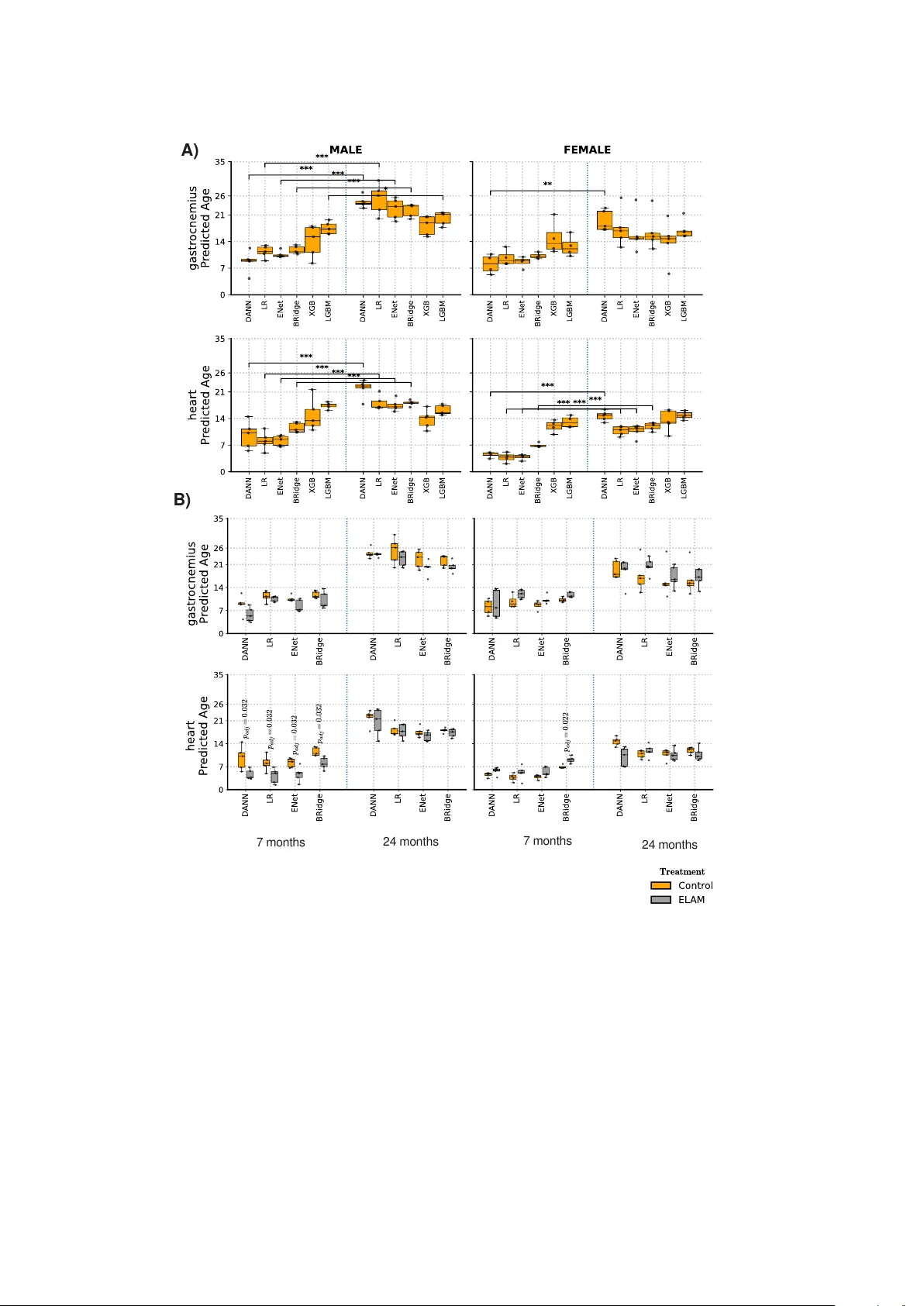
Age Predictors Through the Lens of Generalization, Bias Mitigation, and In terpretabilit y: Reﬂections on Causal Implications Deb das P aul 1* , Elisa F errari , Irene Gravili 1,2 , Alessandro Cellerino 1,2 1 Leibniz Institute on Aging — F ritz Lipmann Institute (FLI), Beuten b ergstr. 11, Jena, 100190, Germany . 2 BIO@SNS, Scuola Normale Sup eriore, Piazza dei Ca v alieri,7, Pisa, 10587, Italy . *Corresp onding author(s). E-mail(s): deb das.paul@leibniz-ﬂi.de ; Con tributing authors: elisa.ferrari.p ersonal@gmail.com ; irene.gra vili@leibniz-ﬂi.de ; alessandro.cellerino@sns.it ; Abstract Chronological age predictors often fail to achiev e out-of-distribution (OOD) gen- eralization due to exogenous attributes such as race, gender, or tissue. Learning an inv ariant represen tation with resp ect to those attributes is therefore essential to improv e OOD generalization and preven t ov erly optimistic results. In predic- tiv e settings, these attributes motiv ate bias mitigation; in causal analyses, they app ear as confounders; and when protected, their suppression leads to fairness. W e coherently explore these concepts with theoretical rigor and discuss the scope of an in terpretable neural netw ork mo del based on adversarial representation learning. Using publicly av ailable mouse transcriptomic datasets, we illustrate the b ehavior of this mo del relative to conv entional machine learning mo dels. W e observ e that the outcome of this mo del is consistent with the predictive results of a published study demonstrating the eﬀects of Elamipretide on mouse sk eletal and cardiac muscle. W e conclude by discussing the limitations of deriving causal in terpretation from such purely predictiv e mo dels. Keyw ords: Representation learning, Adv ersarial training, Out-of-distribution generalization, Bias mitigation, In terpretable machine learning, T ranscriptomics, Aging Clocks 1 List of mathematical notations F or an y scien tiﬁc dissemination, w e believe that it is essential to clarify nota- tions and terminologies in adv ance. In this w ay we can av oid incorrect conclusions, misin terpretations, imprecision, and provide clarit y for the reader. T able 1 : List of notations used in this w ork Notation Description R Set of real num b ers R ≥ 0 Set of nonnegative real num b ers Z Set of integers ⌈ x ⌉ smallest integer greater than or equal to x (Ω , F , P ) Underlying probability space X Input (feature) space Y Output (lab el) space N ( µ , Σ ) Multiv ariate normal distribution on R d X Input random v ariable, X : Ω → X Y Output random v ariable, Y : Ω → Y x, y Realizations of random v ariables X and Y ( X, Y ) Join t random v ariable ( X, Y ) : Ω → X × Y p X,Y Join t probability measure or densit y on X × Y p Y | X Conditional distribution of Y giv en X E [ X ] Exp ectation of X X ⊥ ⊥ Y X and Y are statistically indep endent X  ⊥ ⊥ Y X and Y are statistically dep endent X ⊥ ⊥ Y | Z Conditional indep endence giv en Z E [ Y | X ] Conditional exp ectation E [ Y | X ] = E [ Y ] Mean indep endence of Y from X P Data-generating distribution on X × Y ( x i , y i ) Sample drawn from D { ( x i , y i ) } n i =1 Dataset of size n ( x i , y i ) i.i.d. ∼ P Indep enden t and identically distributed samples S T raining dataset f Prediction function f : X → Y f θ P arameterized predictor with θ ∈ Θ F Hyp othesis class, F ⊆ Y X Θ P arameter space ℓ Loss function ℓ : Y × Y → R ≥ 0 R ( f ) Population risk ˆ R ( f ) Empirical risk on S f ∗ Ba yes-optimal predictor ˆ f Empirical risk minimizer con tinued on next page 2 T able 1 – contin ued from previous page Notation Description do( X = x ) In terven tion setting X to x [ 1 ] p Y | ( X = do ( x )) In terven tional distribution [ 1 ] S Set of sample attributes distinct from input features s ∈ S A ttribute s b elongs to S S bio ⊆ S Set of Biological attributes (e.g., tissue, strain, sex) S exp ⊆ S Set of Exp erimen tal attributes (e.g., platform, proto col, cohort) S prot ⊆ S Set of Protected attributes (e.g., sex, race, ethnicity) List of Deﬁnitions A ttribute: An attribute refers to contextual information asso ciated with a sample that is distinct from the primary feature vector used for prediction. W e denote b y S the set of such attributes and by s ∈ S an individual attribute. These attributes ma y represent biological factors (e.g., tissue or strain), exp erimental conditions (e.g., sequencing platform or proto col), or protected v ariables relev an t for fairness analysis. Sensitive attribute: A sensitive attribute , also referred to as a protected v ari- able , is an attribute whose use in predictive mo dels may lead to discriminatory outcomes for particular groups. Sensitive attributes form a subset S prot ⊆ S . Exam- ples include race, gender, ethnicity , and religion. In fairness-a ware learning, mo dels are often designed so that the learned representation is in v ariant to these attributes. Dataset bias: Dataset bias refers to systematic dep endencies b et ween the learned represen tation and attributes in S that arise from heterogeneous biological or exper- imen tal environmen ts (e.g., tissue type or sequencing platform). Suc h dep endencies ma y degrade out-of-distribution generalization. Metho ds that attempt to remov e or reduce these dep endencies are commonly referred to as bias mitigation tec hniques. Confounder: A confounder is a v ariable Z that c ausal ly inﬂuences both the indepen- den t v ariable X and the dep endent v ariable Y . In such cases the observ ed statistical relationship betw een X and Y do es not reﬂect the true causal eﬀect. F ormally , in a probabilistic setting p Y | X = x  = p Y | do ( X = x ) . Under an appropriate causal model, some attributes in S ma y act as confounders when they causally aﬀect b oth the observed features and the prediction target. Bias mitigation: Bias mitigation refers to learning strategies that reduce undesir- able statistical dep endence b etw een the learned representation and attributes in S . The goal is to encourage represen tations that capture stable predictive signals rather than dataset-sp eciﬁc correlations, thereb y improving robustness and out-of-distribution generalization. 3 Note. Thr oughout the manuscript, we r efer to machine-le arning mo dels that use c hronological age as the target v ariable as age pr e dictors or chr onolo gic al age pr e dictors . This terminolo gy is adopte d to avoid ambiguity and to maintain clar- ity in b oth mathematic al and machine-le arning c ontexts. We do not pr efer to use the term ”clo ck” b e c ause we b elieve this should b e analo gous to fe atur es which describ e the aging pr o c ess - the time evolution. But in the c ommunity term “clo ck” is use d analo- gous to a machine le arning mo del, which is ambiguous. By the wor d attributes , we me an elements in S , unless sp e ciﬁe d explicitly. Con ten ts 1 In tro duction 4 2 Learning in a heterogeneous environmen t E 6 2.1 F rom inv ariance to causalit y . . . . . . . . . . . . . . . . . . . . . . . . 7 2.2 Reic henbac h’s Common Cause Principle (RCCP) - a twist in the tale . 9 3 Confounding and confounders - correlation is not causation 9 4 Generalization under Confounding - unknown vs known 10 5 Confounding, Bias Mitigation, and F airness in Chronological Age Prediction - A Closer Examination 13 6 Domain-Adv ersarial Learning in Deep Neural Netw orks: Mo deling Complex Nonlinear Relationships 15 7 D ANN based Chronological Age Predictor 16 8 Results 17 9 Discussion 22 10 Conclusions 27 11 Materials and Metho ds 27 12 Figure Captions 31 1 In tro duction The problem of chronological age prediction is learning a function f : X → Y , where X is the input feature space, where features can b e genes, proteins, CpGs etc. and Y is the chr onolo gic al age . This is an example of sup ervise d le arning , where the learner is presented with the target lab els, which is the set Y . The c hoice of f is gov erned b y t wo induction principles (rules or assumptions that justify generalizing from ﬁnite observ ations to unseen cases): Empiric al Risk Minimization (ERM) and Structur al 4 R isk Minimization (SRM) [ 2 ]. The term Risk comes from statistical decision the- ory which measures the cost incurred by the learner in doing prediction. The former one seeks the best ﬁtting function to the tr aining data , while the latter one controls the problem of ov erﬁtting. The abov e form ulation of the age prediction problem has mark ed a notable success in the form of famous epigenetic clo ck pioneered b y Stev e Horv ath [ 3 ]. Horv ath identiﬁed a striking asso ciation b etw een DNA methylation pat- terns and c hronological age. Ho wev er, it is now well understoo d within the researc h comm unity that Horv ath’s clo ck do es not provide causal information; rather, it is based on statistical correlation. This conclusion is not derived purely from theoretical considerations but is supp orted by biological kno wledge of the underlying pro cesses go verning DNA meth ylation changes during aging. In what follows, w e examine why a causal interpretation cannot b e established from this asso ciation in theory , and under what assumptions such an interpretation might b ecome plausible. F urthermore, Hor- v ath’s age predictor has already sho wn a remark able predictiv e p erformance across diﬀeren t external test cohorts. How ever, there are instances where the p erformance is sub optimal, for example on ethnicities other than the training p opulations (distinct data-generating processes and en vironments) [ 4 ]. Despite these n uances, Horv ath’s age predictor is still considered to b e a b enchmark. Horv ath’s predictor can b e viewed as a represen tative example of a broader class of linear mo dels trained to predict c hronological age, irresp ectiv e of the speciﬁc biological mo dality from which the fea- tures are deriv ed. F rom a machine learning p ersp ective, such predictors pro vide a tractable and interpretable setting for analyzing the capabilities and limitations of mo dels that rely on chronological age as the sup ervisory signal. W e therefore use this class of predictors as a conceptual lens to inv estigate the limits of age prediction and the conditions under which suc h mo dels succeed or fail. Building on the preceding conceptual analysis, w e revisit an adv ersarial represen tation learning framework based on deep neural netw orks [ 5 ], providing theoretical grounding for why such formula- tions arise naturally when learning representations inv ariant to sample attributes in heterogeneous biological settings. The framework emplo ys an l 1 -based ﬁltering la y er that enables interpretable feature attribution. The adversarial ob jective suppresses attribute-sp eciﬁc information while predicting c hronological age, encouraging repre- sen tations that are less dependent on contextual attributes. By reducing reliance on spurious correlations induced b y suc h attributes, the resulting represen tations improv e out-of-distribution (OOD) generalization across datasets and exp erimental conditions (see Figure 3 ). W e use publicly av ailable mouse transcriptomic datasets (see Materials and Metho ds in Section 11 ) to examine the b ehavior of the adv ersarial framework and to analyze its scop e and limitations relative to conv entional machine learning mo dels. The clinical relev ance of any age predictor mo del is determined by its ability to detect the eﬀect of an interv ention (lifestyle or pharmacological) that leav es a molecular sig- nature (epigenetic, transcriptomic, proteomic, etc.), using the same type of data on whic h the mo del is trained. T o in vestigate this, we selected a published study [ 6 ] in whic h the authors demonstrate the eﬀects of Elamipretide on mouse skeletal and car- diac muscle. When we applied the trained mo del based on the adversarial framework discussed ab ov e to this dataset, w e observed tw o things. First, the mo del was able to diﬀeren tiate b et ween the baseline groups (control vs. treatment) in all cases, whereas 5 the conv entional mo dels failed in at least one case (see Figure 4 A). Second, the mo del indicated rejuvenation, which was rep orted in the study using their in-house age pre- dictor model and is also consistent with other conv en tional mo dels (see Figure 4 B). This observ ation suggests the potential v alue of an ensem ble approach in the future. W e conclude by discussing the p ossible scop e of causal implications (if any) of suc h predictiv e models. W e also reignite the discussion on the need for approac hes with fully data-driv en causal implications in the future, and adversarial represen tation learning ma y represent a step in that direction. In the subsequent sections, w e walk through relev ant theories to rev eal the connec- tions b etw een the concepts of generalization, inv ariance, bias mitigation, fairness, and in terpretability , and how this discussion leads to the adversarial framework presented in this manuscript. These theories are related, but to the b est of our knowledge they ha ve not b een discussed together in a coheren t and systematic manner, particularly in the context of age predictors. 2 Learning in a heterogeneous en vironmen t E Let us consider a prediction problem f : X → Y under multiple environmen ts e ∈ E , i.e., f : X e → Y e . Let F ⊃ E denote a (p ossibly larger) set of en vironments, and the goal is to generalize to previously unobserv ed e ∈ F \ E . In age prediction, suc h en vironments ma y correspond to heterogeneous exp erimental settings, distinct cohorts, tissues, or p opulation-sp eciﬁc data-generating pro cesses, each of whic h can induce distribution shift in the observed features. According to [ 7 ], a common starting point in the in v ariance literature is to assume: (A1) The en vironmen t e do es not directly aﬀect the response, i.e., there is no causal arro w e → Y . (A2) The conditional mec hanism relating cov ariates to the resp onse is stable across en vi- ronmen ts. In practice, this is often more plausible for a subset of features or a learned represen tation Z = Φ( X ) than for the full co v ariate vector, i.e., p Y e | Z e is in v ariant across e . Under such stability assumptions, a linear predictor can b e motiv ated via a w orst- case (robust) L 2 risk ob jective [ 7 ]: ˆ β = arg min β max e ∈F E h ( Y e − X e β ) 2 i , (1) where the expectation is taken under the joint distribution of ( X e , Y e ) in en vironment e . Equation ( 1 ) formalizes pr e dictive r obustness under distributional heterogeneity . Imp ortan tly , links to causal structure arise only under additional assumptions: in v ari- ance can, in certain settings, identify predictors that align with causal parents of Y , but robustness to unseen en vironments should not b e conﬂated with in terven tional causalit y . F rom this viewp oint, the cross-tissue training strategy underlying Horv ath’s epigenetic clo ck can b e seen as encouraging the use of features whose predictive rela- tionship with age is relativ ely stable across tissues; this is consisten t with (but does not by itself prov e) an inv ariance-based explanation for its empirical robustness. More 6 broadly , causal understanding remains essential in aging research b ecause it concerns ho w biological systems respond to p erturbations and interv entions that ma y alter aging tra jectories, whic h go es b eyond predictive stability alone. 2.1 F rom in v ariance to causalit y The follo wing are the tw o inv ariance assumption [ 7 ], whic h provides a sense of causalit y to Equation 1 under linear mo del assumptions: • ( E ): ∃ a subset S ∗ of the cov ariate indices (including the empty set) such that p Y e | X e S ∗ is same ∀ e ∈ E • ( F ): There exists a subset S ∗ and a regression co eﬃcient vector β ∗ with supp ort supp( β ∗ ) = { j | β ∗ j  = 0 } = S ∗ , suc h that, for all e ∈ E , Y e = X e β ∗ + ε e , (2) where the error term ε e is indep endent of X e and ε e ∼ F ε , with F ε denoting the same distribution for all environmen ts e . No w supp ose w e p osit a structur al e quation mo del (SEM) describing the relationship b et ween the random v ariables X and Y that satisﬁes assumptions (A1)–(A2). Under these assumptions, and provided suitable identiﬁabilit y conditions hold, the direct causal paren ts of Y satisfy the corresp onding in v ariance prop erty; see Prop osition 1 in [ 7 ]. In particular, if there exists a subset S ∗ suc h that the conditional distribution p Y e | X e S ∗ remains inv ariant across environmen ts, then S ∗ can b e interpreted as the set of causal paren ts of Y within the assumed SEM. How ever, applying this interpretation to chronological age prediction requires caution. The in v ariance-based causal interpre- tation presupp oses a meaningful SEM in which the co v ariates are direct causes of the resp onse v ariable. In the case of Horv ath’s age predictor, suc h a structural mo del is biologically implausible: chronological age represents elapsed time rather than an out- come generated by molecular mechanisms. The biologically plausible causal direction runs from age to methylation c hanges, not the rev erse. Consequen tly , ev en if an in v ari- an t relationship betw een meth ylation features and chronological age is observed across tissues or environmen ts, this inv ariance should b e interpreted as reﬂecting stable sta- tistical regularities induced by age-driv en molecular processes, rather than evidence that methylation features are causal paren ts of chronological age. 7 Ma r g i n a l c or r e l a ti on R e g r e s s i on I n v a r i a n c e C a u s a l Fig. 1 : Diﬀeren t asso ciations b et ween X and Y as adopted from Figure 12 of [ 7 ] . A marginal correlation is the weak est form asso ciation that ignores dep endencies among cov ariates. A stronger form is the regression relev an t coeﬃcients which captures partial correlation (non-zero correlation co eﬃcients). Causal v ariables are a subset of regression v ariables under faithfulness assumption (A must non-zero co eﬃcien t of all paren ts (direct cause) of Y . In v ariance set is iden tiﬁable ev en when parents of Y not forming a diluted notion of causality . This set is m uch more useful in practical applications as stated in [ 7 ]. Causal form of asso ciation is desirable but often hard to ac hieve. T ak eaw ay : Inv ariance across heterogeneous environmen ts can provide a prin- cipled route to predictive robustness, particularly under shifts in the marginal distribution of cov ariates that lea ve the underlying conditional mechanism stable. Ho wev er, when c hronological age is used as the target v ariable, such stabilit y should not b e conﬂated with causality . Chronological age is an index of elapsed time rather than an outcome generated by molecular features, and the biologically plausible causal direction typically runs from age to molecular c hanges rather than the reverse. Consequently , even predictors that generalize robustly across div erse environmen ts should b e interpreted as capturing in v ari- an t statistical regularities in age-asso ciated biology . Predictive stability under distributional shift do es not, b y itself, establish causal eﬀects, which would require additional structural assumptions or explicit interv entional evidence. In fact, without an y causal assumption (or interv entional v alidation), we can not exp ect any such age predictor will pro vide a causal answer to questions like ”what if and why”. There is currently limited evidence that CpGs used in epigenetic clo cks represen t direct causal drivers of aging [ 8 ]. A goo d wa y to summarize this discussion is Figure 1 , whic h pro vides a pictorial description of diﬀeren t asso ciations b et ween X and Y . 8 2.2 Reic hen bach’s Common Cause Principle (R CCP) - a t wist in the tale Learning based on correlation implies X  ⊥ ⊥ Y . Reichen bach’ s Common Cause Principle states that suc h a dep endence must arise from an underlying causal structure: either X causes Y , Y causes X , or there exists a common cause Z inﬂuencing both [ 9 ]. In the con text of age prediction, the direction X → Y (molecular proﬁle causing c hronological age) lacks biological plausibility . A more realistic explanation is that c hronological age, representing elapsed time, inﬂuences molecular states, i.e., Y − → X , through accum ulated biological pro cesses. Alternatively , latent biological factors suc h as cellular turnov er, metab olic regulation, or damage accumulation may act as common causes Z that jointly inﬂuence both age-asso ciated molecular patterns and phenotypic aging outcomes. Thus, the correlation exploited by age predictors is more plausibly explained by age-driven or shared biological pro cesses rather than molecular fea- tures b eing causal determinants of age itself. This p ersp ective aligns with our earlier in v ariance discussion: in v ariance iden tiﬁes features that stably track age across en vi- ronmen ts, but such stability reﬂects consistent consequences of aging rather than its causes. RCCP bec omes interesting when it connects statistical dep endence to causal- it y through the p ossibility of Z . In mo dern causal terminology , such a common cause corresp onds to a c onfounder . 3 Confounding and confounders - correlation is not causation Confounding is fundamentally a causal concept in which a v ariable, called cofounder, causally inﬂuences b oth the predictor and the outcome, thereb y inducing a non-causal asso ciation [ 10 ] b et ween them. While the term is sometimes used in a purely sta- tistical sense, in this work we adopt the structural (causal) deﬁnition unless stated otherwise. An imprecise use of the term risks in troducing conceptual am biguity and undermining the interpretabilit y of the mo del. F or more deﬁnitions interested readers are referred to [ 11 ]. Presence of confounders (observed/unobserv ed) is a shortcoming in observ ational studies [ 12 ] suc h as ours. But wh y is this imp ortant in our con text? At the beginning, w e discussed tw o induction principles namely ERM and SRM follow- ing which function learning takes place. One of the main reasons that the predictive mo del is sensitive to suc h spurious correlation is due to ERM. ERM fails to distin- guish causal vs non-causal signals b ecause it minimizes a verage risk. ERM ma y uses a non-causal shortcut path to pro vide better accuracy for the test set sharing same distribution as that of the training [ 10 ], but fails for an external dataset where this shortcut is missing. Suc h failures often arise under distribution shifts, particularly when the condi- tional mechanism changes (concept shift, p e Y | X  = p e ′ Y | X ). While confounding is one p ossible source of spurious asso ciations, other mec hanisms suc h as selection bias or rev erse causation may also induce non-causal dep endencies. The discrepancy b et ween 9 high in-distribution p erformance and p o or robustness under distribution shift there- fore motiv ates learning principles that go b eyond ERM and explicitly seek stable relationships across en vironmen ts, as emphasized in in v ariance-based approac hes. This discrepancy b etw een in-distribution accuracy and robustness under distribution shift motiv ates a closer examination of generalization in the presence of spurious asso ciations, including confounding. 4 Generalization under Confounding - unkno wn vs kno wn The task of making accurate predictions on test data drawn from either the same distribution as the training data (in-distribution) or from a diﬀerent distribution (out- of-distribution) is referred to as in-distribution (ID) and out-of-distribution (OOD) generalization, resp ectively . Age predictors often fail to adequately address the OOD c hallenge [ 4 , 13 – 17 ], whic h limits the robustness of their predictions and reduces the clinical relev ance of the learned feature representations. But success of a predictive mo del lies in its p ow er to predict in a new context. Unfortunately , the problem of OOD generalization is an il l-p ose d problem. A problem is ill-p osed when either of the follo wing is applicable: • Unique solution do es not exist • Unique solution exists but computationally not feasible • Unique solution exists but unreliable. In the presence of unkno wn confounders, OOD generalization b ecomes fundamen- tally infeasible. In particular, the ERM principle tends to exploit spurious correlations presen t in the training data, which may not persist under distribution shifts. As a result, ev en when a unique solution exists, it ma y fail to generalize reliably b eyond the training distribution. Therefore, we require principled approaches that enable mo dels to generalize reliably under out-of-distribution settings. When the set of confounders C is observ ed, one can mo del the conditional mec hanism p Y | X,C instead of p Y | X . Under the assumption that C satisﬁes the bac kdo or criterion relative to ( X , Y ), conditioning on C blocks spurious dep endence induced b y common causes, i.e., Y ⊥ ⊥ X | do( X ) , C and p Y | do( X ) ,C = p Y | X,C . Th us, adjusting for C remov es bias due to confounding and allows the conditional mec hanism to b etter reﬂect the underlying causal or stable predictive relationship. In this case, the learning problem b ecomes b etter p osed, as part of the ambiguit y in the X – Y relationship can b e resolved through adjustment. How ever, OOD generalization remains c hallenging: shifts in the distribution of C , changes in the conditional mech- anism p Y | X,C , or measuremen t noise in C ma y still impair robustness. A v ariety of strategies hav e been prop osed to improv e out-of-distribution (OOD) generalization, 10 including domain adaptation (DA) [ 18 ], domain generalization (DG) [ 19 , 20 ], and distributional robust learning (DRO) [ 21 – 23 ]. T ak eaw ay : F or an age predictor to generalize reliably in OOD settings with hidden confounding , identifying an inv ariant set of features is necessary but not suﬃcien t. Robust generalization additionally requires accoun ting for en vironment-speciﬁc v ariation and p otential shifts in the data-generating pro- cess - a problem that can b e addressed using framew orks suc h as the domain adaptation (DA) . W e will now discuss DA—it’s underlying assumptions and inheren t limitations. Most imp ortantly , D A pro vides the conceptual foundation for our prop osed age predictor, which we introduce in the subsequent sections. Domain adaptation (DA) D A considers tw o domains: a source domain and a target domain, asso ciated with probabilit y distributions P s and P t o ver the input–lab el space X × Y , with P s  = P t . The learner is given lab eled source samples { ( x s i , y s i ) } n s i =1 i.i.d. ∼ P s , and unlab eled target inputs { x t j } n t j =1 i.i.d. ∼ P t X , where P t X denotes the marginal of P t o ver X . The ob jective is to learn a predictor f : X → Y that achiev es low target risk R t ( f ) = E ( X,Y ) ∼P t [ ℓ ( f ( X ) , Y )] , despite ha ving access to lab els only from the source domain. The learned mo del is required to p erform the same pr e diction task on the target domain. In the context of age prediction, this task corresponds to estimating c hronological age from molecular features. The model is expected to exploit source domain knowledge and the similarit y b et ween t w o domains when p erforming the task on the target domain. Since this is an instance of OOD generalization, the goal is to learn a common represen tation of b oth the domains so that w e can exploit the assumption of the discriminative classiﬁer: the training and test data comes from the same distribution. A t this setting w e can use the ERM principle. Rather than formalism, w e are mainly interested in the assumptions of DA which will provide us practical limitations. The authors in [ 24 ] sho w that, without additional relatedness assumptions, successful domain adaptation cannot b e guaranteed. One key quan tity that app ears in domain adaptation theory is a h yp othesis-class–dep endent discrepancy betw een the source and target mar ginal 11 input distributions, commonly deﬁned via the H ∆ H -divergence [ 18 ]: d H ∆ H ( P s X , P t X ) = 2 sup h,h ′ ∈H    E x ∼P s X [ I { h ( x )  = h ′ ( x ) } ] − E x ∼P t X [ I { h ( x )  = h ′ ( x ) } ]    . (3) Here, P s X and P t X denote the marginal distributions ov er the input space X induced b y the source and target domains, resp ectively . The function I { h ( x )  = h ′ ( x ) } is the indicator of disagreement b etw een tw o hypotheses h, h ′ ∈ H on input x . This form ulation assumes binary-v alued h yp otheses h : X → { 0 , 1 } for simplicity . F urthermore, there m ust b e a single h yp othesis (predictor) that works w ell (ha ving minim um error) in both the domains. These tw o assumptions together are suﬃcient for DA to w ork whic h is evident from the following inequalit y according to Theorem 2 in [ 18 ]: ϵ t ( h ) ≤ ϵ s ( h ) + 1 2 d H ∆ H  P s X , P t X  + λ (4) where λ = min h ′ ∈H  ϵ s ( h ′ ) + ϵ t ( h ′ )  denotes the join t error of the optimal shared h yp othesis in H . In Equation 4 , the cen tral quantit y gov erning out-of-distribution per- formance is the H ∆ H divergence. F or a ﬁxed hypothesis class H , this term measures the maxim um discrepancy in disagreement rates betw een pairs of hypotheses h, h ′ ∈ H across the source and target domains. Consequently , the divergence is small when h yp otheses exhibit similar disagreement patterns on both domains. If a representation can b e learned in whic h samples from the source and target domains b ecome indistin- guishable, then even the worst-case domain discriminator fails, leading to a reduction of the H ∆ H divergence. Imp ortantly , since target lab els are unav ailable during train- ing, the learner cannot directly optimize target-domain error. Instead, representation learning induces a trade-oﬀ b et ween minimizing the source-domain error and reducing the divergence term using unlab eled target data. T ak eaw ay : The generalization b ound for DA reveals fundamental limitations of age predictors under distributional shift. T arget-domain error is go verned not only by in-distribution performance, but also b y the discrepancy b etw een training and deploymen t en vironments, as measured b y the H ∆ H divergence, and by the existence of a hypothesis that generalizes across domains. In age prediction, shifts in the data-generating en vironmen t—such as c hanges across tissues, cohorts, sequencing proto cols, or demographic groups—can induce large divergences, even when empirical risk on the training data is low. The preceding discussion naturally leads to an adv ersarial learning frame- w ork . Speciﬁcally , a feature transformation is learned to pro ject the original inputs in to a laten t space in which samples from the source and target domains are indis- tinguishable, thereb y minimizing the divergence term in Equation 4 . Simultaneously , a domain discriminator is trained to maximize domain separability from the same laten t represen tation. This resulting min max optimization deﬁnes the adversarial D A framew ork. By construction, this adversarial ob jectiv e suppresses features that are 12 informativ e of domain iden tity , whic h are precisely the features that often give rise to spurious correlations. As such correlations enco de information ab out wher e a sample originates rather than what is being predicted, their remo v al encourages reliance on domain-in v ariant and more stable predictive signals. T ak eaw ay : Adversarial D A is directly motiv ated b y Equation 4 , as it seeks to reduce domain-informativ e, spurious v ariation b y learning represen tations in whic h source and target samples are indistinguishable. While such adversarial in v ariance can mitigate confounding and improv e robustness, genuine biological heterogeneit y may still induce a large irreducible error term λ , fundamentally limiting reliable out-of-distribution generalization. 5 Confounding, Bias Mitigation, and F airness in Chronological Age Prediction - A Closer Examination The preceding discussion framed domain-adversarial learning as a mechanism for suppressing domain-speciﬁc v ariation and promoting represen tations that capture pre- dictiv e structure inv ariant across en vironments. In man y practical learning settings, ho wev er, domain identit y is often correlated with biological or demographic attributes (e.g., cohort, tissue, ancestry , or health status). Consequently , suppressing domain- informativ e signals do es not only address robustness to distribution shift; it ma y also inﬂuence how learned representations dep end on group-level attributes. This obser- v ation highlights an important conceptual distinction, particularly in the context of c hronological age prediction. Attributes asso ciated with domain heterogeneity S exp and S bio ma y introduce dataset bias (see List of Deﬁnitions), correspond to S prot relev ant for fairness considerations, or—under an appropriate causal model—act as confounders inﬂuencing b oth the observed features and the prediction target. Although these p ersp ectives arise from diﬀerent motiv ations, they share a common concern: con trolling ho w learned represen tations dep end on auxiliary attributes. While these ob jectives may o verlap, they arise from diﬀerent motiv ations and require separate examination. W e therefore brieﬂy discuss fairness and its relation to in v ariance and domain adaptation. The concept of fairness plays a crucial role in artiﬁcial intel- ligence (AI), particularly in the subﬁeld of mac hine learning, where systems are increasingly used for decision-making. In this con text, fairness generally means that a decision-making process should not rely on the set S prot (see List of Deﬁnitions and Mathematical Notations). In other words, decisions pro duced by AI systems should b e indep enden t of the set S prot and should not disadv an tage individuals or groups based on them. There are three widely studied notions of fairness in machine learning: individual fairness, group fairness, and coun terfactual fairness[ 25 ]. • Individual fairness requires that similar individuals b e treated similarly . That is, if tw o individuals are alike with resp ect to all task-relev ant attributes, then the mo del’s predictions for them should b e identical or diﬀer only negligibly . F or 13 example, t wo individuals of the same age but diﬀeren t genders should receive nearly the same predicted age. • Group fairness fo cuses on statistical parity across predeﬁned groups. Under this notion, diﬀerent demographic groups—suc h as groups deﬁned b y ethnicit y or gen- der—should, on a verage, receive similar outcomes. F or instance, individuals of the same age b elonging to diﬀerent ethnic groups should hav e comparable predicted ages when aggregated at the group level. • coun terfactual fairness is based on causal reasoning and requires that a mo del’s prediction for an individual remain unchanged in a counterfactual world in which the individual’s s ∈ S prot are altered while all other relev ant factors are held constant. In other words, any element of S prot should not causally inﬂuence the decision outcome. F airness is particularly relev ant in age prediction tasks b ecause the input features X may b e correlated S prot . Although these attributes do not causally determine c hronological age, biological and environmen tal diﬀerences across groups can inﬂu- ence molecular measuremen ts used for prediction. F airness considerations therefore do not require identical predictions across groups, but rather that the predictor do es not exhibit systematic bias or unequal error patterns with respect to S prot . A fairness- a ware age predictor seeks representations that maintain predictiv e v alidity while a voiding consisten t ov er- or under-estimation for sp eciﬁc demographic or biological subp opulations. In our opinion, chronological age prediction from molecular proﬁles should explic- itly consider the sample-attribute set S (e.g., tissue, strain, platform, proto col, sex, gender, ethnicity etc.), s ince v ariation in these attributes can induce spurious, en vironment-speciﬁc asso ciations and degrade out-of-distribution generalization. The term c onfounder mitigation should therefore b e used cautiously in this predictive set- ting unless an explicit causal estimand is deﬁned. In practice, controlling dep endence on elements of S is more appropriately framed as bias mitigation when the attributes b elong to S exp and/or S bio (e.g., tissue or platform), and as fairness-awar e le arning when the attributes b elong to S prot . F or example, [ 26 ] describ es gender as a confounder while predicting c hronological age; under the classical causal deﬁnition this is not strict confounding, and Figure 5a uses double-headed arrows indicating statistical dep en- dence rather than causal inﬂuence. A more precise interpretation is that gender can induce group-dep enden t statistical structure in the data, motiv ating inv ariance-based represen tation learning to reduce reliance on unstable or group-sp eciﬁc correlations rather than to correct confounding in the causal sense. So where does the confusion lie? The conceptual confusion in so called clo c k researc h arises b ecause chronological age pla ys tw o distinct roles. During mo del train- ing, age functions as an observ able time index, leading to a predictive task in which age causally precedes many molecular changes. In this setting, the learned mapping from molecular features X to age Y is fundamentally a statistical asso ciation, and classical confounding with respect to chronological age is unlik ely . Ho wev er, this predictiv e rela- tionship is often reinterpreted biologically: clock outputs are treated as pro xies for a laten t biological aging state, a causal quan tit y that ma y itself be inﬂuenced b y genetic, en vironmental, and demographic factors. This shift in interpretation implicitly changes 14 the causal target—from an observ able time v ariable to an unobserved biological pro- cess—while the model w as trained only on c hronological age. Because the predictiv e direction X → Y is opp osite to the plausible causal direction Y → X , it b ecomes easy to mistake strong statistical asso ciations for mechanistic relationships. As a result, terminology from causal inference, such as confounding, is sometimes applied to what is essentially a predictiv e asso ciation problem, even though the underlying causal structure diﬀers b et ween the training ob jective and the biological interpretation. 6 Domain-Adv ersarial Learning in Deep Neural Net w orks: Mo deling Complex Nonlinear Relationships Age-related molecular data, such as gene expression or methylation proﬁles, are high- dimensional and exhibit complex nonlinear structure. Simple linear mo dels may fail to capture these patterns, motiv ating the use of deep neural net works for age pre- diction. How ev er, deep mo dels are particularly prone to exploiting dataset-speciﬁc signals—suc h as platform eﬀects, batc h artifacts, or cohort-sp eciﬁc biases—when trained under empirical risk minimization. As discussed earlier, such reliance on domain-sp eciﬁc structure leads to p oor generalization under distribution shift and corresp onds to a large H ∆ H -distance b etw een domains. T o address this c hallenge, domain adaptation metho ds ha ve been extended to deep learning frameworks through representation learning. The key idea is to learn fea- ture representations that remain predictiv e for the primary task (here, age prediction) while suppressing information ab out domain iden tity . In 2015, Y aroslav Ganin and Victor Lempitsky [ 27 ] prop osed Domain-Adv ersarial Neural Net works (DANN), a metho d that in tegrates adversarial training into neural netw orks to encourage domain-in v ariant representations. This approach enables domain adaptation in high- dimensional settings such as transcriptomics, where nonlinear structure and complex feature interactions are prev alent. Using a tec hnique called gr adient r eversal , they sho wed that adversarial training of a domain classiﬁer encourages the feature extrac- tor to reduce the H ∆ H -distance b etw een source and target domains (cf. Equation 13 in [ 27 ]). In tuitively , this makes samples from diﬀerent datasets harder to distinguish in the learned represen tation. In this sense, hiding domain information via the feature extractor is analogous to learning a fair r epr esentation with resp ect to S prot (same for mitigating bias or confounders dep ending on whic h set of attributes are consid- ered): the mo del is encouraged to discard v ariation related to dataset iden tity while retaining information relev ant for the prediction task. Learning complex patterns and non-linear relationships b et ween S and the set of features p o orly handled by clas- sical machine learning approaches equipp ed with batch eﬀect corrections and other prepro cessing tec hniques. Aging falls into this sp eciﬁc case, especially when the data are transcriptomic—high-dimensional and noisy , with complex nonlinear relationships with tissue type, cell comp osition, technical platform, and other biological and exp er- imen tal co v ariates. In such settings, the aging signal is embedded within a mixture of interacting sources of v ariation, making it diﬃcult to isolate using simple linear or additive mo dels and motiv ating the need for representation learning approaches 15 that can capture structured, nonlinear patterns. D ANN has later been exploited to learn an inv ariant representation with resp ect to S [ 28 ] and also shown to b e eﬀectiv e in practical applications of predictive mo deling suc h as in [ 26 ]. The authors further p oin ted out that learning representation inv ariant to S while obtaining an optimal classiﬁer/regressor is imp ossible when elements in S and the target v ariable are statis- tically dep endent, as also p ointed out in [ 29 ]. In fact, the learned representation ma y still leak information regarding s ∈ S even after strengthening adversarial training [ 30 ]. 7 D ANN based Chronological Age Predictor Building on the strategies discussed ab ov e, and guided by their theoretical sound- ness as well as practical applicability , we adopt these approaches in the form of a D ANN based mo del to address age prediction while explicitly promoting bias miti- gation, generalization, fairness and in terpretabilit y . Of note, the model emplo yed for transcriptomic age prediction was originally prop osed in [ 5 ] by the second and the last authors of this current manuscript. In this work, we are examining it within a more explicit theoretical con text, clarifying its prop erties and discussing its scop e and limitations for bias mitigation, fairness, OOD generalization, and interpretabilit y . W e further illustrate its practical applicabilit y through an interv entional case study (see Section 8 ) inv olving skeletal and cardiac m uscle tissues, which mo del tw o distinct age- asso ciated pathoph ysiological contexts: sarcopenia and cardiometab olic dysfunction, resp ectiv ely . The input is the gene expression data and the output is the chronological age. The goal is to learn a debiase d and/or fair representation with resp ect to S . One imp ortan t addition to our deep neural net based arc hitecture is a Binary Sto chastic Filter (BSF) [ 31 ] lay er at the b eginning of the enco der (see Metho ds). The BSF mim- ics the l 1 regularization during the training phase of the neural net w ork, helps to learn predictiv e genes - ensuring in terpretability . It is w orth noting that most curren t age predictors based on transcriptomic data only partially address the issue of mitigating the eﬀect of S in prediction. F or instance, the BiT Age clock in C. ele gans [ 32 ] uses binarization to reduce noise, but do es not include explicit fairness strategies. Deep learning–based mo dels developed for human bulk transcriptomes [ 33 ] primarily emphasize predictive accuracy , without incorp o- rating debiasing mechanisms. Some single-cell approaches [ 34 ] apply batch correction during preprocessing, but rely on p ost hoc adjustments rather than in tegrating bias mitigation into mo del training. Similarly , clocks trained on brain-sp eciﬁc [ 35 ] or tissue- sp eciﬁc [ 36 ] datasets limit heterogeneity by restricting the scop e of the data, but do not directly address confounding during learning. In con trast, D ANN explicitly includes elemen ts of S in the training pro cess. It requires minimal prepro cessing (see Materials and Metho ds), does not assume a particular prior distribution of the data, and sup- p orts the iden tiﬁcation of biologically relev ant features in a m ulti-tissue setting. While adv ersarial learning and sto chastic ﬁltering are well-established individually , combin- ing them in to a uniﬁed framework is nontrivial. W e therefore view this integration as a metho dological contribution. Importantly , w e present our results in a balanced manner, highlighting not only the strengths of the approach but also its limitations in ligh t of the theoretical considerations discussed ab ov e. W e b elieve that ackno wledging 16 b oth asp ects is essen tial for the comm unity to understand the constrain ts of current age predictors and to make careful claims ab out their scop e and applicability . 8 Results Adv ersarial Learning of S -Inv arian t Represen tation In the adversarial representation learning framework describ ed in Section 11 , the enco der ( FE ) and the bias predictor ( BP ) in Figure 2 A engage in a zero-sum game. The bias predictor ( BP ) aims to infer s ∈ S from the laten t represen tation F , while the enco der ( FE ) attempts to conceal this information resulting into a minimax optimiza- tion problem whic h seeks a saddle p oint where the representation remains predictiv e of age but in v arian t to S . Ideally , the categorical cross-en tropy loss of BP should decrease during training. How ever, when adv ersarial training is activ e (i.e., α > 0), the loss increases and even tually stabilizes (Figure 2 B, second row), indicating that the enco der successfully suppresses attribute related information in the laten t space. In contrast, when adversarial training is disabled ( α = 0), the loss decreases sharply , demonstrat- ing that the protected or nuisance attributes can b e readily predicted from the latent represen tation. This b eha vior is further reﬂected in Figure 2 C, which shows the corre- lation b etw een predicted and true v alues of the attributes (one-hot enco ded). The loss dynamics and correlation patterns across training epo c hs collectively indicate that the adv ersarial approach eﬀectiv ely mitigates bias asso ciated with these attributes. W e further ev aluate predictive p erformance on holdout datasets (Figure 2 D) and assess the co eﬃcien t of v ariation (CV) across datasets for diﬀerent v alues of α . W e observe that the CV of the mean absolute error (MAE) is consistently low er for α > 0, indi- cating improv ed stability under distribution shift. This trend is less consisten t for R 2 , except at α = 50 (see Section 9 for further discussion). In terpretable Learning via Binary Sto chastic Filtering Without Signiﬁcant P erformance Loss A Binary Sto c hastic Filter (BSF) [ 31 ] is introduced at the input of the enco der to pro- mote feature sparsiﬁcation. The BSF lay er operates by m ultiplying e ac h input feature b y a binary v ariable z j ∈ { 0 , 1 } , where z j is sampled from a Bernoulli distribution parameterized by a learned con tinuous w eight w j . During training, the probabilit y of retaining feature j is therefore adaptiv ely up dated, allowing the mo del to sto chastically explore diﬀeren t feature subsets. After training, a user-deﬁned threshold is applied to w j to obtain a deterministic binary mask, yielding a ﬁxed subset of selected genes for prediction (see Mo del architecture in Section 11 for details). This mechanism eﬀectively reduces the dimensionality of the input space while retaining features that contribute most to predictiv e p erformance. Empirically , incor- p orating the BSF la y er leads to a substan tial reduction in the n umber of genes without degrading performance and, in sev eral cases, yields impro ved results compared to clas- sical machine learning models (Figure 3 B). When compared to the non-ﬁltered deep 17 F Feature extractor Bias predictor Data Classi ﬁ er/Regressor A ) B ) C ) D ) Fig. 2 : F or detailed caption, see Section 12 18 mo del, p erformance remains comparable and o ccasionally improv es (Figure 3 C), sug- gesting that sparsiﬁcation can mitigate ov erﬁtting in high-dimensional settings rather than merely eliminating predictive signal. W e also observe low er co eﬃcients of v ariation (CV) for MAE and R 2 across datasets when the BSF la y er is applied, indicating impro ved stability under dataset heterogene- it y . Ho w ever, CV should b e in terpreted with caution: a low CV does not necessarily imply superior robustness, as it dep ends jointly on the mean and disp ersion of the metric. Therefore, improv emen ts in stability should b e ev aluated alongside absolute predictiv e p erformance rather than considered in isolation. Binary Sto c hastic Filter Selects Genes with Contextual Relev ance F or eac h holdout dataset, we identiﬁed the set of genes selected b y the Binary Stochas- tic Filter in each v alidation fold. W e then determined the intersection (common subset) of selected genes across folds to obtain a stable gene set. This consensus gene set w as subsequen tly submitted to the STRING database ( https://string- db.org ) for functional enrichmen t analysis, and KEGG pathw a y enrichmen t w as computed for the selected genes. Across holdout settings, w e noticed that the attributed genes w ere frequently signiﬁcant and consistent with w ell-established aging mec hanisms (see Figure 4 ). In particular, pr otein pr o c essing in the endoplasmic r eticulum (ER proteostasis/UPR) and autophagy repeatedly emerged, aligning with the recognized roles of proteostasis decline and impaired macroautophagy in aging [ 37 – 39 ]. W e also observ ed recurren t enrichmen t of the p53 signaling p athway , consisten t with extensive evidence linking DNA damage resp onses, cellular senescence, and p53 netw ork activ- it y to aging phenot yp es [ 40 ]. T erms related to RNA handling were also prominen t, including RNA tr ansp ort and, in some holdouts, splic e osome . These results are concor- dan t with rep orts that age-asso ciated changes in RNA metab olism, including altered n uclear mRNA export and splicing dysregulation, con tribute to cellular aging and age- related disease [ 41 – 43 ]. W e also noticed that, mTOR signaling w as enriched, which is consisten t with the central role of n utrient-sensing pathw ays and mTOR in regulating aging and longevity . [ 37 , 44 ]. Finally , enrichmen t of cir c adian rhythm in one case is compatible with growing evidence that circadian disruption and age-dep endent clo c k output reprogramming are linked to aging and systemic decline [ 45 , 46 ]. Overall, the recurrence of these pathw ays across independent holdouts supp orts the biological plau- sibilit y of the attribution-deriv ed gene sets and pro vides a pathw ay-lev el interpretation of mo del b eha vior. D ANN Captures Baseline Diﬀerences Across Conditions more Eﬀectiv ely than Con v en tional Regression and T ree-based Approac hes The ultimate test of an age-prediction mo del, in terms of practical applicability , is its abilit y to detect the eﬀects of pharmacological interv entions at the same level of abstraction as the input data (e.g., transcriptome or epigenome). T o this end, we considered a recent study b y Mitc hell et al. [ 6 ], whic h inv estigated the eﬀects of the 19 Binary Stochastic Filter (straight through estimator) F F eature extr actor Bias predictor Data Classifier/R egressor B ) C ) D ) E ) A ) Fig. 3 : F or detailed caption, see Section 12 20 holdout: GSE145480 holdout: GSE75192 holdout: GSE1111164 0.4 0.6 0.8 1.0 1.2 1.4 Signal Protein processing in endoplasmic reticulum Spliceosome p53 signaling pathway Ubiquitin mediated proteolysis Autophagy - animal RNA transport NF-kappa B signaling pathway RNA degradation Nucleotide excision repair Small cell lung cancer Groups at similarity 0.8 1.0e-02 1.0e-03 1.0e-05 1.0e-07 1.0e-08 1.0e-10 FDR 10 20 30 40 Gene count 0.35 0.40 0.45 0.50 0.55 0.60 0.65 0.70 Signal Protein processing in endoplasmic reticulum p53 signaling pathway Colorectal cancer Ubiquitin mediated proteolysis RNA transport Endometrial cancer Autophagy - animal Spliceosome Platinum drug resistance mT OR signaling pathway Groups at similarity 0.8 2.9e-03 1.0e-03 3.3e-04 1.1e-04 3.8e-05 1.2e-05 FDR 10 20 30 Gene count 0.4 0.5 0.6 0.7 0.8 0.9 1.0 1.1 1.2 Signal Protein processing in endoplasmic reticulum p53 signaling pathway Basal transcription factors RNA transport Spliceosome Ribosome biogenesis in eukaryotes Platinum drug resistance Autophagy - animal Nucleotide excision repair Circadian rhythm Groups at similarity 0.8 1.0e-02 1.0e-03 9.0e-05 7.0e-06 5.0e-07 3.0e-08 FDR 10 15 25 35 Gene count Fig. 4 : F or detailed caption, see Section 12 21 ELAM peptide on sk eletal and cardiac m uscle in male and female mice at 7 and 26 mon ths of age (the age when the samples for sequencing are collected). The authors observ ed that functional improv ements induced by ELAM did not alwa ys translate in to clear transcriptomic or epigenetic shifts, and accordingly , the chronological age predictor based on a Ba yesianRidge transcriptomic clo ck trained on a large external dataset did not strongly reﬂect in terv ention eﬀects [ 47 ]. It is imp ortant to note that the transcriptomic clo c k used in that study w as trained on a substan tially larger corpus than our o wn model; our dataset represents a smaller subset of the training data used in [ 47 ]. Despite this relative data scarcity , our mo del was able to distinguish b et ween con trol groups at baseline (see Figure 5 A) and exhibited p erformance that aligns with other classical predictors (see Figure 5 B). This suggests that representation learning com bined with fairness mitigation can ac hieve robust generalization even with limited training data — a setting that is often prone to ov erﬁtting and spurious correlations [ 48 ]. 9 Discussion The primary ob jective of this manuscript is to examine OOD generalization, bias mitigation, fairness, and interpretabilit y as key prop erties of c hronological age predic- tors—mac hine learning mo dels in whic h c hronological age is used as the target v ariable and is often treated as a proxy for biological age. These models are now widely applied in aging research, yet it is often unclear under what conditions such predictors general- ize across heterogeneous biological settings, whether their errors diﬀer systematically across groups (e.g., sex or exp erimen tal cohorts), and to what extent their learned structure allows meaningful biological interpretation. F urthermore, the assumptions that implicitly connect these properties to causal reasoning are rarely made explicit. By clarifying these issues, w e aim to pro vide a more principled understanding of what c hronological age predictors capture—and what they do not or can not without further assumptions. Scop e of Causal Interpretations of Chronological Age Predictor It is widely ackno wledged that chronological age prediction is not causal in the inter- v entional sense, the precise implications of this statement are rarely articulated. Under the inv ariance framew ork of [ 7 ], causal in terpretation arises when there exists a struc- tural equation mo del in whic h the resp onse v ariable is generated b y its direct causes through an in v arian t mec hanism across en vironments. In such settings, inv ariance can iden tify the causal paren ts of the resp onse. How ever, when chronological age serv es as the target v ariable, the structural premises required for this interpretation are biolog- ically implausible. Chronological age represents elapsed time rather than an outcome generated b y molecular features; the biologically plausible direction of causation runs from age to molecular changes, not the reverse. Consequen tly , even if assumptions (A1)–(A2) in Section 8 hold statistically and predictive relationships remain in v ariant across heterogeneous en vironments, this inv ariance cannot b e interpreted as evidence that molecular features are causal parents of chronological age. Instead, robust age predictors should b e understo o d as capturing stable statistical regularities induced 22 7 months 7 months 24 months 24 months A) B) Fig. 5 : F or detailed caption, see Section 12 23 b y age-driven biological pro cesses. An y stronger causal in terpretation would require additional structural assumptions or explicit in terven tional v alidation. Generalization, Confounding, Domain Adaptation, Adversarial Learning using DNN In order to hav e a coheren t narrative, we started from the p ersp ective of learning under distributional heterogeneity . W e highligh ted the assumptions based on which linear predictors may approximate inv ariant relationships across e n vironments and when they instead capture environmen t-sp eciﬁc or spurious associations. This leads naturally to a discussion of generalization in the presence of latent structure, which w e discussed in Section 4 . In this con text, w e argue that the term c onfounding m ust be used with caution when chronological age is the resp onse v ariable. Since chronological age is not manipulable in the standard causal sense, classical confounding do es not directly apply . Instead, systematic group-dep endent diﬀerences in prediction errors are more appropriately framed within a fairness p ersp ectiv e. W e therefore reinterpret certain phenomena commonly describ ed as “confounding” as issues of fairness miti- gation and pro vide justiﬁcation for this distinction. Among the diﬀeren t strategies to impro ve out-of-distribution (OOD) generalization, we focus on a domain adaptation (D A) framework. This choice is motiv ated b y the fact that our ﬁnal model is based on adversarial represen tation learning, which naturally aligns with DA principles. By encouraging domain-in v ariant representations, the mo del reduces dataset-sp eciﬁc eﬀects in transcriptomic data. One may argue that domain generalization (DG) is more appropriate, since in DG the target domain is unknown during training and no adaptation is p ossible. This is indeed the ideal scenario, as the mo del should general- ize to unseen domains without retraining. Although our approach is inspired by D A, its goal is consisten t with DG: to learn represen tations that generalize across domains. Exploring dedicated DG metho ds in this setting is an imp ortant direction for future w ork. Adv ersarial approac h - without and with Binary Sto chastic Filter vs. Classical Machine Learning Mo dels While adv ersarial regularization eﬀectiv ely reduces the correlation b et ween the latent represen tation and nuisance attributes (Figure 2 C), its impact on cross-dataset sta- bilit y is neither uniform nor strictly monotonic. In particular, α = 0 can still yield relativ ely low co eﬃcien ts of v ariation (CV) in some settings (Figures 2 D, 3 D, SA2 and SA3 ). This is not contradictory . When distributional diﬀerences across holdout datasets are limited—suc h as predominantly cov ariate shifts that do not substantially alter the conditional relationship betw een features and age—standard empirical risk minimization may already generalize adequately . Moreov er, if dataset-sp eciﬁc correla- tions are shared across en vironments, exploiting them may not immediately degrade cross-dataset performance. Thus, the b eneﬁt of adv ersarial regularization becomes more pronounced when heterogeneit y reﬂects mec hanism shifts or group-sp eciﬁc struc- ture rather than mild distributional v ariation. It is also important to interpret CV cautiously . Since CV is computed o ver dataset-level mean metrics, it is sensitive to the 24 n umber of datasets and to diﬀerences in outcome v ariance across cohorts. This is par- ticularly relev ant for R 2 , which depends explicitly on the v ariance of chronological age within eac h dataset and may ﬂuctuate even when the absolute prediction error (MAE) remains stable. The more consistent reduction of CV observed for MAE therefore pro- vides stronger evidence for impro ved robustness than R 2 alone. T aken together, these observ ations suggest that adversarial regularization promotes representation-lev el in v ariance, whic h can translate into improv ed cross-dataset stability when heterogene- it y is driv en by nuisance structure. How ever, the eﬀect depends on the magnitude and nature of distributional diﬀerences, and increasing α does not guarantee monotonic impro vemen t. Excessiv ely strong adv ersarial constrain ts ma y suppress useful predic- tiv e signal alongside n uisance information, underscoring the need for principled tuning rather than assuming uniform beneﬁt for all α > 0. Complementing this, the BSF lay er addresses a related but distinct s ource of instability: high-dimensional redundancy . By inducing sparsity through l 1 -regularization and thresholding (see Section 11 ), the ﬁlter restricts the mo del to a smaller, more informative subset of features. This reduc- tion of representational capacit y can limit ov erﬁtting to dataset-sp eciﬁc patterns and, when appropriately tuned, main tain or ev en improv e predictive p erformance compare to the scenario when the entire set of features are used. Importantly , adversarial inv ari- ance and feature sparsiﬁcation op erate through diﬀerent mechanisms—one suppresses group-dep enden t information in the latent space, while the other constrains feature complexit y—yet both aim to enhance robustness under heterogeneit y . Their com bined eﬀect suggests that stability across datasets is achiev ed not by eliminating signal, but b y selectively retaining inv arian t and informative structure. It should be noted that although no automated h yp erparameter optimization (e.g., Optuna [ 49 ]) was p erformed for the adversarial framew ork, we were able to iden- tify conﬁgurations that impro ved cross-dataset robustness relative to classical mo dels ev aluated under default scikit-learn settings. This observ ation should not b e inter- preted as evidence of universal sup eriority . Rather, it suggests that the adversarial arc hitecture introduces an inductive bias aligned with the structured heterogeneit y presen t in biological aging data. Classical mo dels optimized solely for empirical risk ma y implicitly enco de dataset-sp eciﬁc correlations, whereas the adversarial constraint explicitly discourages suc h dependence. Consequen tly , the observ ed impro vemen ts lik ely reﬂect structural alignment b etw een the imp osed inv ariance constraint and the data-generating characteristics, rather than an inherent adv antage indep enden t of tun- ing eﬀort. A balanced h yp erparameter optimization across mo del classes w ould pro vide a more deﬁnitive comparison. A ttributes are Reco v erable using a P ost-ho c Classiﬁer The primary goal of the adversarial learning mo del, as describ ed in Section 11 under Materials and Metho ds, is to promote fairness in the learned latent represen tation. As sho wn in Figure 2 C, the correlation b et ween the predicted and the actual attribute v alue gradually decreases during training, indicating that the adv ersarial ob jective is partially eﬀective. How ever, when employing a separate p ost-ho c prob e predic- tor ( LogisticRegression ), we are still able to recov er a considerable amount of signal corresp onding to attributes from the learned representation (see Figure SA1 25 in the Supplementary section). F or certain v alues of α > 0, we observe a reduc- tion in balanced accuracy for dataset-sp eciﬁc attributes, although the pattern is not strictly monotonic. On a p ositive note, in most cases the balanced accuracy exhibits a decreasing trend as the adv ersarial strength increases. Nevertheless, the signal remains detectable to a non-negligible extent. This phenomenon is not unique to our study . Elazar and Goldberg in [ 30 ] similarly rep orted that a p ost-ho c classiﬁer can reco ver a substan tial amount of information from represen tations that were trained adversar- ially to suppress suc h attributes. Why do es this o ccur? T o address this question, let us analyze the problem starting from the theoretical framework underlying domain adaptation. Recall Equation ( 4 ) that represents the standard domain-adaptation gen- eralization b ound, where, d H ∆ H ( P s X , P t X ) quantiﬁes how well hypotheses in the class H can discriminate source from target (the H ∆ H -divergence), and λ is the error of the ideal joint hypothesis, i.e., the minim um ac hiev able com bined risk on both domains, written as λ = min h ∈H ϵ s ( h ) + ϵ t ( h ). [ 18 , 50 ]. W e already discussed ho w adv ersarial represen tation learning (e.g., gradien t reversal) is directly motiv ated by this bound. The aim is to reduce the div ergence term b y learning a representation in which source and target b ecome diﬃcult to distinguish for a domain classiﬁer [ 51 ]. How ever, small div ergence alone do es not imply successful transfer, b ecause λ can remain large when the lab eling functions diﬀer across domains (i.e., under conditional shift or mismatc hed lab el marginals). In that regime, enforcing inv ariance can conﬂict with main taining lo w task error, and residual domain information may remain reco verable from the rep- resen tation [ 18 , 52 ]. This explains wh y post-ho c probing can yield substan tial balanced accuracy even when the adv ersarial ob jectiv e reduces dependence during training: adv ersarial training does not guarantee that all domain information is eliminated from the latent represen tation Z , esp ecially under limited adv ersary capacity or when at least one s ∈ S are correlated with the prediction target. This failure mo de has b een do cumen ted empirically , where a separate classiﬁer trained after adv ersarial training can still reco ver attributes from supp osedly debiase d represen tations [ 30 ]. I mportantly , in our exp erimen ts the prob e accuracy decreases for attributes considered in this study when α > 0, which is consisten t with partial suppression of d omain signal (i.e., a reduc- tion in the div ergence-related comp onent), even though complete remo v al is neither theoretically guaranteed nor empirically exp ected in the presence of non-negligible λ . Case Study: Eﬀects of Elamipretide (ELAM) on Sk eletal and Cardiac Muscle Finally , we con textualize our ﬁndings through a case study based on [ 6 ], which in v esti- gates the eﬀects of Elamipretide (ELAM), a mito chondrial-targeted peptide, in mouse mo dels of cardiac and gastrocnemius muscle in b oth male and fem ale animals. In this setting, our mo del not only recapitulates the primary ﬁndings rep orted in [ 6 ], but also demonstrates a clearer separation b et ween relev ant biological groups. Importantly , the mo del is able to distinguish b etw een con trol groups across biological strata with high statistical conﬁdence, whereas classical machine learning mo dels with default conﬁg- urations fail to do so in case of gastro cnemius muscle for F emale. This distinction is critical: if a predictor cannot reliably resolve baseline diﬀerences b etw een con trol groups, then an y observ ed shift under in terven tion b ecomes diﬃcult to interpret. In 26 other words, detecting treatment eﬀects presupp oses that the mo del captures the underlying structure of the control condition with suﬃcient resolution and stability . Without this baseline discriminative capacit y , apparent interv ention eﬀects ma y reﬂect noise, mo del instabilit y , or uncontrolled heterogeneity rather than gen uine biological resp onse. Causal Biomarkers of Aging In a recent work b y Ying et al. [ 8 ] on so-called c ausal biomarkers in epigenetic aging, the authors used large-scale genetic data and epigenome-wide Mendelian randomiza- tion (EWMR) to iden tify CpG sites that are putatively causal for sev eral aging-related traits, and show ed that existing epigenetic clo cks are not enric hed for these causal CpGs. Based on this causal CpG set, they constructed causality-enric hed clo c ks with impro ved p erformance compared to conv en tional clocks trained on all meth ylation sites. While this strategy incorp orates external causal information, it is not fully data- driv en in the sense of disco vering causal features directly from methylation data alone; instead, the c ausal candidate set is preselected using genetic instrumen ts and then fed in to standard clo ck mo dels. 10 Conclusions Based on our ﬁndings, we suggest a careful consideration of generalization b eha v- ior, fairness constraints, in terpretability , and underlying structural assumptions before deplo ying such models in exp erimen tal or translational con texts. Robust predictiv e p erformance alone do es not justify c ausal interpretation. At the same time, devel- oping a fully data-driven framew ork that sim ultaneously enforces fairness, promotes sparsit y , and pro vides iden tiﬁable causal guaran tees remains an open challenge. Bridg- ing represen tation-level in v ariance, high-dimensional feature selection, and formal causal reasoning in complex biological systems represen ts an imp ortant and promising direction for future research. 11 Materials and Metho ds All exp erimen ts consisted of training neural netw ork mo dels implemen ted in Python 3.6.8 ( https://www.p ython.org/downloads/release/p ython- 368/ ) with T en- sorﬂo w 1.13.1 ( https://p ypi.org/pro ject/tensorﬂo w/1.13.1/ ) on Ubuntu 22.04. Figures w ere assembled using Inkscap e v ersion 1.4 ( h ttps://inkscap e.org ) and exp orted as PDF. Bulk RNA-sequencing dataset W e consider six publicly a v ailable bulk RNA-seq datasets: GSE132040 , GSE141252 , GSE111164 , GSE145480 , GSE75192 , and the dataset from GSE280699 from [ 6 ] as a case study (see Figure 5 ). T o facilitate cross-species analysis in the future, we restrict our feature space to the set of one-to-one orthologous genes b etw een humans and killiﬁsh with at least 27 70% sequence similarit y . This enables do wnstream in vestigation of how the gene set iden tiﬁed b y the BSF la yer relates to conserved aging pro cesses across sp ecies. Our goal is to identify candidate aging biomarkers that are p otentially species-inv ariant. Prepro cessing F or each dataset, we employ minimal prepro cessing. F or each dataset, genes with zero total coun ts are ﬁltered out follow ed b y exclusion of genes having length shorter than 500bp (according to GENCODEvM19 annotations). After that, samples are group ed b y tissue t yp e and only tissues with with at least a minim um num b er of samples considered. The minimum num b er of samples is set to max ( 1 , ⌈ 0 . 2 N tissue ⌉ ) , where N tissue is the num b er of samples in that tissue. A gene was then classiﬁed as expressed in that tissue if the coun t w as at least 10 in those samples ( ≥ 20% of tissue-sp eciﬁc samples). The common genes are then considered to b e the ﬁnal gene set for that particular dataset. These thresholds can b e adjusted dep ending on the characteristics of the dataset. The count matrix is ﬁrst transformed to counts p er million (CPM), follow ed b y a log 2 ( c + 1) transformation, where c denotes the CPM-transformed count. This helps reduce the eﬀect of sequencing depth diﬀerences and stabilizes v ariance across genes. After these transformations, features are standardized using the mean and standard deviation computed from the training data. The same statistics are then applied to the test data. This ensures that scaling is consistent across splits and prev ents information leak age from the test set into the training pro cess. Mo del Arc hitecture Our model com bined the arc hitecture from [ 28 ] and a binary sto chastic ﬁlter from [ 31 ]. The loss function is same as that of (cf. Equation 3 in [ 28 ]), with the exception is that for the bias predictor and distiller loss we consider categorical cross-en tropy . Detailed mo del summary is given b y T able 2 . In our mo del architecture, w e introduce batc h normalization that stabilizes training and reduces in ternal co v ariate shift [ 53 ], while drop out introduces stochastic regularization that impro ves generalization b y prev enting co-adaptation of features [ 54 ]. The Gaussian noise lay er further regularizes the representation b y injecting small p erturbations, a technique known to enhance robustness and smooth decision boundaries [ 55 ]. The inclusion of a pre- F bottleneck enforces dimensional compression, consistent with the information b ottleneck prin- ciple [ 56 ], encouraging the representation to retain task-relev ant information while discarding nuisance v ariability . The target predictor employs linear output activ ation appropriate for contin uous regression targets, with l 2 regularization (weigh t deca y) to con trol mo del complexity [ 57 ]. The adversarial bias predictor is structured as a high- capacit y multi-head netw ork. The shared trunk extracts confounder-relev an t structure, while p er-head tow ers allow mo deling of heterogeneous attributes (e.g., tissue, batc h, sex). The adversarial setup follo ws the minimax principle used in domain-adversarial learning [ 51 ], where the encoder learns representations predictive of the target while minimizing information regarding attributes in S . 28 Mo dule La yer Dimension / Description F eature Enco der: FE : X → F Input Input lay er ( d ) features Binary Sto chastic Filter Bernoulli mask p er feature (learned prob.) Blo c k 1 Dense + BN + ReLU d → 256 Blo c k 2 Dense + BN + ReLU + Drop out 256 → 256 Blo c k 3 Dense + BN + ReLU + Drop out 256 → 106 Regularization Gaussian Noise (optional) std = 0.05 Bottlenec k Dense + BN + ReLU 106 → 64 Output Linear pro jection 64 → dim( F ) T arget Predictor: C / R : F → y Hidden 1 Dense + ReLU + L2 dim( F ) → dim( F ) 2 Hidden 2 Dense + ReLU + L2 dim( F ) 2 → dim( F ) 4 Output Linear → 1 (regression) Bias Predictor (Adversary): BP : F → S T runk Dense + BN + ReLU + Drop out dim( F ) → 256 (rep eated trunk depth times) Head(s) Dense + ReLU + Dropout 256 → 128 (p er confounder) Output Linear / Softmax per confounder class count T able 2 : Summary of the encoder, predictor, and adv ersarial bias net work arc hitecture as depicted in Figure 2 A. F eature Selection using a Regularized BSF The feature selection unit of our mo del consists of t wo components: a Binary Sto chas- tic Filter adopted from [ 31 ] and a l 1 regularizer. The BSF la yer acts as a trainable feature gate that learns, for each gene, whether it should b e retained or discarded. By randomly switc hing genes on and oﬀ during training, the model can ev aluate their con- tribution to predictive p erformance. As learning progresses, informative genes conv erge to high k eep-probabilities, while uninformative ones are driven to ward zero, yielding an automatically disco vered subset of relev ant features. Complementing this mecha- nism, the l 1 regularizer imp oses an eﬀective upp er b ound on the num b er of genes the mo del can rely on. This p enalty discourages reliance on to o many features simultane- ously and steers the netw ork tow ard a compact, parsimonious representation comp osed of the most informative genes. Notably , the BSF operates similarly to Drop out in that it randomly deactiv ates input features during training. How ever, unlik e standard drop out, where drop out probabilities are ﬁxed and uniform, the ﬁlter learns feature- sp eciﬁc drop out probabilities w i through adversarial training. This adaptivity enables the netw ork to selec tiv ely suppress features correlated with the protected v ariable B , thereb y achieving targeted de-confounding rather than generic regularization. Mo del T raining F or model dev elopment, we split the data in to a training set and indep endent holdout sets. W e employ a lea ve-one-set-out (LOSO) v alidation strategy , in which GSE111164, 29 GSE145480, and GSE75192 are each treated as holdout datasets, while the remain- ing datasets are used for training. In an alternative setup, we train exclusively on GSE132040 and GSE141252 and ev aluate the mo del on GSE111164, GSE145480, and GSE75192. W e deliberately retain GSE132040 and GSE141252 as training datasets in b oth setups due to their larger sample sizes and diverse multi-tissue comp osition, whic h pro vide a broad representation of biological and technical v ariability for mo del learning. T o a void transductiv e data leak age (information from the tes t set uninten- tionally inﬂuences the training pro cess), gene selection is p erformed using only the training data. Genes not present in the training set but app earing in holdout datasets are set to zero during ev aluation. This ensures that the structure or distribution of the holdout data do es not inﬂuence model training, preserving a strict separation b etw een training and ev aluation domains. F or eac h cross-v alidation fold, the mo del is trained using an early stopping criterion to prev ent o verﬁtting. T raining pro ceeds in epo chs, where each epo ch consists of 50 sto c hastic gradien t steps. A t every step, w e sample a mini-batch of size 64 from the training split. Each mini-batc h contains the gene expression input, the target age, and the attributes: sex, tissue, platform, and series ID which are one-hot enco ded. F or the Elamipretide in terven tion study , we did not emplo y a cross-v alidation strat- egy . Instead, we trained the mo del on the combined dataset consisting of GSE145480, GSE75192, GSE132040, and GSE141252 to m aximize the av ailable training data and impro ve mo del generalization across studies. The model was trained for 500 ep o chs, with chec kp oin ts sav ed every 10 ep o chs to monitor p erformance throughout training. The b est p erformance w as achiev ed at ep o ch 180, whic h corresp onds to the result pre- sen ted in Figure 5 . The batch size for this case is set to 128. T raining alternates b et ween three coupled up dates that balance prediction p erformance and bias mitigation: 1. Bias predictor ( BP ) up date In this step, FE is k ept ﬁxed and only the BP is up dated. The BP attempts to classify attributes from the current laten t represen- tation. W e run ﬁve up dates of this comp onen t p er training step so that the BP b ecomes a strong attacker , meaning it learns to extract as muc h information ab out s ∈ S as p ossible from the representation. This is imp ortant because a weak BP w ould fail to exp ose residual information of attributes in the latent space. 2. Adversarial Represen tation Up date In this phase, the BP is frozen and only the FE is up dated. The goal is to mo dify the latent representation so that the BP b ecomes less able to recov er attribute signal. This is implemented using an adv ersarial loss based on the cross-entrop y of the BP ’s outputs, scaled b y the hyper- parameter α . The gradien t from this loss is reversed b efore b eing passed to the FE , whic h encourages the FE to suppress attribute-related information in the represen- tation. W e p erform tw o such up dates per training step. Intuitiv ely , while the bias predictor learns to detect attributes, the FE learns to hide them. 3. Age Predictor Up date Finally , the mo del is up dated to improv e age prediction. This step ensures that, while information of attributes is being suppressed, the represen tation still retains meaningful biological signal related to aging. T ogether, these alternating up dates approximate a minimax-style training pro- cess: the BP contin uously tries to reco ver information ab out attributes, while the FE 30 learns to prev ent this, and at the same time supports accurate age prediction. The strength of the adversarial signal is controlled b y the hyper-parameter α . W e include a burn-in p erio d of 50 epo chs b efore applying early stopping. During early training, the adv ersarial in teraction betw een the FE and the BP can be unstable, and v alida- tion p erformance ma y ﬂuctuate. Allowing this initial phase giv es the mo del time to reac h a more stable regime b efore mo del selection is applied. F or each fold, the model c heckpoint with the low est v alidation error in age prediction is selected. F or this b est- p erforming mo del, w e store: The trained mo del w eights, The laten t represen tations for b oth training and v alidation data (used for p ost-ho c probing of attribute leak age), and a ranked list of selected genes derived from the BSF lay er. T o obtain the gene list, we extract the BSF la yer weigh ts and retain genes whose w eight exceeds a ﬁxed threshold (e.g., 0 . 5). These genes are sorted b y weigh t, pro ducing an interpretable set of candidate biomarkers that contribute most strongly to the learned aging representation. Mo del Hyp erparameters The BSF lay er includes a sparsity regularizer with strength 10 − 2 and a cut threshold of 3000. In simple terms, the regularizer lo oks at the sum of all BSF gene w eights. As long as this total stays b elow 3000, no p enalty is applied. Once the total w eight exceeds this threshold, a p enalt y is introduced that increases linearly with the excess amoun t. This encourages the mo del to keep the ov erall num b er (or total magnitude) of selected genes under con trol, while still allo wing ﬂexibilit y early in training. In other w ords, the mo del is not immediately forced to b e sparse, but is gradually pushed to reduce the num b er of active genes if to o many b ecome imp ortant. F or the leav e-one-set-out exp eriments (with/without ﬁlter, as sho wn in Figures 2 and 3 ), the dimension of the enco ded feature space is set to 60. F or the Elamipretide in terven tion study as shown in Figure 5 , the dimension is set to 40. F or b oth the cases, the learning rates are set to 3 × 10 − 4 , 2 × 10 − 4 , and 10 − 3 for the bias predictor, the distiller (adv ersarial enco der up date), and the age predictor respectively . The age predictor is trained with the largest learning rate so it can quic kly learn the main task and stabilize the represen tation. The adversarial comp onents use smaller learning rates b ecause they op erate in a competitive (minimax) setting: the bias predictor tries to detect confounders while the enco der tries to hide them. If these parts are updated to o aggressiv ely , training can b ecome unstable and oscillatory . Using more conserv ative learning rates helps main tain stable training while still allo wing the mo del to reduce attribute information ov er time. 12 Figure Captions Figure 2 .W orking principle of adv ersarial age predictor. A) The model con- sists of a feature extractor that pro jects high-dimensional input features into a latent represen tation F . An age regressor predicts chronological age from F , while a bias predictor attempts to infer attributes in S , which are sex, tissue, series ID and plat- form, from the same latent space. The feature extractor and bias predictor are trained 31 in an adv ersarial zero-sum game: the bias predictor minimizes the categorical cross- en tropy loss to correctly classify the attributes in S , whereas the feature extractor is optimized using a distiller loss deﬁned as the negativ e categorical cross-en tropy (see Section 11 ). B) F or each holdout dataset (indicated in the title), loss dynamics are sho wn for α = 0 (no adversarial component) and α = 1, represen ting the adversar- ial comp onen t turned oﬀ and on, resp ectiv ely . The plotted losses include L task (age regression loss), L BP (bias predictor loss), and L dist (distiller loss). The distiller loss is deﬁned as L dist = − αH + Ω, where H denotes the categorical cross-entrop y of the bias predictor, and Ω represen ts the regularization term imp osed b y Keras (corresp ond- ing to the weigh ting of loss components associated with attributes in S ). Increasing α strengthens the adversarial pressure applied to the latent representation. C) Aver- age squared correlation ( r 2 ) b etw een the predicted s ∈ S and its true v alue on the training data, shown for each holdout dataset at α = 0 and α = 1. F or categori- cal attributes, labels are enco ded in one-hot form and r 2 is computed per class and a veraged across classes. In this setting, correlation b et ween binary (0/1) indicators and predicted probabilities is equiv alen t to the p oin t-biserial correlation, pro viding a con tinuous measure of linear dep endence betw een the true attribute and mo del pre- dictions. D) L eft . Prediction p erformance p er fold in terms of MAE (Mean Absolute Error) and R 2 (co eﬃcien t of determination) for range of α = [0 , 0 . 5 , 1 , 5 , 20 , 50] v ary- ing the strength of adv ersary . R ight . Cross-dataset stabilit y of the adversarial neural net work as a function of adversarial strength α . F or each α ∈ { 0 , 0 . 5 , 1 , 5 , 20 , 50 } , MAE and R 2 w ere computed indep enden tly for each fold within each dataset and then a veraged across folds to obtain a single mean performance v alue p er dataset. The co eﬃcien t of v ariation (CV) w as subsequen tly calculated across the three dataset-level mean v alues as CV = 100 × σ ( ¯ M 1 , ¯ M 2 , ¯ M 3 ) µ ( ¯ M 1 , ¯ M 2 , ¯ M 3 ) , where ¯ M d denotes the fold-a veraged p erfor- mance for dataset d , and µ and σ represent the mean and standard deviation across datasets, resp ectively . Figure 3 .Adv ersarial approach with Binary Sto chastic Filter. A) A Binary Sto c hastic Filter is introduced as the ﬁrst lay er of the enco der module. B) Performance comparison b etw een classical and adversarial approaches across the indicated holdout datasets. C) Boxplots of MAE and R 2 across folds for v arying adv ersarial strengths α . D) Coeﬃcient of v ariation (log scale) computed following the same pro cedure as in Figure 2 D right , additionally including the adversarial mo del with the sto chastic ﬁlter. E) Tissue bias as a function of adversarial strength for GSE75192 (as it has m ultiple tissues). Bias is quan tiﬁed as the v ariance of the mean absolute residual across tissues,V ar t ( E [ | y pred − y true | | t ]). Lo wer v alues correspond to more homogeneous prediction errors across tissues. Increasing adv ersarial strength initially reduces tissue- dep enden t bias, but excessive adversarial pressure can increase v ariability by remo ving informativ e biological signal. A detailed residual plot is given b y Figure SA4 Figure 4 .KEGG pathw a y enrichmen t analysis using STRING. Gene sets w ere derived from the DANN mo del trained with adversarial strength α = 50, whic h con trols the contribution of the domain-adv ersarial loss during training. Only genes consisten tly identiﬁed across all cross-v alidation folds for a given holdout dataset were 32 retained to ensure robustness. Protein–protein interaction netw orks were constructed using the STRING database ( https://string- db.org ) considering only high-conﬁdence in teractions (minimum interaction score = 0.7). Active interaction sources were restricted to exp erimen tally v alidated interactions and co-expression evidence to increase biological sp eciﬁcit y . KEGG pathw a y enrichmen t was p erformed using the whole genome as background. Path wa ys were considered signiﬁcant at a false discov- ery rate (FDR) ≤ 0 . 05 after multiple-testing correction. Additional ﬁltering criteria included enrichmen t signal ≥ 0 . 01 and strength ≥ 0 . 01, where strength reﬂects the log 10 ratio of observ ed to expected gene coun ts within a path w ay . Enric hed terms w ere clustered based on similarity (threshold ≥ 0 . 8) to reduce redundancy and highligh t coheren t biological themes. The results corresp onds to α = 50. Figure 5 .Elamipretide interv ention: a case study from [ 6 ]. Predicted age from D ANN and classical regression mo dels (LR, ENet, BRidge, X GB, LGBM) in gastro c- nemius and heart tissues, stratiﬁed by sex (male, female) and chronological age (7 vs. 26 months). Mo dels were trained ( α = 1) on the com bined dataset consists of GSE132040 , GSE141252 , GSE145480 , GSE75192 , and ev aluated on the the dataset GSE280699 from [ 6 ] . Each p oint represents one biological sample; b oxes indicate the median and in terquartile range (IQR), with whiskers extending to 1.5 × IQR. A) Age-asso ciated diﬀerences within control animals (7 vs. 26 months). Horizon tal brack- ets denote t wo-sided W elch’s t -tests comparing age groups within eac h mo del. B) T reatment-associated diﬀerences (ELAM vs. Control) within each tissue × sex × age stratum for each model. F or b oth panels, p -v alues were adjusted for multiple test- ing using the Benjamini–Ho c hberg false discov ery rate (FDR) within eac h tissue × sex comparison across mo dels, yielding adjusted v alues ( p adj ). Signiﬁcance thresholds: ∗∗∗ p adj < 0 . 001, ∗∗ p adj < 0 . 01, ∗ p adj < 0 . 05, ns: not signiﬁcan t ( p adj ≥ 0 . 05). Only signiﬁcan t comparisons are annotated. Data and Co de av ailabilit y Data This pap er analyzes existing, publicly av ailable data, accessible under the corresp ond- ing GEO terms, GSE132040 , GSE141252 , GSE111164 , GSE145480 , GSE75192 , and the dataset from GSE280699 . Additional ﬁles are dep osited to Zeno do and are publicly a v ailable as of the date of p eer-reviewed publication. Co de All original code has b een dep osited at Zeno do and is publicly av ailable as of the date of p eer-reviewed publication. Ac kno wledgemen ts The authors would like to thank Leibniz Institute on Aging - F ritz Lipmann Institute (FLI), Jena, Germany and the Core F acilities and Services of the FLI for their tec h- nological and infrastructural supp ort. The FLI is a member of the Leibniz Asso ciation 33 and is ﬁnancially supp orted by the F ederal Go vernmen t of Germany and the State of Th uringia. F unding Statemen t This study was supp orted by the German Researc h F oundation (DFG) (Grant n umber: 830041) and the F ederal Ministry of Researc h, T echnology and Space of German y (BMFTR) via the GoBio initial program 2024-25 (Gran t n umber: FKZ 03L W0596). The funding agencies did not inﬂuence the design of the study , the collection, analysis, and in terpretation of data, nor the manuscript writing. The resp onsibility for the con tent of this publication lies with the authors. Declaration of generative AI and AI-assisted tec hnologies in the writing pro cess During the preparation of this work the author(s) used ChatGPT (Op enAI, GPT-5.2) in order to impro ve the readabilit y and language of the manuscript. After using this to ol/service, the author(s) reviewed and edited the conten t as needed and take(s) full resp onsibilit y for the conten t of the published article. Author Con tributions • Conceptualisation: DP , EF, AC • W riting – Original Draft Preparation: DP • Computations and Preparation of ﬁgures: DP • F unding Acquisition: AC, DP • Review and Editing: DP , EF, IG, AC. Declaration of Interests Elisa F errari and Alessandro Cellerino are co-authors of a submitted patent ( W O2024017780A1 ) for lifespan and healthspan prediction based on the adversarial approac h describ ed here. 34 Supplemen tary information Fig. SA1 : Reco very of attributes in S using Post-hoc Analysis Balanced accuracy of a linear prob e ( LogisticRegression ) trained on the learned latent repre- sen tation Z to predict attributes: sex, tissue, platform, and series ID, for each holdout dataset. Bars corresp ond to prob e p erformance for diﬀerent adversarial strengths α . Red dashed lines indicate the p erm utation baseline, obtained by training the prob e after randomly shuﬄing the attribute lab els, thereby representing c hance-level perfor- mance. A decreasing balanced accuracy with increasing α suggests partial suppression of confounder-related information in Z . How ev er, residual predictabilit y remains, indi- cating that attribute signals are not fully eliminated from the representation. This observ ation is consisten t with prior w ork showing that adversarial ob jectives do not guaran tee complete remov al of attribute information, and that p ost-ho c classiﬁers ma y still recov er such signals from debiase d representations [ 30 ] (see Discussions). 35 Fig. SA2 : Regression plots of fold-a veraged predictions without the ﬁl- tering layer (Figure 2 A) for each leav e-one-dataset-out (LOSO) holdout setup. Each ro w corresp onds to a diﬀerent holdout dataset (GSE111164, GSE145480, GSE75192), and eac h column represen ts a diﬀerent domain-adversarial strength ( α ). F or every subplot, predictions from all LOSO folds were aggregated and av e raged p er biological sample. Poin ts represen t the mean predicted age versus chronological age. P erformance metrics (MAE and R 2 ) are computed using the av eraged predictions. The diagonal line indicates the iden tity line ( y = x ). 36 Fig. SA3 : Regression plots of fold-av eraged predictions without the ﬁltering layer (Figure 3 A) for eac h lea ve-one-dataset-out (LOSO) holdout setup. Figure generation follows the same pro cedure as in Figure SA2 37 Fig. SA4 : Residual (absolute v alue) plot for by tissue fold-a veraged predic- tions for GSE75192 as holdout. Predictions from all cross-v alidation folds were a veraged for eac h sample b efore computing absolute v alue of residuals ( | y pred − y true | ). Bo xplots show the distribution of residuals across tissues for mo dels trained with and without the feature ﬁlter under diﬀeren t v alues of α 38 References [1] Pearl, J. Causal inference in statistics: An ov erview. Statistics Surveys 3 , 96–146 (2009). URL https://doi.org/10.1214/09- SS057 . [2] V apnik, V. Principles of risk minimization for learning theory . A dvanc es in neur al information pr o c essing systems 4 (1991). [3] Horv ath, S. DNA methylation age of human tissues and cell t yp es. Genome biolo gy 14 , 3156 (2013). [4] Cruz-Gonz´ alez, S. et al. Methylation clo cks do not predict age or alzheimer’s disease risk across genetically admixed individuals. bioRxiv (2024). [5] F errari, E. et al. A deep neural netw ork provides an ultraprecise multi-tissue transcriptomic clo c k for the short-lived ﬁsh nothobranchius furzeri and identiﬁes predicitiv e genes translatable to h uman aging. bioRxiv 2022–11 (2022). [6] Mitchell, W. et al. The mitochondria-targeted p eptide therapeutic elamipretide impro ves cardiac and skeletal muscle function during aging without detectable c hanges in tissue epigenetic or transcriptomic age. A ging Cel l 24 , e70026 (2025). [7] B ¨ uhlmann, P . In v ariance, causalit y and robustness. Statistic al Scienc e 35 , 404– 426 (2020). [8] Ying, K. et al. Causalit y-enriched epigenetic age uncouples damage and adaptation. Natur e aging 4 , 231–246 (2024). [9] Reichen bac h, H. The dir e ction of time V ol. 65 (Univ of California Press, 1991). [10] Y e, W., Zheng, G., Cao, X., Ma, Y. & Zhang, A. Spurious correlations in mac hine learning: A survey . arXiv e-prints arXiv–2402 (2024). [11] V anderW eele, T. J. & Shpitser, I. On the deﬁnition of a confounder. A nnals of statistics 41 , 196 (2013). [12] Hern´ an, M. A. & Robins, J. M. Causal Infer enc e: What If (Chapman & Hall/CR C, Bo ca Raton, 2020). [13] Luo, L., Shang, L., Go o drich, J. M., Peterson, K. E. & Song, P . X. Bridging the gap: Enhancing the generalizabilit y of epigenetic clo cks through transfer learning. me dRxiv 2025–02 (2025). [14] W atkins, S. H. et al. Epigenetic clo cks and research implications of the lack of data on whom they ha ve b een developed: a review of rep orted and missing so ciodemographic characteristics. Envir onmental epigenetics 9 , dv ad005 (2023). 39 [15] Min, M., Egli, C., Dulai, A. S. & Siv amani, R. K. Critical review of aging clo c ks and factors that may inﬂuence the pace of aging. F r ontiers in aging 5 , 1487260 (2024). [16] Ko op, B. E. et al. Epigenetic clocks may come out of rh ythm—implications for the estimation of chronological age in forensic casew ork. International journal of le gal me dicine 134 , 2215–2228 (2020). [17] T om usiak, A. et al. Dev elopment of an epigenetic clo ck resistan t to c hanges in imm une cell comp osition. Communic ations Biolo gy 7 , 934 (2024). [18] Ben-David, S. et al. A theory of learning from diﬀerent domains. Machine le arning 79 , 151–175 (2010). [19] Muandet, K., Balduzzi, D. & Sch¨ olkopf, B. Domain gener alization via invariant fe atur e r epr esentation , 10–18 (PMLR, 2013). [20] Gulra jani, I. & Lop ez-Paz, D. In searc h of lost domain generalization. arXiv pr eprint arXiv:2007.01434 (2020). [21] Sagaw a, S., Koh, P . W., Hashimoto, T. B. & Liang, P . Distributionally robust neural netw orks for group shifts: On the imp ortance of regularization for worst- case generalization. arXiv pr eprint arXiv:1911.08731 (2019). [22] Kuhn, D., Shaﬁee, S. & Wiesemann, W. Distributionally robust optimization. A cta Numeric a 34 , 579–804 (2025). [23] Bai, X., He, G., Jiang, Y. & Oblo j, J. W asserstein distributional robustness of neural net works. A dvanc es in Neur al Information Pr o c essing Systems 36 , 26322–26347 (2023). [24] David, S. B., Lu, T., Luu, T. & P´ al, D. Imp ossibility the or ems for domain adap- tation , V ol. 9, 129–136. JMLR W orkshop and Conference Proceedings (PMLR, Sardinia, Italy , 2010). [25] Baro cas, S., Hardt, M. & Naray anan, A. F airness and machine le arning: Limitations and opp ortunities (MIT press, 2023). [26] Zhao, Q., Adeli, E. & P ohl, K. M. T raining confounder-free deep learning mo dels for medical applications. Natur e c ommunic ations 11 , 1–9 (2020). [27] Ganin, Y. & Lempitsky , V. Unsupervised Domain Adaptation by Bac k- propagation (2015). URL . [stat]. [28] Adeli, E. et al. Representation learning with statistical indep endence to mitigate bias. arXiv pr eprint arXiv:1910.03676 (2019). URL 03676 . 40 [29] Roy , P . C. & Bo ddeti, V. N. Mitigating information le akage in image r epr esenta- tions: A maximum entr opy appr o ach , 2586–2594 (IEEE/CVF, Long Beac h, CA, USA, 2019). [30] Elazar, Y. & Goldberg, Y. A dversarial r emoval of demo gr aphic attributes fr om text data , 11–21 (2018). [31] T relin, A. & Pro ch´ azk a, A. Binary sto chastic ﬁltering: feature selection and b ey ond. arXiv pr eprint arXiv:2007.03920 (2020). URL h 2007.03920 . [32] Meyer, D. H. & Sch umac her, B. Bit age: A transcriptome-based aging clo ck near the theoretical limit of accuracy . A ging c el l 20 , e13320 (2021). [33] Zhav oronk ov, A. et al. Deep aging clo c ks based on h uman transcriptomic data. US P aten t US20190034581A1 (2020). URL https://paten ts.go ogle.com/patent/ US20190034581A1/en . Insilico Medicine. [34] Zak ar-P oly´ ak, E., Csordas, A., P´ alo vics, R. & Kerep esi, C. Proﬁling the tran- scriptomic age of single-cells in humans. Communic ations Biolo gy 7 , 1397 (2024). [35] Muralidharan, C. et al. Human brain cell-type-sp eciﬁc aging clo cks based on single-n uclei transcriptomics. bioRxiv (2025). URL https://www.biorxiv.org/ con tent/early/2025/03/02/2025.02.28.640749 . [36] Costa, E. K. et al. Multi-tissue transcriptomic aging atlas reveals predictive aging biomark ers in the killiﬁsh. Natur e A ging 1–29 (2026). [37] L´ op ez-Ot ´ ın, C., Blasco, M. A., Partridge, L., Serrano, M. & Kro emer, G. Hallmarks of aging: An expanding univ erse. Cel l 186 , 243–278 (2023). [38] Naido o, N. Er and aging—protein folding and the er stress resp onse. A geing r ese ar ch r eviews 8 , 150–159 (2009). [39] Aman, Y. et al. Autophagy in healthy aging and disease. Natur e aging 1 , 634–650 (2021). [40] W u, D. & Prives, C. Relev ance of the p53–mdm2 axis to aging. Cel l De ath & Diﬀer entiation 25 , 169–179 (2018). [41] Park, H.-S., Lee, J., Lee, H.-S., Ahn, S. H. & Ryu, H.-Y. Nuclear mrna exp ort and aging. International Journal of Mole cular Scienc es 23 , 5451 (2022). [42] Angarola, B. L. & Anczuk´ ow, O. Splicing alterations in health y aging and disease. Wiley Inter disciplinary R eviews: RNA 12 , e1643 (2021). 41 [43] Harries, L. W. Dysregulated rna pro cessing and metabolism: a new hallmark of ageing and pro vocation for cellular senescence. The FEBS Journal 290 , 1221– 1234 (2023). [44] Saxton, R. A. & Sabatini, D. M. mtor signaling in gro wth, metab olism, and disease. Cel l 168 , 960–976 (2017). [45] Acosta-Ro dr ´ ıguez, V. A., Rijo-F erreira, F., Green, C. B. & T ak ahashi, J. S. Imp or- tance of circadian timing for aging and longevit y . Natur e c ommunic ations 12 , 2862 (2021). [46] W olﬀ, C. A. et al. Deﬁning the age-dep enden t and tissue-sp eciﬁc circadian transcriptome in male mice. Cel l r ep orts 42 (2023). [47] Tyshk o vskiy , A. et al. T ranscriptomic hallmarks of mortalit y reveal univ ersal and sp eciﬁc mechanisms of aging, c hronic disease, and rejuvenation. Biorxiv 2024–07 (2024). [48] Cai, J. & Zhu, F. Learning fair representations without lab eling sensitive attribute via dynamic environmen t partitioning and inv ariant learning. Information Pr o c essing & Management 63 , 104469 (2026). [49] Akiba, T., Sano, S., Y anase, T., Ohta, T. & Koy ama, M. Optuna: A next- gener ation hyp erp ar ameter optimization fr amework , 2623–2631 (2019). [50] Blitzer, J., Crammer, K., Kulesza, A., Pereira, F. & W ortman, J. Learning bounds for domain adaptation. A dvanc es in neur al information pr o c essing systems 20 (2007). [51] Ganin, Y. et al. Domain-adversarial training of neural net works. Journal of machine le arning r ese ar ch 17 , 1–35 (2016). [52] Zhao, H., Des Com b es, R. T., Zhang, K. & Gordon, G. On le arning invariant r epr esentations for domain adaptation , 7523–7532 (PMLR, 2019). [53] Ioﬀe, S. & Szegedy , C. Batch normalization: A c c eler ating de ep network tr aining by r e ducing internal c ovariate shift , 448–456 (pmlr, 2015). [54] Sriv asta v a, N., Hinton, G., Krizhevsky , A., Sutskev er, I. & Salakh utdinov, R. Drop out: a simple wa y to preven t neural netw orks from o verﬁtting. The journal of machine le arning r ese ar ch 15 , 1929–1958 (2014). [55] Bishop, C. M. T raining with noise is equiv alent to tikhono v regularization. Neur al c omputation 7 , 108–116 (1995). [56] Tishb y , N., Pereira, F. C. & Bialek, W. The information b ottleneck metho d. arXiv pr eprint physics/0004057 (2000). 42 [57] Krogh, A. & Hertz, J. A simple weigh t decay can improv e generalization. A dvanc es in neur al information pr o c essing systems 4 (1991). 43

Age Predictors Through the Lens of Generalization, Bias Mitigation, and Interpretability: Reflections on Causal Implications

Original Paper

Comments & Academic Discussion

Leave a Comment

Original Paper

Related Papers

Comments & Academic Discussion

Leave a Comment