Prior-Informed Neural Network Initialization: A Spectral Approach for Function Parameterizing Architectures

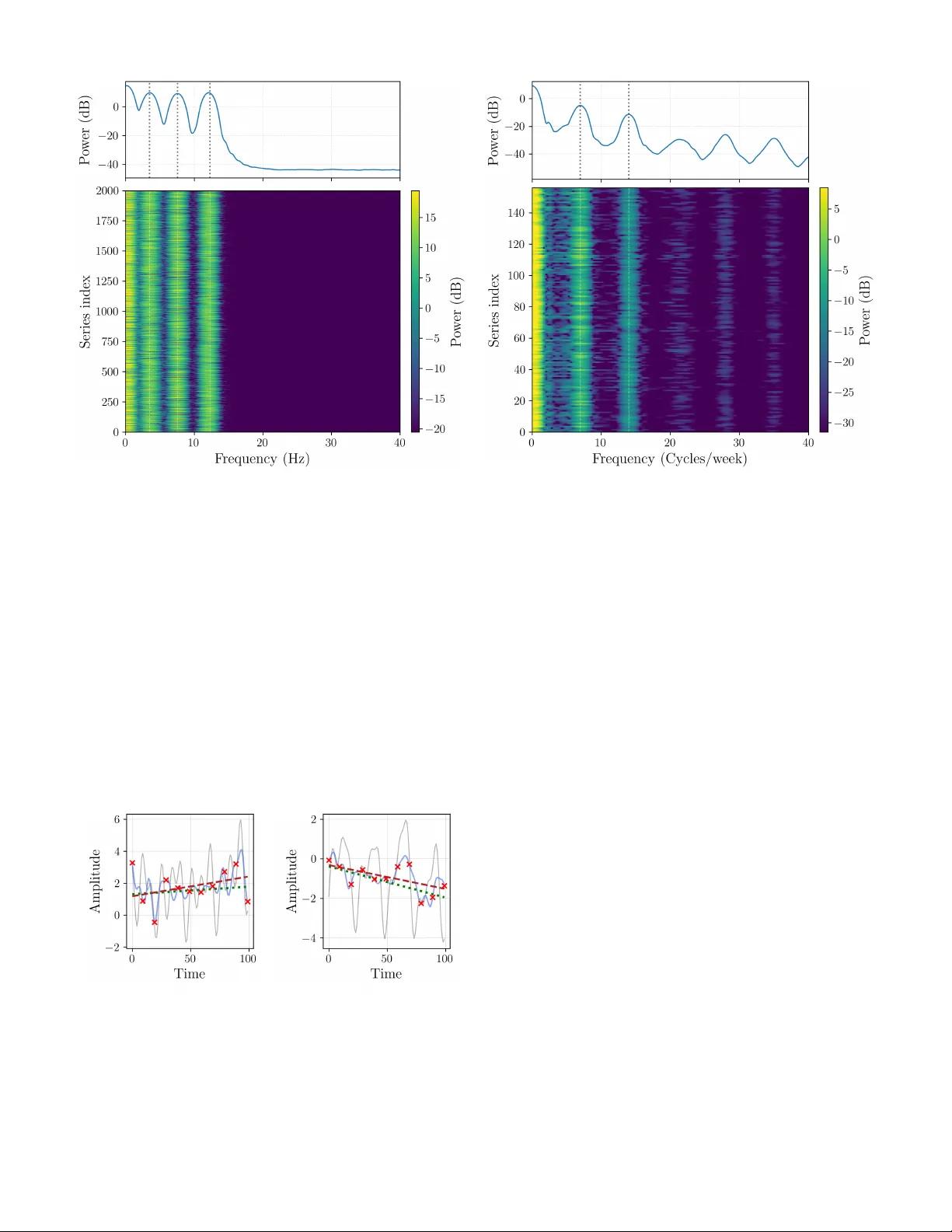
Prior -Informed Neural Network Initialization: A Spectral Approach for Function P arameterizing Architectures 1 st David Orlando Salazar T orres, 2 nd Diyar Altinses, 3 rd Andreas Schwung Department of Automation T ec hnology and Learning Systems South W estphalia University of Applied Sciences Soest, Germany salazartorres.davidorlando, altinses.diyar , schwung.andreas@fh-swf.de Abstract —Neural network ar chitectures designed f or function parameterization, such as the Bag-of-Functions (BoF) frame- work, bridge the gap between the expressivity of deep learning and the interpretability of classical signal processing . Howe ver , these models are inherently sensitive to parameter initializa- tion, as traditional data-agnostic schemes fail to captur e the structural properties of the tar get signals, often leading to suboptimal con vergence. In this work, we propose a prior - informed design strategy that leverages the intrinsic spectral and temporal structur e of the data to guide both network initialization and architectural configuration. A principled methodology is introduced that uses the Fast Fourier T ransf orm to extract dominant seasonal priors, informing model depth and initial states, and a residual-based regression approach to parame- terize trend components. Crucially , this structural alignment enables a substantial reduction in encoder dimensionality without compromising reconstruction fidelity . A supporting theoretical analysis pr ovides guidance on trend estimation under finite- sample regimes. Extensive experiments on synthetic and real- world benchmarks demonstrate that embedding data-driven priors significantly accelerates con vergence, reduces performance variability across trials, and impr oves computational efficiency . Overall, the proposed framework enables more compact and interpr etable ar chitectures while outperforming standard initial- ization baselines, without altering the core training procedur e. Index T erms —Neural network initialization, Bag-of-Functions, time series decomposition, spectral analysis, interpretable ma- chine learning, function parameterization I . I N T RO D U C T I O N Neural networks hav e achiev ed remarkable success across a wide range of domains, including computer vision [1], natural language processing [2], and signal modeling [3], [4]. Their ability to approximate complex nonlinear relationships has made them a cornerstone of modern machine learning. Howe ver , despite their expressiv e power , neural networks re- main inherently sensiti ve to stochastic factors during training, particularly to the initialization of their parameters [5], [6]. The choice of initial weights plays a critical role in shaping the optimization landscape, directly influencing con vergence speed, stability , and final performance. W eight initialization has therefore long been recognized as a key component of effecti ve neural network training. Poor initialization can lead to vanishing or exploding gradients, slow conv ergence, or unstable optimization dynamics [7]. Classical initialization schemes such as Xavier or Kaiming He were developed under assumptions tailored to con ventional deep architectures and specific activ ation functions, aiming to preserve acti vation v ariance across layers. These methods have prov en highly effecti ve for a broad class of tasks, including image classification and language modeling [8]. Howe ver , modern neural architectures designed for function parameterization, such as those emplo yed in the BoF frame- work, exhibit structural properties that deviate significantly from these assumptions. In such models, the network outputs directly parameterize families of mathematical functions used to reconstruct signals, rather than abstract latent features. As a result, traditional data-agnostic initialization strategies fail to account for the statistical and intrinsic structure of the underlying signals, often leading to slo w con ver gence, unstable training beha vior , and lar ge performance variability across runs [4]. While sev eral w orks ha ve explored alternative initializa- tion strategies based on expert knowledge or domain-specific heuristics to mitigate these issues, these approaches often lack generality . The y typically require substantial manual tuning to bridge the gap between the model and the data, limiting their scalability across div erse domains [9]. In this paper , we propose a data-driv en and prior-informed design strategy for neural networks within the Bag-of- Functions frame work. Rather than treating initialization as an isolated optimization heuristic, our approach leverages intrinsic spectral and temporal properties of the data to guide both network initialization and architectural configuration. Specifically , we employ the F ast Fourier Transform (FFT) to extract dominant seasonal components, which define the number of residual stages and initialize the respective encoder networks, alongside a residual-based regression strategy to parameterize trend components. By explicitly encoding these priors into both the architecture and the initial parameteriza- tion, the proposed method ef fectiv ely steers the optimization process from the start of training. This principled structural alignment not only stabilizes training but also enables a substantial reduction in encoder dimensionality without sacrificing reconstruction accuracy . As demonstrated through theoretical analysis and extensi ve empirical e valuation, the proposed frame work leads to faster con vergence, reduced parameter drift, improved computational efficienc y , and more consistent performance across trials. The main contrib utions of this paper are summarized as follows: • W e introduce a data-driv en design framew ork for Bag- of-Functions architectures, in which intrinsic spectral and temporal priors explicitly guide both weight initialization and architectural configuration. • W e show that aligning model capacity with intrinsic data complexity leads to a more ef ficient allocation of repre- sentational resources, eliminating unnecessary depth and enabling significantly more compact encoders without sacrificing reconstruction fidelity . • W e provide analytical support for the proposed frame- work, establishing reliability guarantees for spectral de- composition and residual-based trend estimation under finite-sample regimes. • Through extensiv e e xperiments on synthetic and real- world datasets, we demonstrate that the proposed ap- proach accelerates conv ergence, reduces parameter drift and performance variability across trials, and consistently outperforms state-of-the-art approaches. The remainder of this paper is organized as follows. Section II revie ws prior work on function parameterization and data- driv en initialization. Section III establishes the background on the BoF architecture and formally defines the initialization problem. Section IV introduces the general informed initializa- tion frame work, while Section V details the spectral estimation strategy using the Fourier spectrum. Section VI provides a theoretical analysis of sample size requirements and finite- sample guarantees for regression in noisy time series. Section VII describes the e xperimental setup, dataset details, and presents the comprehensive ev aluation results against state-of- the-art benchmarks. Finally , Section VIII concludes the paper and discusses future research directions. I I . R E L A T E D W O R K In this section, we revie w prior work rele vant to our proposed approach. W e first discuss adv ancements in function parameterization, with a particular focus on neural network- based models such as the Bag-of-Functions framew ork. W e then revie w existing techniques for informed initialization, emphasizing methods that incorporate prior knowledge to improv e neural network optimization. A. Function P ar ameterization Function parameterization constitutes a foundational paradigm for representing and modeling comple x signals and temporal processes, enabling tasks such as forecasting, reconstruction, and anomaly detection [10]. Classical approaches, including polynomial bases and Fourier series, rely on fix ed functional forms, which often lack the fle xibility required to capture complex, nonstationary patterns in real- world data. Neural networks, by contrast, hav e emerged as powerful tools for implicit function parameterization, of fering significantly enhanced expressi ve capacity [11]. Prominent neural architectures for time series modeling include N-BEA TS, which employs a deep residual structure to perform basis expansion. In its interpretable configuration, N- BEA TS explicitly decomposes signals into trend and seasonal components [12]. Related approaches, such as Implicit Neural Representations (INRs), learn continuous functional mappings directly from data [13]. Despite their expressi veness, these models are typically initialized using standard, architecture- dependent schemes rather than priors deri ved from the intrinsic properties of the signals. A particularly relev ant line of work is the BoF framew ork, which has been extensi vely explored for interpretable signal modeling. Early contributions employed BoF representations to generate synthetic time series for pre-training autoencoders in data-scarce regimes [14]. Subsequent extensions introduced probabilistic generativ e formulations, including ITF-V AE and ITF-GAN, enabling the synthesis and manipulation of high- fidelity time series via latent functional representations [15], [16]. Beyond generative modeling, BoF architectures ha ve been adapted for resampling multi-resolution signals, handling variable-length sequences, and robust unsupervised data impu- tation [17], [18]. Recent work has further in vestigated architectural refine- ments within the BoF paradigm, including sparse parame- ter representations, flexible acti vation functions, and encoder design optimizations aimed at improving efficienc y and ex- pressivity [4], [19]. Collectively , these studies demonstrate the versatility and interpretability advantages of BoF-based models across a wide range of signal processing applications. Despite these advances, most function-parameterizing archi- tectures remain largely decoupled from the empirical structure of the signals they aim to model. While architectural refine- ments and inducti ve biases, such as periodic activ ations in im- plicit neural representations [20] or Fourier feature mappings to mitigate spectral bias [21], have significantly improved e x- pressivity , these approaches encode generic assumptions about signal structure rather than priors extracted from individual data instances. As a result, the incorporation of instance- specific structural information into the ov erall model design remains just as limited as the data-based complexity control on the number of function to be parameterized. This limitation highlights an unexploited opportunity to lev erage classical signal analysis techniques, specifically spectral decomposition and trend estimation, not merely as preprocessing steps but as mechanisms to explicitly inform the initialization and configuration of function-parameterizing networks. B. Informed Data-driven Initialization Beyond purely random or architecture-dependent initial- ization schemes, a growing body of work has in vestigated unsupervised, data-driv en strate gies for neural netw ork initial- ization. The central idea is to extract informativ e priors from the training data in order to pro vide a more fa vorable starting point for optimization, thereby accelerating conv ergence and improving final solution quality [22]. Sev eral approaches lev erage statistical or geometric proper- ties of the data. For example, some methods employ clustering techniques such as k-means over candidate weight initial- izations, selecting centroids associated with lower forward- pass error as initialization points [23]. Other techniques use Principal Component Analysis (PCA) to align initial weight vectors with directions of maximal data variance, ensuring early sensiti vity to dominant signal components [24]. While ef- fectiv e in general settings, these approaches are not tailored to architectures whose outputs directly parameterize interpretable functions. In the context of Bag-of-Functions models, recent studies hav e explicitly examined the impact of initialization and demonstrated that aligning parameter distributions with v alid functional ranges improves training stability and con vergence behavior [4]. Howe ver , such strategies typically rely on fixed or manually designed assumptions about parameter statistics, rather than on priors extracted directly from the observ ed signal instances. More broadly , existing data-driv en initialization methods primarily operate at the lev el of statistical distributions or cov ariance structure, largely overlooking intrinsic signal char - acteristics such as dominant spectral components or tempo- ral trends. Moreov er , initialization is typically treated inde- pendently of architectural design choices, leaving open the question of how data-deriv ed priors might jointly inform both the optimization starting point and the allocation of model capacity . Addressing this limitation, by coupling initialization with architecture sizing based on empirically observed spectral and temporal priors, constitutes an open research challenge that the present work seeks to address. I I I . B AC K G R O U N D A N D P RO B L E M F O R M U L A T I O N The Bag-of-Functions frame work is an encoder–decoder architecture designed for the interpretable decomposition of time series into fundamental components such as seasonal- ity , trend, and ev ents [4]. Unlike classic models that learn implicit representations, the BoF approach employs a neu- ral network encoder , E θ , to explicitly map an input signal x i = [ x i ( t 1 ) , . . . , x i ( t T )] ⊤ ∈ R T to a latent vector of parameters z i = E θ ( x i ) . This parameter vector defines a set of analytic basis functions { ϕ a ( t ; z i,a ) } A a =1 , with t = [ t 1 , . . . , t T ] ⊤ , whose linear combination reconstructs the signal through a functional decoder . In this way , the BoF formulation establishes a bridge between the expressi ve capacity of neural networks and the transparency of classical signal models, en- abling the decomposition of complex signals into semantically meaningful components. Building on this formulation, the BoF model employs a residual hierarchy that sequentially isolates these distinct signal components. Each block operates on the residual of the previous block, promoting functional disentanglement and ensuring that each component is represented by its own parameterized basis functions. This residual hierarchy can be extended by stacking multiple BoF stages, each operating on the residual output of the previous one. Such a configuration, referred to as a stacked Bag-of-Functions architecture, allows for progressi ve refinement of the decomposition, enabling the model to capture higher -order interactions or subtle variations across components while preserving interpretability . Formally , the decomposition process is defined by three encoder networks, namely E θ s , E θ t , and E θ e , which infer the parameters of the seasonal, trend, and ev ent components, respectiv ely . Each encoder receives as input the residual of the preceding block, generating latent vectors z s i , z t i , and z e i that parameterize the analytic basis functions used for reconstruction: z s i = E θ s ( x i ) , ˆ x s i = J X j =1 ϕ j ( t ; z s i,j ) , (1) z t i = E θ t ( x i − ˆ x s i ) , ˆ x t i = K X k =1 ϕ k ( t ; z t i,k ) , (2) z e i = E θ e ( x i − ˆ x s i − ˆ x t i ) , ˆ x e i = L X l =1 ϕ l ( t ; z e i,l ) . (3) The overall signal reconstruction is then obtained as ˆ x i = ˆ x s i + ˆ x t i + ˆ x e i . (4) The latent representations z s i , z t i , and z e i provide compact and interpretable parameterizations of each component, captur - ing oscillatory , structural, and transient dynamics, respectively . Concatenating them yields a unified latent encoding of the signal, z i = [ z s i , z t i , z e i ] . (5) The analytical families of basis functions ϕ ( t ; z ) are central to the interpretability of the BoF framework. Each family captures a specific temporal behavior associated with one component of the decomposition. The parameters z inferred by the encoders correspond to the coef ficients or shape factors of these analytic functions, which can be expressed symbolically as a j , the learned counterparts of z i,a for each basis element. Follo wing the taxonomy of [4], sinusoidal and harmonic functions model periodic patterns related to seasonality , poly- nomial and logarithmic forms represent slowly varying trends, and localized kernels such as Gaussian, sigmoidal, or step- like functions describe transient or e vent-related phenomena. Representativ e examples are summarized in T able I. Giv en the parametric nature of the BoF representation, model performance is highly sensitive to the initialization of the encoder weights, θ . Standard initialization schemes, such as Xavier or Kaiming, are inadequate for models whose outputs represent meaningful function parameters rather than abstract feature embeddings. Recent work has addressed this limitation by extending the Kaiming method with a bias term in the final encoder layer, b ( L ) , drawn from a normal distrib u- tion. This modification enables the initial output parameters, T ABLE I: Representati ve basis functions categorized by com- ponent type [4]. The symbolic parameters a j correspond to the learned parameters z i,a inferred by the BoF encoders. Category Function Parameters Seasonality a 1 sin( a 2 t + a 3 ) a 1 , a 2 , a 3 a 1 cos( a 2 t + a 3 ) a 1 , a 2 , a 3 a 1 sinc( a 2 t + a 3 ) a 1 , a 2 , a 3 T rend a 1 a 1 a 1 t a 1 a 1 t 2 + a 2 t a 1 , a 2 a 1 t 3 + a 2 t 2 + a 3 t a 1 , a 2 , a 3 a 1 (1 − e ta 2 ) a 1 , a 2 a 1 ( t + a 2 ) a 3 a 1 , a 2 , a 3 a 1 log( t + a 2 ) a 1 , a 2 Events a 1 step( t, a 2 ) a 1 , a 2 a 1 e − a 2 ( t − a 3 ) 2 a 1 , a 2 , a 3 a 1 tanh( a 2 ( t − a 3 )) a 1 , a 2 , a 3 a 1 sig( a 2 ( t − a 3 )) a 1 , a 2 , a 3 z i at the beginning of training, to be centered around a desired mean µ and variance σ 2 [4]: b ( L ) ∼ N ( µ, σ 2 ) = ⇒ z (0) i ≈ N ( µ, σ 2 ) . (6) The objectiv e is to select the hyperparameters ( µ, σ 2 ) such that this initial distribution approximates the true, underlying parameter distribution of the dataset, denoted P ∗ ( z ) . Howe ver , let H = { S, N in , µ, σ 2 } define the complete set of structural and initialization hyperparameters, where S denotes the num- ber of stacked decomposition stages and N in represents the input dimension (receptive field) of the trend encoders. In current practice, the configuration vector h ∈ H is selected heuristically , independent of the signal properties. This lack of data specificity may lead to structural mismatch or statis- tical inef ficiency , resulting in suboptimal con ver gence or poor alignment between the initial parameter space and the structure of the signals in a giv en dataset D . T o address this limitation, we propose a principled, data- driv en method for determining an improved configuration h ∗ ∈ H by estimating it directly from the dataset. Specifi- cally , we introduce a framew ork that establishes a mapping M : D → H ∗ based on spectral and statistical analysis. W e utilize the cardinality of the dominant spectral modes, |K τ | , to formally deriv e the required number of stages S , while a finite-sample regression analysis determines the minimal input size N in required to bound the estimation v ariance. Concurrently , empirical estimates ( ˆ µ data , ˆ σ 2 data ) are computed to inform the weight initialization. This yields a model topology and state explicitly tailored to the intrinsic structure of the data, pro viding a more robust and efficient starting point for training BoF models. I V . I N F O R M E D I N I T I A L I Z A T I O N F R A M E W O R K The proposed framework extends the Bag-of-Functions ar- chitecture through a data-informed strategy that gov erns both design and initialization. As illustrated in Figure 1, extracted seasonal and trend statistics serve as priors that e xplicitly determine the structural topology by defining the number of decomposition stages and the trend encoder input sizes, while simultaneously guiding the initialization of the encoder weights. This alignment ensures the model is instantiated with properties consistent with the empirical data structure, crucially enabling the subsequent training phase to resolve the complex nonlinear temporal behaviors and event-dri ven variations that cannot be represented by purely spectral or linear methods. Fig. 1: Overvie w of the proposed data-informed frame- work. Extracted seasonal and trend statistics serve as priors that jointly determine the architectural topology , including stage depth and input dimensions, and initialize the Bag-of- Functions encoder weights to align the model with the data structure before training. Formally , the framew ork operates sequentially to establish a mapping from the dataset D to the improved configuration H ∗ . First, spectral analysis via the Fast Fourier T ransform (FFT) identifies the set of dominant frequencies K ( τ ) . The cardinal- ity of this set, |K ( τ ) | , directly informs the required number of stages S , while the empirical mean and variance of the corresponding spectral coefficients constitute the initialization statistics, denoted ( ˆ µ data , ˆ σ 2 data ) . These v alues define the data- driv en priors for initializing the seasonal Bag-of-Functions encoder: z (0) s ∼ N ( ˆ µ data , ˆ σ 2 data ) . (7) Subsequently , the trend information is estimated through linear regression applied to the residual signal obtained after removing the identified seasonal components. This analysis yields two critical outcomes regarding both the architec- ture and the optimization state. On the structural front, the estimated residual noise variance ˆ σ 2 ε and the tar get slope tolerance δ are used to deriv e the minimum input dimension N in required for reliable trend estimation, utilizing the finite- sample guarantees deriv ed in Section VI. Concurrently , the empirical statistics of the slope and bias coefficients update the priors ( ˆ µ data , ˆ σ 2 data ) specifically for the trend encoder . This data-driv en alignment ensures that the encoder outputs lie within the valid parameter space of the tar get signals from the first iteration, mitigating the risk of spectral bias or v anishing gradients associated with random initialization. The ov erall procedure for extracting these hyperparameters is summarized in Algorithm 1. The algorithm processes the dataset to deriv e the configuration vector h ∗ , which is then used to instantiate and initialize the Bag-of-Functions archi- tecture. Algorithm 1 Data-Driven Configuration and Initialization Require: Dataset D = { y ( i ) } N i =1 of N time series 1: Identify dominant spectral modes K from dataset D 2: Set number of decomposition stages S ← |K| 3: Initialize empty lists P t ← [] , P s ← [] 4: for i = 1 , . . . , N do 5: Estimate seasonal parameters ˆ θ ( i ) s for modes K 6: Compute seasonal component ˆ s ( i ) ( t ) ← f s ( t ; ˆ θ ( i ) s ) 7: Form residual ˜ y ( i ) ( t ) ← y ( i ) ( t ) − ˆ s ( i ) ( t ) 8: Estimate trend parameters ˆ θ ( i ) t = (ˆ a ( i ) , ˆ b ( i ) ) on ˜ y ( i ) 9: Append ˆ θ ( i ) s to P s and ˆ θ ( i ) t to P t 10: end for 11: Compute input dimension N in from residual statistics 12: Compute empirical priors ( ˆ µ data , ˆ σ 2 data ) from P s and P t 13: Configure and initialize Bag-of-Functions architecture The practical realization of this framew ork relies on trans- lating these statistical priors into concrete architectural and parametric specifications. In the follo wing sections, we treat the Fourier spectrum not merely as a feature extractor , but as a topological blueprint: the distribution of spectral energy rev eals the signal’ s intrinsic multi-resolution structure, ef fec- tiv ely prescribing the hierarchical depth ( S ) based on signal complexity rather than heuristics. Crucially , this analytical foundation acts as a complementary scaffold rather than a substitute; it allo ws the Bag-of-Functions model to bypass the learning of trivial linear components and focus its expressiv e power on resolving the comple x non-stationary dynamics and transient e vents that remain inaccessible to classical methods. Combined with the bias-based initialization adapted from [4], this approach ensures a stable starting state. Accordingly , Sec- tion V details this spectral mapping strate gy , while Section VI establishes the theoretical bounds for stable trend estimation. V . E S T I M A T I N G S E A S O N A L P A R A M E T E R S V I A F O U R I E R S P E C T RU M This section introduces a principled framework for estimat- ing seasonal priors from the frequency domain. The analy- sis identifies dominant periodic components whose empirical statistics are used to initialize the seasonal encoder of the Bag- of-Functions model. Beyond parameter estimation, the spectral distribution of energy re veals the multi-resolution structure of the data, guiding the design of hierarchical seasonal stages. Unlike con ventional Fourier methods, which focus on linear reconstruction, this approach le verages spectral descriptors to inform the initialization and configuration of the BoF architecture, enabling it to e xploit its ability to model nonlinear and ev ent-driven temporal dynamics. A. Spectral Modeling and F r equency Selection T o derive empirical priors for the seasonal encoder , each time series in the dataset is modeled as the superposition of three components: y t = s t + t t + ε t , t = 1 , . . . , n, (8) where s t represents the seasonal component associated with periodic fluctuations, t t denotes the slowly v arying trend, and ε t is additiv e noise. The objective o f this stage is to extract information about s t from the frequency domain, providing a compact summary of the dominant periodic behavior in the data. The spectral content of y t is analyzed using the Discrete Fourier T ransform (DFT), Y ( ω k ) = n X t =1 y t e − 2 π iω k t , ω k = k n , k = 0 , 1 , . . . , n − 1 , (9) whose squared magnitude defines the periodogram, I y ( ω k ) = 1 n | Y ( ω k ) | 2 . (10) The periodogram quantifies the distribution of signal energy across frequencies, enabling the identification of peaks asso- ciated with dominant oscillatory patterns. These frequencies capture the primary components of s t , while the trend t t and noise ε t contribute mainly to the low- and high-frequency regions, respecti vely . T o isolate meaningful periodicities, we employ a relativ e- power thresholding criterion. Let P max = max 0 ≤ k ≤⌊ n/ 2 ⌋ I y ( ω k ) (11) be the maximum spectral po wer, and define a threshold pa- rameter τ ∈ (0 , 1) , typically τ = 0 . 2 . The set of dominant frequencies is then K ( τ ) = { k : I y ( ω k ) ≥ τ P max , 0 ≤ k ≤ ⌊ n/ 2 ⌋} . (12) For each retained frequency ω k ∈ K ( τ ) , the amplitude A k = 2 | C k | and phase ϕ k = arg( C k ) are computed from C k = 1 n Y ( ω k ) . These quantities represent coarse estimates of the seasonal characteristics of the dataset. The empirical distributions of { A k , ω k , ϕ k } across all time series define the statistical priors ( ˆ µ data , ˆ σ 2 data ) , which are used to initialize the bias parameters of the BoF seasonal encoder . Moreov er, the global spectral distribution provides an estimate of ho w many distinct frequency bands are relev ant, offering a data-driven guideline for configuring the number of seasonal stages in stacked BoF architectures. B. Spectral Ener gy Ratio as a Diagnostic Metric T o quantify the informativ eness of the identified frequen- cies, we compute the proportion of signal energy explained by the retained components: ρ spec = P k ∈K ( τ ) | C k | 2 P n − 1 k =0 | C k | 2 . (13) A high value of ρ spec indicates that the time series exhibits strong periodicity , suggesting that the spectral priors are re- liable indicators for encoder initialization. Con versely , a low ρ spec implies weak seasonality , in which case the model relies more heavily on trend and event encoders during training. This measure thus serves as a practical diagnostic tool for ev aluating the spectral richness of the dataset and for adapting the initialization strength of the seasonal stage. The deseason- alized residual obtained after this analysis serves as the input for estimating trend parameters, as described in the follo wing section. V I . S A M P L E S I Z E R E QU I R E M E N T S F O R L I N E A R R E G R E S S I O N I N N O I S Y T I M E S E R I E S In order to capture the underlying trend across the dataset, we apply a linear regression model to each time series sample. This procedure provides a simple and interpretable way to characterize the local direction and strength of change, which can then be aggreg ated or used for the informed initialization of the Bag-of-Functions architecture. While many time series exhibit additional seasonal or cyclical patterns, the linear regression applied at the segment lev el serves as a first-order approximation of the local trend, effecti vely separating long- term drift from random noise. Since the number of regressions to be performed can be e xtremely large, it becomes crucial to understand ho w many observations within each segment are actually required to obtain reliable parameter estimates. In particular, we are interested in quantifying the minimum segment length needed to estimate the slope and bias with a prescribed level of accuracy and confidence, thereby providing a principled trade- off between statistical precision and computational or data- collection cost. Moreov er, this analysis also offers practical guidance for model design: the minimum segment length directly translates into the temporal windo w size required by the trend encoder , defining the effectiv e receptive field of the neural network necessary to capture stable linear dynamics in noisy en vironments. A. Model Setup W e consider a time series segment of length n with obser- vations y i = a + b t i + ε i , i = 1 , 2 , . . . , n, (14) where a is the bias, b is the slope, t i denotes the time index (assumed equally spaced), and ε i are stochastic noise terms with zero mean. Note that we subtract the seasonal components from Equation (8) as previously defined. The ordinary least squares (OLS) estimator ˆ β = ( ˆ a, ˆ b ) ⊤ minimizes the squared residuals and admits the closed form ˆ β = ( X ⊤ X ) − 1 X ⊤ y , (15) where X is the design matrix with rows (1 , t i ) . A central quantity in this analysis is the centered sum of squares of the time indices, S xx = n X i =1 ( t i − ¯ t ) 2 , ¯ t = 1 n n X i =1 t i . (16) This term quantifies how widely the design points are dis- tributed along the time axis. A larger spread (higher S xx ) leads to more precise estimates of the slope b , since the regression has greater lev erage to separate signal from noise. When the time indices are equally spaced, i.e., t i = i for i = 1 , . . . , n , the mean time index is ¯ t = 1 n n X i =1 i = n + 1 2 . (17) Substituting this into the definition of S xx giv es S xx = n X i =1  i − n + 1 2  2 = n X i =1 i 2 − n  n + 1 2  2 . (18) Using the standard identity for the sum of squares, n X i =1 i 2 = n ( n + 1)(2 n + 1) 6 , (19) and substituting into Equation (18) yields S xx = n ( n + 1)(2 n + 1) 6 − n  n + 1 2  2 = n ( n 2 − 1) 12 . (20) For large n , this expression scales as S xx ∼ n 3 12 , indicating that the ef fectiv e spread of the design and, consequently , the statistical leverage of the regression, increase cubically with the number of observ ations. This property directly determines the rate at which the slope estimator con ver ges in the subse- quent analysis. The closed-form expression for S xx deriv ed here will serve as the foundation for quantifying the variance and concentration properties of the slope estimator in the ne xt subsection. B. Estimation Err or of the Slope From the general OLS solution ˆ β = ( X ⊤ X ) − 1 X ⊤ y and the linear model y = X β + ε , we can express the estimation error as ˆ β − β = ( X ⊤ X ) − 1 X ⊤ ε. (21) For the slope component, corresponding to the second entry of ˆ β , this giv es ˆ b − b = e ⊤ 2 ( X ⊤ X ) − 1 X ⊤ ε, (22) where e 2 = (0 , 1) ⊤ selects the slope coordinate. Using the structure of the design matrix X =    1 t 1 . . . . . . 1 t n    , and applying the standard OLS algebra, one obtains the explicit scalar form ˆ b = P n i =1 ( t i − ¯ t ) y i P n i =1 ( t i − ¯ t ) 2 . (23) Substituting y i = a + bt i + ε i into this expression yields ˆ b − b = P n i =1 ( t i − ¯ t )( a + bt i + ε i ) S xx − b (24) = a P n i =1 ( t i − ¯ t ) + b P n i =1 ( t i − ¯ t ) 2 + P n i =1 ( t i − ¯ t ) ε i S xx − b. (25) The first term vanishes because P i ( t i − ¯ t ) = 0 , and the second term cancels with b after di viding by S xx . Thus we obtain the key relation ˆ b − b = 1 S xx n X i =1 ( t i − ¯ t ) ε i . (26) Equation (26) shows that the slope estimation error is a weighted a verage of the noise terms, where the weights depend linearly on the centered time indices. Observations farther from the mean time point contribute more heavily to the estimate, which intuitiv ely explains why a wider time span yields a more stable slope estimate. Assuming that the noise terms are independent with E [ ε i ] = 0 and V ar( ε i ) = σ 2 , the v ariance of the slope estimator follows directly: V ar( ˆ b ) = V ar 1 S xx n X i =1 ( t i − ¯ t ) ε i ! (27) = 1 S 2 xx n X i =1 ( t i − ¯ t ) 2 V ar( ε i ) (28) = σ 2 S xx . (29) Substituting the equidistant design result S xx = n ( n 2 − 1) / 12 giv es the asymptotic behavior V ar( ˆ b ) ∼ 12 σ 2 n 3 , n → ∞ . (30) Hence, the standard deviation of ˆ b decreases at the rate n − 3 / 2 —a much faster con vergence than the usual n − 1 / 2 rate obtained when estimating a mean. This acceleration arises because slope estimation benefits from the cubic increase in the time-index spread, which amplifies the information g ained from additional observations. C. Concentration Bounds and F inite-Sample Guarantees While v ariance calculations describe asymptotic precision, they do not quantify the reliability of estimates for finite sample sizes. T o obtain non-asymptotic guarantees, we study the distrib ution of the slope estimator under sub-Gaussian noise assumptions. Assumption VI.1. The noise variables ε i ar e independent, center ed, and sub-Gaussian with variance proxy σ 2 , i.e., E [ e λε i ] ≤ exp  λ 2 σ 2 2  , ∀ λ ∈ R . (31) This assumption includes the Gaussian case b ut also accom- modates other light-tailed distributions. Theorem VI.1. Under Assumption VI.1, for any tolerance level δ > 0 , P ( | ˆ b − b | > δ ) ≤ 2 exp  − δ 2 S xx 2 σ 2  . (32) Pr oof. From Equation (26), the slope estimation error can be written as ˆ b − b = 1 S xx n X i =1 ( t i − ¯ t ) ε i = n X i =1 w i ε i , (33) where the weights w i = ( t i − ¯ t ) /S xx are deterministic and satisfy P w 2 i = 1 /S xx . By the standard closure property of sub-Gaussian v ariables, any weighted sum of independent sub-Gaussian terms remains sub-Gaussian. In particular , if each ε i is sub-Gaussian with variance proxy σ 2 , then the sum Z = n X i =1 w i ε i is sub-Gaussian with variance proxy σ 2 Z = σ 2 n X i =1 w 2 i = σ 2 S xx . By definition of sub-Gaussianity , for any u > 0 , P ( | Z | > u ) ≤ 2 exp  − u 2 2 σ 2 Z  = 2 exp  − u 2 S xx 2 σ 2  . (34) Finally , substituting back Z = ˆ b − b and setting u = δ yields the stated concentration inequality . ■ Theorem VI.1 provides a direct link between the design spread S xx , the noise lev el σ 2 , and the desired accuracy δ . The larger the effecti ve spread S xx , the tighter the estimator concentrates around the true slope. A practical corollary gives an explicit sample-size require- ment. T o ensure that | ˆ b − b | ≤ δ with probability at least 1 − α , it suffices that S xx ≥ 2 σ 2 log(2 /α ) δ 2 . (35) In the equidistant case t i = i , we hav e S xx = n ( n 2 − 1) / 12 ≈ n 3 / 12 , and substituting into Equation (35) giv es n ≥  24 σ 2 log(2 /α ) δ 2  1 / 3 . (36) Hence, the required segment length gro ws only as the two- thirds power of the signal-to-noise ratio ( σ /δ ) . This is con- siderably milder than the quadratic scaling typical of mean estimation, reflecting the higher efficienc y of slope estimation due to the cubic growth of S xx . For illustration, consider a target tolerance δ = 0 . 1 , con- fidence lev el 95% ( α = 0 . 05 ), and noise variance σ 2 = 1 . Substituting into Equation (36) giv es n ≥  24 ln(40) 0 . 1 2  1 / 3 ≈ 20 . 7 . (37) Thus, a segment length of n = 21 equidistant observations is sufficient to guarantee the desired estimation accuracy under independent Gaussian noise. This provides a practical lower bound for the temporal window size required by the trend encoder in the Bag-of-Functions framew ork. D. Bias Estimation W e now turn to the bias estimator ˆ a . Unlike the slope, the bias does not directly benefit from the design spread of the time indices. Instead, it primarily reflects the a verage noise lev el across the segment, which leads to a different scaling behavior . From the standard OLS relation ˆ a = ¯ y − ˆ b ¯ t , substituting y i = a + bt i + ε i giv es ˆ a − a = 1 n n X i =1 ε i − ( ˆ b − b ) ¯ t. (38) The first term corresponds to the sample mean of the noise, while the second term captures the propagated uncertainty from the slope estimation, scaled by the mean of the time indices. In the equidistant case, these two components are uncorrelated, and thus their variances add. Assuming independent errors with variance σ 2 , we obtain V ar(ˆ a ) = σ 2  1 n + ¯ t 2 S xx  . (39) The first term arises from the sample mean variance V ar( ¯ ε ) = σ 2 /n , while the second follows from V ar( ˆ b − b ) = σ 2 /S xx , scaled by ¯ t 2 . Cross-terms vanish due to the orthogonality of the OLS decomposition. For equidistant time indices t i = i , we have ¯ t = ( n + 1) / 2 and S xx ∼ n 3 / 12 . Substituting these expressions yields V ar(ˆ a ) ∼ σ 2 n , n → ∞ . (40) Thus, the bias estimator conv erges at the classical n − 1 / 2 rate, identical to the sample mean. Unlike the slope, it does not benefit from the cubic increase of S xx , since it captures the baseline lev el rather than the rate of change. From a practical standpoint, this distinction is relev ant. T o estimate the slope within tolerance δ , one needs on the order of n ≍ ( σ /δ ) 2 / 3 observations, whereas for the bias the requirement increases to n ≍ ( σ /δ ) 2 . Hence, achie ving a high- precision bias estimate is significantly more demanding than estimating the slope. E. Implications for Ar chitectur e Design While the asymptotic properties of the ordinary least squares estimator are classical results in statistical theory , their ap- plication within the context of neural network design offers an alternativ e to the heuristic selection of hyperparameters. T ypically , the input size of a trend encoder is determined via costly grid searches or arbitrary rule-of-thumb choices. The deriv ation provided in Theorem VI.1 establishes a direct analytical link between the physical properties of the signal (noise-to-slope ratio) and the structural requirements of the architecture. A critical insight from this analysis is the disparity in con vergence rates between the slope ( ∼ n − 3 / 2 ) and the bias ( ∼ n − 1 / 2 ). In the context of the Bag-of-Functions architecture, the primary goal of the trend encoder is to capture the dynamics of the signal, represented by the slope, rather than its absolute baseline lev el. The cubic scaling of the design spread S xx implies that the encoder can reliably learn local deriv a- tiv es with relati vely compact temporal windo ws. F or instance, the derived bound suggests that a window of approximately n ≈ 20 samples is suf ficient to stabilize the gradient estimation ev en under significant noise ( σ ≈ 1 ), whereas relying on bias con vergence would require significantly larger inputs. This theoretical finding v alidates the ef ficiency of the pro- posed framework: by allowing the linear regression layer to focus on the rapidly con verging slope component, we can minimize the dimensionality of the input layer N in without sacrificing precision. The slo wer-con verging bias component acts merely as a bias term, which neural networks are natu- rally equipped to correct through their internal bias weights during the training phase via backpropagation. Consequently , Equation (36) serves as a formal lower bound for the receptive field size, ensuring that the model is instantiated with suf ficient informational capacity to distinguish trends from noise prior to any optimization. V I I . E V A L U A T I O N This section presents the experimental ev aluation of the proposed frame work. The analysis is structured in three parts. First, the datasets used for training and validation are de- scribed, including a controlled synthetic dataset and two real- world datasets representing distinct signal domains. Next, the experimental setup outlines the implementation details, param- eter configurations, and ev aluation protocol employed. Finally , the results section reports both quantitative and qualitativ e findings, highlighting the effecti veness of the prior-informed initialization and the interpretability achie ved by the Bag-of- Functions architecture. The ev aluation further demonstrates how data-deri ved information guides key architectural choices, such as the number of stages and the encoder window size, thereby achieving a principled balance between interpretability and efficienc y . A. Dataset T o validate the proposed data-informed strategy for archi- tectural design and initialization, we employ both synthetic and real-world benchmarks. These datasets encompass div erse temporal dynamics, enabling a systematic ev aluation of ho w extracted spectral and trend priors effecti vely guide the instan- tiation of the BoF encoders. The synthetic dataset was constructed to provide a reference benchmark with known spectral and temporal parameters. Each signal y i ( t ) combines periodic components, a linear trend, and a localized transient ev ent, modeled as y i ( t ) = 3 X k =1 A i,k sin  2 π f i,k t + ϕ i,k  + ( α i, 0 + α i, 1 t ) + β i exp  − ( t − µ i ) 2 2 σ 2 e  + ε i ( t ) . (41) The spectral parameters are drawn independently , with frequencies f i,k normally distributed around centers { 3 . 5 , 7 . 5 , 12 . 0 } Hz, amplitudes A i,k following a positiv e normal distribution, and phases ϕ i,k uniform in [0 , 2 π ] . Both trend and event parameters are sampled from bounded uniform distrib utions to introduce variability , while the additiv e noise follows ε i ( t ) ∼ N (0 , 0 . 01 2 ) . Comprising N = 2000 signals sampled at T = 100 equidistant points ov er the normalized interv al t ∈ [0 , 1] , this dataset enables a direct quantitativ e ev aluation of the estimated priors against the known ground truth. T o complement this synthetic benchmark, we utilize two real-world datasets representing div ergent temporal challenges. The first, the PJM Interconnection dataset (1998–2001), cap- tures macro-scale grid dynamics through hourly demand records partitioned into weekly segments to isolate recurrent consumption patterns. The second comprises thermal power plant (TPP) output from a district heating network, sampled at hourly intervals between 2016 and 2020. By focusing on the winter subset of the TPP data, we isolate the prominent periodic and trend components inherent to heating demand, allowing the framew ork to demonstrate its ability to extract meaningful architectural priors across div erse and complex empirical domains. B. Experimental Setup T o assess the impact of the extracted priors on both the architectural design decisions and the parameter initialization strategies, we benchmark four distinct configurations of the Bag-of-Functions network. The first v ariant, denoted as BoF , serves as the domain-agnostic baseline where the encoders are instantiated using standard def ault initialization schemes, representing a scenario dev oid of any specific structural pri- ors. The second v ariant, Heuristics BoF (H-BoF), adopts the initialization philosophy proposed in [4]; ho wev er , while this approach utilizes specific heuristics for initialization, it remains constrained to a fixed architecture that does not incorporate design decisions deriv ed from the dataset’ s specific characteristics. Moving tow ard structurally informed config- urations, the Informed BoF (I-BoF) architecture extends this initialization strategy by replacing generic heuristics with data- driv en values. Crucially , this variant lev erages the spectral analysis to dynamically determine the number of stages of the model and to initialize the seasonal encoders, while the trend component retains a standard configuration. Finally , the In- formed T rend BoF (IT -BoF) represents the complete proposed framew ork where the architecture is fully adapti ve: the depth is defined by the frequency analysis, and the trend encoder input size is dimensioned according to the residual trend volatility . Furthermore, this network is fully initialized with both the spectral seasonal priors and the OLS-deri ved trend priors, ensuring the optimization starts in close proximity to the true signal parameters. T o account for the inherent stochasticity of weight initialization and the optimization landscape, we ex ecuted 10 independent training trials for each dataset-model pair using distinct random seeds. All models were trained using the Adam optimizer with a learning rate of η = 1 × 10 − 3 and a batch size of B = 16 , gov erned by a Mean Squared Error (MSE) loss function with an early stopping mechanism to prev ent overfitting. T o ev aluate the computational efficiency and practical suit- ability of the proposed architectures, we conducted a standard- ized benchmarking protocol on a workstation equipped with an Intel Core i7-11700 CPU, 64 GB RAM, and an NVIDIA R TX 5000 GPU. All models were implemented in PyT orch, and computational complexity was estimated using the thop library . Inference performance was measured under controlled conditions using real input samples from the test sets to ensure representativ e runtime behavior . C. Data-Driven Prior Extr action and Arc hitecture Configura- tion W e apply the prior extraction frame work to the synthetic and real-world datasets in order to instantiate the Bag-of-Functions architecture before training. The objectiv e is twofold: (i) to deriv e empirical priors for encoder initialization, and (ii) to determine the architectural depth and trend encoder input size directly from data. Spectral estimation is first applied to the synthetic dataset described in section VII. Figure 2 reports the average pe- riodogram and the spectral heatmap across all N = 2000 samples. Applying the relativ e-power thresholding criterion ( τ = 0 . 2 ) identifies three dominant modes at 3 . 48 , 7 . 56 , and 12 . 29 Hz, closely matching the ground-truth frequencies. These components account for a cumulative spectral energy ratio of ρ spec = 0 . 873 , indicating strong periodic structure. Accordingly , the BoF architecture is instantiated with |K| = 3 stages, each initialized using the empirical statistics of the corresponding spectral band. Follo wing seasonal e xtraction, a coarse deseasonalization is performed to estimate trend priors. As illustrated in Figure 3, Fig. 2: Spectral analysis of the synthetic dataset used for prior extraction. The a verage periodogram identifies dominant modes at 3 . 48 Hz, 7 . 56 Hz, and 12 . 29 Hz, complemented by the spectral heatmap across all N = 2 , 000 samples. The cumulativ e energy ratio reaches ρ spec = 0 . 873 by combining these three identified modes. the remov al of dominant harmonics exposes the underlying drift, enabling a reliable estimation of the residual noise v ari- ance. Using the finite-sample bound derived in Equation (36) with tolerance δ = 0 . 2 , the resulting stability criterion yields an optimal trend input size of n opt = 11 . These observations are selected equidistantly to maximize the design spread S xx , yielding accurate slope estimates while reducing the input dimensionality by 89% compared to a full-window approach. Fig. 3: V isual validation of the trend estimation on two dataset samples. The plots display the input signal (gray), the deseasonalized input (blue), and the ground truth trend (green dotted). The red markers indicate the specific observations selected for the OLS re gression, yielding the estimated trend (red dashed). Fig. 4: Spectral analysis of the PJM Hourly dataset used for prior extraction. The a verage periodogram identifies dominant modes at 6 . 97 and 13 . 99 cycles/week, while the accompanying spectral heatmap displays the energy distrib ution across all 156 samples. The cumulativ e energy ratio reaches ρ spec = 0 . 960 by combining the two identified dominant modes. The same procedure is applied to the PJM Hourly and Thermal Power Plant (TPP) datasets. For PJM, using a weekly window ( W = 168 ), spectral analysis identifies tw o dominant harmonics at 6 . 97 and 13 . 99 cycles/week, as illustrated in Figure 4, capturing ρ spec = 0 . 960 of the oscillatory energy . Low-frequenc y components are attributed to trend behavior and handled by the linear encoder . Consequently , a two-stage architecture is sufficient. In contrast, the TPP dataset e xhibits a richer spectral struc- ture (Figure 5), with four significant modes at 1 . 42 , 6 . 95 , 14 . 00 , and 21 . 20 cycles/week. Notably , the low-frequency component at 1 . 42 c ycles/week contrib utes 21 . 8% of the total energy and therefore requires explicit modeling as a seasonal stage. The resulting configuration adopts |K| = 4 , achieving near-complete spectral coverage ( ρ spec = 0 . 991 ). T rend priors are estimated from the deseasonalized residuals for both datasets. As shown in Figure 6, the smooth resid- ual structure of PJM leads to a compact configuration with n opt = 3 , whereas the higher volatility of the TPP residuals requires n opt = 13 to satisfy the same stability tolerance of δ = 0 . 1 ( 10% ). Despite these dif ferences, both cases achieve substantial reductions in trend input dimensionality ( > 90% ) while preserving estimation reliability . T able II summarizes the resulting data-dri ven configura- tions. These parameters specify the BoF architecture before training, determining its depth, frequency initialization, and Fig. 5: Spectral analysis of the Thermal Po wer Plant dataset used for prior e xtraction. The average periodogram identifies distributed dominant modes at 1 . 42 , 6 . 95 , 14 . 00 , and 21 . 20 cycles/week, complemented by the spectral heatmap across all 1000 samples. The cumulati ve energy ratio reaches ρ spec = 0 . 991 by combining the four identified modes. (a) PJM Hourly (b) Thermal Po wer Plant Fig. 6: T rend input configuration based on deseasonalized residuals. The blue lines represent the signal proxy obtained by removing the detected harmonics K . The red markers indicate the n opt equidistant observ ations selected to maximize stability , dimensioned according to the estimated residual volatility . trend encoder input size. The extracted priors serve as in- formed starting points rather than fix ed constraints, allo wing the network to refine these estimates during optimization and capture non-linear dynamics beyond the resolution of classical spectral and linear models. W ith the architectural topology and initialization states explicitly defined, we proceed to the empirical v alidation. The following section quantifies the practical impact of these data- driv en priors on training dynamics, comparing the con vergence speed and final accuracy of the proposed strategy against standard paradigms. D. Results This section reports the empirical ev aluation of the pro- posed frame work. W e first analyze optimization beha vior on a synthetic dataset, where ground-truth structure is known. W e then assess generalization performance on the two real- world datasets, followed by an e valuation of computational efficienc y . 1) V alidation on Synthetic Data: The synthetic dataset enables a controlled analysis of how structural priors af fect optimization stability and parameter con vergence. Figure 7 summarizes the final training and testing MSE distributions ov er 10 independent runs per architecture. Fig. 7: Distribution of the final MSE loss on the training (left) and testing (right) sets. The results summarize 10 independent trials for each of the four ev aluated architectures. Reported values represent the a verage loss at the conv erged state. W ithin each box, the solid orange and dashed green lines denote the median and the mean, respectiv ely . The informed architectures (I-BoF and IT -BoF) achiev e the lowest reconstruction error with minimal variance. IT -BoF attains a test MSE of 0 . 0220 ± 0 . 0033 , statistically comparable to I-BoF ( 0 . 0198 ± 0 . 0034 ), despite its reduced trend dimen- sionality . In contrast, the baseline BoF exhibits significantly higher error ( 0 . 7633 ± 0 . 1091 ). Heuristic initialization (H- BoF) improv es performance ( 0 . 1937 mean MSE) but remains less stable. Overall, informed initialization reduces error by approximately 97% relative to the baseline, confirming that structural priors effecti vely stabilize the optimization. T o examine con vergence beha vior, Figure 8 shows the loss trajectories of the best-performing trial per architecture. T ABLE II: Data-Driv en Configuration and Initialization Priors. Consolidated architectural parameters deriv ed from the two- stage diagnostic process. The table segre gates the hyperparameters obtained from spectral decomposition (Seasonal Priors) and residual analysis (T rend Priors). Dataset W in. ( W ) Frequency Analysis (Seasonal Priors) T rend Analysis (T rend Priors) Ratio ( ρ ) Depth Mode Initialization ( K ) Noise ( ˆ σ ) Input ( n opt ) Synthetic 100 0.873 3 [3 . 48 , 7 . 56 , 12 . 29] Hz 0.850 11 PJM Hourly 168 0.960 2 [6 . 97 , 13 . 99] cycles/win 0.048 3 Thermal Plant 168 0.991 4 [14 . 00 , 6 . 95 , 1 . 42 , 21 . 20] cycles/win 0.486 13 Fig. 8: Loss trajectories of the best-performing trial for each architecture. The solid lines represent the moving av erage, while the lighter shaded regions indicate batch volatility . Although all models exhibit relatively high initial errors, the informed variants start with a substantially lower loss. While the baseline BoF con verges slo wly and H-BoF sho ws moderate improv ement, both I-BoF and IT -BoF rapidly reach low-error regimes within early iterations. This confirms that data-driv en priors substantially reduce optimization effort, a benefit that IT -BoF preserves despite its compact trend representation. Figure 9 reports the cumulativ e parameter displacement during training. Fig. 9: Evolution of the parameter displacement during training for the best-performing trial of each architecture. Solid lines represent moving av erages, while shaded regions indicate batch-wise variability . The baseline BoF undergoes large and sustained param- eter shifts, whereas informed architectures stabilize quickly after a brief adjustment phase. IT -BoF exhibits the smallest ov erall displacement, indicating that informed dimensionality reduction not only preserves accuracy but further constrains parameter drift, leading to more stable learning dynamics. 2) Generalization to Real-W orld Scenarios: W e next ev al- uate generalization on two real-world datasets: PJM electricity demand and the Thermal Po wer Plant (TPP) dataset. T able III reports reconstruction performance av eraged o ver 10 indepen- dent trials. T ABLE III: Reconstruction performance on real-world bench- marks. The table reports the Mean Squared Error for the training and testing partitions across the PJM and Thermal Power Plant (TPP) datasets. Results are averaged over ten independent trials per architecture, and the best performance per dataset is highlighted in bold. T raining MSE Dataset BoF H-BoF I-BoF IT -BoF PJM 0 . 0116 ± 0 . 0005 0 . 0066 ± 0 . 0026 0 . 0060 ± 0 . 0007 0 . 0046 ± 0 . 0008 TPP 0 . 4423 ± 0 . 0178 0 . 1957 ± 0 . 0431 0 . 1715 ± 0 . 0025 0 . 1755 ± 0 . 0043 T esting MSE PJM 0 . 0155 ± 0 . 0008 0 . 0130 ± 0 . 0131 0 . 0099 ± 0 . 0024 0 . 0074 ± 0 . 0011 TPP 0 . 4621 ± 0 . 0192 0 . 2309 ± 0 . 0481 0 . 1958 ± 0 . 0027 0 . 2035 ± 0 . 0077 Across both datasets, informed architectures consistently outperform the baseline and heuristic variants. On PJM, characterized by smooth dynamics, IT -BoF achiev es the best training and testing performance with a small generalization gap, reducing the testing MSE from 0 . 0155 (BoF) to 0 . 0074 , which corresponds to a relative improv ement of approximately 52% . On the more complex TPP dataset, I-BoF attains the lowest testing error , lo wering the MSE from 0 . 4621 to 0 . 1958 (about 58% reduction), while IT -BoF remains competiti ve despite its reduced dimensionality , achieving a comparable 56% improv ement over the baseline. These results confirm that the benefits of data-driven priors transfer robustly beyond controlled synthetic settings. Figure 10 illustrates the evolution of parameter displacement during training. For both datasets, informed architectures exhibit substan- tially lower and more stable parameter drift than BoF , indi- cating that improved reconstruction accuracy is accompanied by constrained optimization trajectories. IT -BoF consistently shows the smallest long-term displacement, reflecting the stabilizing effect of informed initialization under realistic operating conditions. While the pre vious analysis highlights the benefits of struc- tural priors in terms of reconstruction accuracy and opti- (a) PJM Hourly (b) Thermal Po wer Plant Fig. 10: Evolution of parameter displacement during training on real-world datasets for the best-performing trial of each architecture. Results are shown for the PJM (left) and Thermal Power Plant (right) datasets. P arameter displacement is mea- sured relative to the initialization and averaged across network parameters. Solid lines denote moving averages, while shaded regions indicate batch-wise variability . Colors correspond to BoF (red), H-BoF (blue), I-BoF (green), and IT -BoF (pink). mization stability , practical deployment in real-world systems additionally requires fav orable computational characteristics. W e therefore complement the performance analysis with an ev aluation of the computational efficiency of the proposed architectures. 3) Computational Efficiency: Beyond reconstruction accu- racy and optimization behavior , the practical applicability of the proposed framework depends critically on its computa- tional ef ficiency . T able IV summarizes model size, computa- tional complexity , and inference performance across datasets. T ABLE IV: Computational ef ficiency comparison (Parameters, FLOPs, Latency , and Throughput) for Synthetic and PJM datasets. Dataset Model Params ( × 10 3 ) FLOPs ( × 10 3 ) Latency (ms) Throughput (samples/s) Synthetic BoF 62.25 61.54 4.484 3895.1 H-BoF 4.417 3879.2 I-BoF 4.401 3388.5 IT -BoF 47.38 46.81 4.329 4012.0 PJM BoF 63.23 62.75 2.993 5749.1 H-BoF 2.993 5886.0 I-BoF 2.747 6144.8 IT -BoF 44.89 44.53 2.662 6223.9 TPP BoF 126.55 125.60 5.838 2980.7 H-BoF 5.603 3160.8 I-BoF 5.663 3131.2 IT -BoF 97.69 96.90 5.405 3198.5 While BoF , H-BoF , and I-BoF share similar architectural complexity , IT -BoF achieves a consistent 20–30% reduction in parameters and FLOPs due to informed trend dimensionality reduction. These reductions translate into impro ved throughput (up to 8%) and comparable or lo wer latenc y across datasets, without altering the training procedure or model expressiv e- ness. Overall, the proposed framework improv es reconstruction accuracy , optimization stability , and computational ef ficiency simultaneously , supporting its suitability for scalable and resource-constrained time-series applications. E. Comparative Benchmarking against State-of-the-Art Having established the impact of informed initialization on training dynamics and conv ergence behavior , we no w assess whether these advantages translate into measurable gains under standardized benchmarking protocols. T o this end, we e valuate the proposed initialization strategy within a widely adopted comparative setting for time-series generative models, enabling a direct performance-based comparison against rep- resentativ e GAN- and V AE-based baselines. Rather than introducing a new architectural variant, this benchmark is designed to isolate the ef fect of initialization by applying the informed prior exclusi vely at the optimization lev el. All competing models are ev aluated under identical pre- processing, training, and ev aluation conditions, ensuring that observed differences can be attributed to the proposed strategy rather than to architectural or procedural discrepancies. W e report results on four datasets comprising Sine, Stocks, Air Quality , and PU, covering both synthetic and real-world domains with v arying temporal structure and noise charac- teristics. Performance is assessed using discriminati ve and predictiv e metrics, which jointly capture distributional fidelity and downstream forecasting utility . T able V summarizes the comparativ e results. The results in T able V indicate that informed initialization yields consistent and substantial improvements across multiple datasets and ev aluation criteria. In particular , the ITF-V AE- Informed Init achiev es the lowest discriminativ e and predictive scores on the Sine, Stocks, and PU datasets, outperforming both adversarial and variational baselines that rely on data- driv en initialization schemes. These findings suggest that embedding physically motiv ated priors at initialization time improves not only optimization ef- ficiency but also the quality of the learned generati ve distribu- tion. Importantly , these gains are achie ved without modifying the underlying model architecture, highlighting initialization as an ef fective and generally applicable lev er for enhancing time-series generativ e models. V I I I . C O N C L U S I O N This work examined the impact of domain-informed ini- tialization on the optimization beha vior , generalization perfor- mance, and efficienc y of neural function-parameterizing archi- tectures. By embedding spectral and trend priors directly into the initialization process, we demonstrated that meaningful structural information can be exploited without modifying the underlying model architecture or training procedure. Experiments on synthetic and real-world datasets showed that informed initialization consistently stabilizes optimiza- tion, accelerates con vergence, and reduces reconstruction error relativ e to standard and heuristic baselines. These gains are accompanied by more constrained parameter ev olution during training, indicating improved optimization trajectories and robust beha vior across independent trials. Beyond accuracy , the proposed frame work delivers tan- gible computational benefits. By le veraging trend-informed dimensionality reduction, the IT -BoF architecture achieves T ABLE V: Empirical T est Data Results. The discriminative and predicti ve tasks are performed across four dif ferent time series datasets and ten synthetic data generators. The predictiv e scores are compared to the original train and test data domain. Dataset Metric Original R-GAN [25] LSTM- GAN [26] ITF- GAN [27] CR- V AE [28] W ave- GAN [29] CRNN- GAN [30] Time- V AE [31] ITF- V AE [15] ITF- V AE-I [15] ITF-V AE- Init [4] ITF-V AE- Informed Init Sine Discriminativ e - 0.1275 0.3255 0.2274 0.1756 0.4970 0.2580 0.2705 0.0740 0.1910 0.0660 0.0550 Predictiv e 0.0320 0.1000 0.1162 0.1061 0.1008 0.2566 0.0988 0.1616 0.0612 0.0707 0.0103 0.0087 Stocks Discriminativ e - 0.2143 0.4922 0.2325 0.4627 0.4582 0.1254 0.3632 0.1002 0.2709 0.0099 0.0050 Predictiv e 0.0730 0.1020 0.1145 0.0967 0.1857 0.1180 0.1042 0.1200 0.0881 0.2395 0.0180 0.0170 Air Discriminativ e - 0.3809 0.4935 0.4521 0.4556 0.4878 0.3387 0.3015 0.3955 0.4376 0.3995 0.3565 Predictiv e 0.2766 0.3806 0.5954 0.4787 0.5073 0.6428 0.4137 0.3850 0.5112 0.6136 0.4246 0.4145 PU Discriminativ e - 0.4880 0.2530 0.2683 0.3885 0.3100 0.2930 0.2480 0.2085 0.3335 0.0785 0.0685 Predictiv e 0.1163 0.1774 0.1536 0.1219 0.1611 0.1513 0.1340 0.1458 0.1336 0.1629 0.0480 0.0461 substantial reductions in model size and computational cost, resulting in higher throughput and comparable or lower in- ference latency . These results highlight the practical v alue of principled initialization strategies for scalable and resource- constrained time-series applications. Benchmarking against state-of-the-art generativ e models further confirms that informed initialization improv es discrim- inativ e and predictive performance across diverse datasets, despite operating exclusi vely at the optimization lev el. This underscores initialization as a powerful and broadly applicable mechanism for enhancing time-series models. Future work will focus on exploiting data-driv en prior extraction to further automate the design of compact, adap- tiv e architectures whose comple xity is directly matched to the intrinsic structure of the data. In addition, coupling the proposed framew ork with adaptiv e or online learning settings represents a promising direction, enabling architectures to ev olve in response to changing signal characteristics. R E F E R E N C E S [1] R. Rombach, A. Blattmann, D. Lorenz, P . Esser , and B. Ommer , “High- resolution image synthesis with latent diffusion models, ” in Proceedings of the IEEE/CVF confer ence on computer vision and pattern r ecognition , 2022, pp. 10 684–10 695. [2] M. A. K. Raiaan, M. S. H. Mukta, K. Fatema, N. M. Fahad, S. Sakib, M. M. J. Mim, J. Ahmad, M. E. Ali, and S. Azam, “ A review on large language models: Architectures, applications, taxonomies, open issues and challenges, ” IEEE access , vol. 12, pp. 26 839–26 874, 2024. [3] A. M. Alqudah and Z. Moussavi, “ A revie w of deep learning for biomed- ical signals: Current applications, adv ancements, future prospects, inter- pretation, and challenges. ” Computers, Materials & Continua , vol. 83, no. 3, 2025. [4] D. O. T orres, D. Altinses, and A. Schwung, “T oward more effecti ve bag- of-functions architectures: Exploring initialization and sparse parameter representation, ” Knowledge-Based Systems , p. 114536, 2025. [5] R. Pacelli, S. Ariosto, M. Pastore, F . Ginelli, M. Gherardi, and P . Ro- tondo, “ A statistical mechanics framework for bayesian deep neural networks beyond the infinite-width limit, ” Natur e Machine Intelligence , vol. 5, no. 12, pp. 1497–1507, 2023. [6] S. Neumayer, L. Chizat, and M. Unser, “On the effect of initialization: The scaling path of 2-layer neural networks, ” J ournal of Machine Learning Research , vol. 25, no. 15, pp. 1–24, 2024. [7] H. Lee, Y . Kim, S. Y . Y ang, and H. Choi, “Improved weight initialization for deep and narrow feedforward neural network, ” Neural Networks , vol. 176, p. 106362, 2024. [8] K. W ong, R. Dornber ger, and T . Hanne, “ An analysis of weight ini- tialization methods in connection with different acti vation functions for feedforward neural networks, ” Evolutionary Intelligence , vol. 17, no. 3, pp. 2081–2089, 2024. [9] M. V . Narkhede, P . P . Bartakke, and M. S. Sutaone, “ A review on weight initialization strategies for neural networks, ” Artificial intelligence re- view , vol. 55, no. 1, pp. 291–322, 2022. [10] J. Backhus, A. R. Rao, C. V enkatraman, and C. Gupta, “Time series anomaly detection using signal processing and deep learning, ” Applied Sciences , vol. 15, no. 11, p. 6254, 2025. [11] X. Kong, Z. Chen, W . Liu, K. Ning, L. Zhang, S. Muhammad Marier, Y . Liu, Y . Chen, and F . Xia, “Deep learning for time series forecasting: a survey , ” International Journal of Machine Learning and Cybernetics , pp. 1–34, 2025. [12] B. N. Oreshkin, D. Carpo v , N. Chapados, and Y . Bengio, “N-beats: Neural basis e xpansion analysis for interpretable time series forecasting, ” arXiv preprint arXiv:1905.10437 , 2019. [13] D. Jayasundara, H. Zhao, D. Labate, and V . M. Patel, “Mire: Matched implicit neural representations, ” in Pr oceedings of the Computer V ision and P attern Recognition Confer ence , 2025, pp. 8279–8288. [14] H. Klopries, D. O. S. T orres, and A. Schwung, “Synthetic time series dataset generation for unsupervised autoencoders, ” in 2022 IEEE 27th International Conference on Emerging T echnolo gies and F actory Au- tomation (ETF A) . IEEE, 2022, pp. 1–8. [15] H. Klopries and A. Schwung, “Itf-vae: V ariational auto-encoder using interpretable continuous time series features, ” IEEE Tr ansactions on Artificial Intelligence , 2025. [16] ——, “Itf-gan: Synthetic time series dataset generation and manipula- tion by interpretable features, ” Knowledge-Based Systems , v ol. 283, p. 111131, 2024. [17] D. O. Salazar T orres, D. Altinses, and A. Schwung, “Resampling multi- resolution signals using the bag of functions frame work: Addressing variable sampling rates in time series data, ” Sensors , vol. 25, no. 15, p. 4759, 2025. [Online]. A vailable: https://www .mdpi.com/1424- 8220/25/ 15/4759 [18] D. O. S. T orres, D. Altinses, and A. Schwung, “Data imputation tech- niques using the bag of functions: Addressing variable input lengths and missing data in time series decomposition, ” in 2025 IEEE International Confer ence on Industrial T echnolo gy (ICIT) . IEEE, 2025, pp. 1–7. [19] H. Klopries and A. Schwung, “Flexible acti vation bag: Learning acti- vation functions in autoencoder networks, ” in 2023 IEEE International Confer ence on Industrial T echnolo gy (ICIT) . IEEE, 2023, pp. 1–7. [20] V . Sitzmann, J. Martel, A. Bergman, D. Lindell, and G. W etzstein, “Implicit neural representations with periodic activation functions, ” Advances in neural information processing systems , vol. 33, pp. 7462– 7473, 2020. [21] M. T ancik, P . Sriniv asan, B. Mildenhall, S. Fridovich-Keil, N. Ragha van, U. Singhal, R. Ramamoorthi, J. Barron, and R. Ng, “Fourier features let networks learn high frequenc y functions in low dimensional domains, ” Advances in neural information processing systems , vol. 33, pp. 7537– 7547, 2020. [22] M. Narkhede, S. Mahajan, and P . Bartakke, “Data-driv en weight ini- tialization strategy for conv olutional neural networks, ” Evolutionary Intelligence , vol. 18, no. 1, p. 1, 2025. [23] L. Boongasame, J. Muangprathub, and K. Thammarak, “Laor initial- ization: A new weight initialization method for the backpropagation of deep learning, ” Big Data and Cognitive Computing , vol. 9, no. 7, p. 181, 2025. [24] N. Phan, T . Nguyen, P . Halvorsen, and M. A. Riegler, “Princi- pal components for neural network initialization, ” arXiv preprint arXiv:2501.19114 , 2025. [25] C. Esteban, S. L. Hyland, and G. R ¨ atsch, “Real-valued (medical) time series generation with recurrent conditional gans, ” arXiv pr eprint arXiv:1706.02633 , 2017. [26] M. Leznik, P . Michalsky , P . W illis, B. Schanzel, P .-O. ¨ Ostberg, and J. Domaschka, “Multiv ariate time series synthesis using generativ e adversarial networks, ” in Proceedings of the A CM/SPEC International Confer ence on P erformance Engineering , 2021, pp. 43–50. [27] H. Klopries and A. Schwung, “Extracting interpretable features for time series analysis: A bag-of-functions approach, ” Expert Systems with Applications , vol. 221, p. 119787, 2023. [28] H. Li, S. Y u, and J. Principe, “Causal recurrent variational autoencoder for medical time series generation, ” in Pr oceedings of the AAAI confer- ence on artificial intelligence , vol. 37, 2023, pp. 8562–8570. [29] C. Donahue, J. McAuley , and M. Puckette, “ Adversarial audio synthe- sis, ” in International Conference on Learning Representations , 2018. [30] O. Mogren, “C-rnn-gan: Continuous recurrent neural networks with adversarial training, ” arXiv preprint , 2016. [31] A. Desai, C. Freeman, Z. W ang, and I. Beaver , “T imev ae: A variational auto-encoder for multiv ariate time series generation, ” arXiv preprint arXiv:2111.08095 , 2021.