Identifiability in Blind Source Separation through Stabilizer Shrinkage: Unifying Non-Gaussianity and Observation Diversity

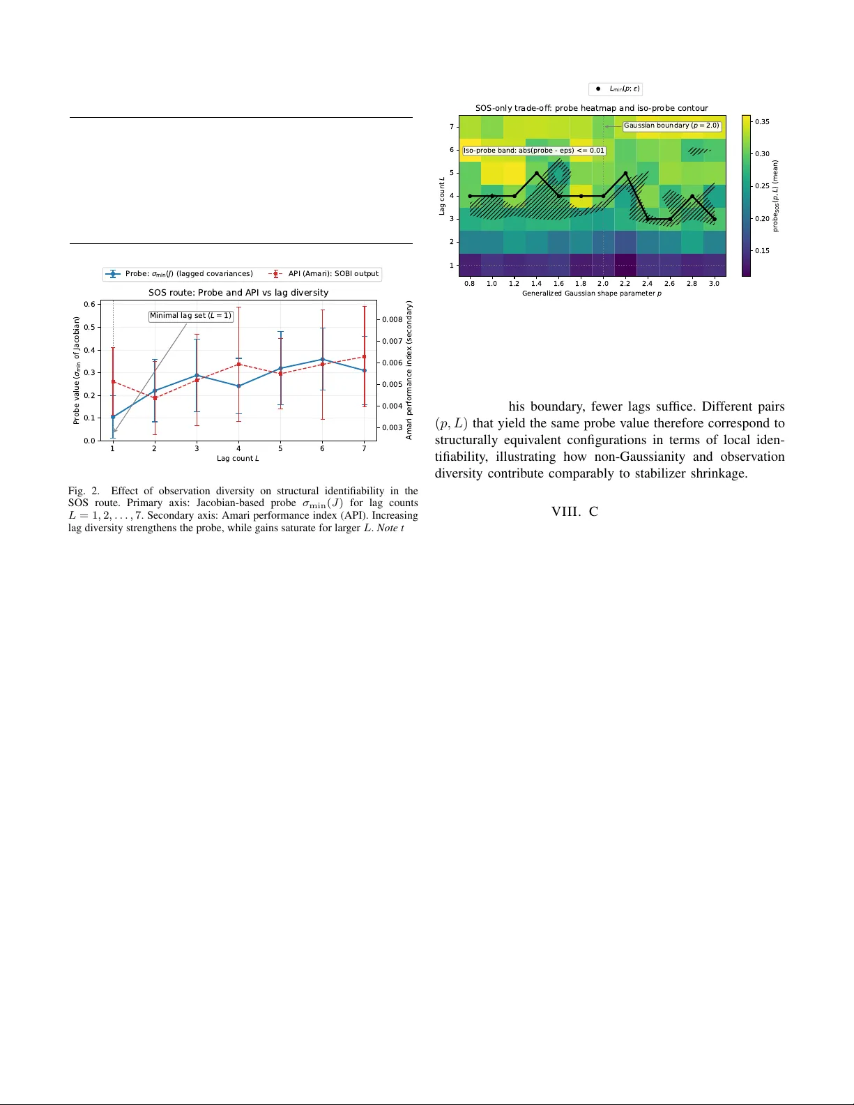
1 Identifiability in Blind Source Separation through Stabilizer Shrinkage: Unifying Non-Gaussianity and Observ ation Di v ersity T omomi Ogaw a and Hiroki Matsumoto Abstract —Identifiability is a central issue in blind sour ce separation (BSS), determining whether latent sources can be uniquely recov ered from observed mixtur es. Classical approaches address identifiability either by exploiting source non-Gaussianity via higher-order statistics (HOS) or by enriching the observation structure through temporal, spatial, or multi-channel diversity using second-order statistics (SOS), and these r outes ar e often regarded as fundamentally differ ent. In this paper , we re visit identifiability in BSS from a structural perspective, inter preting it as constraint-induced reduction of residual ambiguity in the mix- ing model. Within this framework, the observation mechanism is viewed broadly to include both input-side statistical constraints and output-side observation structures. HOS-based and SOS- based approaches are then unified as mechanisms of stabilizer shrinkage , in which observation-induced constraints r educe an initially continuous ambiguity to a finite r esidual one. T o connect this structural viewpoint with finite-sample regimes, we introduce a Jacobian-based sensitivity probe as a numerical diagnostic of local identifiability . Numerical experiments show that increasing non-Gaussianity or observation diversity suppr esses the same residual symmetry , re vealing a structural trade-off between source statistics and observation design. These r esults pr ovide a unified interpretation of classical BSS methods and clarify how observation constraints govern identifiability . Index T erms —Blind source separation, identifiability , stabi- lizer , higher-order statistics, second-order statistics, observation diversity . I . I N T RO D U C T I O N Blind source separation (BSS) aims to recover latent source signals from observed mixtures without prior kno wledge of the mixing process, and identifiability lies at the core of this task [1]. Even when separation algorithms con v erge and standard performance indices appear satisfactory , residual am- biguities may remain [2]. Such ambiguities reflect intrinsic limitations of the observation mechanism rather than algorith- mic failure. Clarifying when and why they can or cannot be eliminated is therefore essential for interpreting classical BSS methods and for guiding the design of new ones. Classical studies of identifiability in BSS hav e largely followed two complementary routes [3]–[6]. Higher-order statistics (HOS)–based methods exploit deviations from Gaus- sianity to impose distributional constraints that are not acces- sible through second-order analysis [7]. In contrast, second- order statistics (SOS)–based methods enrich the observation T omomi Ogawa is with the Graduate School of Science and Engineering, T okyo Denki University , Saitama, Japan (e-mail: to.ogawa@mail.dendai.ac.jp). Hiroki Matsumoto is with the Graduate School of Engineering, Mae- bashi Institute of T echnology , Gumma, Japan (e-mail: matsumoto@maebashi- it.ac.jp). structure via temporal, spatial, or multi-channel div ersity , thereby imposing multiple correlation-based constraints [2], [8]. Throughout this paper , we use the term multi-SOS to refer to second-order statistics constructed from multiple lags or blocks (e.g., delayed covariance matrices in SOBI-type methods), in contrast to single-lag second-order statistics. These two routes are commonly regarded as fundamentally different, resulting in distinct algorithmic families and de- sign heuristics. Consequently , identifiability has typically been discussed either from the standpoint of source statistics or from that of observation di versity , with limited conceptual integration between the two. Recent data-driven and deep learning–based approaches further complicate this landscape [9], [10]. Although such methods often achieve strong empirical performance, they do not directly address the structural question of identifiability: to what extent does the observation mechanism itself resolve ambiguity , independently of model capacity or training data? This question motiv ates a structural treatment of identifiability based on ho w observations constrain admissible transforma- tions of the mixing model [11]. From this perspectiv e, identifiability is not viewed as an al- gorithmic outcome but as a property of the observation mech- anism itself. Specifically , it depends on whether observation- induced constraints reduce an initially continuous ambiguity to a finite residual one. In the sequel, this idea is formalized by introducing an observation-induced equi valence relation in Section II, characterizing the associated stabilizer of admis- sible transformations in Section IV, and examining its local manifestation through Jacobian sensitivity in Section V. W ithin this framework, observ ation statistics are interpreted as in v ariance constraints on the mixing matrix, and residual ambiguities correspond to transformations that preserve all enforced statistics. Identifiability is therefore characterized by the extent to which these constraints restrict the admissible transformation group. In particular , HOS-based approaches impose constraints primarily on the input side through as- sumptions on source statistics such as non-Gaussianity and independence, whereas multi-SOS-based approaches impose constraints on the output side by enriching the observation structure through temporal, spatial, or multi-channel div ersity in second-order statistics. Both classes of methods can thus be interpreted as mechanisms that reduce residual ambiguity by shrinking the stabilizer of the mixing model. This structural reduction, termed stabilizer shrinkage and formalized in Sec- tion IV -C, provides a unified viewpoint in which distributional information and observation di versity act as alternati ve sources 2 of constraint richness for ambiguity reduction. An immediate implication of this vie wpoint is that obser- vation mechanisms producing identical stabilizer shrinkage necessarily yield identical local identifiability properties, re- gardless of whether the constraints arise from HOS or from multi-SOS statistics. Dif ferences between algorithms there- fore reflect how stabilizer-reducing constraints are instantiated rather than fundamentally distinct identifiability principles. T o connect this structural analysis to finite-sample regimes, we introduce a Jacobian-based sensiti vity probe as a numerical diagnostic of local identifiability . The probe is used strictly as a measurement tool, not as a new identifiability criterion, to assess ho w strongly observation constraints suppress weakly observable perturbation directions. Because the Jacobian cap- tures the first-order response of the observ ation map, its nullspace reflects residual stabilizer directions, enabling diag- nostic comparison of dif ferent constraint configurations even when global identifiability conditions are formally satisfied. Controlled numerical experiments illustrate that (i) HOS constraints strengthen identifiability as non-Gaussianity in- creases, (ii) multi-lag SOS constraints recov er identifiability through observation div ersity e ven under Gaussian sources, and (iii) the trade-of f between these mechanisms can be visualized within a common structural frame work. The main contributions of this paper are summarized as follows: • A structural interpretation of identifiability in BSS based on constraint-induced ambiguity reduction, independent of specific separation algorithms. • A unified framew ork of stabilizer shrinkage that relates HOS-based and SOS-based approaches and clarifies their complementary roles. • A Jacobian-based sensiti vity probe as a practical diagnos- tic tool for visualizing local identifiability under finite- sample conditions. • Numerical experiments illustrating ho w non-Gaussianity and observation di versity contribute to ambiguity reduc- tion within a common structural probe. The remainder of the paper is org anized as follows. Sec- tion II introduces the problem formulation and inherent am- biguities. Section III revie ws classical HOS-based and SOS- based approaches from a constraint-oriented perspective. Sec- tion IV dev elops the structural viewpoint on observation- induced constraints and symmetry . Section V formalizes local identifiability via Jacobian sensitivity . Section VI examines the relationship between non-Gaussianity and observation di ver - sity , and Section VII presents numerical experiments v alidating the proposed interpretation. Section VIII concludes the paper and discusses implications for the design and diagnosis of observation constraints in blind source separation. Appendix A provides the formal definition of the Jacobian-based probe, while Appendix B summarizes representative counterexam- ples in which observ ation-induced constraints fail to reduce ambiguity . I I . P RO B L E M F O R M U L AT I O N A N D N OTA T I O N A. Blind Source Separation Model W e begin by fixing the basic blind source separation (BSS) model and the associated equi valence class, which serve as the reference throughout the paper . W e consider the standard linear instantaneous BSS model [1], [12] x ( t ) = H s ( t ) , (1) where s ( t ) ∈ R n denotes statistically independent source signals and H ∈ R m × n is an unkno wn mixing matrix. The objectiv e of BSS is to recover the source signals, or an equiv alent representation thereof, solely from the observed mixtures x ( t ) , without prior knowledge of H . Throughout this paper , we focus on square or overdeter - mined mixtures ( m ≥ n ), and consider both real-v alued and complex-v alued formulations, as they naturally arise in appli- cations such as audio signal processing and communication systems [13]. No specific algorithmic structure is assumed at this stage; the analysis is intended to be independent of particular separation methods [7]. When second-order statistics are inv olved, we assume that the observations are whitened using the sample cov ariance [3], [4]. Here, for a zero-mean vector process v ( t ) , we define Co v ( v ) := E [ v ( t ) v ( t ) ⊤ ] (or E [ v ( t ) v ( t ) ∗ ] in the complex- valued case), where E [ · ] denotes statistical expectation, ( · ) ⊤ the transpose, and ( · ) ∗ the conjugate transpose. Under the linear model (1), the covariance of the observa- tions satisfies Co v ( x ) = H Co v( s ) H ⊤ . (2) In practice, whitening is achie ved by a linear transformation W such that Co v ( W x ) = I , (3) where I denotes the identity matrix of appropriate dimen- sion. Under (1), this implies that the effecti ve mixing matrix W H satisfies ( W H )( W H ) ⊤ = I in the real-v alued case (or ( W H )( W H ) ∗ = I in the complex-valued case), and can therefore be re garded as orthogonal (or unitary). In the following, we adopt the common con vention of absorbing the whitening transform into the observation, and reuse the symbol x to denote the whitened signal. Accordingly , without loss of generality , the mixing matrix can be considered up to a residual right-orthogonal (or uni- tary) transformation. Specifically , one may assume that after whitening, Co v ( x ) = I = ⇒ H ∼ H Q, (4) where the symbol ∼ denotes an equi valence relation on the set of mixing matrices, identifying representations that dif fer only by a residual right-orthogonal (or unitary) transformation. The residual transformation Q satisfies Q ∈ ( O ( n ) , real-valued case , U ( n ) , complex-v alued case , (5) reflecting the fact that whitening fixes the zero-lag cov ariance up to an orthogonal or unitary change of basis. Here, O ( n ) and 3 U ( n ) denote the orthogonal and unitary groups of dimension n , respectively , with dimensions consistent with the whitened model. The symbol I should not be confused with the index set I used later to label observ ation constraints. This preprocessing does not alter identifiability in the sense considered here. Rather, it isolates the residual ambiguities to orthogonal (or unitary) transformations, a property that plays a central role in the subsequent analysis. It is well known that, even under ideal conditions, the BSS problem does not admit a unique solution. Instead, recov ered sources are determined only up to inherent ambiguities. In particular , demixing solutions related by permutation and component-wise scaling (or phase rotations in the complex- valued case) are indistinguishable from the observ ations [3]. Accordingly , throughout this paper we regard two mixing matrices as equiv alent if H ∼ H P D , (6) where P is a permutation matrix and D is a nonsingular diagonal matrix (representing scaling or phase factors). This equiv alence relation fixes the notion of identifiability consid- ered in the sequel. B. Ambiguities and Equivalence up to Inher ent T ransforma- tions A fundamental characteristic of blind source separation is that its solutions are not unique, e ven in the absence of noise and estimation errors. This non-uniqueness does not arise from algorithmic imperfections, but is intrinsic to the BSS model itself [2], [14]. Specifically , certain transformations applied to the recov ered sources produce alternati ve solutions that remain consistent with the observed mixtures. In practice, the inherent ambiguities described by (6) include permutations of the source order and component-wise scaling, or phase rotations in the complex-v alued case. Such transfor- mations preserve the validity of the separation in the sense that they lead to reconstructed sources compatible with the observed data, despite dif ferences in parameter representation. Throughout this paper , equi valence is understood strictly in this BSS-specific sense. At this stage, no additional algebraic or group-theoretic structure is assumed; the purpose of this subsection is solely to clarify which ambiguities are considered inherent to the model. This perspecti ve is essential for interpreting identifiability in blind source separation. Rather than asking whether a unique parameter estimate e xists, the rele vant question is which ambiguities can or cannot be resolved by the av ailable information [15]. Identifiability is therefore determined by the extent to which observation-deri ved constraints restrict the equiv alence class (6) [2]. In the following subsection, this viewpoint is formalized by examining ho w different classes of observation statistics act as constraints that progressively limit the set of admissible transformations. C. Observation Statistics as Constraint-Inducing Information Throughout this paper , identifiability is considered up to the finite inherent ambiguities described in Section II-B (per- mutation and component-wise scaling, or phase rotations in the complex-v alued case). After whitening (Section II-A), these finite ambiguities are preceded by a continuous right- orthogonal (or unitary) freedom, reflecting the fact that second- order statistics alone cannot distinguish right-unitary reparam- eterizations of the mixing matrix. The general linear group GL( n ) is introduced here as a con venient parametrization of admissible reparameterizations of the mixing matrix before observation-induced constraints are imposed; after whitening, the rele vant residual transformations reduce locally to right- orthogonal (or unitary) actions as discussed in Section II-A. In blind source separation, the only information av ailable for resolving these ambiguities arises from statistical properties of the observed signals. W e therefore interpret observation statis- tics structurally , as constraints imposed by the observation mechanism itself, which restrict admissible transformations of the mixing matrix while remaining consistent with the observed data. T o formalize this viewpoint, we introduce an observation map Φ : H 7− →  A i ( H )  i ∈I , (7) where each A i ( H ) is a matrix-v alued quantity induced by a chosen class of observation statistics. The index set I speci- fies which statistical constraints are imposed simultaneously . T ypical examples include higher-order cumulant matrices in HOS-based approaches or cov ariance-based operators in SOS- based approaches [5], [16]. Each operator A i ( H ) is defined by applying a fixed, predetermined construction rule (e.g., a population cumulant or cov ariance operator) to the model x ( t ) = H s ( t ) ; the same construction rule is applied when ev aluating A i ( H G ) for any admissible transformation G . For example, in the HOS case A i ( H ) may correspond to pop- ulation fourth-order cumulant matrices, whereas in the SOS case it may represent lagged covariance operators e valuated at different lags. For clarity , the term multi–SOS is used to collectively refer to second-order constraint families inv olving multiple opera- tors, including but not limited to lagged cov ariance matrices, multi-sensor or multi-channel observations, block or oversam- pled cov ariance structures, and cov ariance operators obtained under multiple experimental conditions [5], [17], [18]. In this usage, specific instances such as multi-lag SOS correspond to concrete realizations based on temporal lag div ersity . In contrast, the labels HOS-based and SOS-based are used when emphasizing the type of statistics being exploited, whereas the term multi–SOS highlights the structural lev el at which multiple second-order operators jointly impose constraints. The collection { A i ( H ) } i ∈I represents in variants of the observation: an y admissible transformation of H must pre- serve all of these quantities. Specifically , a transformation G ∈ GL( n ) is said to be compatible with the observation if A i ( H G ) = A i ( H ) , ∀ i ∈ I . (8) This in v ariance condition can be equiv alently rewritten as A i ( H G ) = A i ( H ) ∀ i ⇐ ⇒ Φ( H G ) = Φ( H ) , (9) 4 which makes explicit that admissible transformations are those that lea ve the observation map unchanged. Accordingly , we define the residual ambiguity set induced by the observation map Φ as Stab( I ) ≜  G ∈ GL( n )   A i ( H G ) = A i ( H ) , ∀ i ∈ I  . (10) The terminology “stabilizer” is used here in the standard sense of group actions, referring to the subgroup of transfor- mations that leave a giv en object in variant (see, e.g., [19]). The set Stab( I ) captures the remaining symmetries of the mixing matrix that cannot be resolved from the av ailable statis- tics. In practice, dif ferent choices of observation statistics lead to different degr ees of stabilizer r eduction : while whitening alone leav es a continuous right-unitary stabilizer , appropriately chosen and sufficiently rich observ ation constraints can, under well-understood conditions, reduce this continuous ambiguity to a finite residual group. In this sense, identifiability is gov erned by how strongly the observation map Φ restricts admissible transformations of H , rather than by the numerical procedure used to estimate it. Remark on identifiability: Identifiability in blind source separation does not arise from output non-Gaussianity alone, nor from structural richness of the input process when such structure is not fixed by the observ ation operators. Instead, identifiability emerges only when source-side constraints (e.g., non-Gaussianity combined with independence) or output-side operator di versity effecti vely reduce the continuous right- unitary freedom to a finite residual ambiguity . Formal coun- terexamples illustrating these asymmetries are summarized in Appendix B. D. Scope and Assumptions The scope of this paper is deliberately restricted in order to focus on the structural aspects of identifiability in blind source separation. Specifically , we consider linear instantaneous mix- ture models with statistically independent sources [20], as introduced in Section II-A. This setting encompasses a broad class of classical BSS problems while allowing the ef fects of different observation constraints to be examined without confounding factors arising from model comple xity . The analysis primarily addresses separation methods based on second-order and higher-order observation statistics, in- cluding those e xploiting temporal, spatial, or multi-observ ation div ersity . No assumptions are made on a particular algorithmic implementation, and the discussion is not tied to specific optimization procedures. Instead, the emphasis is placed on how dif ferent classes of statistical information constrain the underlying model and influence the resolution of inherent ambiguities. Sev eral extensions of the basic BSS model are intentionally not considered [9], [10], [21]. These include nonlinear or con voluti ve mixtures, deep learning–based separation frame- works, and problem formulations that rely on supervised or semi-supervised training. While these settings are of practical interest, they introduce additional sources of ambiguity and inductiv e bias that obscure the structural ef fects studied here. By limiting attention to the classical linear BSS frame work, the analysis aims to isolate and clarify the role of observation- induced constraints in shaping identifiability . I I I . B A C K G RO U N D : H O S - B A S E D A N D S O S - B A S E D B L I N D S O U R C E S E PA R A T I O N Blind source separation has been studied extensi vely under a variety of assumptions and problem settings. Among classical approaches, methods based on higher-order statistics (HOS) and those based on second-order statistics (SOS) hav e played a central role and are often treated as distinct methodological families. This section briefly revie ws these two classes, focus- ing on their roles as constraint-inducing mec hanisms rather than on algorithmic details. A. HOS-Based Appr oaches HOS-based approaches exploit the non-Gaussianity of source signals by introducing constraints derived from higher- order moments or cumulants, which are in visible to second- order analysis [3], [4], [7], [16], [22]–[25]. From a structural viewpoint, HOS-based methods impose constraints of the form A i ( H G ) = A i ( H ) , i ∈ I HOS , (11) where A i ( H ) denotes a matrix induced by higher-order statis- tics (e.g., cumulant matrices), G ∈ GL( N ) represents an admissible transformation of the mixing matrix, and I HOS index es the chosen set of HOS constraints. Equation (11) expresses the fact that only transformations preserving higher- order statistical structure remain compatible with the observ a- tion. A key advantage of HOS-based methods is their ability to eliminate ambiguities that persist under purely second-order analysis, particularly when source distributions deviate suffi- ciently from Gaussianity . At the same time, the effecti veness of these constraints depends on the reliability of higher -order statistical estimation, which can be sensiti ve to finite-sample effects and noise. B. SOS-Based Appr oaches In contrast, SOS-based approaches rely on structural di- versity in the observations, without assuming specific source distributions [2], [5], [6], [8], [17], [18], [26]. By exploiting multiple time lags, sensor arrays, or observation blocks, they introduce collections of second-order constraints. A typical SOS formulation considers a collection of cov ari- ance matrices R z ( τ ) = E  z ( t ) z ( t − τ ) ⊤  , τ ∈ I SOS , (12) where z ( t ) denotes the observed (often whitened) signal, and I SOS specifies a set of nonzero lags or observ ation conditions. Each lag τ induces a second-order constraint, and separation is achie ved by enforcing joint compatibility across all selected lags. Structurally , SOS-based methods restrict admissible trans- formations by requiring simultaneous consistency with multi- ple second-order relations. While any single covariance con- straint may leav e substantial ambiguity , their combination can 5 significantly reduce the set of transformations that preserve all imposed correlations. Such methods are often viewed as statistically robust and computationally ef ficient, especially in scenarios where non-Gaussianity is weak or unreliable but sufficient observation div ersity is av ailable. C. Structural Comparison Although HOS-based and SOS-based methods are often presented as alternative strategies, both act by introducing additional in variance constraints that restrict admissible trans- formations of the mixing model. The distinction lies in the sour ce of constraint information: distrib utional properties in the HOS case and observation div ersity in the SOS case. From the unified viewpoint dev eloped in Section II-C, both families can be interpreted as imposing collections of in vari- ance constraints of the form (11) or (12), which progressively restrict the set of admissible transformations compatible with the observed data. Identifiability is therefore governed by how strongly these constraints reduce the stabilizer, rather than by the statistical order or algorithmic realization. Counterexamples in which indi vidual constraint families f ail to reduce the stabilizer are summarized in Appendix B. I V . S T R U CT U R A L V I E W P O I N T : O B S E RV AT I O N C O N S T R A I N T S A N D S Y M M E T RY A. Observation-Induced Constraints on the Mixing Model The statistical information e xtracted from observed mixtures imposes structural constraints on the admissible transforma- tions of the mixing model: only those transformations that preserve the observed statistics remain compatible with the data, while others lead to inconsistencies. Here, Φ( H ) = { A i ( H ) } i ∈I refers to the observation map introduced in Section II-C. As defined in (10), the set of transformations that leav e all constraint objects in variant forms the stabilizer Stab( I ) [19]. This stabilizer represents the residual ambiguity of the mixing model under the imposed observation constraints. When only a single class of observation statistics is en- forced, the corresponding index set I is typically limited, and the stabilizer Stab( I ) remains nontrivial. Such constraints eliminate only those transformations that violate the specific statistical properties being enforced, leaving a family of ad- missible transformations that reflect intrinsic ambiguities of the separation model. Crucially , the stabilizer Stab( I ) is a global object: it characterizes residual ambiguities at the level of exact in vari- ance under the observation map. While this global charac- terization is conceptually clear , it does not directly indicate how ambiguity reduction manifests under finite samples or small perturbations. This observation motiv ates the need for a complementary local characterization of stabilizer reduction, which is dev eloped in the subsequent sections via Jacobian- based sensiti vity analysis. B. Residual Ambiguities under Multiple Constr aints Even when observation statistics impose nontrivial con- straints on the mixing model, residual ambiguities generally remain if only a single class of constraints is enforced. Such ambiguities correspond to nontrivial elements of the stabilizer Stab( I ) associated with the chosen observ ation operators, and cannot be ruled out based on that information alone. These residual symmetries are not accidental; rather , they reflect intrinsic structural properties of the separation model under limited observ ational constraints. When multiple classes of observation statistics are consid- ered simultaneously , each class imposes a distinct inv ariance on the mixing model and therefore induces its own stabi- lizer . Let I 1 and I 2 denote index sets associated with two different families of observation operators. A transformation is compatible with both constraints if and only if it preserves both in v ariances. Accordingly , the admissible transformations under multiple constraints are characterized by the following elementary b ut structurally important relation. Lemma 1 (Intersection of stabilizers under multiple con- straints): Let I 1 and I 2 be inde x sets corresponding to tw o different families of observation operators. Then the stabilizer associated with their joint constraint satisfies Stab( I 1 ∪ I 2 ) = Stab( I 1 ) ∩ Stab( I 2 ) . (13) Pr oof: By definition of the stabilizer gi ven in (10), a trans- formation belongs to Stab( I ) if and only if it preserves every observation operator index ed by I . Applying this definition to the union I 1 ∪ I 2 , a transformation belongs to Stab( I 1 ∪ I 2 ) precisely when it preserves all operators in both families. This condition is equiv alent to requiring membership in both Stab( I 1 ) and Stab( I 2 ) , which establishes (13). The key point is that the benefit of combining multiple constraints does not depend on their specific algorithmic realization, b ut on how their induced stabilizers intersect at a structural lev el. Constraints derived from dif ferent sources of statistical information tend to eliminate complementary classes of symmetries, even when each constraint alone is insufficient for identifiability . At the same time, the intersection relation in Lemma 1 remains a global statement. It specifies which transformations are ultimately excluded, but not how such exclusion manifests under finite perturbations or finite data. This observ ation motiv ates the introduction of a local perspectiv e that can quantify stabilizer reduction in practice. C. Accumulation of Constraints and Structural Ambiguity Reduction When multiple observation-induced constraints are enforced simultaneously , their effects accumulate through successi ve restrictions of the stabilizer . As additional constraint families are incorporated, the index set I gro ws, and the stabilizer Stab( I ) defined in (10) is progressively reduced through repeated intersections of the form (13). W e refer to this pro- gressiv e reduction of admissible transformations as stabilizer shrinkage . 6 From a global standpoint, stabilizer shrinkage reflects a systematic simplification of the symmetry inherent in the mixing model under limited observation. Each ne wly imposed class of observ ation statistics excludes transformations that were pre viously admissible, thereby reducing the de grees of freedom associated with residual ambiguity . This reduction is induced by the observation mechanism itself and should not be confused with numerical re gularization or estimator -dependent effects. In practical settings, different observation statistics restrict different subsets of the original continuous right-unitary free- dom. As a consequence, distinct constraint families may lead to comparable ambiguity reductions ev en when their statistical origins differ . This explains why HOS-based and multi-SOS- based approaches, despite relying on different forms of statis- tical information, can exhibit structurally similar identifiability behavior . T o connect this global notion of ambiguity reduction to a local and tractable description, we explicitly exploit the fact that GL( n ) is a Lie group and that Stab( I ) forms a closed Lie subgroup, whose local structure is characterized by its associated Lie algebra (cf., e.g., [27]). As observ ation constraints accumulate, stabilizer shrinkage manifests not only as a set-theoretic reduction of admissible transformations, but also as a reduction in the dimension of the tangent space at the identity . From a dimensional perspective, this progressiv e reduction can be schematically expressed as dim T I Stab( I ) ↓ as constraints accumulate . (14) This local reduction provides a direct measure of how strongly the observation statistics restrict infinitesimal right-unitary perturbations of the mixing matrix. The tangent-space viewpoint naturally bridges global sym- metry reduction and local sensitivity analysis. In particular , it moti vates a Jacobian-based characterization of local iden- tifiability , in which the sensitivity of the observation map to infinitesimal reparameterizations determines whether residual ambiguities persist locally . This perspecti ve forms the basis of the Jacobian analysis dev eloped in Section V. Overall, this structural viewpoint clarifies when and how identifiability improves as additional observation statistics are incorporated. By framing ambiguity reduction in terms of stabilizer shrinkage and its manifestation in the tangent space, this section provides a coherent transition from global ambiguity analysis to the local identifiability results presented next. V . L O C A L I D E N T I FI A B I L I T Y V I A J A C O B I A N S E N S I T I V I T Y A. Local P erturbations and Constraint Sensitivity Identifiability in blind source separation is often discussed as a global or asymptotic property . In practical settings with finite samples and imperfect statistical estimates, howe ver , identifiability manifests through the local beha vior of the model. It is therefore informative to examine ho w small per- turbations of the mixing model af fect the observ ation statistics enforced by a giv en set of constraints. Let Stab( I ) denote the stabilizer associated with a set of observation constraints, as defined in Section IV. Since GL( n ) is a Lie group, admissible transformations in a neighborhood of the identity can be expressed through infinitesimal perturba- tions. After whitening, these reduce locally to right-orthogonal directions, moti vating the use of ske w-symmetric generators. Specifically , we consider local perturbations of the form H ( ε ) = H exp( ε Ω) , Ω ⊤ = − Ω , (15) where ε ∈ R is a small scalar parameter and Ω is a ske w-symmetric matrix generating a local right action. This parameterization preserv es orthogonality after whitening and provides a natural coordinate system for local analysis. Under such perturbations, some directions Ω induce no- ticeable changes in the observation statistics, while others leav e them nearly unchanged. The former correspond to direc- tions strongly constrained by the imposed statistics, whereas the latter indicate residual ambiguities that remain weakly constrained. Sensiti vity to local perturbations therefore pro- vides a natural lens through which the practical strength of observation-induced constraints can be assessed. B. Jacobian as a Numerical Pr obe of Residual Ambiguity The local sensitivity of observ ation-induced constraints to infinitesimal perturbations can be examined through the Jaco- bian of the observ ation map Φ defined in (7). The Jacobian with respect to the local perturbation (15) is defined as J ( H ) = ∂ ∂ ε Φ( H exp( ε Ω))     ε =0 . (16) This Jacobian captures the first-order response of the obser- vation constraints to infinitesimal transformations generated by Ω . Locally , stabilizer shrinkage corresponds to a reduction of admissible tangent directions, and the Jacobian therefore indicates which perturbation directions remain compatible with the imposed constraints. In practice, the Jacobian is used as a numerical probe of local constraint strength. Small Jacobian responses correspond to transformations that leav e the statistics nearly in variant, in- dicating weakly constrained directions associated with residual ambiguities. Con versely , large responses indicate directions strongly restricted by the observation constraints. For completeness, the formal definition of the Jacobian- based probe and its local parameterization are summarized in Appendix A. C. Relation to Structural Ambiguity Reduction The numerical behavior revealed by Jacobian sensitivity corresponds directly to the structural ambiguity reduction dis- cussed in Section IV. Observation-induced constraints restrict admissible transformations at the group lev el through stabilizer shrinkage, and this restriction appears locally through the behavior of the Jacobian. Perturbation directions that remain weakly constrained by the imposed statistics correspond to tangent directions of the stabilizer Stab( I ) at the identity . Here, T I Stab( I ) denotes the tangent space of the stabilizer Stab( I ) at the identity element, 7 representing the space of infinitesimal admissible transfor- mations. Such relationships between infinitesimal in variances and the tangent space of a symmetry group are standard in Lie theory (cf., e.g., [27]). When Stab( I ) forms a regular Lie subgroup of GL( n ) , its tangent space at the identity is naturally identified with the Lie algebra associated with the stabilizer , as e xpressed in (18). At the lev el of first-order sensitivity , this relation can be summarized by k er J ( H ) ⊆ T I Stab( I ) , (17) indicating that locally unobservable perturbations align with infinitesimal stabilizer directions. Under the same regularity conditions, this inclusion tightens to k er J ( H ) = T I Stab( I ) . As additional constraints are accumulated, the stabilizer shrinks and its local tangent space decreases accordingly . Numerically , this reduction manifests as suppression of weakly sensitiv e directions in the Jacobian, reflected by the collapse of k er J ( H ) and the gro wth of its smallest singular value. V I . U N I F Y I N G N O N - G AU S S I A N I T Y A N D O B S E RV A T I O N D I V E R S I T Y A. Motivation Classical blind source separation methods based on higher- order statistics (HOS) and those based on second-order statis- tics (SOS) are often treated as fundamentally different. How- ev er , from the structural viewpoint dev eloped in Sections IV– V, both classes of methods reduce the same object: the residual ambiguity captured by the stabilizer of the observation constraints. Let I denote the index set of constraint operators associated with a given observation mechanism, and recall the definition of the stabilizer Stab( I ) gi ven in (10). Identifiability improv es as this stabilizer shrinks under increasingly rich constraint families, regardless of how the constraints are instantiated. From this perspectiv e, the apparent dichotomy between HOS-based and SOS-based methods reflects dif ferent choices of the constraint index set I rather than fundamentally distinct identifiability mechanisms. HOS-based methods correspond to constraint families I HOS induced by higher-order statistics, whereas SOS-based methods correspond to constraint families I SOS induced by observation di versity . A unified treatment therefore requires comparing ho w these dif ferent inde x sets reduce the same stabilizer , rather than comparing algorithms in isolation. B. Numerical Identifiability via Local Sensitivity While the stabilizer Stab( I ) provides a global charac- terization of residual ambiguity , its direct computation or comparison is generally intractable. As discussed in Section V, a local characterization is obtained by examining the Jacobian of the observation map. Let J ( H ) denote the Jacobian defined in (16). The kernel k er J ( H ) characterizes infinitesimal perturbations that remain compatible with the imposed constraints and therefore pro- vides a local representation of stabilizer shrinkage. In partic- ular , under suitable regularity conditions, k er J ( H ) ∼ = lie (Stab( I )) , (18) which links global symmetry reduction to local sensitivity . Here, lie (Stab( I )) denotes the Lie algebra associated with the stabilizer , that is, the space of infinitesimal generators of trans- formations that preserve the imposed observation constraints. In practice, rather than using k er J ( H ) as a binary identifia- bility criterion, we summarize local constraint strength through the smallest singular v alue σ min ( J ( H )) , which measures how strongly stabilizer directions are suppressed. This quantity serves as a numerical probe of stabilizer shrinkage rather than as an estimator or optimality metric. C. Instantiating Stabilizer Shrinkage with HOS and SOS The unifying interpretation becomes explicit when HOS- based and SOS-based constraints are examined within the same stabilizer framew ork. For HOS-based methods, the con- straint family I HOS is determined by higher -order cumulant operators, whereas for SOS-based methods, the constraint family I SOS is determined by collections of second-order cov ariance operators. Although I HOS and I SOS differ in their statistical origins, both act on the same object through stabilizer intersection: Stab( I HOS ∪ I SOS ) = Stab( I HOS ) ∩ Stab( I SOS ) , (19) as established in (13). Consequently , identifiability improv e- ments obtained by increasing non-Gaussianity or observation div ersity correspond to different ways of shrinking the same stabilizer . This formulation clarifies why non-Gaussianity and obser- vation di versity can be viewed as alternative sources of con- straint richness. Different constraint families reduce the same stabilizer through dif ferent mechanisms, while their effect on local identifiability is captured by the same Jacobian-based sensitivity . From a systems perspectiv e, architectural choices (e.g., the number of lags or sensing di versity) and statistical assumptions influence identifiability only through the e xtent to which they reduce the dimension of the stabilizer , providing a structural guideline for the design of observation mechanisms in blind source separation. V I I . N U M E R I C A L E X P E R I M E N T S Throughout this section, we use the Jacobian-based probe σ min ( J ) as a diagnostic tool to visualize structural ambiguity r eduction under dif ferent observ ation constraints. The absolute scale of the probe depends on the specific constraint family and is not intended for cross-experiment comparison or for ranking HOS- and SOS-based approaches. All experiments are designed to validate structural predictions derived from stabilizer shrinkage, rather than to benchmark separation al- gorithms. 8 A. Experimental Setup and Evaluation Measur es W e ev aluate the structural effects discussed in Sections IV– V using controlled numerical experiments. The purpose of this section is not algorithm benchmarking or performance comparison, but to visualize ho w ambiguity reduction emerges through the accumulation of observation-induced constraints. a) Model and pr epr ocessing.: W e consider a real-valued, linear instantaneous BSS model y = H s with an equal number of sources and observations ( n = m ). Unless otherwise stated, we set n = m = 3 and whiten all mixtures using the sample cov ariance. After whitening, we select a reference mixing matrix H 0 = I as a canonical representativ e of the equiv alence class discussed in Section II-A, and ev aluate identifiability locally around this reference point. Accordingly , the remaining ambiguity corresponds to right-orthogonal transformations. b) Primary pr obe.: Let Φ( H ) denote the collection of observation statistics introduced in Section II-C, e valuated under a given experimental configuration. Local sensitivity is probed using the right-orthogonal perturbation parameter- ization introduced in Section V -A (cf. (15)), together with the Jacobian defined in Section V -B (cf. (16)). In the present experiments, the Jacobian is ev aluated at the reference point H 0 = I , and local sensitivity is assessed via infinitesimal perturbations around this point. Our scalar diagnostic is defined as prob e( H 0 ) := σ min  J ( H 0 )  , (20) which summarizes how strongly residual stabilizer directions are suppressed locally . All quantities are estimated from finite samples; we report Monte Carlo means and dispersion of prob e( H 0 ) . c) Secondary index (sanity check only).: As a secondary reference, we optionally report the Amari performance index (API) as a sanity check [22]. The API is not used to select algorithms or tune parameters; structural effects are assessed solely through the probe. d) Implementation.: All experiments were implemented in Python using standard numerical libraries (NumPy/SciPy) and executed in a CPU-based environment. No GPU-specific operations or platform-dependent optimizations were used. B. Effect of Higher -Order Statistics (HOS) T able I summarizes the simulation settings for the HOS- based experiments, including the choice of the reference mix- ing matrix H 0 used for local sensitivity ev aluation. These set- tings are chosen to isolate the effect of source non-Gaussianity on structural identifiability under higher-order constraints. Sources are i.i.d. generalized Gaussian, where the shape parameter p controls de viation from Gaussianity , with the Gaussian boundary at p = 2 . 0 . Higher-order information is incorporated through symmetric matrices deriv ed from fourth- order cumulants, constructed using the standard J ADE proce- dure. The resulting behavior of the Jacobian-based probe ev alu- ated at H 0 is shown in Fig. 1. As predicted by the structural analysis, the probe collapses near the Gaussian boundary ( p = 2 . 0 ), consistent with the vanishing of fourth-order T ABLE I S I MU L A T I O N S E T T IN G S F O R T H E H O S E X P E RI M E N T . Number of sources/observations n = m 3 Sample length T 1 × 10 5 Monte Carlo trials 50 Whitening Y es Reference mixing matrix H 0 = I Source distrib ution Generalized Gaussian Shape parameters p { 0 . 8 , 1 . 0 , 1 . 5 , 2 . 0 , 3 . 0 } HOS constraints Fourth-order cumulant matrices 1.0 1.5 2.0 2.5 3.0 Generalized Gaussian shape parameter p 0 1 2 3 4 5 6 7 8 P r o b e v a l u e ( m i n o f J a c o b i a n ) ( p r i m a r y ) Gaussian (p=2.0) HOS r oute: P r obe and API vs non- Gaussianity 0.0 0.1 0.2 0.3 0.4 0.5 0.6 Amari inde x (secondary) P r o b e : m i n ( J ) [ J A D E ] API (Amari) Fig. 1. Effect of source non-Gaussianity on structural identifiability in the HOS route. Primary axis: Jacobian-based probe σ min ( J ) computed from fourth-order cumulant constraints. The probe collapses near the Gaussian boundary ( p = 2 . 0 ) and increases for non-Gaussian sources. Secondary axis: Amari performance index (API). Error bars indicate Monte Carlo dispersion. Note that the absolute scales of both the primary probe and the secondary separation index are experiment-dependent and should not be compar ed acr oss differ ent figur es or constraint families. cumulants and the persistence of stabilizer directions under Gaussian sources. As p departs from 2 . 0 , the probe increases, reflecting progressiv e acti vation of higher-order constraints and corresponding stabilizer shrinkage. The API is sho wn only as a sanity check and confirms degradation of separation quality in the Gaussian case. C. Effect of Observation Diversity via Multi-Lag SOS W e next examine ambiguity reduction dri ven by observation div ersity using multi-lag second-order statistics, without rely- ing on higher -order information. The corresponding simulation settings are summarized in T able II. Sources are Gaussian AR(1) processes s i ( t ) = a i s i ( t − 1) + u i ( t ) , u i ( t ) ∼ N (0 , 1) , with distinct coefficients ( a 1 , a 2 , a 3 ) = (0 . 2 , 0 . 6 , 0 . 9) . Lagged cov ariance matrices of the whitened observations, R z ( τ ) = E [ z ( t ) z ( t − τ ) ⊤ ] , τ ∈ T L , constitute the SOS constraints. Figure 2 reports the resulting probe values ev aluated at the reference mixing matrix H 0 as a function of the number of lags L . For the minimal lag set ( L = 1 ), the probe remains small, indicating weak constraint strength. As additional lags are included ( L > 1 ), the probe increases overall, reflect- ing progressi ve suppression of residual stabilizer directions 9 T ABLE II S I MU L A T I O N S E T T IN G S F O R T H E S O S E X P E RI M E N T . Number of sources/observations n = m 3 Sample length T 1 × 10 5 Monte Carlo trials 50 Whitening Y es Reference mixing matrix H 0 = I Source model Gaussian AR(1) AR coef ficients ( a 1 , a 2 , a 3 ) (0 . 2 , 0 . 6 , 0 . 9) Lag set T L { 1 , 2 , . . . , L } Lag count L { 1 , 2 , 3 , 4 , 5 , 6 , 7 } SOS constraints Lagged cov ariance matrices 1 2 3 4 5 6 7 L a g c o u n t L 0.0 0.1 0.2 0.3 0.4 0.5 0.6 P r o b e v a l u e ( m i n o f J a c o b i a n ) M i n i m a l l a g s e t ( L = 1 ) SOS r oute: P r obe and API vs lag diversity 0.003 0.004 0.005 0.006 0.007 0.008 Amari perfor mance inde x (secondary) P r o b e : m i n ( J ) ( l a g g e d c o v a r i a n c e s ) API (Amari): SOBI output Fig. 2. Effect of observation div ersity on structural identifiability in the SOS route. Primary axis: Jacobian-based probe σ min ( J ) for lag counts L = 1 , 2 , . . . , 7 . Secondary axis: Amari performance index (API). Increasing lag diversity strengthens the probe, while gains saturate for larger L . Note that the absolute scales of both the primary pr obe and the secondary separation index are experiment-dependent and should not be compar ed across differ ent figur es or constraint families. through accumulated temporal constraints. For larger L , gains diminish due to finite-sample effects. The API remains nearly constant, indicating that separation quality is already saturated, while structural ambiguity continues to shrink. D. T rade-off Between Sour ce Statistics and Observation Di- versity Finally , we visualize the trade-of f between source statistics and observation div ersity using second-order observation con- straints, without explicitly combining higher-order statistics. Here, the shape parameter p characterizes the source pro- cess only and does not enter the SOS constraint operators themselves; the probe prob e SOS is computed exclusi vely from second-order (lagged cov ariance) operators, while v arying p modifies the effecti ve second-order structure av ailable after whitening. For each ( p, L ) , we e valuate the Jacobian-based probe defined in (20) for the SOS constraint family: prob e SOS ( p, L ) := σ min  J SOS ( H 0 )  . (21) Based on this quantity , we define the minimal lag count required to reach a target sensitivity level ε as L min ( p ; ε ) := min { L : prob e SOS ( p, L ) ≥ ε } . (22) The resulting trade-off is summarized in Fig. 3. Near the Gaussian boundary , where statistical structure is weak, larger lag diversity is required to reach the same probe le vel. 0.8 1.0 1.2 1.4 1.6 1.8 2.0 2.2 2.4 2.6 2.8 3.0 G e n e r a l i z e d G a u s s i a n s h a p e p a r a m e t e r p 1 2 3 4 5 6 7 L a g c o u n t L Iso -pr obe band: abs(pr obe - eps) <= 0.01 G a u s s i a n b o u n d a r y ( p = 2 . 0 ) SOS- only trade- off : pr obe heatmap and iso -pr obe contour 0.15 0.20 0.25 0.30 0.35 p r o b e S O S ( p , L ) ( m e a n ) L m i n ( p ; ) Fig. 3. T rade-off between source statistics and observation diversity under second-order observation constraints. Heatmap: probe SOS ( p, L ) . Markers: L min ( p ; ε ) defined in (22). This visualization highlights structurally equiv a- lent configurations rather than performance optima. A way from this boundary , fe wer lags suf fice. Dif ferent pairs ( p, L ) that yield the same probe v alue therefore correspond to structurally equi valent configurations in terms of local iden- tifiability , illustrating ho w non-Gaussianity and observation div ersity contribute comparably to stabilizer shrinkage. V I I I . C O N C L U S I O N This paper examined identifiability in blind source sepa- ration (BSS) from a structural standpoint, focusing on how observation-induced constraints eliminate symmetry-induced ambiguities. HOS-based and SOS-based approaches were characterized as mechanisms that restrict the class of trans- formations consistent with the observ ed data. W ithin this formulation, identifiability is governed by the extent to which statistical constraints shrink residual ambiguities, and the classical distinction between HOS and SOS is attributed to the origin of the imposed constraints. T o connect this structural characterization with finite-sample behavior , we introduced a Jacobian-based sensitivity probe as a numerical diagnostic of local identifiability . Numerical experiments confirmed the structural interpretation: in the HOS route, the probe collapses near the Gaussian limit and increases with stronger non-Gaussian constraints; in the SOS route, increasing lag di versity strengthens the probe e ven under Gaussian sources; and their trade-off can be visualized within a common structural scale. These results provide a local characterization of residual ambiguities through the kernel and sensitivity of the Jacobian. Beyond individual mechanisms, the main contribution of this work is a constraint-centered reorganization of identi- fiability . By separating structural effects from algorithmic implementations, the proposed vie w clarifies why methods with different formulations often exhibit similar empirical be- havior and why additional constraints can improv e robustness ev en when con v entional performance indices saturate. From a circuits-and-systems perspecti ve, observation architecture choices (e.g., lag div ersity) and statistical assumptions influ- ence identifiability through their effect on stabilizer reduction 10 under finite-sample and computational constraints. In this sense, identifiability can be viewed as the collapse of an infinite equiv alence class to a finite residual ambiguity under observation-induced constraints (cf. Sections II-C and IV -C). Sev eral extensions naturally follow . The same structural analysis applies to complex-v alued formulations and to broader observation models, including conv olutiv e and block or oversampled settings, as well as to multi-way representa- tions arising in tensor -based formulations [28]. The Jacobian- based probe also supports a design-oriented e valuation of constraint configurations based on their ambiguity-suppressing effect. More generally , the proposed interpretation provides a basis for extending constraint-induced ambiguity reduction to other blind inference problems beyond classical BSS. Overall, by organizing identifiability around constraint- induced ambiguity reduction, this work clarifies the operating principles of classical BSS methods and provides a concise structural basis for the design and e valuation of future blind separation approaches. A P P E N D I X A F O R M A L D E FI N I T I O N O F T H E J A C O B I A N - B A S E D P R O B E A. Observation Relations and P arameterization This appendix formalizes the Jacobian-based probe used in Sections V and VII. All models, assumptions, and notation are identical to those introduced in Section II, and the local per- turbation model follows Section V. The purpose here is purely notational: to state the probe definition used in the numerical ev aluations, without introducing additional theoretical claims. Let Φ( H ) denote the observ ation map defined in (7), whose components depend on the chosen constraint family (e.g., HOS or multi–SOS). Throughout, local sensitivity is e valuated under right-orthogonal reparameterizations as in (15). B. Jacobian of Observation Relations Consider the local perturbation H ( θ ) = H exp( θ Ω) with Ω ⊤ = − Ω as in (15). The Jacobian of the observation map along this perturbation is defined by J ( H ) = ∂ ∂ θ Φ( H exp( θ Ω))     θ =0 , (23) which coincides with the definition used in (16). The Jaco- bian pro vides a first-order linearization of ho w the enforced observation statistics respond to infinitesimal right-orthogonal perturbations. It is emphasized that J ( H ) is used only as a local sensitivity probe. It is not associated with an estimator , likelihood func- tion, or statistical optimality criterion, and is introduced solely to quantify how strongly the imposed observation constraints respond to parameter perturbations. Concr ete instantiations of Φ( H ) .: The abstract observa- tion map Φ( H ) specializes to concrete forms depending on the constraint family . For HOS-based constraints, Φ HOS ( H ) =  C (4) k ( H )  K k =1 , (24) where C (4) k ( H ) denote symmetric matrices constructed from fourth-order cumulants (e.g., as in the J ADE construction). For SOS-based constraints with lag set T L = { 1 , . . . , L } , Φ SOS ( H ) =  R z ( τ ) | τ ∈ T L  , R z ( τ ) = E [ z ( t ) z ( t − τ ) ⊤ ] . (25) In both cases, we write Φ( H ) = { A i ( H ) } i ∈I where A i ( H ) denotes the i -th matrix-valued component of the observation map (e.g., A i ( H ) = C (4) k ( H ) for HOS-based constraints or A i ( H ) = R z ( τ ) for SOS-based constraints). For local sensi- tivity analysis, we use the stacked vector representation ϕ ( H ) obtained by vectorizing and concatenating these components: ϕ ( H ) =    v ec A 1 ( H ) . . . v ec A |I | ( H )    ∈ R |I | n 2 , (26) where vec( · ) denotes the standard column-wise vectorization of a matrix. The Jacobian J ( H ) ∈ R ( |I | n 2 ) × d with d = n ( n − 1) / 2 is then obtained by collecting directional deriv ativ es of ϕ ( H ) with respect to infinitesimal right-orthogonal pertur- bations of H , parameterized by a basis of ske w-symmetric generators Ω . C. Definition and Interpr etation of the Pr obe The Jacobian-based probe is defined as prob e( H ) := σ min ( J ( H )) , (27) where σ min ( · ) denotes the smallest singular value. Small values of probe( H ) indicate the presence of perturbation directions that leave the enforced statistics nearly unchanged, whereas lar ger values indicate stronger suppression of such weakly observable directions. This interpretation is consistent with the structural viewpoint in Section IV and the local analysis in Section V. Importantly , the probe does not define identifiability in a strict sense, nor does it characterize the full symmetry structure of the model. It is used in Section VII only as a diagnostic tool to visualize and compare the ef fects of different constraint configurations, without introducing ne w identifiability criteria. D. Practical Computation fr om Sample Statistics In experiments, the statistics entering Φ( H ) are estimated from finite data samples. Accordingly , J ( H ) and probe( H ) are computed using sample-based estimates, and the reported values reflect both the imposed structural constraints and estimation variability . All numerical results in Section VII are therefore av eraged over Monte Carlo trials and accompanied by dispersion measures. A P P E N D I X B S I T UAT I ON S I N W H I C H I D E N T I FI A B I L I T Y C O N S T R A I N T S D O N O T S H R I N K T H E S TA B I L I Z E R This appendix provides explicit examples that support the asymmetry stated in Section II-C (Remark on identifiability): “richness” alone does not shrink the stabilizer unless con- straints act at the appropriate lev el. All notation and assump- tions follo w Section II and Section II-C, and we focus only on the transformations that preserve the available observations. 11 A. Output Non-Gaussianity Alone Is Insuf ficient Assume that only the output distribution P y is observ ed, while no constraint is imposed on the source distribution P s . Then the right-unitary reparameterization H 7→ H U, U ∈ U ( n ) , (28) cannot be excluded from P y alone. Indeed, defining s ′ = U ∗ s yields the equiv alent factorization y = H s = ( H U ) s ′ , (29) so the same P y is compatible with an entire right-unitary orbit of mixing matrices. Hence, output non-Gaussianity by itself does not restrict the stabilizer of the mixing model. B. Input-Side Structural Diversity W ithout Source Constraints Is Also Insufficient Assume that the source process is Gaussian b ut e xhibits rich second-order structure (e.g., nontrivial multi-lag covariances, ov ersampled/block covariances, or cyclostationary second- order statistics). W ithout additional source-side constraints that fix a preferred representation, the same right-unitary reparameterization persists: s ′ ( t ) = U ∗ s ( t ) , H ′ = H U, U ∈ U ( n ) . (30) Gaussianity is preserved under unitary transformations, and second-order structure transforms by unitary congruence; for example, Σ s ′ ( τ ) := E [ s ′ ( t ) s ∗ ( t − τ )] = U ∗ Σ s ( τ ) U. (31) Thus, input-side second-order “richness” alone does not shrink the stabilizer unless additional constraints anchor the source representation. C. F ailur e of Single-La g SOS This subsection presents a minimal counterexample that isolates the limitation of a single output-side second-order constraint and clarifies why observation div ersity is essential for stabilizer shrinkage. All notation and assumptions follow Sections II–II-C, and we focus exclusi vely on the effect of lagged cov ariance operators. Accordingly , when only the single-lag cov ariance operator is enforced, the stabilizer remains the full unitary group, Stab( H ; Cov(0)) = U ( n ) , (32) and the corresponding Jacobian kernel is nontrivial, k er J ( H )  = { 0 } , (33) where J ( H ) denotes the Jacobian of the observation map defined in (16). This demonstrates that a single second-order constraint does not reduce the continuous right-unitary ambi- guity: infinitesimal right-unitary perturbations remain locally in visible to the enforced statistics. Now consider the addition of a second lag τ  = 0 , yielding the pair of operators { Σ y (0) , Σ y ( τ ) } . Under generic conditions—specifically , when the joint spectrum of the asso- ciated source cov ariance operators is simple—the joint com- mutant of these operators is finite. In this case, the stabilizer collapses to a finite set, and the local ambiguity v anishes: k er J ( H ) = { 0 } . (34) Thus, the inclusion of a second lag is sufficient to eliminate the continuous right-unitary freedom that persists under a single- lag constraint. This example highlights the minimal nature of stabilizer shrinkage under output-side second-order statistics: observa- tion di versity must be sufficient to break the relev ant sym- metry . Single-lag SOS fails to do so, while multi-lag SOS succeeds precisely by inducing a finite stabilizer through joint constraints. D. Interpretation The abov e examples support the central message of the paper: identifiability in BSS emer ges only when constraints restrict the admissible transformations of the mixing model at the appropriate le vel. In particular , stabilizer shrinkage requires either (i) source-side constraints that fix a preferred representation (e.g., non-Gaussianity combined with indepen- dence), or (ii) output-side operator div ersity that ef fectiv ely constrains the right-unitary action (e.g., multi-lag/ov ersampled cov ariance operators whose joint commutant is finite). By contrast, statistical or structural “richness” by itself does not shrink the stabilizer unless anchored by such constraints. E. HOS T rade-of f V isualization For completeness, we provide an additional trade-off visu- alization for the HOS route. W e construct a family of fourth- order cumulant matrices { C i } (J ADE-style) from whitened mixtures and e valuate the Jacobian-based probe at H = I . Let K denote the number of cumulant matrices used as constraints (sorted by Frobenius norm), and define prob e HOS ( p, K ) = σ min  J HOS  . Figure 4 shows a heatmap of log 10 prob e HOS ( p, K ) , together with the design-oriented summary K min ( p ; ε ) := min { K : prob e HOS ( p, K ) ≥ ε } , where ε = 0 . 5 . As expected, the HOS probe collapses rapidly near the Gaussian boundary ( p = 2 ) across all K , reflecting the dis- appearance of fourth-order information for Gaussian sources. A way from the boundary , increasing K strengthens the probe, and only a small number of HOS constraints may suffice to exceed the target lev el. The hatched region indicates an iso- probe band | prob e HOS ( p, K ) − ε | ≤ δ (with δ = 0 . 05 ), serving as a reading aid rather than a sharp boundary . 12 0.8 1.0 1.2 1.4 1.6 1.8 2.0 2.2 2.4 2.6 2.8 3.0 G e n e r a l i z e d G a u s s i a n s h a p e p a r a m e t e r p 1 2 3 4 5 6 H O S c o n s t r a i n t c o u n t K Iso -pr obe band: abs(pr obe - eps) <= 0.05 G a u s s i a n b o u n d a r y ( p = 2 . 0 ) HOS trade- off : pr obe heatmap and iso -pr obe band 2.0 1.5 1.0 0.5 0.0 0.5 l o g 1 0 p r o b e H O S ( p , K ) ( m e a n ) K m i n ( p ; ) Fig. 4. HOS trade-off visualization. Heatmap: log 10 probe HOS ( p, K ) (Monte Carlo mean) as a function of generalized Gaussian shape parameter p and the number K of cumulant-matrix constraints (J ADE-style, sorted by Frobenius norm). Black markers and solid line: K min ( p ; ε ) with ε = 0 . 5 . Hatched region: iso-probe band | prob e HOS − ε | ≤ δ with δ = 0 . 05 (reading aid; not a sharp boundary). The vertical dotted line marks the Gaussian boundary ( p = 2 . 0 ). A P P E N D I X C R E M A R K S O N C L A S S I C A L A L G O R I T H M S ( A R X I V V E R S I O N ) A. AMUSE and F astICA Algorithms such as AMUSE and FastICA are often de- scribed as SOS- or HOS-based methods. From the vie wpoint of identifiability , AMUSE relies on a single nonzero-lag cov ariance and therefore corresponds to the minimal SOS configuration ( L = 1 ), while FastICA exploits higher-order information through an implicit optimization criterion. In both cases, the set of identifiable transformations is determined by the statistics being enforced; the algorithms themselves primarily af fect estimation accuracy under finite samples rather than the underlying structural identifiability . R E F E R E N C E S [1] E. Kofidis, “Blind Source Separation: Fundamentals and Recent Advances (A T utorial Overview Presented at SBrT-2001), ” Mar . 2016, arXiv:1603.03089 [stat] version: 1. [Online]. A vailable: http: //arxiv .org/abs/1603.03089 [2] L. T ong, R.-w . Liu, V . Soon, and Y .-F . Huang, “Indeterminacy and identifiability of blind identification, ” IEEE T ransactions on Cir cuits and Systems , v ol. 38, no. 5, pp. 499–509, May 1991. [Online]. A v ailable: https://ieeexplore.ieee.or g/document/76486 [3] P . Comon, “Independent component analysis, A new concept?” Signal Pr ocessing , vol. 36, no. 3, pp. 287–314, Apr. 1994. [Online]. A vailable: https://www .sciencedirect.com/science/article/pii/0165168494900299 [4] A. Hyvärinen and E. Oja, “Independent component analysis: algorithms and applications, ” Neural Networks , vol. 13, no. 4, pp. 411–430, Jun. 2000. [Online]. A v ailable: https://www .sciencedirect.com/science/ article/pii/S0893608000000265 [5] A. Belouchrani, K. Abed-Meraim, J.-F . Cardoso, and E. Moulines, “ A blind source separation technique using second-order statistics, ” IEEE T ransactions on Signal Pr ocessing , vol. 45, no. 2, pp. 434–444, Feb. 1997. [Online]. A vailable: http://ieeexplore.ieee.org/document/554307/ [6] L. T ong, V . Soon, Y . Huang, and R. Liu, “AMUSE: a new blind identification algorithm, ” IEEE International Symposium on Cir cuits and Systems , pp. 1784–1787, 1990, conference Name: IEEE International Symposium on Circuits and Systems Place: New Orleans, LA, USA Publisher: IEEE. [Online]. A v ailable: http://ieeexplore.ieee.or g/document/111981/ [7] P . Comon and C. Jutten, “Handbook of blind source separation: Inde- pendent component analysis and applications, ” Academic Pr ess , 2010. [8] A. Aı ¨ ssa-El-Bey , K. Abed-Meraim, Y . Grenier , and Y . Hua, “ A general framework for second-order blind separation of stationary colored sources, ” Signal Processing , vol. 88, no. 9, pp. 2123–2137, Sep. 2008. [Online]. A vailable: https://www .sciencedirect.com/science/ article/pii/S0165168408001114 [9] B. Kivva, G. Rajendran, P . Ravikumar, and B. Aragam, “Identifiability of deep generativ e models without auxiliary information, ” Oct. 2022, arXiv:2206.10044 [cs]. [Online]. A v ailable: http://arxiv .org/abs/2206. 10044 [10] K. Helwani, M. T ogami, P . Smaragdis, and M. M. Goodwin, “Sound Source Separation Using Latent V ariational Block-W ise Disentanglement, ” Feb. 2024, arXiv:2402.06683 [eess]. [Online]. A v ailable: http://arxiv .org/abs/2402.06683 [11] D. Mika and J. Jozwik, “Lie Group Methods in Blind Signal Processing, ” Sensors , vol. 20, no. 2, p. 440, Jan. 2020, publisher: Multidisciplinary Digital Publishing Institute. [Online]. A v ailable: https://www .mdpi.com/1424- 8220/20/2/440 [12] M. Pedersen, J. Larsen, U. Kjems, and L. Parra, “ A SUR VEY OF CON- V OLUTIVE BLIND SOURCE SEP ARA TION METHODS, ” T echnical Univ ersity of Denmark, T ech. Rep., 2007. [13] M. Congedo, C. Gouy-Pailler , and C. Jutten, “On the blind source separation of human electroencephalogram by approximate joint diagonalization of second order statistics, ” Clinical Neur ophysiology , vol. 119, no. 12, pp. 2677–2686, Dec. 2008. [Online]. A vailable: https://www .sciencedirect.com/science/article/pii/S1388245708009668 [14] A. Benveniste, M. Goursat, and G. Ruget, “Robust identification of a nonminimum phase system: Blind adjustment of a linear equalizer in data communications, ” IEEE T r ansactions on Automatic Contr ol , vol. 25, no. 3, pp. 385–399, Jun. 1980. [Online]. A v ailable: https://ieeexplore.ieee.or g/document/1102343 [15] R. Bellman and K. J. Åström, “On structural identifiability , ” Mathematical Biosciences , vol. 7, no. 3, pp. 329–339, Apr . 1970. [Online]. A v ailable: https://www .sciencedirect.com/science/article/pii/ 002555647090132X [16] J. Cardoso and A. Souloumiac, “Blind beamforming for non-gaussian signals, ” IEE Proceedings F Radar and Signal Processing , vol. 140, no. 6, p. 362, 1993. [Online]. A vailable: https://digital- library .theiet. org/content/journals/10.1049/ip- f- 2.1993.0054 [17] E. Moulines, P . Duhamel, J.-F . Cardoso, and S. Mayrargue, “Subspace methods for the blind identification of multichannel FIR filters, ” IEEE T ransactions on Signal Pr ocessing , vol. 43, no. 2, pp. 516–525, Feb. 1995. [Online]. A vailable: https://ieeexplore.ieee.org/document/348133 [18] L. T ong, G. Xu, and T . Kailath, “Blind identification and equalization based on second-order statistics: a time domain approach, ” IEEE T ransactions on Information Theory , vol. 40, no. 2, pp. 340–349, Mar . 1994. [Online]. A vailable: https://ieeexplore.ieee.org/document/312157 [19] I. N. Herstein, Abstract Algebra , 3rd ed. New Y ork: John Wile y & Sons, 1996. [20] W . Naanaa and J.-M. Nuzillard, “ A geometric approach to blind separa- tion of nonnegati ve and dependent source signals, ” Signal Processing , vol. 92, no. 11, pp. 2775–2784, Nov . 2012. [Online]. A vailable: https://www .sciencedirect.com/science/article/pii/S0165168412001648 [21] X.-F . Gong, Q.-H. Lin, F .-Y . Cong, and L. D. Lathauwer , “Double Coupled Canonical Polyadic Decomposition for Joint Blind Source Separation, ” Jul. 2018, arXi v:1612.09466 [stat]. [Online]. A vailable: http://arxiv .org/abs/1612.09466 [22] S. Amari, A. Cichocki, and H. Y ang, “ A New Learning Algorithm for Blind Signal Separation, ” in Advances in Neural Information Processing Systems 8 . MIT Press, 1995, pp. 757–763. [23] “Handbook of Blind Source Separation, ” iSBN: 9780123747266. [Online]. A vailable: https://www .sciencedirect.com/book/edited- volume/ 9780123747266/handbook- of- blind- source- separation [24] O. Shalvi and E. W einstein, “New criteria for blind deconvolution of nonminimum phase systems (channels), ” IEEE T ransactions on Information Theory , vol. 36, no. 2, pp. 312–321, Mar . 1990. [Online]. A v ailable: https://ieeexplore.ieee.or g/document/52478 [25] J.-F . Cardoso, “High-Order Contrasts for Independent Component Analysis, ” Neural Computation , vol. 11, no. 1, pp. 157–192, Jan. 1999. [Online]. A vailable: https://direct.mit.edu/neco/article/11/1/ 157- 192/6234 [26] L. T ong, G. Xu, and T . Kailath, “ A new approach to blind identification and equalization of multipath channels, ” in [1991] Conference Record of the T wenty-F ifth Asilomar Confer ence on Signals, Systems & Computers , Nov . 1991, pp. 856–860 vol.2, iSSN: 1058-6393. [Online]. A v ailable: https://ieeexplore.ieee.or g/document/186568 13 [27] B. C. Hall, Lie Groups, Lie Algebras, and Representations: An Elemen- tary Intr oduction , 2nd ed., ser. Graduate T exts in Mathematics. Cham: Springer , 2015, vol. 222. [28] T . T . Le, K. Abed-Meraim, P . Ravier , O. Buttelli, and A. Holobar , “T ensor decomposition meets blind source separation, ” Signal Pr ocessing , vol. 221, p. 109483, Aug. 2024. [Online]. A v ailable: https://www .sciencedirect.com/science/article/pii/S0165168424001026