Stochastic Sandpiles with Uniform Toppling Rule on the Line
We consider the stochastic sandpile model with uniform toppling rule on the integer line. During a uniform toppling, with probability $1/3$ one particle is sent to the right of the toppled vertex, with probability $1/3$ one particle is sent to the le…
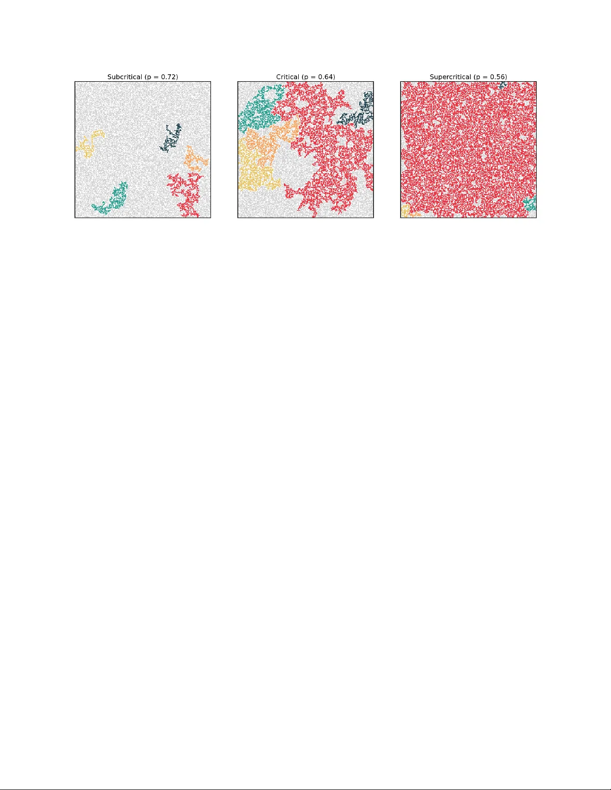
Authors: David Beck-Tiefenbach, Robin Kaiser
Sto c hastic Sandpiles with Uniform T oppling Rule on the Line Da vid Bec k-Tiefenbac h, Robin Kaiser Marc h 18, 2026 Abstract W e consider the sto c hastic sandpile mo del with uniform toppling rule on the integer line. During a uniform toppling, with probabilit y 1 / 3 one particle is sent to the righ t of the toppled v ertex, with probabilit y 1 / 3 one particle is sen t to the left, and with probab ility 1 / 3 t wo particles are sent out, one to the righ t and one to the left. W e calculate exactly the stationary distribution of the stochastic sandpile Mark ov chain with this toppling rule on finite, connected subsets of the in tegers, and show that the infinite volume limit exists and is equal to the Dirac measure of the full configuration. F or this end, we analyze where the excess mass leav es the system, when stabilizing the full configuration plus one additional particle on finite, connected subsets of the in tegers. Keywor ds: sto c hastic sandpiles, ab elian, stationary distribution, infinite v olume limit, uniform toppling, sandpile gambler’s ruin, hole probabilities, line. 2020 Mathematics Sub ject Classification. 60J10, 60K35. 1 In tro duction In 1987, P er Bak, Chao T ang and Kurt Wiesenfeld in tro duced the abelian sandpile mo del in [BTW87, BTW88]. Originally known under the name Bak-T ang-Wiesenfeld mo del, it was the first disco vered dynamical system that reached a critical state on its own, without further fine-tuning of external parameters; a concept kno wn as self-organized criticality . Deepak Dhar later analyzed the mo del further, and show ed that the toppling dynamics are ab elian [Dha90], which led him to coin the term ab elian sandpile mo del . In the ab elian sandpile mo del, the toppling op erations are deterministic, where up on toppling of a v ertex particles are sent out along every adjacent edge to the neighbouring vertices. The only source of randomness thus comes from the c hoice of the initial configuration and the placemen t of the particles. Therefore, a natural generalization of the mo del is to allo w the toppling op erations themselv es to b e random outcomes. That is, up on toppling a v ertex, particles are distributed at random among the neighbours of the toppled vertex. This generalization is kno wn as the sto chastic sandpile mo del . In this manuscript, we w ant to analyze the sto c hastic sandpile mo del on the integer line, where the toppling operations are giv en as the uniform topplings . During a uniform toppling, ev ery possibility of sending out one particle along ev ery adjacent edge is equally lik ely . That is, on the line, when 1 toppling a vertex, with probabilit y 1 / 3 a single particle is either sen t to the right or the left, and with probabilit y 1 / 3 t wo particles are sen t out, one to the right and one to the left. More sp ecifically , we analyze the sto chastic sandpile Markov chain on finite line segments. The sto c hastic sandpile Mark ov chain evolv es by adding a particle at a uniformly c hosen random lo ca- tion, and then stabilizing the resulting sandpile configuration. F or the deterministic counterpart, the ab elian sandpile Mark ov chain, it is known that the stationary distribution will alw a ys b e uni- form on the recurrent sandpile configurations on any finite graph with a sink [Dha90, HLM + 08]. F urthermore, for the ab elian sandpile Mark o v c hain, we can describ e the eigenv ectors via the so-called multiplic ative harmonic functions [JLP19], which can b e used to pro v e the cut-off phe- nomenon on the t wo-dimensional integer grid [HJL19]. It has even b een shown that the infinite v olume limit exists on Z d [AJ04], and a sufficen t condition for the existence of the infinite volume limit has b een found for arbitrary graphs in [J ´ 12, JW14]. Also the density of the infinite v olume limit has b een calculated on Z 2 [Pri94, PP10, PPR11, KW15, KW16], as w ell as the Sierpi ´ nski gask et graph [HKSH25]. W e refer the reader to [J ´ 18] for an introduction to the ab elian sandpile mo del and a collection of further results on the mo del. F or the sto c hastic sandpile Marko v chain, on the other hand, results concerning the stationary distribution or its infinite volume limit are more meagre. In [CMS13], a combinatorial description of the recurren t sandpiles is given for the p -toppling rule, which is similar to the uniform toppling rule of the curren t manuscript. In [CF26] an exact sampling algorithm for the stationary distribution is describ ed, yet again for a different toppling rule, where on all graphs the toppling threshold is 2. F or the uniform toppling rule on finite line segmen ts, w e are able to fully describe the set of recurren t sandpiles, as well as the stationary distribution. W e are also able to show the existence of the infinite volume limit on the integers. Our main results are describ ed in the following theorem. Theorem 1.1. L et for a, b ∈ Z with a < 0 < b denote by µ sto ch a,b the stationary distribution of the sto chastic sandpile Markov chain with uniform toppling rule on the set [[ a, b ]] := { a, a + 1 , ..., b − 1 , b } , wher e the outside is identifie d as the sink. (USS1) It holds that µ sto ch a,b ( 1 [[ a,b ]] ) = 1 2 + 1 2( | a | + b + 2) , wher e 1 [[ a,b ]] denotes the ful l c onfigur ation with one p article at every vertex of [[ a, b ]] . (USS2) The stationary distribution µ sto ch a,b is uniform on the vac ant c onfigur ations. That is, for al l j ∈ [[ a, b ]] it holds that µ sto ch a,b ( 1 [[ a,b ]] − δ j ) = 1 2( | a | + b + 2) , wher e δ j is the c onfigur ation with one p article at j , and 0 everywher e else. (USS3) The infinite volume limit of the stationary distributions on the line exists and is e qual to the Dir ac me asur e of the ful l c onfigur ation on Z , i.e. lim [[ a,b ]] ↑ Z µ sto ch a,b = δ 1 Z . Her e, the limit denotes the uniform we ak limit, that is, for al l se quenc es ( a n ) n ∈ N ∈ Z N < 0 and ( b n ) n ∈ N ∈ Z N > 0 with lim n →∞ a n = −∞ , and lim n →∞ b n = ∞ , 2 and al l finite subsets A ⊆ Z it holds that lim n →∞ µ sto ch a n ,b n ( η | A = 1 A ) = 1 . Theorem 1.1 shows a remark able difference b et ween the sto c hastic sandpile stationary distribution, and its deterministic coun terpart, the stationary distribution of the ab elian sandpile mo del. F or the ab elian sandpile mo del, it is w ell-established, that on any finite graph with a sink v ertex, the stationary distribution of the corresp onding ab elian sandpile Marko v chain is uniform on all recurren t configurations. Despite the symmetries of the uniform toppling rule, the b eha viour of the sto c hastic sandpile Mark ov chain is far from uniform, in fact, it puts half of its total weigh t on the full configuration, and th us seems to fav or an abundance of particles. How ev er, restricted to only the v acant configurations missing one particle, the stationary distribution of the sto c hastic sandpile model still remains uniform. The pro of of Theorem 1.1 relies on analyzing where the excess mass leav es the system up on sta- bilizing the full configuration plus one additional particle. In fact, if w e kno w where the excess mass le a v es our finite subset, and where the v ertices with 0 particles after stabilization o ccur, we can fully calculate the transition probabilities of the sto c hastic sandpile Marko v c hain. With the transition probabilities in hand, we can then analyze the stationary distribution. Outline. In Section 2 w e will in tro duce all the necessary concepts in order to prop erly state and define our mo del, and to prov e Theorem 1.1. Section 3 will b e devoted to pro ving part (USS1) of Theorem 1.1, that is w e sho w that the stationary distribution concen trates around half of its total mass on the full configuration. F or this end, w e will analyze the sandpile gambler’s ruin problem in Subsection 3.1, where w e examine where the excess mass leav es the system up on stabilization of the full configuration plus one additional particle. With the results of the sandpile gam bler’s ruin, w e will then prov e (USS1) in Subsection 3.2. In Section 4, w e will sho w that the infinite volume limit exists and is fully supp orted on the full configuration on Z . Here, we will need to refine our analysis of the sandpile gambler’s ruin, and in vestigate where the v ertices with 0 particles app ear when t w o particles are lost during stabilization of the full configuration plus one additional particle. With these results, w e will then sho w (USS2) in Subsection 4.2, and finally the infinite v olume limit (USS3) will follow in Subsection 4.3. 1.1 Related W orks In this section we wan t to give an ov erview of related works concerning the sto c hastic sandpile mo del and related mo dels. The following is by no means a full and detailed exp osition of works on sto c hastic sandpiles, but merely an ov erview to allow for a prop er placemen t of the current man uscript within the researc h area. F or the sto chastic sandpile mo del and its cousin, the activ ated random walk mo del, we t ypically differen tiate b et ween the driven-dissip ative dynamics and the fixe d-ener gy dynamics. In the driven-dissipativ e dynamics, we consider the mo del on finite graphs with designated sink, and keep adding and stabilizing the configuration until it reaches an equilibrium state. In contrast, for the fixed-energy dynamics, we add to every vertex of our graph a random n um b er of particles, and then try to stabilize the resulting initial configuration in finite time. A p opular conjecture, 3 the density c onje ctur e , claims, that the stationary density of driv en-dissipative dynamics coincides with the critical density of the fixed-energy dynamics. Sto c hastic Sandpiles. F or the sto c hastic sandpile mo del, several random toppling op erations, differen t from the uniform topplings of this man uscript, ha ve b een considered b efore. In [Man91], a mo del is studied, where instead of a toppling threshold, the system is driven b y a hard repulsion of t wo different types of particles which cannot co-exist at the same lo cation. In [CMS13], a toppling rule similar to the uniform toppling is introduced. F or a fixed parameter p ∈ [0 , 1], up on toppling a vertex, for each edge adjacent to the toppled vertex indep endently of the other edges, a particle is sent out along the edge with probabilit y p . [Sel24] analyzes the com binatioral asp ect of this p -toppling on complete graphs, and in [SZ25] a similar analysis is done on complete bipartite graphs. W e w ant to emphasize here, that the dynamics of the uniform toppling rule coincide with p -topplings for p = 1 / 2 . Y et another toppling rule is inv estigated in [HHRR22], where it is shown that the critical density on the integers is strictly b elo w 1, proving a conjecture by Rolla and Sidora vicius [RS12]. Here, a v ertex is declared unstable if it is o ccupied b y more than 2 particles, up on which a toppling lets t wo particles perform a random walk step to the neighbours of the toppled v ertex. It has b een sho wn in [CFT24], that the critical density is strictly b elo w 1 in higher dimensions as w ell. Acitv ated Random W alks. Activ ated random w alks are a sto c hastic net work, where activ e particles p erform a random w alk until they either fall asleep, or reach a designated sink v ertex and are remov ed from the system. Should tw o particles o ccup y the same v ertex at the same time, b oth particles b ecome active again and contin ue p erforming random w alks indep enden tly . See [Rol15, LL24] for a nice o verview of the topic and some related research questions. F or activ ated random walks, it has also b een sho wn that the critical density is strictly less than 1 on the Euclidean lattice in arbitrary dimensions [AFG24]. In the driven-dissipativ e dynamics, also b ounds on the mixing time ha ve b een derived and an exact sampling algorithm for the stationary distribution has b een pro ven [LL24]. Also the density conjecture has b een pro ven to hold true in dimension one [HJJ24]. Activ ated random walks are b elieved to b elong to the same universalit y class as the sto c hastic sandpile mo del considered in [HHRR22, CFT24], whic h highlights a deep connection b et ween these t wo mo dels [L¨ ub04]. 2 Preliminaries In this section w e will define the sto chastic sandpile mo del and collect all results necessary to prov e Theorem 1.1. Uniform T oppling Rules. Let a, b ∈ Z with a < b and consider the set [[ a, b ]] := { a, a + 1 , ..., b − 1 , b } . F or every v ∈ [[ a, b ]] we consider a random v ariable L v taking v alues in Z [[ a,b ]] with the follo wing distribution P ( L v = δ v − 1 − δ v ) = P ( L v = δ v +1 − δ v ) = P ( L v = δ v +1 + δ v − 1 − 2 δ v ) = 1 3 . 4 Here, δ i for i ∈ [[ a, b ]] denotes the Dirac delta function δ i : [[ a, b ]] → Z , j 7→ ( 1 , j = i 0 , else , and δ i is constantly 0 if i / ∈ [[ a, b ]] . W e call L v the uniform toppling or the uniform toppling rule at v , and we call the collection of toppling rules ( L v ) v ∈ [[ a,b ]] the uniform toppling rules on the line segmen t [[ a, b ]]. Notice that topplings at a and b ha ve the chance to remov e a particle from the system, w e will th us refer to the outside as the sink v ertex of the line segment [[ a, b ]] . Sto c hastic Sandpiles. Let a, b ∈ Z with a < b . F urthermore, let for every v ∈ [[ a, b ]] an i.i.d. sequence of random toppling instruction ( L i v ) i ∈ N b e given, where L 1 v ∼ L v . Here ” ∼ ” denotes that the tw o random v ariables are equal in distribution. A sandpile c onfigur ation on [[ a, b ]] is a function η : [[ a, b ]] → Z , that assigns to every vertex of the line segmen t the num ber of particles that is placed at that vertex. Giv en a vertex v ∈ [[ a, b ]], w e say that η is unstable at v , if η ( v ) ≥ 2. W e say the sandpile η is unstable if it is unstable at some v ertex v ∈ V , and stable otherwise. Giv en a sandpile configuration η , stabilization of the sandpile is then defined in the follo wing manner. Set η 0 := η and let u 0 b e the constant 0 function on [[ a, b ]]. W e call u 0 the o dometer function. If η is already stable at every vertex, then the pro cess immediately terminates. Otherwise, c ho ose among the unstable vertices one vertex uniformly at random, and denote the c hoice by v 1 . Then we set η 1 = η 0 + L u 0 ( v 1 )+1 v 1 , u 1 = u 0 + δ v 1 . In w ords, we add a realization of the toppling rule at vertex v 1 to the sandpile configuration and incremen t the o dometer function by 1 at v 1 . If now for some n ∈ N the configuration η n is stable at all vertices, then the pro cess terminates. Otherwise, c ho ose one vertex uniformly at random from all unstable vertices and set η n +1 = η n + L u n ( v n +1 )+1 v n +1 , u n +1 = u n + δ v n +1 , where v n +1 is the c hosen v ertex. This stabilization will even tually terminate for every initial sandpile configuration η . Lemma 2.1 (Stabilization is W ell-Defined) . F or al l initial sandpile c onfigur ations η 0 : [[ a, b ]] → Z , ther e exists almost sur ely an N ∈ N such that η N is stable at al l vertic es. Pr o of. Assume the con trary , that is there exists some configuration η 0 whic h do es not stabilize. Since [[ a, b ]] is finite, there exists a v ertex v ∈ [[ a, b ]] which topples infinitely often. Since L v has p ositiv e probabilit y of sending a particle to either the left or the right, b oth v − 1 and v + 1 receive an infinite amount of particles from v . And b ecause in ev ery step we c ho ose the toppled v ertex uniformly at random, also v − 1 and v + 1 m ust topple infinitely often. W e th us see inductively that all vertices in [[ a, b ]] m ust topple infinitely often, whic h means that also a topples infinitely often. Ho wev er, since toppling at a has p ositiv e probabilit y of reducing the total 5 n umber of particles in the system by 1, an infinite amoun t of particles is lost during stabilization. Ho wev er, η 0 starts with only a finite amoun t of particles, th us we arrive at a con tradiction. This means, that all η 0 m ust stabilize in finitely many steps almost surely . Giv en a sandpile configuration η , w e will denote b y η ◦ the final stabilized configuration. Notice that in the sto c hastic sandpile model, η ◦ is a random v ariable, that is the outcome of the stabilization is itself already random, given that the initial configuration was unstable. Ab elian Prop ert y of T opplings. An imp ortan t prop ert y of the sto c hastic sandpile mo del is, that the order in whic h we topple our vertices do es not influence the final result. F ormally , this means that if w e ha ve tw o unstable vertices v , w ∈ [[ a, b ]], if w e first topple at v and then at w the final configuration will hav e the same la w as if we first toppled at w and then at v . This follo ws directly from the fact that topplings are defined as additions of random columns, i.e. ( η + L i v ) + L j w ∼ ( η + L j w ) + L i v , for all v , w ∈ V and i, j ∈ N and all sandpile configuration η . The ab elian nature of the toppling op erations allo ws us to c ho ose the order in whic h w e topple the unstable vertices during stabilization of a giv en sandpile configuration η , that is, we do not necessarily need to c ho ose the next toppled v ertex uniformly among the curren tly unstable v ertices. W e will rep eatedly mak e use of the ab elian prop ert y throughout this pap er, b y first stabilizing a giv en sandpile configuration in some finite subset A ⊆ [[ a, b ]], b efore we stabilize it fully on the whole line segment [[ a, b ]] . Sto c hastic Sandpile Mark ov Chain. Using the stabilization dynamics of sto c hastic sandpiles, w e can define for all a, b ∈ Z with a < b a Marko v c hain, which takes v alues in the set of stable sandpiles on [[ a, b ]] . Let ( X a,b n ) n ∈ N b e an i.i.d. sequence of random v ariables that are uniformly distributed on [[ a, b ]] . Let further η 0 b e some initial, stable sandpile configuration. W e then define the sto c hastic sandpile Mark ov chain via η n +1 = ( η n + δ X a,b n ) ◦ , that is, in every time step we add an additional particle at a uniformly c hosen lo cation, and then stabilize the configuration. W e call this Mark ov c hain the sto chastic sandpile Markov chain on [[ a, b ]]. It is not hard to see, that the set of recurrent sandpiles is giv en as R a,b := { 1 [[ a,b ]] } ∪ { 1 [[ a,b ]] − δ j : j ∈ [[ a, b ]] } , where 1 [[ a,b ]] denotes the full configuration on [[ a, b ]] that has one particle at every v ertex. W e will further denote by µ stoch a,b the stationary distribution of this Mark ov chain supp orted on R a,b . Infinite V olume Limit. By the infinte volume limit of stationary measures we mean the uniform w eak limit of the stationary measures on the finite line segments [[ a, b ]]. That is, we sa y that the infinite v olume limit exists and is equal to some measure µ supported on the set { η : Z → { 0 , 1 }} , if for all sequencese ( a n ) n ∈ N and ( b n ) n ∈ N with ∀ n ∈ N : a n < 0 < b n , and lim n →∞ a n = −∞ , and lim n →∞ b n = ∞ , 6 it holds for all finite subsets A ⊆ Z and all configurations s : A → { 0 , 1 } that lim n →∞ µ stoch a n ,b n ( η | A = s ) = µ ( η | A = s ) . That is, all finite marginals of the stationary measures must conv erge to the finite marginals of µ , indep enden tly of our choice for ( a n ) n ∈ N and ( b n ) n ∈ N . W e will denote this limit by lim [[ a,b ]] ↑ Z µ stoch a,b = µ. 3 Concen tration Phenomenon of the Stationary Distribution In this section w e will sho w that the stationary distribution of the sto c hastic sandpile Mark ov c hain on finite, connected subsets of the in tegers concen trates almost half its total w eight on the full configuration. F or ease of readability , w e will throughout this section only w ork on the sets of the form C n := { 1 , ..., n } for n ∈ N . As an y finite, connected subset of Z can b e obtained from simply shifting a set C n of suitable length, all the results of this section will carry ov er to arbitrary finite, connected subsets of the in tegers. W e will then denote the stationary distribution of the sto c hastic sandpile Marko v c hain on C n with uniform toppling rule by µ stoch n . The idea of this section will b e to first analyze what happ ens during stabilization of the configuration ( 1 C n + δ j ) for j ∈ C n . More precisely , we wan t to find out the probabilities of losing exactly one particle during stabilization - either through the left side or the right side - or of losing t wo particles, necessarily then through b oth sides. With these probabilities, w e can then find the transition probabilities of the sto chastic sandpile Mark ov c hain to the full configuration, which we can then utilize to prov e the concentration phe- nomenon (USS1). 3.1 Sandpile Gambler’s Ruin In order to analyze the transition probabilities to the full configuration 1 C n , we m ust precisely trac k where the excess mass exits the system when stabilizing the configuration 1 C n + δ j for some j ∈ C n . Recall from Section 2 that the toppling rules ( L v ) v ∈ C n are defined such that particles sen t outside of C n are remov ed. T o rigorously count these lost particles, let us define for eac h toppling L i v the indicator v ariables ∆ L ( L i v ) ∈ { 0 , 1 } and ∆ R ( L i v ) ∈ { 0 , 1 } , whic h equal 1 if the toppling op eration sends a particle to v − 1 or v + 1, respectively . Giv en an initial configuration η 0 , let u : C n → N 0 denote the final o dometer function up on stabi- lization. The total num b er of particles that exit the system through the left b oundary (0) and the righ t b oundary ( n + 1) are giv en by the random v ariables: N L = u (1) X i =1 ∆ L ( L i 1 ) , N R = u ( n ) X i =1 ∆ R ( L i n ) . W e are in terested in the even t where exactly one particle is lost during stabilization, stabilizing to the full configuration 1 C n . 7 Definition 3.1 (Sandpile Gam bler’s Ruin Probabilities) . F or n ∈ N and k ∈ C n , we define the pr ob ability of exactly one p article exiting thr ough the left b oundary up o n stabilizing 1 C n + δ k as: l n ( k ) := P ( 1 C n + δ k ) ◦ = 1 C n , N L = 1 , N R = 0 . A nalo gously, we define r n ( k ) as the pr ob ability that exactly one p article exits thr ough the right b oundary ( N L = 0 , N R = 1 ), and b n ( k ) as the pr ob ability that exactly two p articles exit the system ( N L = 1 , N R = 1 ). F or completeness, w e extend the domain of these functions to the boundaries by setting l n (0) = 1, l n ( n + 1) = 0, and similarly r n (0) = 0, r n ( n + 1) = 1 as well as b n (0) = b n ( n + 1) = 0 . Lemma 3.1 (Recurrence Relation) . F or n ∈ N and k ∈ C n , the pr ob abilities ( l n ( k )) n ∈ N ,k ∈ C n satisfy the r e curr enc e r elation l n ( k ) = 1 3 l n ( k − 1) + l n ( k + 1) + l n − k (1) l n ( k − 1) , with b oundary c onditions l n (0) = 1 and l n ( n + 1) = 0 . Pr o of. Consider the first toppling of the unstable vertex k in the configuration η 0 = 1 C n + δ k . With probability 1 / 3, the particle is sent to k − 1, resulting in the configuration 1 C n + δ k − 1 . The probabilit y of exactly one particle subsequently exiting left is, by definition, l n ( k − 1). Similarly , with probability 1 / 3, the particle is sent to k + 1, yielding 1 C n + δ k +1 and a left-exit probability of l n ( k + 1). With probabilit y 1 / 3, the split toppling occurs, yielding the configuration η 1 = 1 C n − δ k + δ k − 1 + δ k +1 . By the Ab elian prop erty of the sto chastic sandpile model, the final stabilized configuration is indep enden t of the order of subsequent topplings. W e ma y therefore choose to stabilize the sub- segmen t { k + 1 , . . . , n } first. In order for the global condition N R = 0 to hold, this sub-stabilization m ust not eject any particles to the righ t b oundary n + 1. Thus, the single excess particle at k + 1 m ust exit the sub-segmen t to its left, falling in to the hole at k . This indep enden t sub-stabilization b eha v es iden tically to a system of size n − k with a particle added at relative p osition 1. This even t o ccurs with probability l n − k (1). Conditional on this ev ent o ccurring, the hole at k is filled, and the righ t sub-segment is fully stabilized at 1 { k +1 ,...,n } . The remaining unstable configuration on C n is exactly 1 C n + δ k − 1 . The probabilit y that the stabilization of this remaining configuration results in a single left exit is l n ( k − 1). The joint probability of this split sequence is therefore l n − k (1) l n ( k − 1). Summing the probabilities of these three mutually exclusive initial toppling outcomes yields the recurrence. Prop osition 3.1 (Explicit Solution of the Sandpile Gam bler’s Ruin) . F or al l n ∈ N and k ∈ C n , the pr ob abilities of exactly one p article exiting the left or right b oundary, or exactly two p articles exiting, ar e given r esp e ctively by: l n ( k ) = ( n − k + 1)( n − k + 2) ( n + 1)( n + 2) , r n ( k ) = k ( k + 1) ( n + 1)( n + 2) , b n ( k ) = 2 k ( n − k + 1) ( n + 1)( n + 2) . Pr o of. W e prov e this by defining the explicit sequence g n ( k ) := ( n − k + 1)( n − k + 2) ( n + 1)( n + 2) , 8 and sho wing that it uniquely satisfies the recurrence relation established in Lemma 3.1. W e first sho w that the recurrence relation uniquely determines the l n ( k ) b y induction on the system size n . F or the base case n = 1, the v alue l 1 (1) = 1 3 , is determined by the b oundary conditions. Assume that the probabilities are uniquely determined for all system sizes m < n . F or system size n , the recurrence equation from Lemma 3.1 defines a tridiagonal linear system for the unknown v ariables ( l n ( k )) k ∈ C n , where the co efficien ts dep end on the uniquely determined v alue l n − k (1). Be- cause these co efficien ts are sub-sto c hastic, the underlying matrix is irreducibly diagonally dominan t. Therefore, the linear system is non-singular, guaran teeing that the solution for size n is unique. Th us, an y sequence satisfying the recurrence and b oundary conditions must be the true probabilit y ( l n ( k )) k ∈ C n . W e will no w verify that our prop osed function g n satisfies the recurrence. The b oundary conditions are trivially satisfied: g n (0) = ( n + 1)( n + 2) ( n + 1)( n + 2) = 1 and g n ( n + 1) = 0 ( n + 1)( n + 2) = 0 . T o sho w that the recurrence itself is satisfied, we substitute the function g n in to the righ t hand side of the recurrence equation from Lemma 3.1. F or brevity set m = n − k . By the definition of our prop osed sequence, the split-term ev aluates to g m (1) = ( m − 1 + 1)( m − 1 + 2) ( m + 1)( m + 2) = m ( m + 1) ( m + 1)( m + 2) = m m + 2 . Substituting the function g into the recurrence equation of Le mma 3.1 no w yields 1 3 g n ( k − 1) + g n ( k + 1) + g m (1) g n ( k − 1) = 1 3( n + 1)( n + 2) ( m + 2)( m + 3) + m ( m + 1) + m m + 2 ( m + 2)( m + 3) = 1 3( n + 1)( n + 2) ( m 2 + 5 m + 6) + ( m 2 + m ) + ( m 2 + 3 m ) = 1 3( n + 1)( n + 2) 3 m 2 + 9 m + 6 = 3( m + 1)( m + 2) 3( n + 1)( n + 2) = g n ( k ) , as desired. Since g n ( k ) satisfies the recurrence and the solution to the recurrence equation must b e unique, we obtain l n ( k ) = g n ( k ) for all k ∈ C n as well. This finishes the inductive step and thus pro ves the closed-form expression of the probabilities ( l n ( k )) n ∈ N ,k ∈ C n . By symmetry of the uniform toppling rules, the probability of a right exit is given by r n ( k ) = l n ( n − k + 1). Substituting this into our pro v en form ula immediately v erifies the closed-form expression of right-exits. Finally , observe that the probabilit y of losing exactly tw o particles is b n ( k ) = 1 − l n ( k ) − r n ( k ) for all n ∈ N and k ∈ C n . Substituting the explicit expressions for l n ( k ) and r n ( k ) gives b n ( k ) = 2 k ( n − k + 1) ( n + 1)( n + 2) , as desired. 9 Remark 3.1 (Namesake of the Sandpile Gam bler’s Ruin) . We chose to c al l the pr oblem analyze d in this se ction the Sandpile Gambler’s Ruin , not only due to its lo ose r esemblanc e of the classic al gambler’s ruin pr oblem, but b e c ause the classic al gambler’s ruin pr oblem c an b e r e alize d as an analo gue statement for a differ ent toppling rule. Consider for n ∈ N and every i ∈ C n the r andom toppling distribution L SR W i given by P ( L SR W i = δ i − 1 ) = P ( L SR W i = δ i +1 ) = 1 2 . That is, up on toppling any vertex, exactly one p article is sent to the right or left with e qual pr ob ablity. If we now stabilize the ful l c onfigur ation plus one additional p article with this toppling rule, the exc ess p article wil l p erform a simple r andom walk on C n until it either le aves thr ough the left or right side of C n . A nalyzing the pr ob abilities of these two events is known as the Classic al Gambler’s Ruin pr oblem. 3.2 Concen tration on the F ull Configuration With the results on the sandpile gambler’s ruin from Subsection 3.1, we can no w find the transition probabilities to the full configuration. W e will do so in the following lemma. Lemma 3.2 (T ransition Probabilities to F ull Configuration) . L et n ∈ N and c onsider the tr ansition matrix P n of the sto chastic sandpile Markov chain on the set C n . Then: 1. F or al l j ∈ C n it holds that P n ( 1 C n − δ j , 1 C n ) = n + 2 3 n . 2. The ful l c onfigur ation moves to itself with pr ob ability given by P n ( 1 C n , 1 C n ) = 2 3 . Pr o of. W e will first analyze the transition probabilities of the v acant configurations to the full configuration. So let n ∈ N and j ∈ C n , and consider the transition from ( 1 C n − δ j ) to 1 C n . Every step of the sto c hastic sandpile Mark ov chain consists of first placing a particle at a uniformly chosen lo cation in C n . If the particle is placed at vertex j , then the hole at j is filled and we mov ed to the full configuration. This even t contributes a probability of 1 /n to the transition probability . Secondly , if the additional particle is placed at a v ertex i ∈ C n with i < j , i.e. it is placed to the left side of the 0, then w e can first stabilize the configuration ( 1 C n − δ j + δ i ) on the v ertices { 1 , ..., j − 1 } . During this stabilization, if w e w ant the final stable configuration to b e the full configuration 1 C n , exactly one particle m ust leav e the set { 1 , ..., j − 1 } , and it m ust do so through the right side. This corresp onds to the sandpile gam bler’s ruin probability r j − 1 ( i ). W e th us arriv e at a con tribution to the transition probability of 1 n j − 1 X i =1 r j − 1 ( i ) = 1 n j − 1 X i =1 i ( i + 1) 3 j ( j + 1) = ( j − 1) j ( j + 1) 3 nj ( j + 1) = j − 1 3 n , where w e ha ve used the closed-form expression of r j − 1 ( i ) as obtained in Prop osition 3.1. 10 Finally , if the particle is placed to the righ t side of j , we obtain through analogue arguments the con tribution to the transition probability given by 1 n n − j X i =1 l n − j ( i ) = 1 n j − 1 X i =1 ( n − j − i + 1)( n − j − i + 2) 3( n − j + 1)( n − j + 2) = ( n − j )( n − j + 1)( n − j + 2) 3 n ( n − j + 1)( n − j + 2) = n − j 3 n . If w e no w combine all of these three contributions to the transition probabilit y , w e obtain P n ( 1 C n − δ j , 1 C n ) = 1 n + j − 1 3 n + n − j 3 n = n + 2 3 n . Let us now consider the transition probability of the full configuration to itself. F or this even t to o ccur, if a particle is placed at some vertex i ∈ C n , w e m ust then sent out exactly one particle during the stabilization of the configuration ( 1 C n + δ i ), either through the left or the right. The probabilit y of this ev ent is again giv en b y the sandpile gam bler’s ruin as l n ( i ) + r n ( i ) = 1 − b n ( i ) . Using no w again the closed-form expressions obtain in Prop osition 3.1 we obtain P n ( 1 C n , 1 C n ) = 1 n n X i =1 1 − b n ( i ) = 1 − 1 n n X i =1 2 i ( n − i + 1) ( n + 1)( n + 2) = 1 − 1 3 = 2 3 . With these transition probabilities, w e can no w prov e (USS1) from Theorem 1.1. W e will do so in the follo wing prop osition, which will b e phrased on C n . Prop osition 3.2 (Stationary Probability of F ull Configuration) . F or al l n ∈ N it holds that µ sto ch n ( 1 C n ) = 1 2 + 1 2( n + 1) . Pr o of. Let n ∈ N . By the definition of stationary measures we obtain µ stoch n ( 1 C n ) = µ stoch n ( 1 C n ) P n ( 1 C n , 1 C n ) + n X i =1 µ stoch n ( 1 C n − δ i ) P n ( 1 C n − δ i , 1 C n ) . (1) Using Lemma 3.2 we hav e n X i =1 µ stoch n ( 1 C n − δ i ) P n ( 1 C n − δ i , 1 C n ) = n X i =1 µ stoch n ( 1 C n − δ i ) n + 2 3 n = n + 2 3 n n X i =1 µ stoch n ( 1 C n − δ i ) = n + 2 3 n 1 − µ stoch n ( 1 C n ) . Using this in Equation (1) together with the v alue of P n ( 1 C n , 1 C n ) from Lemma 3.2 we obtain µ stoch n ( 1 C n ) = n + 2 3 n + n − 2 3 n µ stoch n ( 1 C n ) . 11 After rearranging this equation we then see 2 n + 2 3 n µ stoch n ( 1 C n ) = n + 2 3 n , from whic h w e finally arriv e at µ stoch n ( 1 C n ) = 1 2 + 1 2( n + 1) , whic h completes our pro of. 4 Infinite V olume Limit In this section, we wan t to show that the infinite v olume limit of stationary distributions on finite line segments exists, and that it is given b y the Dirac measure of the full configuration on the in tegers. F or this end, w e need to get a handle on the stationary probabilties of the v acant config- urations, where exactly one vertex has 0 particles, whereas all the other v ertices hav e 1 particle. It turns out, that we can not only obain suitable b ounds for the stationary probabilities of the v acant configurations, but w e can in fact calculate the stationary distribution on finite line segmen ts exactly . T o do so, we need to refine our analysis of the sandpile gambler’s ruin from Section 3.1. So far, we hav e only found the probabilities of losing exactly one particle, either to the left or to the right, or of losing tw o particles during stabilization of the full configuration plus one additional particle. In order to gain a grasp on the transition probabilities to v acan t configurations - whic h are needed to obtain the stationary distribution - w e ho wev er need to find out, where the v ertex with 0 particles is up on losing tw o particles in the stabilization. W e will take a similar approach as w e did in Section 3.1, that is, we will first find a recurrence equation for the hole probabilities - whic h are the probabilities for the lo cation of the vertex with 0 particles - which we will then solv e to obtain the desired probabilities. This time, the recurrence equation will b e more complicated than the one from 3.1, how ev er it can still b e solv ed with a closed-form solution. W e will calculate the hole probabilites via a suitable recurrence equation in Section 4.1, which w e will then use to calculate the stationary distribution on v acan t configurations in Section 4.2. Finally , we can use the results to prov e the infinite volume limit (USS3) in Section 4.3. 4.1 Hole Probabilities Throughout this section, w e will again work on C n for ease of readabilit y . The results carry ov er to arbitrary line segments [[ a, b ]] for a, b ∈ Z with a < b . When the stabilization of 1 C n + δ i loses exactly t wo particles, the resulting configuration is missing exactly one particle, that is, there will b e a single v ertex with 0 particles on it. W e will denote this vertex as a hole . T o determine the transition probabilities of the Mark ov chain, w e must precisely track the spatial lo cation of this newly created hole. Definition 4.1 (Hole Probabilit y) . F or n ∈ N and i, j ∈ C n , we define h j n ( i ) as the pr ob ability that stabilizing 1 C n + δ i r esults in a single hole lo c ate d exactly at j : h j n ( i ) := P ( 1 C n + δ i ) ◦ = 1 C n − δ j . 12 In order to solv e for h j n ( i ), w e establish t wo distinct recurrence relations b y decomposing the domain in to sub-segments and applying the ab elian prop ert y . Lemma 4.1 (Hole Recurrence Relations) . F or n ≥ 2 , the hole pr ob abilities satisfy the fol lowing r elations. F or i < n , we have the bulk r e curr enc e: h j n ( i ) = r n − 1 ( i ) h j n ( n ) + j − 1 X x =1 h x n − 1 ( i ) h j − x n − x ( n − x ) + h j n − 1 ( i ) r n − j ( n − j ) . F or i = n , we have the b oundary r e curr enc e: h j n ( n ) = ( 1 3 h j n ( n − 1) + 1 3 h j n − 1 ( n − 1) if j < n, 1 3 h n n ( n − 1) + 1 3 l n − 1 ( n − 1) if j = n. Pr o of. W e pro ve the bulk recurrence b y first stabilizing the sub-segment { 1 , . . . , n − 1 } . If exactly one particle exits this sub-segmen t to the left, the configuration becomes 1 C n and no hole is formed. If one particle exits to the right, it lands on n , yielding the configuration 1 C n + δ n , which subse- quen tly forms a hole at j with probability h j n ( n ). Here, the even t to send the particle to vertex n has probabilt y r n − 1 ( i ) . If tw o particles exit the sub-segment, a hole is formed at some x ∈ { 1 , . . . , n − 1 } and the right- exiting particle lands on n . This even t con tributes a probabilit y of h x n − 1 ( i ). W e must now stabilize the configuration on the sub-segmen t { x + 1 , . . . , n } . Crucially , if x > j , the hole at x acts as an absorbing b oundary . The stabilization of the righ t segmen t can emit at most one particle to the left; if it do es, it fills the hole at x , resulting in the fully occupied configuration 1 C n , with p oten tially a hole at some v ertex in the set { x + 1 , . . . , n } . Th us, instability cannot propagate left ward past x to create a hole at j < x . If x < j , the righ t segmen t acts as a system of size n − x and m ust indep enden tly form a hole at relative p osition j − x , giving the sum ov er x < j . If x = j , the hole is already in the correct p osition, so the right segment must simply eject its excess particle to the righ t without filling j , whic h con tributes a probabilit y of r n − j ( n − j ). Summing these m utually exclusiv e tra jectories yields the bulk recurrence equation. T o prov e the boundary recurrence equation, w e examine the first toppling at n . A right topple exits the system, stabilizing to 1 C n , which has no hole. A left topple mov es the particle to n − 1, yielding a remaining probability of h j n ( n − 1) to form a hole at the desired lo cation j . A split toppling creates a hole at n and an excess particle at n − 1. F or j < n , stabilizing { 1 , . . . , n − 1 } must then create a hole at j and eject a particle to the right to fill n , which is an ev ent with probability h j n − 1 ( n − 1). F or j = n , the sub-segment m ust not eject a particle righ t, so it must exit left, yielding the probabilit y l n − 1 ( n − 1). If w e again sum all of the mutually exclusiv e probabilities that can o ccur as explained ab o v e, w e obtain th us the b oundary recurrence equation. W e are now equipp ed to state the main result of this subsection: the spatial lo cation of the hole is uniformly distributed across the domain. Prop osition 4.1 (Uniformit y of the Hole) . F or al l n ∈ N and i, j ∈ C n , the pr ob ability of a hole forming at j is indep endent of j and is given by: h j n ( i ) = b n ( i ) n = 2 i ( n − i + 1) n ( n + 1)( n + 2) . 13 Pr o of. W e prov e this b y showing that g j n ( i ) := b n ( i ) n uniquely satisfies the recurrence relations of Lemma 4.1. W e first sho w that the b oundary and bulk recurrence relations uniquely determine the entire se- quence of probabilities. W e pro ve this b y induction on n . The base case n = 1 is uniquely determined by the toppling rules. Assume the sequence is uniquely determined for all system sizes m < n . F or system size n , ev aluating the bulk recurrence at n − 1 yields h j n ( n − 1) = r n − 1 ( n − 1) h j n ( n ) + K j , where K j := j − 1 X x =1 h x n − 1 ( n − 1) h j − x n − x ( n − x ) + h j n − 1 ( n − 1) r n − j ( n − j ) , dep ends only on systems of size m < n and the lo cation of the hole j , and is therefore fixed. Substituting this into the b oundary recurrence yields a linear equation of the form h j n ( n ) = 1 3 r n − 1 ( n − 1) h j n ( n ) + K j + C j , where j < n : C j := 1 3 h j n − 1 ( n − 1) , C n := 1 3 l n − 1 ( n − 1) , is another fixed constan t independent of the hole probabilities of system size n . Because the co efficien t r n − 1 ( n − 1) / 3 is strictly less than 1, this equation has a strictly unique scalar solution for h j n ( n ). With the b oundary v alue uniquely fixed, the bulk recurrence explicitly and uniquely determines the remaining v alues h j n ( i ) for i < n . Th us, if g j n ( i ) satisfies the recurrences, then g j n ( i ) = h j n ( i ) for all n ∈ N and all i, j ∈ C n . W e will now verify that our prop osed function ( g j n ( i )) i,j ∈ C n satisfies the b oundary recurrence. The left-hand side of the equation simplifies to g j n ( n ) = b n ( n ) n = 2 n n ( n + 1)( n + 2) = 2 ( n + 1)( n + 2) . No w, calculating the righ t-hand side for j < n gives 1 3 g j n ( n − 1) + g j n − 1 ( n − 1) = 1 3 4( n − 1) n ( n + 1)( n + 2) + 2( n − 1) ( n − 1) n ( n + 1) = 1 3 4( n − 1) + 2( n + 2) n ( n + 1)( n + 2) = 1 3 6 n n ( n + 1)( n + 2) = 2 ( n + 1)( n + 2) . Similarly , the right-hand side for j = n gives 1 3 g n n ( n − 1) + l n − 1 ( n − 1) = 1 3 4( n − 1) n ( n + 1)( n + 2) + 2 n ( n + 1) = 2 ( n + 1)( n + 2) . This sho ws that ( g j n ( i )) i,j ∈ C n satisfies the b oundary recurrence. 14 Next, w e will verify that our prop osed function also satisfies the bulk recurrence. W e substitute g in to the right-hand side for i < n . Notice that by definition, g x n − 1 ( i ) do es not dep end on x . Th us, w e can factor it out of the sum S j := P j − 1 x =1 g x n − 1 ( i ) g j − x n − x ( n − x ) to obtain S j = b n − 1 ( i ) n − 1 j − 1 X x =1 2( n − x ) ( n − x )( n − x + 1)( n − x + 2) = b n − 1 ( i ) n − 1 j − 1 X x =1 2 n − x + 1 − 2 n − x + 2 = b n − 1 ( i ) n − 1 2 n − j + 2 − 2 n + 1 , Com bining S j with g j n − 1 ( i ) r n − j ( n − j ), giv es S j + g j n − 1 ( i ) r n − j ( n − j ) = b n − 1 ( i ) n − 1 2 n − j + 2 − 2 n + 1 + n − j n − j + 2 = b n − 1 ( i ) n − 1 n − j + 2 n − j + 2 − 2 n + 1 = b n − 1 ( i ) n − 1 n − 1 n + 1 = 2 i ( n − i ) n ( n + 1) 2 . Finally , adding r n − 1 ( i ) g j n ( n ) w e see that the right-hand side of the bulk recurrence simplifies to i ( i + 1) n ( n + 1) 2 ( n + 1)( n + 2) + 2 i ( n − i ) n ( n + 1) 2 = 2 i n ( n + 1) 2 ( n + 2) h i + 1 + ( n − i )( n + 2) i = 2 i n ( n + 1) 2 ( n + 2) h n 2 + 2 n + 1 − i ( n + 1) i = 2 i ( n + 1)( n − i + 1) n ( n + 1) 2 ( n + 2) = 2 i ( n − i + 1) n ( n + 1)( n + 2) = g j n ( i ) , as desired. Since ( g j n ( i )) i,j ∈ C n satisfies b oth recurrences, and the solution to the recurrences is unique, w e obtain h j n ( i ) = g j n ( i ) for all n ∈ N and all i, j ∈ C n , concluding the pro of. Corollary 4.1 (T ransition Probabilities to V acant Configurations) . L et P n denote the tr ansition matrix of the sto chastic sandpile Markov chain on the r e curr ent c on figur ations of C n for n ∈ N . The pr ob abilities of tr ansitioning to the vac ant c onfigur ations ar e given by P n ( 1 C n , 1 C n − δ i ) = 1 3 n for al l i ∈ C n , P n ( 1 C n − δ j , 1 C n − δ i ) = 1 3 n for i = j, P n ( 1 C n − δ i , 1 C n − δ i ) = n − 1 3 n for al l i ∈ C n . Pr o of. W e will go through the three different transition probabilities of Corollary 4.1. Firstly , observe for i ∈ C n that the Mark ov chain transitions from the sandpile 1 C n to 1 C n − δ i , if w e add a particle uniformly at random at some site x ∈ C n and the subsequen t stabilization forms a hole at i . That is, P n ( 1 C n , 1 C n − δ y ) = 1 n n X x =1 h i n ( x ) = 1 n n X x =1 b n ( x ) n , where the second equality follo ws from Prop osition 4.1. Recall from the pro of of Lemma 3.2 that P n x =1 b n ( x ) = n/ 3. Thus, the transition probabilit y simplifies to P n ( 1 C n , 1 C n − δ i ) = 1 n 2 n 3 = 1 3 n , 15 as desired. Secondly , supp ose we start at 1 C n − δ j and transition to a hole at i < j for i, j ∈ C n . This requires adding a particle at some x < j , and that the sub-segment { 1 , . . . , j − 1 } loses tw o particles during stabilization to form a new hole at i . That is, P n ( 1 C n − δ j , 1 C n − δ i ) = 1 n j − 1 X x =1 h i j − 1 ( x ) = 1 n j − 1 X x =1 b j − 1 ( x ) j − 1 = 1 n ( j − 1) j − 1 3 = 1 3 n , where we again used Prop osition 4.1 and the iden tity P n x =1 b n ( x ) = n/ 3. The case i > j can b e treated analogously . Finally , for all i ∈ C n , the hole remains at i if w e add a particle at x < i and the left sub-segment sends one particle to the left, or if we add a particle at x > i and the right sub-segmen t exits one particle to the right. Summing these con tributions yields P n ( 1 C n − δ i , 1 C n − δ i ) = 1 n i − 1 X x =1 l i − 1 ( x ) + n X x = i +1 r n − i ( x − i ) ! . Using the identit y P m x =1 l m ( x ) = m 3 , this ev aluates to P n ( 1 C n − δ i , 1 C n − δ i ) = 1 n i − 1 3 + n − i 3 = n − 1 3 n , whic h completes the pro of. 4.2 Stationary Distribution on V acant Configurations In this section, w e will use the results on hole probabilities from Section 4.1 to calculate the stationary distribution on the v acan t configurations. That is, we will pro ve (USS2) from Theorem 1.1. Let us again consider the graph C n for some n ∈ N . W e hav e already found the transition probabilities to the v acan t configurations in Corollary 4.1, w e can no w use these results for the stationary probabilities. Prop osition 4.2 (Stationary Probabilities of V acan t Configurations ) . L et n ∈ N and c onsider the stationary distribution µ sto ch n of the sto chastic sandpile Markov chain on C n . F or al l v ∈ C n it holds that µ sto ch n ( 1 C n − δ v ) = 1 2( n + 1) , that is, the stationary distribution is uniform when r estricte d to the vac ant c onfigur ations. Pr o of. Let n ∈ N and v ∈ C n . Similarly to the pro of of Prop osition 3.2 w e use the definition of stationarit y to obtain µ stoch n ( 1 C n − δ v ) = µ stoch n ( 1 C n ) P n ( 1 C n , 1 C n − δ v ) + n X i =1 µ stoch n ( 1 C n − δ i ) P n ( 1 C n − δ i , 1 C n − δ v ) . (2) F rom Corollary 4.1 together with Prop osition 3.2 w e obtain µ stoch n ( 1 C n ) P n ( 1 C n , 1 C n − δ v ) = 1 2 + 1 2( n + 1) 1 3 n . 16 Using Corollary 4.1 we also obtain v − 1 X i =1 i = v µ stoch n ( 1 C n − δ i ) P n ( 1 C n − δ i , 1 C n − δ v ) = 1 3 n n X i =1 i = v µ stoch n ( 1 C n − δ i ) = 1 3 n 1 2 − 1 2( n + 1) − µ stoch n ( 1 C n − δ v ) , as w ell as µ stoch n ( 1 C n − δ v ) P n ( 1 C n − δ v , 1 C n − δ v ) = n − 1 3 n µ stoch n ( 1 C n − δ v ) . Reinserting this in Equation (2) w e obtain the equation µ stoch n ( 1 C n − δ v ) = 1 3 n + n − 2 3 n µ stoch n ( 1 C n − δ v ) , whic h we can solv e for µ stoch n ( 1 C n − δ v ) to obtain (2 n + 2) µ stoch n ( 1 C n − δ v ) = 1 ⇒ µ stoch n ( 1 C n − δ v ) = 1 2( n + 1) , whic h concludes the pro of. Since all sets of the form [[ a, b ]] for a, b ∈ Z with a < 0 < b are simply translated versions of the set C | a | + b +1 , this also shows (USS2) from Theorem 1.1. 4.3 Pro of of the Infinite V olume Limit In this section, w e are finally ready to prov e the existence of the infinite volume limit as stated in (USS3). F or the prov e, we will use the results on the stationary distribution from (USS1) and (USS2). Pr o of of (USS3) fr om The or em 1.1. Consider arbitrary sequences ( a n ) n ∈ N and ( b n ) n ∈ N with ∀ n ∈ N : a n < 0 < b n , and lim n →∞ a n = −∞ , and lim n →∞ b n = ∞ . F urthermore, let A ⊆ Z b e any finite subset of the integers. Let us now c ho ose some n 0 ∈ N such that A ⊆ [[ a n , b n ]] , for all n > n 0 , whic h w e can do since the set A is assumed to b e finite. W e now see for n > n 0 µ stoch a n ,b n ( η | A = 1 A ) = X i ∈ A µ stoch a n ,b n ( 1 [[ a n ,b n ]] − δ i ) = | A | 2( | a n | + b n + 2) . Sending n to infinity we thus obtain lim n →∞ µ stoch a n ,b n ( η | A = 1 A ) = 1 − lim n →∞ | A | 2( | a n | + b n + 2) = 1 , whic h shows lim [[ a,b ]] ↑ Z µ stoch a,b = δ 1 Z , where the limit is in the uniform w eak sense. 17 Figure 1: The graph illustrates the a verage density ρ G ( p ) for p -topplings at certain v alues of p , where G = [[1 , 100]] 2 is a b o x with 10000 vertices. W e can see that the density seems to b e linearly deca ying as w e increase the v alue of p . 5 Conclusion In this paper, w e were able to fully calculate the stationary distribution of sto c hastic sandpiles with the uniform toppling rule on finite line segments, as w ell as establish the existence of the infinite v olume limit on the integers. W e w ant to conclude this work, by addressing some interesting questions suitable for further research efforts. Monotonicit y of the Density . W e ha ve sho wn that the stationary distribution for the uniform toppling rule concentrates around half of its total mass on the full configuration on finite line segmen ts. It seems unlik ely that a similar concentration phenomenon o ccurs on more complicated graphs, ho wev er, w e b eliev e that the a verage density of the stationary distribution will alwa ys b e strictly larger in the uniform toppling case. Consider a finite graph G = ( V ∪ { s } , E ) with designated sink v ertex s . W e consider p -topplings on G , where up on toppling a vertex v ∈ V , for each edge adjacent to v , we decide indep enden tly of the other edges to sent out a particle via the edge with probabilit y p . Should a particle land at s , it is remov ed from the system. Notice that for p = 1 w e obtain the ab elian sandpile mo del, and for p = 1 / 2 all p ossible topplings are equally lik ely . Let no w denote b y µ ( p ) G the stationary distribution of the sto c hastic sandpile Mark ov chain with the p -toppling rule. Let us no w define the a verage density as ρ G ( p ) := E p X v ∈ V η ( v ) | V | , 18 Figure 2: The figure depicts the height 3 cluster of typical samples of the stationary distribution of sto c hastic sandpiles with p -topplings on a b o x of side length 200 for the sub critical and sup ercritical regime, as well as for a v alue of p close to the critical regime. The five largest clusters are highlighted in color, the remaining clusters are depicted in gray . where E p denotes the exp ectation with resp ect to the stationary measure µ ( p ) G . Our first question concerns the b ehaviour of the a verage density ρ G . Conjecture 5.1 (Monotonicit y of the Av erage Density) . F or al l p 1 , p 2 ∈ [0 , 1] with p 1 < p 2 it holds that ρ G ( p 1 ) > ρ G ( p 2 ) , that is, the aver age density ρ G is strictly monotonic al ly de cr e asing in p . In fact, it would already b e in teresting to sho w, that the abelian sandpile mo del has the smallest a verage density . Conjecture 5.2 (Minim um Attained by Ab elian Sandpiles) . F or al l p ∈ [0 , 1) it holds that ρ G ( p ) > ρ G (1) . In Figure 1 we hav e simulated p -topplings on a finite tw o-dimensional b o x, and our results further seem to verify the conjectured monotonicity . P ercolation of Heigh t 3 V ertices. W e ha ve also simulated ho w a t ypical sample of the stationary distribution for p -topplings lo oks on finite b o xes in the t wo-dimensional grid. W e refer to Figure 2 for an illustration of such samples for differen t v alues of p . Consider for n ∈ N the stationary distribution with p -topplings µ ( p ) n on a square b ox [[1 , n ]] 2 , where particles are lost when sen t outside of the b o x. F urthermore, denote for a given sandpile configuration η the set of height 3 v ertices by T n ( η ) := { v ∈ [[1 , n ]] 2 : η ( v ) = 3 } . Our sim ulations suggest that, as we mak e p smaller, the typical size of the set T n ( η ) increases. In fact, for v alues of p that are close to 1, there is only a sp oradic num b er of height 3 vertices. Ho wev er, as we decrease p , even tually the set T n ( η ) starts to connect the left boundary of the b ox with the right b oundary , that is, it p ercolates. 19 Figure 3: The graph shows the probabilit y of finding a cluster of height 3 v ertices spanning from the right side of a b o x of side length L = 120 to the left side of the b o x. Our sim ulations suggest that the phase transition occurs when the a verage densit y of heigh t 3 v ertices is equal to the critical Bernoulli site p ercolation threshhold on Z 2 . Conjecture 5.3. Ther e exists p c ∈ (0 , 1) such that for al l p < p c we have that µ ( p ) n ( Ther e exists a p ath in T n ( η ) that c onne cts the left and right b oundary ) n →∞ − − − → 1 , and for al l p > p c µ ( p ) n ( Ther e exists a p ath in T n ( η ) that c onne cts the left and right b oundary ) n →∞ − − − → 0 . In Figure 3, we hav e plotted the p ercolation probability against the v alue of p , and it seems that there is a sharp decline around the v alue p ≈ 0 . 64 . 20 Single-Source Sandpiles. Consider sto c hastic sandpiles with uniform topplings on the in tegers Z . Our final question concerns the shap e w e obtain when w e place n ∈ N vertices at the origin, and then stabilize the configuration. Our sim ulations strongly suggest the following conjecture. Conjecture 5.4. L et us denote by D n the set of topple d vertic es in the stabilization of ( nδ 0 ) on the inte gers. Then P [ − (1 − ε ) n 2 , (1 − ε ) n 2 ] ⊆ D n ⊆ [ − (1 + ε ) n 2 , (1 + ε ) n 2 ] n →∞ − − − → 1 , for al l ε > 0 . In fact, it would b e in teresting to also consider the limit shap e of the single-source mo del on other graphs, suc h as Z d for d ≥ 2, or for different toppling rules, such as the p -topplings as previously describ ed. F unding Information. This researc h was funded in part by the Austrian Science F und (FWF) 10.55776/P34713. References [AF G24] Amine Asselah, Nicolas F orien, and Alexandre Gaudilli` ere. The critical densit y for activ ated random walks is alw ays less than 1. Ann. Pr ob ab. , 52(5):1607–1649, 2024. [AJ04] Siv a R. A threya and An tal A. J´ arai. Infinite volume limit for the stationary distribution of abelian sandpile mo dels. Comm. Math. Phys. , 249(1):197–213, 2004. [BTW87] P er Bak, Chao T ang, and Kurt Wiesenfeld. Self-organized criticalit y: An explanation of the 1/f noise. Phys. R ev. L ett. , 59:381–384, Jul 1987. [BTW88] P er Bak, Chao T ang, and Kurt Wiesenfeld. Self-organized criticalit y . Phys. R ev. A (3) , 38(1):364–374, 1988. [CF26] Concetta Campailla and Nicolas F orien. Sto c hastic Sandpile Mo del: exact sampling and complete graph. arXiv e-prints , 2026. [CFT24] Concetta Campailla, Nicolas F orien, and Lorenzo T aggi. The critical density of the Sto c hastic Sandpile Mo del. arXiv e-prints , Octob er 2024. [CMS13] Y ao-ban Chan, Jean-F ran ¸ cois Marck ert, and Thomas Selig. A natural sto c hastic ex- tension of the sandpile mo del on a graph. J. Combin. The ory Ser. A , 120(7):1913–1928, 2013. [Dha90] Deepak Dhar. Self-organized critical state of sandpile automaton mo dels. Phys. R ev. L ett. , 64(14):1613–1616, 1990. [HHRR22] Christopher Hoffman, Yiping Hu, Jacob Ric hey, and Douglas Rizzolo. Active Phase for the Stochastic Sandpile on Z. arXiv e-prints , December 2022. [HJJ24] Christopher Hoffman, T obias Johnson, and Matthew Junge. The density conjecture for activ ated random walk. arXiv e-prints , 2024. arXiv.2406.01731. 21 [HJL19] Rob ert D. Hough, Daniel C. Jerison, and Lionel Levine. Sandpiles on the square lattice. Comm. Math. Phys. , 367(1):33–87, 2019. [HKSH25] Nico Heizmann, Robin Kaiser, and Ecaterina Sav a-Huss. Average height for Ab elian sandpiles and the lo oping constan t on Sierpi ´ nski graphs. Comput. Appl. Math. , 44(5):P a- p er No. 227, 27, 2025. [HLM + 08] Alexander E. Holro yd, Lionel Levine, Karola M´ esz´ aros, Y uv al Peres, James Propp, and Da vid B. Wilson. Chip-firing and rotor-routing on directed graphs. In In and out of e quilibrium. 2 , v olume 60 of Pr o gr. Pr ob ab. , pages 331–364. Birkh¨ auser, Basel, 2008. [J ´ 12] A. A. J´ arai. Ab elian sandpiles: an ov erview and results on certain transitive graphs. Markov Pr o c ess. R elate d Fields , 18(1):111–156, 2012. [J ´ 18] An tal A. J´ arai. Sandpile mo dels. Pr ob ab. Surv. , 15:243–306, 2018. [JLP19] Daniel C. Jerison, Lionel Levine, and John Pike. Mixing time and eigenv alues of the ab elian sandpile Marko v chain. T r ans. Amer. Math. So c. , 372(12):8307–8345, 2019. [JW14] An tal A. J´ arai and Nicol´ as W erning. Minimal configurations and sandpile measures. J. The or et. Pr ob ab. , 27(1):153–167, 2014. [KW15] Richard W. Ken yon and Da vid B. Wilson. Spanning trees of graphs on surfaces and the in tensity of lo op-erased random walk on planar graphs. J. Amer. Math. So c. , 28(4):985– 1030, 2015. [KW16] Adrien Kassel and David B. Wilson. The lo oping rate and sandpile density of planar graphs. Amer. Math. Monthly , 123(1):19–39, 2016. [LL24] Lionel Levine and F eng Liang. Exact sampling and fast mixing of activ ated random w alk. Ele ctr on. J. Pr ob ab. , 29:Paper No. 184, 20, 2024. [L ¨ ub04] Sven L ¨ ub ec k. Universal scaling b eha vior of non-equilibrium phase transitions. Interna- tional Journal of Mo dern Physics B , 18(31-32):3977–4118, January 2004. [Man91] S S Manna. Two-state mo del of self-organized criticality . Journal of Physics A: Math- ematic al and Gener al , 24(7):L363, apr 1991. [PP10] V ahagn P oghosyan and Vyatc hesla v Priezzhev. The problem of predecessors on span- ning trees. A cta Polyte chnic a , 51, 10 2010. [PPR11] V ahagn S Poghosy an, Vy atchesla v B Priezzhev, and Philipp e Ruelle. Return probabilit y for the lo op-erased random walk and mean height in the ab elian sandpile mo del: a pro of*. Journal of Statistic al Me chanics: The ory and Exp eriment , 2011(10):P10004, o ct 2011. [Pri94] Vy atchesla v B Priezzhev. Structure of tw o-dimensional sandpile. I. heigh t probabilities. Journal of statistic al physics , 74:955–979, 1994. [Rol15] Leonardo T. Rolla. Activ ated random walks. arXiv e-prints , 2015. [RS12] Leonardo T. Rolla and Vladas Sidoravicius. Absorbing-state phase transition for driven- dissipativ e sto c hastic dynamics on Z . Invent. Math. , 188(1):127–150, 2012. 22 [Sel24] Thomas Selig. The stochastic sandpile model on complete graphs. Ele ctr on. J. Combin. , 31(3):P ap er No. 3.26, 29, 2024. [SZ25] Thomas Selig and Hao yue Zhu. Ab elian and stochastic sandpile mo dels on complete bipartite graphs. In WALCOM: algorithms a nd c omputation , volume 15411 of L e ctur e Notes in Comput. Sci. , pages 326–345. Springer, Singap ore, [2025] © 2025. D a vid Beck-Tiefenbach , Universit¨ at Innsbruck, Institut f ¨ ur Mathematik, T ec hnikerstraße 23, A-6020 Innsbruc k, Austria. david.beck-tiefenbach@uibk.ac.at R obin Kaiser , Departemen t of Mathematics, CIT, T echnisc he Univ ersit¨ at M¨ unchen, Boltzmannstr. 3, D-85748 Garching b ei M ¨ unc hen, Germany . ro.kaiser@tum.de 23
Original Paper
Loading high-quality paper...
Comments & Academic Discussion
Loading comments...
Leave a Comment