A Kernel Two-Sample Test Invariant under Group Action with Applications to Functional Data

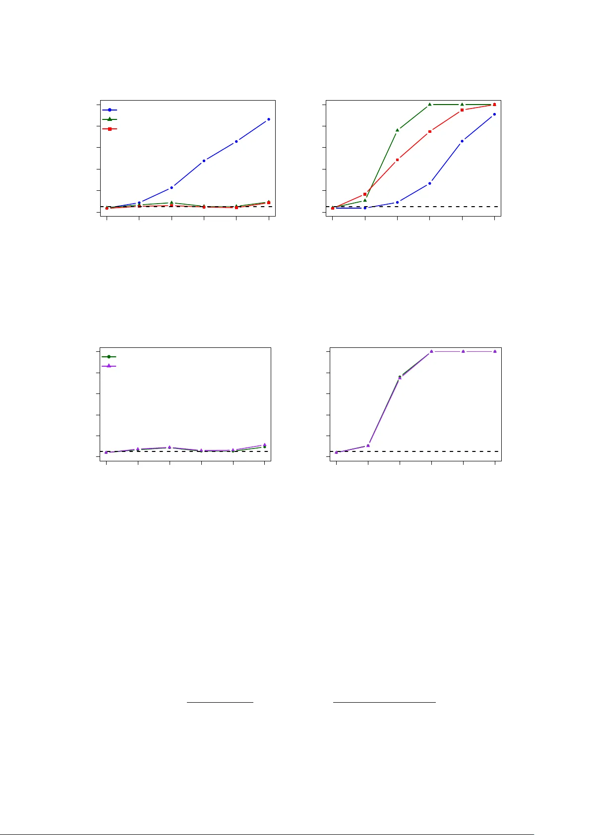
A Kernel Tw o-Sample T est In v arian t under Group Action with Applications to F unctional Data Madison Giacofci ∗ Anouar Meynaoui ∗ Alex P o dgorn y † Abstract W e in tro duce a k ernel-based t wo-sample test for comparing probability distributions up to group actions. Our construction yields in v ariant kernels for locally compact σ -compact groups and extends classical Haar-based approac hes beyond the compact setting. The result- ing in v arian t Maxim um Mean Discrepancy (MMD) test is developed in a general framework where the sample space is assumed to b e P olish. Under natural conditions, the in v arian t k ernel induces a characteristic kernel on the quotient space, ensuring consistency of the as- so ciated MMD test. The metho d is well suited to functional data, where inv ariances suc h as temp oral shifts arise naturally , and its effectiveness is illustrated through simulation studies. 1 In tro duction In many real-w orld applications, the v ariabilit y observed in data is partially explained by n ui- sance transformations. F or functional data, t ypical examples include translations, rotations, scalings, time-shifts, or more general reparametrizations that preserve the underlying conten t of a given observ ation. Such transformations arise naturally in many application domains. F or instance, images representing the same ob ject or scene may differ b y rotations, translations, or changes in scale dep ending on the camera viewp oin t. Similarly , handwritten digits may in- v olve small deformations while still representing the same digit [ 1 ]. In gro wth curve analysis, individuals may exp erience biological ev ents suc h as growth spurts at different ages, producing curv es that are essentially iden tical up to a temp oral reparametrization [ 2 ]. In audio analysis, t wo signals corresp onding to the same sound ma y differ only b y a time shift or b y a change in duration due to recording conditions [ 3 ]. In biomedical signal analysis, electro cardiogram (ECG) signals record the electrical activity of the heart ov er time. Tw o ECG signals may lo ok differen t simply b ecause the heart b eats slightly faster or slow er, whic h shifts the timing of the main p eaks in the signal. In this case, the ov erall pattern remains the same, but it app ears stretched or shifted in time [ 4 ]. In suc h settings, directly comparing the distributions of tw o datasets can b e misleading, since apparent differences may arise solely from nuisance transformations, even when the tw o samples represen t the same underlying phenomenon. This motiv ates the dev el- opmen t of statistical pro cedures that are inv ariant to prescrib ed transformations, so that only meaningful differences b et w een distributions are detected. In this work, we fo cus sp ecifically on the tw o-sample testing problem. Kernel-based tw o-sample tests provide a p o werful and flexible framework for comparing proba- bilit y distributions. In particular, metho ds based on the maxim um mean discrepancy (MMD) ha ve b ecome widely used due to their strong theoretical guaran tees and their ability to handle complex and high-dimensional data [ 5 ]. Ho wev er, standard kernel tw o-sample tests are t ypi- cally sensitive to transformations of the data, ev en though in many applications distributions should b e regarded as equal up to nuisance transformations. A natural wa y to address this issue ∗ Univ ersit´ e Rennes 2, IRMAR, UMR CNRS 6625, Rennes, F rance † Ensai, CNRS, CREST-UMR 9194, Rennes, F rance 1 is to incorp orate inv ariance into the comparison pro cedure through the action of a group on the observ ation space. Under this p erspective, observ ations that differ only b y such transfor- mations are regarded as equiv alen t, and the relev an t ob ject b ecomes the distribution induced on the corresp onding quotien t space. The resulting testing problem is therefore to determine whether t wo distributions remain differen t once these transformations are disregarded. A clas- sical w ay to enforce suc h in v ariance in kernel metho ds consists in a veraging a base k ernel along the transformations of the group. When the group is compact, this a veraging can b e p erformed using the Haar probability measure, leading to kernels that are inv arian t under the prescrib ed transformations. This idea has b een explored in the machine-learning literature [ 6 , 7 , 8 ]. The same a veraging mec hanism also app ears prominently in the theory of data augmentation. In practice, augmentation replaces each observ ation with randomly transformed v ersions. In many pip elines, training pro ceeds b y rep eatedly sampling such transformations. Augmenting inputs and then learning with a kernel method is close ly related to replacing the original k ernel with an augmen tation-av eraged version, obtained b y a veraging the base kernel ov er all pairs of transfor- mations of the tw o inputs. This relationship is made explicit in several works [ 7 , 9 , 10 ]. These connections suggest that augmen tation can be viewed as transforming the underlying distribu- tions b efore comparison. Another related but distinct problem is to test whether the underlying distribution of a sample is in v arian t under the action of a giv en group. The recent w ork of [ 11 ] prop oses k ernel-based tests for this problem when the acting group is compact. Our ob jective is differen t, we instead compare t wo distributions mo dulo a group action, i.e., w e test equality on the quotient space. As mentioned earlier, existing approaches rely on the compactness of the transformation group. In man y situations of practical interest, transformations such as translations or scalings inv olve non-compact groups. F or such groups, the Haar measure is not finite and cannot b e normalized in to a probabilit y measure. As a consequence, the a veraging construction describ ed ab o ve cannot b e applied directly , and extending k ernel-based testing pro cedures to suc h settings requires differen t ideas. Con tributions. Our main con tributions are as follo ws. • In v ariant kernels b ey ond compact groups. W e introduce a w eigh ted a veraging pro- cedure for lo cally compact σ -compact groups, which yields w ell-defined inv ariant k ernels. This extends the classical Haar-integration kernel construction, whic h is limited to com- pact groups [ 6 , 7 ]. In the non-compact setting, it is typically replaced b y quasi-inv ariant surrogates [ 8 ]. • A rigorous in v ariant MMD t w o-sample test. Using these inv ariant kernels, we for- malize an MMD-based inv ariant tw o-sample test. Then, we study its statistical prop erties in a general theoretical framework. In particular, the only assumption on the data space is that it is Polish. • Characteristic k ernels on the quotien t. W e show that the inv ariant kernel induces a k ernel on the quotient space. Under natural conditions, this k ernel is c haracteristic. The asso ciated MMD is therefore zero if and only if the t wo distributions are equal on the quotien t. Consequently , the resulting tw o-sample test is consisten t. Organization of the pap er. Section 2 recalls some background material. In Section 2.1 , w e review basic notions on RKHS and kernels, as w ell as the asso ciated nonparametric t w o- sample tests. In Section 2.2 , we recall basic notions on groups, group actions, and the Haar measure. Section 3 presen ts our inv ariant MMD t w o-sample test. It con tains the main theoretical con tributions of the pap er and discusses practical asp ects of implementing the test. Section 4 presen ts simulation studies on syn thetic signals with temporal shifts. Section 5 illustrates the metho dology on a real-data application to phono cardiogram (PCG) signals. 2 2 Bac kground 2.1 Review on Kernel tw o-sample tests Nonparametric tw o-sample testing is a fundamental problem in statistics, where the aim is to determine whether tw o samples are dra wn from the same underlying probabilit y distribution. Mathematically , assume we ha ve t wo indep endent i.i.d. samples { X i } n i =1 ∼ P , { Y i } m i =1 ∼ Q, where P and Q are probabilit y measures on a measurable space ( X , A ). The tw o-sample problem consists in testing H 0 : P = Q against H 1 : P  = Q. Early nonparametric tw o-sample tests include the Kolmogoro v–Smirnov one [ 12 ], whic h com- pares empirical cumulativ e distribution functions, via the suprem um norm. A ma jor limitation of this test is that it is restricted to one-dimensional data, as its formulation relies on the existence of a natural total ordering of the observ ations. Other classical t wo-sample pro cedures are based on the Cramer–von Mises criterion, whic h replaces the suprem um by an integrated squared dif- ference [ 13 ]. A closely related test is the Anderson–Darling procedure, originally developed in the one-sample setting [ 14 , 15 ] and later extended to the t wo-sample problem [ 16 ], where a weigh t- ing function is introduced in the integrated squared difference. Lik e the Kolmogoro v-Smirnov test, these pro cedures fundamentally exploit univ ariate ordering and therefore do not admit a canonical multiv ariate extension. T o ov ercome these limitations, k ernel-based t wo-sample tests ha ve b een in tro duced. These approaches compare probability distributions b y mapping them in to a Reproducing Kernel Hilb ert Space (RKHS), thereb y reducing the tw o-sample test to the comparison of elemen ts in a Hilb ert space. The discrepancy induced by this embedding leads to the Maximum Mean Discrepancy (MMD), whic h defines a metric on the space of proba- bilit y measures for the so-called characteristic k ernels [ 17 , 5 ]. Kernel-based t w o-sample tests offer several adv antages, including the ability to detect general distributional differences in arbi- trary dimensions, theoretical guaran tees of consistency for characteristic kernels, and flexibilit y through k ernel choice [ 5 ]. Moreo ver, the MMD admits simple empirical estimators with go od statistical prop erties and can b e efficien tly computed in practice. Accordingly , we fo cus on MMD-based testing pro cedures in the remainder of this w ork. Before introducing k ernel-based tw o-sample tests, w e first recall some key notions for their construction. Let X be a non-empty set and let H b e a Hilb ert space of real-v alued functions on X equipp ed with inner pro duct ⟨· , ·⟩ H and norm ∥ · ∥ H . The space H is called a Repro ducing Kernel Hilb ert Space (RKHS) if, for ev ery x ∈ X , the p oin t-ev aluation functional L x : H → R defined by L x ( f ) = f ( x ) is con tinuous. By the Riesz represen tation theorem, this implies that for each x ∈ X there exists a unique elemen t ϕ ( x ) ∈ H such that f ( x ) = ⟨ f , ϕ ( x ) ⟩ H for all f ∈ H , known as the repro ducing prop ert y [ 18 ]. The asso ciated repro ducing kernel is defined as k : X × X → R , k ( x, x ′ ) := ⟨ ϕ ( x ) , ϕ ( x ′ ) ⟩ H , and satisfies k ( · , x ) ∈ H together with f ( x ) = ⟨ f , k ( · , x ) ⟩ H for all f ∈ H . An RKHS is uniquely characterized b y its repro ducing k ernel, and conv ersely ev ery positive definite k ernel defines a unique RKHS. Consequently , we refer to these tw o notions interc hangeably in the follo wing. Bey ond represen ting individual p oin ts x ∈ X in a RKHS, the kernel framew ork also allows probabilit y measures on X to b e embedded as elemen ts of the Hilb ert space via exp ectations of feature maps [ 19 , 20 ]. Given a probability measure P on a measurable space ( X , A ) suc h that E X ∼ P [ p k ( X, X )] < ∞ , its kernel mean embedding is defined as m ( P ) := E X ∼ P [ k ( · , X )] ∈ H . A kernel k is said to b e characteristic if the mean embedding map P 7→ m ( P ) is injective, that is, m ( P ) = m ( Q ) if and only if P = Q . Characteristic kernels therefore ensure that probabilit y distributions are uniquely represen ted b y their mean embeddings in the RKHS, a prop ert y that is crucial for defining distances b etw een distributions based on kernel em b eddings 3 [ 20 ]. Giv en t wo probabilit y measures P and Q on ( X , A ), the Maximum Mean Discrepancy (MMD) associated with a k ernel k is defined as MMD k ( P , Q ) := ∥ m ( P ) − m ( Q ) ∥ H . When the k ernel k is characteristic, this quantit y defines a metric on the space of probability measures, in the sense that MMD k ( P , Q ) = 0 if and only if P = Q [ 5 ]. The tw o-sample problem reduces to testing H 0 : MMD k ( P , Q ) = 0 against H 1 : MMD k ( P , Q ) > 0 . In practice, the MMD k ( P , Q ) is unkno wn and is estimated from the a v ailable samples. Indeed, the MMD admits a closed-form expression in terms of expectations, namely MMD 2 k ( P , Q ) = E X,X ′ ∼ P [ k ( X, X ′ )] + E Y ,Y ′ ∼ Q [ k ( Y , Y ′ )] − 2 E X ∼ P ,Y ∼ Q [ k ( X, Y )] , where all exp ectations are taken ov er indep enden t copies. Replacing these exp ectations by their empirical coun terparts yields an unbiased estimator of MMD 2 k ( P , Q ) in the form of a t w o-sample U-statistic of order t wo. This estimator is given by \ MMD 2 k = 1 n ( n − 1) X i  = i ′ k ( X i , X i ′ ) + 1 m ( m − 1) X j  = j ′ k ( Y j , Y j ′ ) − 2 nm n X i =1 m X j =1 k ( X i , Y j ) . T o construct a level- α test, a natural choice is to reject H 0 for large v alues of \ MMD 2 k b y com- paring it to the (1 − α )-quantile of its distribution under H 0 . In practice, this null quanti le is unkno wn b ecause the distributions P and Q are unknown, and it is therefore estimated either b y a p erm utation pro cedure or by approximating the asymptotic distribution under H 0 . These differen t procedures are describ ed b elo w. The p erm utation pro cedure relies on the fact that the p ooled sample ( X 1 , . . . , X n , Y 1 , . . . , Y m ) is exchangeable under H 0 . Let Z = ( Z 1 , . . . , Z n + m ) denote this p o oled sample with Z i = X i for i ≤ n and Z n + j = Y j for j ≤ m . Under H 0 , the joint distribution of Z is inv ariant under p erm utations of the indices, so that for any p erm utation π of { 1 , . . . , n + m } , the statistic denoted \ MMD 2 k,π and computed with the sample ( Z π (1) , . . . , Z π ( n + m ) ) has the same distribution as the original statistic \ MMD 2 k . One draws B indep enden t p erm utations π 1 , . . . , π B uniformly from the set of all permutations of { 1 , . . . , n + m } , indep enden tly of the data Z , and computes the p erm uted statistics \ MMD 2 k,π b for b = 1 , . . . , B . T ogether with the original v alue \ MMD 2 k , this yields B + 1 exchangeable statistics, and the rejection threshold is defined as the empirical (1 − α )-quantile of these B + 1 v alues [ 21 , 22 ]. The resulting test has non-asymptotic level α under H 0 , a guarantee that follo ws from the permutation test lemma of Romano and W olf based on exchangeabilit y arguments [ 23 , 24 ]. Alternativ e calibration strategies rely on the asymptotic distribution of \ MMD 2 k under the n ull h yp othesis, whic h is given by an infinite w eighted sum of indep enden t c hi-square random v ari- ables [ 5 ]. In practice, th is distribution is t ypically appro ximated either through sp ectral methods or by moment-matc hing with a Gamma distribution [ 25 , 5 ]. In the remainder of the pap er, w e consider the p erm utation pro cedure, whic h pro vides exact finite-sample lev el con trol and non- asymptotic theoretical guarantees. 2.2 Group actions W e briefly review the basic notions from group theory and group actions used throughout this pap er. This discussion is kept concise and emphasizes aspects that are useful for our construc- tions. F or more details on lo cally compact groups, Haar measures, and in tegration on groups, see [ 26 , 27 ]. Groups and Haar measure. A set G equipp ed with a binary operation ∗ : G × G → G is a group if ∗ is asso ciativ e (for all a, b, c in G , ( a ∗ b ) ∗ c = a ∗ ( b ∗ c )), there exists an identit y elemen t 4 e ∈ G (for all a ∈ G , a ∗ e = e ∗ a = a ) and ev ery elemen t of G has an in verse (for all a ∈ G , there exists a − 1 ∈ G such that a ∗ a − 1 = a − 1 ∗ a = e ). F or notational con venience, we write ab instead of a ∗ b . In the following, G is assumed to b e a topological group. That is, a group endo wed with a top ology for which the group op eration ( a, b ) 7→ a ∗ b and the inv ersion a 7→ a − 1 are contin uous. A fundamental result in harmonic analysis states that if G is lo cally compact and Hausdorff, then there exists a nonzero measure λ l on the Borel σ -algebra of G , called a left Haar measure, whic h is inv ariant under left translations. Meaning that, for all g ∈ G and A ⊆ G a measurable set: λ l ( g A ) = λ l ( A ), where g A = { g a | a ∈ A } . The left Haar measure is unique up to a multiplicativ e constan t. Similarly , there exists a unique righ t-inv ariant Haar measure λ r . In the sequel, we consider unimo dular groups, for which the left and righ t Haar measures coincide. W e then refer to λ as the Haar measure, inv ariant under b oth left and righ t translations. Another imp ortan t result states that λ ( G ) is finite if and only if G is compact. In this case, λ can b e normalized in to a probabilit y measure. When G is non-compact (e.g. G = R d ), the Haar measure has infinite total mass. Moreov er, if G is σ -compact, the Haar measure is σ -finite. Group actions, orbits, and quotien t spaces. Let ( X , B ( X )) b e a measurable space. A (left) action of G on X is a mapping φ : G × X → X ( g , x ) 7→ φ g ( x ) , suc h that φ e = id X (the identit y function on X ) and for all g , h ∈ G , φ g h = φ g ◦ φ h . The orbit of a given x in X is defined by [ x ] := { φ g ( x ) | g ∈ G } . W e denote b y X /G := { [ x ] | x ∈ X } the set of all orbits, called the quotien t space. W e also denote b y Π the canonical pro jection from X to X /G , asso ciating to eac h x in X its orbit Π( x ) := [ x ]. By construction, for all g ∈ G , Π ◦ φ g = Π. W e equip X /G with the quotien t σ -algebra defined b y B ( X /G ) := { A ⊆ X /G | Π − 1 ( A ) ∈ B ( X ) } , whic h is the largest σ -algebra on X /G that mak es Π measurable. All probability measures on X /G considered in this pap er are defined on ( X /G, B ( X /G )). Imp ortantly , our theoretical results only rely on this measurable structure and no top ological assumptions on X /G are required. In the follo wing, w e assume that the action φ is join tly measurable with resp ect to the pro duct σ -algebra on G × X . Remark 1. If X is a top olo gic al sp ac e and the action φ is c ontinuous, one may endow X /G with the quotient top olo gy, define d as the finest top olo gy making Π c ontinuous. However, unless additional assumptions (such as pr op erness of the action) ar e imp ose d, this top olo gy may b e p atholo gic al (e.g. non-Hausdorff ). Sinc e our analysis is pur ely me asur e-the or etic, we do not r ely on any top olo gic al pr op erties of X /G . F or further discussion of tr ansformation gr oups and quotient sp ac es (including c onditions such as pr op erness ensuring wel l-b ehave d quotients), se e [ 28 ]. W e present b elow some examples of the space X , the group G and its asso ciated action. • Image rotations. Let X b e a space of images. F or example, we may take X to b e a subspace of functions from R 2 to R . Let G = SO(2) b e the sp ecial orthogonal group in dimension 2, a compact group, defined b y SO(2) := n Q ∈ M 2 ( R ) | Q ⊤ Q = I 2 and det( Q ) = 1 o =  Q θ =  cos θ − sin θ sin θ cos θ  ∈ M 2 ( R )     θ ∈ [0 , 2 π )  , 5 where M 2 ( R ) is the set of 2 × 2 real matrices and I 2 is the identit y 2 × 2 matrix. The group action is defined for all θ in [0 , 2 π ) and x in X b y φ θ ( x ) : u 7→ x ( Q ⊤ θ u ) . The action φ θ corresp onds to rotating the image b y an angle θ around the origin. • Time shifts of p eriodic signals. Consider X to b e a space of T -perio dic signals on R , and let G = R /T Z act by time shifts. More precisely , the group action is defined for all [ τ ] in G and x in X by φ [ τ ] ( x ) : u 7→ x ( u − τ ) . In this case, G is compact. • Time shifts of ap erio dic signals. Let X b e a space of non-p eriodic signals on R , and let G = ( R , +) act on X b y translations. F or all t in G and x in X , the action is giv en by φ t ( x ) : u 7→ x ( u − t ) . In this case, G is non-compact but lo cally compact. 3 In v arian t t w o-sample tests under group actions The aim of this section is to construct a nonparametric t w o-sample test for comparing t wo distri- butions modulo a group action. F or this, w e consider t w o indep enden t i.i.d samples { X i } n i =1 ∼ P and { Y i } m i =1 ∼ Q , where P and Q are probability measures on a measurable space ( X , A ), a uni- mo dular group G endow ed with its Haar measure λ , and a group action φ of G on X . Under the notations and assumptions of Section 2.2 , w e call a G -in v arian t t wo-sample test, the follo wing testing problem H 0 : Π ∗ P = Π ∗ Q against H 1 : Π ∗ P  = Π ∗ Q, (1) where Π ∗ P (resp ectiv ely Π ∗ Q ) denotes the pushforward measure of P (resp ectively Q ) b y Π. The idea here is to compare the distributions P and Q while disregarding the v ariabilit y induced b y the group action, whic h is viewed as a n uisance transformation. While the case of compact groups has b een partially studied in the literature [ 6 , 7 , 8 ], the case of lo cally compact groups remains unexplored. An ob jectiv e of this work is to address this extension. In the compact case, the starting p oint is to consider an a v eraged k ernel ℓ λ : ( x, y ) 7→ Z G Z G ℓ ( φ g ( x ) , φ h ( y )) d λ ( g ) d λ ( h ) , where ℓ is a characteristic kernel on X . This a veraging remov es the information provided by the group’s action and defines a k ernel whose v alues are completely determined by the orbits. F or lo cally compact groups, the k ernel ℓ λ is not alwa ys well-defined, as the Haar measure can b e infinite. In the sequel, we assume that G is a lo cally compact and σ -compact group and that the tw o follo wing assumptions hold. The space X is assumed to b e P olish and the group action φ : G × X → X is jointly measurable. W e also equip the quotient space X /G with the quotien t σ -algebra in tro duced in Section 2.2 . 3.1 W eighting and admissible measures A crucial step in building the test given by ( 1 ) is to b e able to define, for a given probability P on X and a measure ν on G , an av erage of the transformations of P under the action of the group G . If it is w ell-defined, this ν -a v eraged probabilit y is giv en by S ν P := Z G ( φ g ) ∗ P d ν ( g ) , (2) 6 where ( φ g ) ∗ P denotes the pushforw ard measure of P by φ g . W e will show later that when ν = λ is the Haar measure, the testing problem ( 1 ) amoun ts to comparing S ν P and S ν Q . T o remain fully general, we define the ν -av erage of a k ernel ℓ b y ℓ ν : ( x, y ) 7→ Z G Z G ℓ ( φ g ( x ) , φ h ( y )) d ν ( g ) d ν ( h ) . (3) It is clear that S ν P is not alwa ys defined in the case of non-compact groups and for a general measure ν . In what follo ws, w e in tro duce classes of measures on X and G for whic h the ν - a veraged probability in ( 2 ) and the ν -av eraged k ernel in ( 3 ) are well-defined. F or this, w e consider a w eighting function ρ with a sufficien tly fast decay to ensure the in tegrability with resp ect to measures on X and G . W e assume that ρ is a strictly p ositive and b ounded Borel function and we denote by M ( X ) the space of signed measures on ( X , B ( X )) and by M σ ( G ) the space of σ -finite measures on ( G, B ( G )). W e denote by M ρ ( X ) and M ρ ( G ) the follo wing t wo classes of measures M ρ ( X ) :=  µ ∈ M ( X ) : Z X ρ ( x ) d | µ | ( x ) < ∞  , M ρ ( G ) :=  ν ∈ M σ ( G ) : sup x ∈X  Z G ρ ( φ g ( x )) d ν ( g )  < ∞  . Note that the class M ρ ( G ) includes all probabilit y measures on G . More imp ortan tly , for a suit- able choice of the w eighting function ρ and dep ending on the group action under consideration, M ρ ( G ) may also con tain infinite measures, including the Haar measure λ on lo cally compact and σ -compact groups. As stated ab o ve, the role of the w eighting function ρ is precisely to con trol integrabilit y along group orbits, thereb y extending the class of admissible measures on G b ey ond finite measures. Consider now k , a con tinuous, bounded and p ositiv e definite k ernel on X and the w eighted kernel k ρ : ( x, y ) 7→ ρ ( x ) k ( x, y ) ρ ( y ) . Since k is measurable and p ositiv e definite, and ρ is measurable, it follo ws that the k ernel k ρ is measurable and p ositiv e definite on X × X . With these definitions in place, we now provide a sufficient condition ensuring that the ν -a veraged probabilit y S ν P is well-defined. W e then establish a result showing that the distance induced by the w eighted kernel k ρ distinguishes ν -av eraged probabilities. Prop osition 1. L et ν ∈ M ρ ( G ) . F or al l pr ob ability me asur es P ∈ P ( X ) , the aver age d me asur e S ν P := Z G ( φ g ) ∗ P d ν ( g ) is wel l-define d and b elongs to M ρ ( X ) . Prop osition 2. Assume that k is char acteristic on the sp ac e of finite signe d me asur es M f ( X ) . Then, k ρ is char acteristic on M ρ ( X ) . This means that the MMD based on k ρ is able to distinguish a veraged distributions, which is a crucial ingredient for consistency of the inv ariant test. T o estimate MMD k ρ ( S ν P , S ν Q ) from i.i.d. samples dra wn from P and Q , w e first express it as an MMD b et ween P and Q with respect to another kernel. It turns out that this k ernel is precisely the ν -av erage of the k ernel k ρ . 3.2 Av eraged and in v ariant k ernels Let us introduce the av eraged k ernel that will b e used to p erform the G -inv ariant tw o-sample test defined in ( 1 ). The main idea is to build a kernel that compares observ ations only through 7 their b ehavior along group orbits. This is achiev ed by av eraging the weigh ted kernel k ρ o ver the action of the group. Let ν ∈ M ρ ( G ), we define the ν -a veraged kernel k ρ ν as k ρ ν : ( x, y ) 7→ Z G Z G k ρ ( φ g ( x ) , φ h ( y )) d ν ( g ) d ν ( h ) . The integrabilit y conditions enco ded in the definition of M ρ ( G ) ensure that the k ernel k ρ ν is w ell-defined. Indeed, for x, y in X k ρ ν ( x, y ) = Z G Z G k ρ ( φ g ( x ) , φ h ( y )) d ν ( g ) d ν ( h ) = Z G Z G ρ ( φ g ( x )) k ( φ g ( x ) , φ h ( y )) ρ ( φ h ( y )) d ν ( g ) d ν ( h ) ≤ ∥ k ∥ ∞  Z G ρ ( φ g ( x )) d ν ( g )   Z G ρ ( φ h ( y )) d ν ( h )  < + ∞ (4) where ∥ k ∥ ∞ = sup x,y ∈X | k ( x, y ) | . The kernel k ρ ν compares t wo elements x and y b y av eraging similarities b et ween pairs of p oin ts taken from their resp ectiv e orbits. If k is symmetric p ositiv e definite, then k ρ ν is as w ell. This result is shown in the next prop osition, whic h also pro vides a useful interpretation of the feature representation of k ρ ν . Prop osition 3. Assume that k and ρ ar e c ontinuous and b ounde d. L et ν in M ρ ( G ) and Φ ρ : x 7→ k ρ ( x, · ) b e the c anonic al fe atur e map of k ρ . Then, for al l x, y in X , k ρ ν ( x, y ) = ⟨ Φ ρ ν ( x ) , Φ ρ ν ( y ) ⟩ H ρ k , wher e Φ ρ ν : x 7→ Z G Φ ρ ( φ g ( x )) d ν ( g ) . In other wor ds, Φ ρ ν is the c anonic al fe atur e map of k ρ ν . In p articular, k ρ ν is a p ositive definite kernel on X . Prop osition 3 shows that the feature map asso ciated with k ρ ν is obtained by a v eraging the one of k ρ along group orbits. The natural question that arises is the link betw een the mean em b eddings asso ciated with the kernels k ρ and k ρ ν . This result is giv en in the next prop osition. Prop osition 4. Assume that k and ρ ar e c ontinuous and b ounde d. L et ν b e in M ρ ( G ) and P in P ( X ) . Denote by m ρ ν ( P ) the me an emb e dding of P with r esp e ct to k ρ ν , and by m ρ ( S ν P ) the me an emb e dding of S ν P with r esp e ct to k ρ . Then, m ρ ν ( P ) = m ρ ( S ν P ) . Prop osition 4 sho ws that em bedding P with k ρ ν is equiv alent to embedding the a veraged measure S ν P with k ρ . This can also b e interpreted in light of Prop osition 3 . The philosoph y b ehind m ρ ν ( P ) is to embed first and then av erage, whereas that of m ρ ( S ν P ) is to av erage first and then em b ed. These are tw o sides of the same coin. The next corollary is an immediate consequence. Corollary 1. Assume that k and ρ ar e c ontinuous and b ounde d. L et ν in M ρ ( G ) and P , Q in P ( X ) . Then, MMD k ρ ν ( P , Q ) = MMD k ρ ( S ν P , S ν Q ) . Recall that k ρ is characteristic on M ρ ( X ) and, by Prop osition 1 , that S ν P ∈ M ρ ( X ) for every probabilit y distribution P . It follows that MMD k ρ ( S ν P , S ν Q ) = 0 if and only if S ν P = S ν Q . Let us now fo cus on the case ν = λ , where λ denotes the Haar measure. When G is compact, this measure is finite and can therefore b e normalized to a probability measure, namely the 8 uniform distribution on G . In this setting, without further assumptions on λ , b oth the λ - a veraged probability S λ P and the λ -av eraged kernel k ρ λ in ( 2 ) and ( 3 ) are w ell-defined. When G is non-compact, the Haar measure has infinite total mass. How ev er, for a suitable c hoice of the w eighting function ρ , it b elongs to M ρ ( G ). Then, according to Prop osition 1 and Equation ( 4 ), the av eraged probabilities and the av eraged kernel are well-defined, despite the infiniteness of λ . Theorem 1. Assume that k and ρ ar e c ontinuous and b ounde d, and that the Haar me asur e λ b elongs to M ρ ( G ) . L et P , Q in P ( X ) . Then, S λ P = S λ Q if and only if Π ∗ P = Π ∗ Q . The distribution S λ P is obtained by av eraging P uniformly along each group orbit. Because the Haar measure is in v arian t, this av eraging treats all p oin ts in the orbit in the same wa y . As a result, an y information ab out how the mass is distributed inside an orbit disapp ears, and only the total mass assigned to eac h orbit remains. Since Π ∗ P exactly represents this mass on the orbit space, S λ P is completely determined b y Π ∗ P and conv ersely . If ν is not the Haar measure, the av eraging is no longer uniform along the orbits. In that case, the result ma y still dep end on ho w the mass is arranged within eac h orbit, and this corresp ondence with the quotien t distribution no longer holds. Remark 2. The c ondition λ in M ρ ( G ) dep ends on b oth the action and the choic e of ρ . In gener al, ther e is no universal choic e of ρ ensuring it. Consider the c ase wher e φ is the trivial action, namely φ : ( g , x ) 7→ x . If G is non-c omp act, then any weighting function ρ > 0 satisfies Z G ρ ( φ g ( x )) d λ ( g ) = Z G ρ ( x )d λ ( g ) = ρ ( x ) λ ( G ) = + ∞ . This me ans that λ do es not b elong to M ρ ( G ) . At the opp osite extr eme, when G is c omp act, the Haar me asur e is finite. One may simply take ρ ≡ 1 , in which c ase k ρ λ yields the classic al Haar-aver age d invariant kernel. It is also imp ortan t to emphasize that since k ρ λ is constant on orbits, it induces a measurable p ositiv e kernel e k ρ λ on the quotient X /G , defined b y e k ρ λ : ([ x ] , [ y ]) 7→ k ρ λ ( x, y ) . (5) The kernel ˜ k λ is characteristic on the set of pushforw ard measures under Π, namely Π ∗ P ( X ) := { Π ∗ P | P ∈ P ( X ) } . Thanks to Prop osition 1 and Corollary 1 , by using the in v arian t k ernel k ρ λ , one can p erform the MMD tw o-sample test on the quotien t space without ev er ha ving to construct it explicitly . In other words, the testing problem ( 1 ) boils do wn to testing H 0 : MMD k ρ λ ( P , Q ) = 0 against H 1 : MMD k ρ λ ( P , Q ) > 0 . (6) In the next section, we discuss the practical asp ects of its implemen tation. 3.3 In v ariant MMD test in practice Assuming that the kernel k ρ λ is known, a t wo-sample test can b e p erformed based on ( 6 ). T o do so, the MMD is estimated using the unbiased U-statistic intr o duced in Section 2.1 . The rejection threshold is then obtained via the permutation pro cedure. In our setting, the theo- retical v alidit y of this pro cedure still holds. Indeed, the k ernel k ρ λ dep ends only on the orbits through the kernel e k ρ λ in tro duced in ( 5 ). Moreo v er, under H 0 , the p o oled sample of orbits { Π( X 1 ) , . . . , Π( X n ) , Π( Y 1 ) , . . . , Π( Y m ) } is exc hangeable. Consequently , the distribution of the 9 MMD estimator is unc hanged under p erm utations. Therefore, the p erm utation pro cedure yields a v alid level- α test. Practically sp eaking, computing k ρ λ requires ev aluating an integral that is generally in tractable in closed form. T o address this issue, we introduce a pro cedure to appro ximate it for eac h pair ( x, y ) ∈ X 2 . Assume that the Haar measure λ b elongs to M ρ ( G ) for some weigh ting function ρ . W e define the orbit-a veraged weigh t function b y w : x 7→ Z G ρ ( φ g ( x )) d λ ( g ) . F or all x in X , define the measure ν x on G by ν x ( dg ) := ρ ( φ g ( x )) w ( x ) d λ ( g ) . (7) Then, ν x is a probability measure on G . In addition, k ρ λ can b e written as k ρ λ : ( x, y ) 7→ w ( x ) w ( y ) Z G Z G k ( φ g ( x ) , φ h ( y )) d ν x ( g ) d ν y ( h ) . (8) The represen tation ( 8 ) pla ys a key role in appro ximating the kernel k ρ λ for pairs of p oin ts ( x, y ) in X 2 . Indeed, it enables a Monte-Carlo approximation. W e assume that ρ is chosen s o that the normalizing constant w ( x ) is analytically computable or numerically approximable. Note that when G is compact, Remark 2 implies that ρ ≡ 1, w ≡ λ ( G ) and that for all x in X , ν x = λ/λ ( G ). Let { g s } S s =1 and { h s } S s =1 b e i.i.d. samples from ν x and ν y , resp ectively . Then, k ρ λ ( x, y ) can b e approximated by k ρ λ ( x, y ) := e w ( x ) e w ( y ) S 2 S X r =1 S X s =1 k ( φ g r ( x ) , φ h s ( y )) , where e w ( x ) and e w ( y ) are approximations of w ( x ) and w ( y ), resp ectiv ely . Once the k ernel k ρ λ is appro ximated b y k ρ λ , the permutation-based test describ ed in Section 2.1 can b e carried out using samples from P and Q . Obviously , increasing S reduces the approximation error, but results in higher computational cost and memory usage. W e now presen t tw o illustrativ e examples concerning the choice of ρ and the approximation of k ρ λ . Recall that all the theoretical results presen ted in this pap er are stated in a very general setting. The only assumption on X is that it is a P olish space. In particular, it is not required to b e lo cally compact. This generalit y allows us to consider applications in functional data analysis, where observ ations are curves or signals. The Hilb ert space X = L 2 ( I ) of real-v alued square-integrable functions on an interv al I ⊆ R , pro vides a natural and widely used functional framework. A commonly used kernel on L 2 ( I ) is the Gaussian one, defined by k : ( x, y ) 7→ exp  − ∥ x − y ∥ 2 2 2 σ 2  , (9) where ∥ · ∥ 2 denotes the usual L 2 -norm and σ > 0 is a bandwidth parameter. It has recently b een sho wn in [ 29 ] that the Gaussian kernel is c haracteristic on the class of finite measures. Therefore, it constitutes a sound and flexible c hoice for the base k ernel. Time shifts of p erio dic signals. Consider the space of real-v alued 1-p eriodic functions on R whose restriction to [0 , 1] b elongs to L 2 ([0 , 1]), mo dulo equality almost ev erywhere. This functional space is canonically identified with X = L 2 ( S 1 ), where S 1 = R / Z denotes the circle. Let G = ( S 1 , +) and let φ b e the circular shift action φ : G × X → X ( τ , x ) 7→ φ τ ( x ) = x ( · − τ ) . 10 As mentioned earlier, since G is compact, we ha ve ρ ≡ 1. F urthermore, λ can b e iden tified with the Leb esgue measure on [0 , 1), so that λ ( G ) = 1 and ν x is the uniform distribution on S 1 . Then, the Haar-av eraged inv ariant k ernel is defined by k ρ λ : ( x, y ) 7→ Z S 1 Z S 1 k ( φ τ ( x ) , φ ι ( y )) d λ ( τ ) d λ ( ι ) , where k is the Gaussian kernel introduced in ( 9 ). Let { τ s } S s =1 and { ι s } S s =1 b e i.i.d. samples dra wn uniformly from S 1 . Then, k ρ λ ( x, y ) is approximated b y k ρ λ ( x, y ) = 1 S 2 S X r =1 S X s =1 exp  − ∥ x ( · − τ r ) − y ( · − ι s ) ∥ 2 2 2 σ 2  . (10) In practice, the L 2 -norms are replaced b y discretized appro ximations. Time shifts of ap erio dic signals. Consider now the non-perio dic setting where X =  f ∈ L 2 ( R ) | ∥ f ∥ 2 2 ≤ R  , where R > 0. Let G = ( R , +) and let φ : ( τ , x ) 7→ x ( · − τ ) b e the time shift action. Here, G is non-compact and its Haar measure λ is the Leb esgue measure. F or c > 0, define the weigh ting function ρ c b y ρ c : x 7→ Z R x 2 ( u ) exp  − u 2 2 c 2  d u. (11) This functional applies a Gaussian window centered at zero, giving more weigh t to v alues of the signal near the reference time origin. Let c > 0 and x in X . Then, using T onelli’s theorem, we ha ve Z R ρ c ( φ τ ( x )) d λ ( τ ) = Z R Z R x 2 ( u − τ ) exp  − u 2 2 c 2  d u d τ = Z R  Z R x 2 ( u − τ )d τ  exp  − u 2 2 c 2  d u = c √ 2 π ∥ x ∥ 2 2 . Then, sup x ∈X  Z R ρ c ( φ τ ( x )) d λ ( τ )  ≤ c √ 2 π R. In other words, λ b elongs to M ρ c ( G ). Assume now that the function x is discretized ov er an in terv al [ − T / 2 , T / 2] using a uniform grid with p p oin ts x ( t 1 ) , . . . , x ( t p ). The discretized v ersion of ρ c ( φ τ ( x )) is given b y e ρ c ( φ τ ( x )) = T p − 1 p X k =1 x 2 ( t k ) exp  − t 2 k 2 c 2  . This shows that ν x can b e approximated by a mixture Gaussian distribution. In addition, w ( x ) can b e approximated by e w ( x ) = √ 2 π c T p − 1 p X k =1 x 2 ( t k ) . 11 4 Sim ulations W e present a n umerical study illustrating the implementation of the inv ariant MMD test de- v elop ed in this pap er. T o this end, w e consider X = L 2 ( I ), where I is a real interv al. The group action corresp onds to translations along the horizontal axis. Our goal is tw ofold. On the one hand, we empirically verify level control when the t wo distributions differ only through the group action. On the other hand, we assess the pow er when the difference cannot be explained b y a translation. W e consider t wo different settings, a p erio dic one in Section 4.2 and an ap eri- o dic one in Section 4.3 . In b oth settings, we compare the p erformance of the in v arian t test, the align-then-test pro cedure, and the base-k ernel test. 4.1 General setup F or all k ernel-based tests, the test statistic is the unbiased U-statistic MMD estimator recalled in Section 2.1 . In eac h setting, w e sim ulate i.i.d. samples X n = ( X 1 , . . . , X n ) and Y m = ( Y 1 , . . . , Y m ) drawn from P and Q , resp ectiv ely , with n = m = 20. Each exp erimen t is rep eated N rep = 300 times in order to estimate empirical rejection rates. The realizations are discretized on a uniform grid with p = 128 p oin ts ov er an interv al [ a, b ]. In addition, the squared L 2 -norm of a curve x is approximated as ∥ x ∥ 2 2 ≈ b − a p − 1 p X k =1 x 2 ( t k ) . On a discrete grid, the action φ t z = z ( · − t ) is implemen ted b y ev aluating the signal at shifted lo cations t k − t using linear interpolation (with p eriodic wrapping in Exp erimen t 1 and zero padding in Exp erimen t 2). In the main sim ulations, the kernel k ρ λ is appro ximated b y its Mon te Carlo version k ρ λ according to Equation ( 10 ), with sample sizes S = 16. This pro vides a go od trade-off b et ween computational cost and statistical p erformance. Additional numerical sim ulations are conducted with S = 32. The base k ernel k is the Gaussian kernel defined in Equation ( 9 ). The bandwidth σ is chosen at eac h rep etition using the median heuristic applied to the pairwise L 2 -distances of the p ooled sample Z n = ( X 1 , . . . , X n , Y 1 , . . . , Y m ). The rejection threshold is calibrated via the p erm utation pro cedure describ ed in Section 2.1 . T o do so, w e generate uniformly B = 200 random p erm utations { π b } B b =1 of the lab els, compute the p erm uted statistics \ MMD 2 k,π b and estimate the p -v alue as p v al = 1 B + 1 1 + B X b =1 1 n \ MMD 2 k,π b ≥ \ MMD 2 k o ! , where \ MMD 2 k is the U-statistic computed with the original sample Z n . Then, we reject the null h yp othesis whenever p v al ≤ α with α = 0 . 05. Alignmen t baseline. Besides comparing the kernels k and k ρ λ , w e also consider the classical baseline ”align-then-test”. This approac h attempts to remo ve spurious translations b y aligning the curves b efore p erforming the test. T o do so, one defines a reference signal for eac h sample, after which the observ ations are shifted and scaled to b est match it. W e denote by X ref and Y ref the reference signals asso ciated with X n and Y m , resp ectiv ely . In the remainder, these refe rence signals are considered to b e the empirical medoids. F or the sample X n , the reference is defined b y X ref ∈ arg min X i ∈ X n X X j ∈ X n ∥ X i − X j ∥ 2 . Then, each realization X i is shifted by ˆ t i giv en b y ˆ t i ∈ arg min t inf a ∥ X ref − aX i ( · − t ) ∥ 2 . 12 A similar definition holds for Y ref and the same alignment pro cedure is applied. Then, the MMD tw o-sample test is p erformed using the aligned samples and the k ernel k . Suc h alignment pip elines are standard in functional data analysis and signal processing (see, e.g., [ 2 ]). Unlike the in v arian t-kernel approach, this metho d requires estimating nuisance parameters and selecting a reference signal. This may affect its stability when alignment is w eakly identifiable. 4.2 Time shifts of p erio dic signals W e consider a perio dic setting where the observ ations are 2 π -p erio dic, up to m ultiplicative noise. The actions corresp ond to circular shifts on [0 , 2 π ). As in the p erio dic example of Section 3.3 , the acting group G = R / 2 π Z is compact and we take ρ ≡ 1. Data generation. Let X and Y b e the random pro cesses defined by X = γ h 1 ( · − θ 1 ) ε and Y = γ h 2 ( · − θ 2 ) ε, where the amplitude γ is log-normally distributed with log-mean 0 and log-standard deviation σ γ , θ 1 and θ 2 are random phases (taken mo dulo 2 π ) and ε is Gaussian white noise with mean 1 and standard deviation 0.8. The random v ariables γ , θ 1 , θ 2 and the random pro cess ε are indep enden t. The distributions and the functions h 1 , h 2 v ary across sim ulations. They are sp ecified in the corresp onding scenarios b elo w. The sample X n (resp ectiv ely Y n ) is generated according to the distribution of X (resp ectiv ely Y ). Scenario H 0 . In this scenario, w e consider sin usoidal functions h 1 = h 2 = sin, θ 1 ≡ e θ 1 (mo d 2 π ) and θ 2 ≡ e θ 2 (mo d 2 π ) , where e θ 1 (resp ectiv ely e θ 2 ) is Gaussian with mean δ / 2 (resp ectiv ely − δ/ 2) and standard deviation σ θ 1 = 0 . 8 (resp ectiv ely σ θ 2 = 0 . 8). All v alues of δ ranging from 0 to 1 with a step of 0.2 are considered in the sim ulations. With this generating mec hanism, the distributions P and Q differ, but coincide mo dulo translations. In other w ords, Π ∗ P = Π ∗ Q . Scenario H 1 . Let h 1 = sin, h 2 : t 7→ h 1 ( t ) + δ sin(2 t + 0 . 3), θ 1 ≡ e θ 1 (mo d 2 π ) and θ 2 ≡ e θ 2 (mo d 2 π ) , where e θ 1 , e θ 2 are Gaussian with mean 0 and standard deviation σ θ = 0 . 8. In this setting, the distributions differ even after alignment. This means that, Π ∗ P  = Π ∗ Q . Figure 1 represents the empirical rejection rates, with resp ect to δ under the H 0 and H 1 sce- narios. Under H 0 , the in v arian t and alignmen t tests b eha ve well, with lo w rejection rates. Both pro cedures are correctly calibrated, their empirical rejection rates remain close to the nominal lev el α for all v alues of δ . The results obtained with the kernel k are consistent with its theoret- ical construction. Since the original distributions differ, the test based on k detects differences and its p o wer increases with δ . Under the alternative, the three tests hav e increasing p o wer as δ increases. Moreov er, b oth the inv arian t test and the align-then-test pro cedures ac hieve substan tially higher p o w er than the k -based test. Therefore, removing the translation nuisance enhances the ability to capture in trinsic shap e differences b et w een the t wo groups of signals. In addition, except for δ = 0 . 2, the inv ariant test has significantly higher p o w er than the align- then-test baseline. W e also assess the sensitivit y of the results to the appro ximation of k ρ λ . F or this, w e conduct the same exp erimen ts with a larger Monte Carlo budget, namely S = 32. Fig- ure 2 presen ts the corresp onding empirical rejection rates. The results remain quasi-unchanged. This indicates that the b ehavior of the in v arian t test is stable with resp ect to the approximation budget. 13 0.0 0.2 0.4 0.6 0.8 1.0 0.0 0.2 0.4 0.6 0.8 1.0 Null hypothesis δ Empirical rejection rate Base−kernel test Inv ariant test Align−then−test 0.0 0.2 0.4 0.6 0.8 1.0 0.0 0.2 0.4 0.6 0.8 1.0 Alternative hypothesis δ Empirical rejection rate Figure 1: P erio dic case . Empirical rejection rates of the MMD tests based on k , k ρ λ and the align-then-test baseline with resp ect to δ . The approximation budget of k ρ λ is S = 16. Left. P  = Q and Π ∗ P = Π ∗ Q . Righ t. Π ∗ P  = Π ∗ Q . 0.0 0.2 0.4 0.6 0.8 1.0 0.0 0.2 0.4 0.6 0.8 1.0 Null hypothesis δ Empirical rejection rate S = 16 S = 32 0.0 0.2 0.4 0.6 0.8 1.0 0.0 0.2 0.4 0.6 0.8 1.0 Alternative hypothesis δ Empirical rejection rate Figure 2: P erio dic case . Empirical rejection rates of the MMD tests based on k ρ λ with tw o differen t appro ximation budgets. Left. P  = Q and Π ∗ P = Π ∗ Q . Righ t. Π ∗ P  = Π ∗ Q . 4.3 Time shifts of ap erio dic signals W e no w consider an ap erio dic setting in which the signals are observ ed on a finite window, namely [ − 5 , 5]. In this case, the acting group ( R , +) is non-compact and a weigh ting function is required. W e c ho ose a w eigh ting function of the form ρ c defined in Equation ( 11 ), where the selection rule for c is introduced below. Choice of the parameter c . W e prop ose the following heuristic, whic h appears to be robust in practice. Let t = ( t 1 , . . . , t p ) b e the temp oral grid. F or a giv en signal x , w e define the w eighted temp oral mean µ x and v ariance s 2 x as µ ( x ) = P p k =1 t k x 2 ( t k ) P p k =1 x 2 ( t k ) and s ( x ) 2 = P p k =1 ( t k − µ x ) 2 x 2 ( t k ) P p k =1 x 2 ( t k ) . W e then set c to c := median { s i | 1 ≤ i ≤ n + m, and s i > 0 } , 14 where s i = s ( X i ) for 1 ≤ i ≤ n and s i = s ( Y i ) for n + 1 ≤ i ≤ n + m . This rule can be in terpreted as follows. The quan tity s ( x ) measures the temporal disp ersion of the signal energy around its barycen ter. The median is then computed o ver the p ooled sample. This provides a robust scale shared by the tw o groups. As a result, the Gaussian weigh ting is neither ov erly lo calized nor o verly diffuse. Data generation. Let X and Y b e the random pro cesses defined by X = γ h 1 ( · − θ 1 ) ε and Y = γ h 2 ( · − θ 2 ) ε, where the amplitude γ is log-normally distributed with log-mean 0 and log-standard deviation σ γ , θ 1 and θ 2 are random translations and ε is Gaussian white noise with mean 1 and standard deviation 0.8. The random v ariables γ , θ 1 , θ 2 and the random pro cess ε are indep enden t. As in Section 4.2 , the functions and parameters v ary across simulations. The samples X n and Y n are generated according to the distribution of X and Y , resp ectiv ely . Scenario H 0 . In this case, h 1 = h 2 : t 7→ exp( − 2 t 2 ) and θ 1 (resp ectiv ely θ 2 ) is Gaussian with mean δ / 2 (resp ectiv ely − δ / 2) and standard deviation σ θ 1 = 0 . 8 (resp ectiv ely σ θ 2 = 0 . 8). The sim ulations consider v alues of δ ranging from 0 to 1 with incremen ts of 0.2. Similarly to the H 0 case in Section 4.2 , the distributions P and Q are different, but induce the same distribution in the quotient space. Scenario H 1 . Let h 1 : t 7→ exp( − 2 t 2 ) and h 2 = h 1 + δ / 4 × p , where p is the t wo-bump function defined by p : t 7→ exp  − 2( t − 1) 2  + 0 . 4 exp  − ( t + 1) 2 2  . The random v ariables θ 1 , θ 2 are Gaussian with mean 0 and standard deviation σ θ = 0 . 8. Figure 3 shows the empirical rejection rates with resp ect to δ under the H 0 and H 1 scenarios. The results in the ap erio dic setting are similar to those obtained in the p erio dic case. The in v arian t and align-then-test pro cedures remain well calibrated under H 0 and their p o wer increases with δ . The inv ariant test ac hieves the b est performance, follow ed by the align-then-test pro cedure, and then the baseline test. As in the perio dic setting of Section 4.2 , w e assess the sensitivity to the approximation of k ρ λ . Results obtained with S = 32 are presented in Figure 4 and remain essen tially unc hanged. 0.0 0.2 0.4 0.6 0.8 1.0 0.0 0.2 0.4 0.6 0.8 1.0 Null hypothesis δ Empirical rejection rate Base−kernel test Inv ariant test Align−then−test 0.0 0.2 0.4 0.6 0.8 1.0 0.0 0.2 0.4 0.6 0.8 1.0 Alternative hypothesis δ Empirical rejection rate Figure 3: Ap erio dic case . Empirical rejection rates of the MMD tests based on k , k ρ λ and the align-then-test baseline with resp ect to δ . The approximation budget of k ρ λ is S = 16. Left. P  = Q and Π ∗ P = Π ∗ Q . Righ t. Π ∗ P  = Π ∗ Q . 15 0.0 0.2 0.4 0.6 0.8 1.0 0.0 0.2 0.4 0.6 0.8 1.0 Null hypothesis δ Empirical rejection rate S = 16 S = 32 0.0 0.2 0.4 0.6 0.8 1.0 0.0 0.2 0.4 0.6 0.8 1.0 Alternative hypothesis δ Empirical rejection rate Figure 4: Ap eriodic case . Empirical rejection rates of the MMD tests based on k ρ λ with t wo differen t appro ximation budgets. Left. P  = Q and Π ∗ P = Π ∗ Q . Righ t. Π ∗ P  = Π ∗ Q . 5 Real data application W e illustrate our in v arian t tw o-sample test on phono cardiogram (PCG) signals from the public PhysioNet/Computing in Car diolo gy Chal lenge 2016 dataset (a v ailable here ). A phono cardio- gram is an audio recording of the sounds pro duced by the heart o ver successive cardiac cycles. The training set is partitioned into six subsets ( training-a to training-f ). It contains a total of 3126 recordings whose durations range from a few seconds to more than one minute. The signals are collected under heterogeneous conditions, using different sensors and in diverse clin- ical and en vironmental settings. In this application, we restrict our analysis to the training-e subset. Prepro cessing and p erio dic represen tation. All audio files are resampled to a common time grid with 1000 measuremen ts per second. Then, a band-pass filter remo ves very slow trends and rapid fluctuations caused by noise. W e compute a smo othed energy en v elop e of the signal using a sliding RMS (ro ot mean square). Next, we compute the auto correlation of the env elop e. The characteristic cardiac p eriod, denoted b T , is the time lag that maximizes the auto correlation within a plausible heart-rate range. The estimated p erio d is used only to extract a fixed-length segmen t from each recording. This segmen t is treated as one p erio d of a p erio dic signal. F rom eac h file, w e construct a vector using one of the strategies b elo w, illustrated in Figure 5 . S 1 -aligned extraction. The first heart sound, denoted S 1 , typically app ears as a prominent lo cal p eak in the energy env elop e. W e select one detected S 1 time p oin t s 1 and extract the signal segmen t [ s 1 , s 1 + b T ), corresp onding appro ximately to one cardiac cycle. The segmen t is then interpolated and resampled to obtain p = 128 ev enly spaced v alues. Finally , the resulting v ector is standardized to hav e zero mean and unit v ariance. Random-start extraction. After estimating b T , w e dra w a starting time t 0 uniformly among all p ositions where the segmen t [ t 0 , t 0 + b T ) lies en tirely within the signal. This segmen t is then extracted, resampled to length p = 128 and standardized. Unlik e the S 1 -aligned pro cedure, this metho d do es not align the segment with a sp ecific physiological landmark. 16 2.5 3.0 3.5 4.0 4.5 5.0 5.5 −10000 0 Segment of filtered PCG signal Amplitude 2.5 3.0 3.5 4.0 4.5 5.0 5.5 0 1500 3500 S 1 −aligned e xtraction Env elope 2.5 3.0 3.5 4.0 4.5 5.0 5.5 0 1500 3500 Random method Time (s) Env elope Figure 5: Illustration of the tw o cycle-extraction pro cedures on a single recording. In the S 1 - aligned extraction, an in terv al [ s 1 , s 1 + b T ) is extracted starting from a detected s 1 p osition. In the random extraction, an in terv al [ t 0 , t 0 + b T ) is extracted from a randomly selected starting time t 0 . Dashed vertical lines mark the b eginning and end of the extracted in terv al. Misalignmen t tw o-sample testing. W e consider sample sizes ranging from n = 10 to n = 80. F or eac h v alue of n , w e randomly select 2 n distinct recordings from the training-e p o ol, without replacemen t. F rom each recording, a single signal is extracted using one of the tw o procedures describ ed ab o ve. The sample X n is obtained using the S 1 -aligned extraction, while the sample Y n is obtained using the random-start extraction. In this proto col, the distributions P and Q may differ b ecause the extracted segments ha v e differen t phase origins. Since all recordings originate from the same underlying p ool, this difference is intended to reflect a temp oral align- men t mismatch. Consequen tly , after pro jection on to the quotient b y circular translations, one exp ects Π ∗ P and Π ∗ Q to b e approximately equal. Figure 6 sho ws the empirical rejection rates of eac h testing pro cedure with respect to the sample size n . W e observ e that the base-k ernel test b ecomes more pow erful as n increases, reflecting its sensitivity to c hanges in the phase origin. In con trast, the inv ariant test and the align-then-test pro cedure are fairly insensitive to this phase mismatc h. They exhibit similar b eha vior and lo w rejection rates. 17 10 20 30 40 50 60 70 80 0.0 0.1 0.2 0.3 0.4 0.5 S 1 −aligned and Random−star t n Empirical rejection rate Base−kernel test Inv ariant test Align−then−test Figure 6: Empirical rejection rates of the MMD tests based on k , k ρ λ and the align-then-test baseline with resp ect to n . The appro ximation budget of k ρ λ is S = 16. Tw o-Sample T esting for Normal and Abnormal Signals. The PCG dataset provides, for eac h recording, a binary lab el normal/abnormal, indicating the absence or presence of cardiac anomalies. W e use these lab els to form t wo samples and extract the signals with the S 1 -aligned pro cedure. Figure 7 shows the empirical rejection rates with resp ect to n . The inv ariant test b ecomes more p o werful as n increases. This indicates that it detects distributional differences b et w een the tw o samples. Ho wev er, the p o wer of the other tw o pro cedures remains close to the nominal level α = 0 . 05, indep enden tly of the v alue of n . This indicates that b oth pro cedures fail to capture the differences betw een the t wo sample distributions. As observed in the simulation study in Section 4 , translation v ariability can mask differences in signal morphology . In this case, the in v arian t-kernel approach can b e substantially more p o werful than the base-k ernel test. In this real-data setting, the b eha vior of the align-then-test pro cedure suggests that the alignment step do es not alw a ys remo ve phase v ariability . As a result, the subsequen t kernel-based test ma y fail to detect the underlying shap e differences. 10 20 30 40 50 0.0 0.2 0.4 0.6 0.8 1.0 Normal and Abnormal signals n Empirical rejection rate Base−kernel test Inv ariant test Align−then−test Figure 7: Empirical rejection rates of the MMD tests based on k , k ρ λ and the align-then-test baseline with resp ect to n . The appro ximation budget of k ρ λ is S = 16. 18 6 Pro ofs 6.1 Pro of of Prop osition 1 Let ν ∈ M ρ ( G ). By definition, Z X ρ ( x ) d( S ν P )( x ) = Z X ρ ( x )  Z G ( φ g ) ∗ P (d x ) d ν ( g )  . Recall that ν is σ -finite. By applying T onelli’s theorem, we obtain Z X ρ ( x ) d( S ν P )( x ) = Z G Z X ρ ( x ) ( φ g ) ∗ P (d x ) d ν ( g ) = Z G Z X ρ ( φ g ( x )) d P ( x ) d ν ( g ) = Z X  Z G ρ ( φ g ( x )) d ν ( g )  d P ( x ) . By definition of M ρ ( G ), for all x in X , we hav e Z G ρ ( φ g ( x )) d ν ( g ) ≤ sup z ∈X  Z G ρ ( φ g ( z )) d ν ( g )  < ∞ . W e now introduce C ν := sup z ∈X  Z G ρ ( φ g ( z )) d ν ( g )  . Then, Z X ρ ( x ) d( S ν P )( x ) ≤ Z X C ν d P ( x ) = C ν < ∞ . This shows that S ν P ∈ M ρ ( X ). 6.2 Pro of of Prop osition 2 Let µ ∈ M ρ ( X ) and let ρµ be the measure defined for all A in B ( X ) b y ρµ ( A ) := Z A ρ ( x ) dµ ( x ) . Since ρ > 0 and Z ρ d | µ | < ∞ , the measure ρµ is well-defined and finite. By definition of the mean embedding m ρ ( µ ) of µ , asso ciated with the kernel k ρ , for all x in X we ha ve m ρ ( µ )( x ) = Z X k ρ ( x, y ) d µ ( y ) = ρ ( x ) Z X k ( x, y ) ρ ( y ) d µ ( y ) = ρ ( x ) Z X k ( x, y ) d( ρµ )( y ) . In other words, m ρ ( µ ) = ρ × m ( ρµ ) , where m ( ρµ ) denotes the mean em b edding of ρµ with the k ernel k . Let no w µ 1 , µ 2 in M ρ ( X ) suc h that m ρ ( µ 1 ) = m ρ ( µ 2 ). Then, for all x in X , ρ × m ( ρµ 1 ) = ρ × m ( ρµ 2 ) . Since ρ > 0, we obtain m ( ρµ 1 ) = m ( ρµ 2 ). Knowing that k is characteristic on the space of finite signed measures M f ( X ), it follows that ρµ 1 = ρµ 2 . 19 Let σ := µ 1 − µ 2 , we hav e ρσ = 0. F or n ≥ 1, set A n :=  x ∈ X | ρ ( x ) ≥ 1 n  . Then, ( A n ) n ≥ 1 is an increasing nested sequence and [ n ≥ 1 A n = X . F or all B in B ( X ), we ha ve σ ( B ∩ A n ) = Z X 1 B ∩ A n ρ d( ρσ ) = 0 . Hence, for all n ≥ 1, σ | A n = 0. Now define C 1 = A 1 and C n = A n \ A n − 1 for n ≥ 2. The sets ( C n ) n ≥ 1 are pairwise disjoint and [ n ≥ 1 C n = X . Then, for all B in B ( X ), σ ( B ) = X n ≥ 1 σ ( B ∩ C n ) = 0 , since B ∩ C n ⊆ A n and σ | A n = 0. Therefore σ = 0 and µ 1 = µ 2 . This shows that the mean em b edding µ 7→ m ρ ( µ ) is injectiv e on M ρ ( X ), meaning that the kernel k ρ is characteristic on M ρ ( X ). 6.3 Pro of of Prop osition 3 W e first sho w that Φ ρ ν is well-defined. Recall that, k and ρ are contin uous and b ounded, the same applies to k ρ . Then, by contin uity of the group action, the mapping g 7→ Φ ρ ( φ g ( x )) is mea- surable. Denote by H ρ k the RKHS associated with k ρ . Since k ρ is contin uous and b ounded and X is separable, then according to Corollary 4 of Section 1.5 in [ 30 ], H ρ k is separable. Therefore, the mapping g 7→ Φ ρ ( φ g ( x )) is Bo chner-measurable. In addition, for all x ∈ X , w e hav e ∥ Φ ρ ( φ g ( x )) ∥ H ρ k = q k ρ ( φ g ( x ) , φ g ( x )) = q k ( φ g ( x ) , φ g ( x )) ρ ( φ g ( x )) ≤ √ K ρ ( φ g ( x )) . (12) By definition of M ρ ( G ), Z G ∥ Φ ρ ( φ g ( x )) ∥ H ρ k d ν ( g ) ≤ √ K Z G ρ ( φ g ( x )) d ν ( g ) < ∞ . This shows that g 7→ Φ ρ ( φ g ( x )) is Bo chner-in tegrable and that Φ ρ ν is well-defined. F urthermore, for all x, y ∈ X w e hav e ⟨ Φ ρ ν ( x ) , Φ ρ ν ( y ) ⟩ H ρ k =  Z G Φ ρ ( φ g ( x )) d ν ( g ) , Z G Φ ρ ( φ h ( y )) d ν ( h )  H ρ k . (13) Giv en that H ρ k is a separable Hilb ert space and ν is σ -finite, we can apply Bo c hner-F ubini’s theorem in ( 13 ) together with bilinearity of the inner product. Then, ⟨ Φ ρ ν ( x ) , Φ ρ ν ( y ) ⟩ H k = Z G Z G ⟨ Φ ρ ( φ g ( x )) , Φ ρ ( φ h ( y )) ⟩ H ρ k d ν ( g ) d ν ( h ) . By the repro ducing prop ert y of H ρ k , ⟨ Φ ρ ( φ g ( x )) , Φ ρ ( φ h ( y )) ⟩ H ρ k = k ρ ( φ g ( x ) , φ h ( y )) . Hence, ⟨ Φ ρ ν ( x ) , Φ ρ ν ( y ) ⟩ H ρ k = Z G Z G k ρ ( φ g ( x ) , φ h ( y ))d ν ( g ) d ν ( h ) = k ρ ν ( x, y ) , whic h prov es the stated equality . 20 6.4 Pro of of Prop osition 4 Using Equation ( 12 ), w e hav e ∥ Φ ρ ( φ g ( x )) ∥ H ρ k ≤ √ K ρ ( φ g ( x )) . Then, Z X Z G ∥ Φ ρ ( φ g ( x )) ∥ H ρ k d ν ( g ) d P ( x ) ≤ √ K Z X Z G ρ ( φ g ( x )) d ν ( g ) d P ( x ) < ∞ . Indeed, ν ∈ M ρ ( G ) and P ∈ P ( X ) and the same arguments of the pro of of Prop osition 1 hold. By definition of the mean embedding, m ρ ν ( P ) = Z X Φ ρ ν ( x ) d P ( x ) = Z X Z G Φ ρ ( φ g ( x )) d ν ( g ) d P ( x ) Using Bo c hner-F ubini’s theorem yields to m ρ ν ( P ) = Z G  Z X Φ ρ ( φ g ( x )) d P ( x )  d ν ( g ) = Z G  Z X Φ ρ ( u ) d(( φ g ) ∗ P )( u )  d ν ( g ) = Z X Φ ρ ( u ) d  Z G ( φ g ) ∗ P d ν ( g )  ( u ) = Z X Φ ρ ( u ) d( S ν P )( u ) = m ρ ( S ν P ) . This concludes the pro of. 6.5 Pro of of Theorem 1 The Haar measure λ is assumed to b elong to M ρ ( G ). Recall that, for all probabilit y measure P on X and all Borel set A , w e hav e S λ P ( A ) = Z G P  φ − 1 g ( A )  d λ ( g ) . ( ⇒ ) Assume that S λ P = S λ Q . Let ψ : X /G → R b e a b ounded Borel function. First assume that ψ ≥ 0. The general b ounded case follows by writing ψ = ψ + − ψ − , where ψ + , ψ − ≥ 0 and by using integral linearit y . W e define f : x 7→ ψ (Π( x )) ρ ( x ) . Kno wing that S λ P and S λ Q b elong to M ρ ( X ), the integrals of f with resp ect to these measures are finite and satisfy Z X f d( S λ P ) = Z X f d( S λ Q ) . In addition, Z X f ( x ) d( S λ P )( x ) = Z G Z X f ( x ) d( φ g ) ∗ P ( x ) d λ ( g ) = Z G Z X f ( φ g ( x )) d P ( x ) d λ ( g ) , 21 where we used the definition of S λ P and a change of v ariables. Now, f ( φ g ( x )) = ψ (Π( φ g ( x ))) ρ ( φ g ( x )) = ψ (Π( x )) ρ ( φ g ( x )) , since Π ◦ φ g = Π. Therefore, Z X f d S λ P = Z X ψ (Π( x ))  Z G ρ ( φ g ( x )) d λ ( g )  d P ( x ) . Define w : x 7→ Z G ρ ( φ g ( x )) d λ ( g ) . Since λ ∈ M ρ ( G ), the function w is finite and b ounded on X , and Haar inv ariance implies that w ◦ φ h = w , for all h in G . Th us, there exists a measurable function ˜ w : X /G → (0 , ∞ ) such that w = ˜ w ◦ Π. W e obtain Z X f d( S λ P ) = Z X ψ (Π( x )) ˜ w (Π( x )) d P ( x ) = Z X /G ψ ( y ) ˜ w ( y ) d(Π ∗ P )( y ) . Similarly , Z X f d( S λ Q ) = Z X /G ψ ( y ) ˜ w ( y ) d(Π ∗ Q )( y ) . Since S λ P = S λ Q , the tw o integrals are equal for all b ounded Borel ψ . Hence, ˜ w Π ∗ P = ˜ w Π ∗ Q, as measures on X /G . Let η := Π ∗ P − Π ∗ Q , we hav e ˜ w η = 0. F or n ≥ 1, set B n :=  y ∈ X /G | e w ( y ) ≥ 1 n  , Then, ( B n ) n ≥ 1 is an increasing nested sequence and [ n ≥ 1 B n = X /G . F or all B in B ( X /G ), η ( B ∩ B n ) = Z X /G 1 B ∩ B n ˜ w d( ˜ w η ) = 0 , since 1 B ∩ B n / ˜ w ≤ n . Hence η | B n = 0 for all n ≥ 1. Therefore, since η is a finite signed measure, η = 0. In other w ords, Π ∗ P = Π ∗ Q. ( ⇐ ) Assume that Π ∗ P = Π ∗ Q . F or a Borel set A in B ( X ), define F A : x 7→ Z G 1 A ( φ g ( x )) d λ ( g ) . By Haar inv ariance, F A ◦ φ h = F A for all h ∈ G . Then, F A is constan t on orbits. Hence, there exists a measurable function f A : X /G → [0 , ∞ ] suc h that F A = f A ◦ Π. By definition of S λ P and T onelli’s theorem, S λ P ( A ) = Z G P ( φ − 1 g ( A )) d λ ( g ) = Z X F A ( x ) d P ( x ) = Z X /G f A ( y ) d(Π ∗ P )( y ) . Similarly , S λ Q ( A ) = Z X /G f A ( y ) d(Π ∗ Q )( y ) . Since Π ∗ P = Π ∗ Q , we hav e S λ P ( A ) = S λ Q ( A ) for all A in B ( X ). Meaning that, S λ P = S λ Q. This concludes the pro of of Theorem 1 . 22 Ac kno wledgmen ts The authors ackno wledge the supp ort of the F rench National Research Agency (ANR) through the pro ject ANR-24-CE40-2439 (FUNMathStat). They also thank Magalie F romont and Nicolas Klutc hnikoff for v aluable discussions. References [1] Y ann LeCun, L ´ eon Bottou, Y oshua Bengio, and P atrick Haffner. Gradien t-based learning applied to do cument recognition. Pr o c e e dings of the IEEE , 86(11):2278–2324, 2002. [2] James O Ramsay and Bernard W Silverman. F unctional data analysis . Springer, 2005. [3] Hiroaki Sak o e and Seibi Chiba. Dynamic programming algorithm optimization for sp ok en w ord recognition. IEEE tr ansactions on ac oustics, sp e e ch, and signal pr o c essing , 26(1):43– 49, 2003. [4] GP Shorten and MJ Burk e. Use of dynamic time warping for accurate ecg signal timing c haracterization. Journal of me dic al engine ering & te chnolo gy , 38(4):188–201, 2014. [5] Arth ur Gretton, Karsten M Borgwardt, Malte J Rasch, Bernhard Sc h¨ olk opf, and Alexander Smola. A kernel tw o-sample test. The journal of machine le arning r ese ar ch , 13(1):723–773, 2012. [6] Bernard Haasdonk, A V ossen, and Hans Burkhardt. In v ariance in kernel metho ds b y haar-in tegration kernels. In Sc andinavian Confer enc e on Image Analysis , pages 841–851. Springer, 2005. [7] Y oussef Mroueh, Stephen V oinea, and T omaso A P oggio. Learning with group in v arian t features: A kernel p erspective. A dvanc es in neur al information pr o c essing systems , 28, 2015. [8] Anan t Ra j, Abhishek Kumar, Y oussef Mroueh, T om Fletcher, and Bernhard Sc h¨ olkopf. Lo cal group in v arian t representations via orbit embeddings. In Artificial Intel ligenc e and Statistics , pages 1225–1235. PMLR, 2017. [9] T ri Dao, Alb ert Gu, Alexander Ratner, Virginia Smith, Chris De Sa, and Christopher R ´ e. A k ernel theory of mo dern data augmentation. In International c onfer enc e on machine le arning , pages 1528–1537. PMLR, 2019. [10] Sh uxiao Chen, Edgar Dobriban, and Jane H Lee. A group-theoretic framew ork for data augmen tation. Journal of Machine L e arning R ese ar ch , 21(245):1–71, 2020. [11] Ashk an Soleymani, Behro oz T ahmasebi, Stefanie Jegelk a, and P atrick Jaillet. A robust ker- nel statistical test of in v ariance: Detecting subtle asymmetries. In The Se c ond Confer enc e on Parsimony and L e arning (R e c ent Sp otlight T r ack) , 2025. [12] JL Ho dges Jr. The significance probability of the smirnov tw o-sample test. A rkiv f¨ or matematik , 3(5):469–486, 1958. [13] T. W. Anderson. On the distribution of the tw o-sample cram´ er–von mises criterion. The A nnals of Mathematic al Statistics , 33(3):1148–1159, 1962. [14] T. W. Anderson and D. A. Darling. Asymptotic theory of certain “go o dness-of-fit” criteria based on sto c hastic pro cesses. The Annals of Mathematic al Statistics , 23(2):193–212, 1952. 23 [15] T. W. Anderson and D. A. Darling. A test of go odness of fit. Journal of the Americ an Statistic al Asso ciation , 49(268):765–769, 1954. [16] Ao No Pettitt. A tw o-sample anderson-darling rank statistic. Biometrika , 63(1):161–168, 1976. [17] Arth ur Gretton, Karsten Borgwardt, Malte Rasc h, Bernhard Sc h¨ olkopf, and Alex Smola. A k ernel metho d for the tw o-sample-problem. A dvanc es in neur al information pr o c essing systems , 19, 2006. [18] Nac hman Aronsza jn. Theory of repro ducing kernels. T r ansactions of the Americ an math- ematic al so ciety , 68(3):337–404, 1950. [19] Alex Smola, Arthur Gretton, Le Song, and Bernhard Sch¨ olk opf. A hilb ert space em b edding for distributions. In International c onfer enc e on algorithmic le arning the ory , pages 13–31. Springer, 2007. [20] Bharath K Srip erum budur, Arth ur Gretton, Kenji F ukumizu, Bernhard Sc h¨ olkopf, and Gert RG Lanckriet. Hilb ert space embeddings and metrics on probability measures. The Journal of Machine L e arning R ese ar ch , 11:1517–1561, 2010. [21] M ´ elisande ALBER T. Do cteur en Scienc es . PhD thesis, Universit ´ e Nice Sophia Antipolis, 2015. [22] An tonin Schrab, Ilmun Kim, M´ elisande Alb ert, B´ eatrice Lauren t, Benjamin Guedj, and Arth ur Gretton. Mmd aggregated tw o-sample test. Journal of Machine L e arning R ese ar ch , 24(194):1–81, 2023. [23] Joseph P Romano and Michael W olf. Exact and approximate step do wn metho ds for m ultiple h yp othesis testing. Journal of the A meric an Statistic al Asso ciation , 100(469):94–108, 2005. [24] Eric h Leo Lehmann and Joseph P Romano. T esting statistic al hyp otheses . Springer, 2005. [25] Arth ur Gretton, Kenji F ukumizu, Zaid Harc haoui, and Bharath K Srip erum budur. A fast, consisten t kernel tw o-sample test. A dvanc es in neur al information pr o c essing systems , 22, 2009. [26] Gerald B. F olland. A Course in Abstr act Harmonic Analysis . Studies in Adv anced Mathe- matics. CRC Press, 1995. [27] W alter Rudin. F ourier A nalysis on Gr oups . John Wiley & Sons, 1990. [28] Glen E Bredon. Intr o duction to c omp act tr ansformation gr oups , v olume 46. Academic press, 1972. [29] George Wynne and Andrew B Duncan. A k ernel t wo-sample test for functional data. Journal of Machine L e arning R ese ar ch , 23(73):1–51, 2022. [30] Alain Berlinet and Christine Thomas-Agnan. R epr o ducing kernel Hilb ert sp ac es in pr ob a- bility and statistics . Springer Science & Business Media, 2011. 24