Equivalence testing with data-dependent and post-hoc equivalence margins

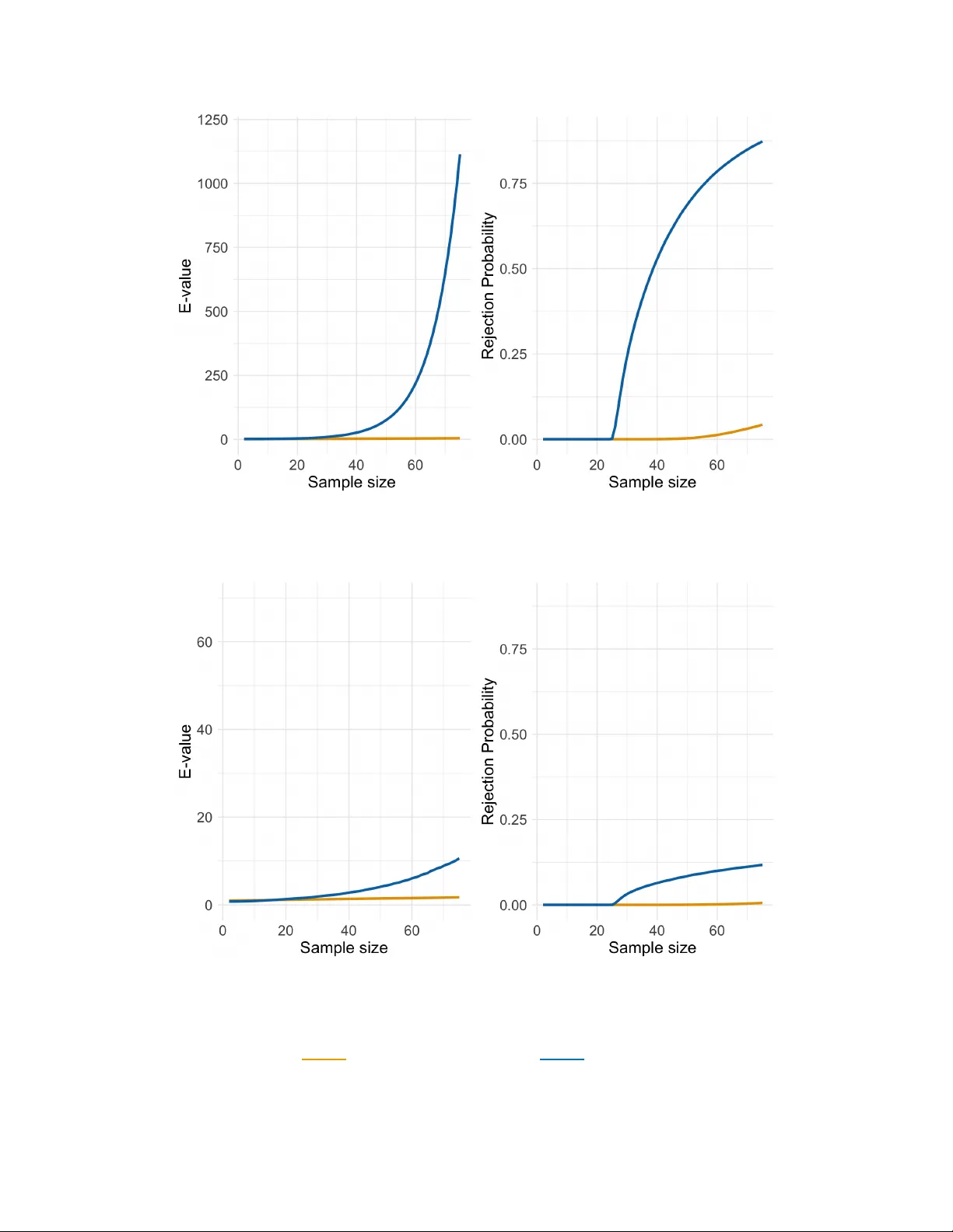
Equiv alence testing with data-dep enden t and p ost-ho c equiv alence margins ∗ Stan Ko obs † Nic k W. Koning ‡ Marc h 18, 2026 Abstract Equiv alence testing compares the h yp othesis that an eﬀect µ is large against the alternativ e that it is negligible. Here, ‘large’ is classically expressed as b eing larger than some ‘equiv alence m argin’ ∆. A longstanding problem is that this margin must b e sp eciﬁed but can rarely b e ob jectively justiﬁed in practice. W e la y the foundation for an alternative paradigm, arguing to instead rep ort a data-dep enden t margin b ∆ α that b ounds the true eﬀect µ with probability 1 − α . Our key argument is that b ∆ α is more useful than a test outcome at a ﬁxed margin ∆, as measured b y the guaran tees it oﬀers to decision mak ers. W e generalize this to a curve of margins α 7→ b ∆ α , uniformly v alid under the p ost-hoc selection of the margin. These ideas rely on e-v alues, which w e deriv e for mo dels that are strictly totally p ositiv e of order 3, nesting the classical z-test and t-test settings. ∗ W e are grateful to Isaiah Andrews, Josha Dekker, Peter Gr ¨ un wald, Jesse Hemerik, W outer Ko olen, Wietze Ko ops, Diego Martinez-T ab oada, Sam v an Meer, Iosif Pinelis, Aadity a Ramdas and participan ts at the CWI E-readers group and the 13th Econometric Internal PhD Conference at Erasmus Universit y Rotterdam for their insightful commen ts. † Econometric Institute, Erasm us Univ ersity Rotterdam. Email: k o obs@ese.eur.nl . ‡ Econometric Institute, Erasm us Univ ersity Rotterdam. Email: n.w.k oning@ese.eur.nl . 1 1 In tro duction Equiv alence assessmen t concerns the problem of establishing whether an eﬀect size µ ≥ 0 (or | µ | ) is suﬃcien tly small to b e deemed practically negligible. This problem arises across man y scien tiﬁc disciplines, including clinical trials and bio equiv alence assessmen t ( Sc huirmann , 1987 ; Berger and H su , 1996 ), psychology ( Lakens et al. , 2018 ), political science ( Hartman and Hidalgo , 2018 ), economics ( Dette and Sc h umann , 2024 ), and ecological sciences ( Robinson and F roese , 2004 ). Equiv alence assessment is almost univ ersally cast in to a hypothesis testing problem. Here, the analyst tests the n ull hypothesis H ∆ 0 : µ ≥ ∆ that the eﬀect µ is larger than some sp eciﬁed margin ∆, against the alternative H ∆ 1 : µ < ∆ that it is smaller. By sp ecifying ∆ to b e suﬃcien tly small so that eﬀect sizes µ < ∆ can b e viewed as (practically) equiv alen t to zero, this results in the level α > 0 T yp e-I error guarantee Pr(falsely claim equiv alence) ≡ Pr(falsely reject µ ≥ ∆) ≤ α. (1) A longstanding problem with this approac h is that the equiv alence margin ∆ is often diﬃcult to justify in practice. A t the same time, the formal Type-I error guaran tee ( 1 ) is inheren tly tied to the choice of ∆ through the null hypothesis H 0 : µ ≥ ∆: it only certiﬁes a claim of equiv alence r elative to the sp e ciﬁe d mar gin ∆. This creates an awkw ard tension: to obtain a formal guarantee one must commit to a margin ∆ that may b e hard to defend. This tension in vites a natural question: if the margin ∆ is hard to meaningfully sp ecify , is the Type-I error guaran tee ( 1 ) relativ e to such a margin ∆ actually what we w an t? That is, should equiv alence assessmen t even b e cast in to a testing problem? 1.1 Rep orting data-dep enden t equiv alence margins The main p oin t of this pap er is that equiv alence assessment should not b e cast into a testing problem. As a starting p oin t, we instead suggest reporting a data-dep endent e quivalenc e 2 mar gin b ∆ α that satisﬁes the guarantee Pr( µ < b ∆ α ) ≥ 1 − α, (2) for a data-indep endent α > 0. In w ords, b ∆ α ma y b e viewed as a statistically certiﬁed upp er b ound on µ , or as an upp er conﬁdence limit of a lev el 1 − α conﬁdence set [0 , b ∆ α ) for µ . T o motiv ate rep orting b ∆ α , w e argue that it is mor e useful than a test outcome, as measured by the guarantees it oﬀers to decision mak ers. In particular, suppose that the analyst hands b ∆ α to a decision maker facing a decision d ∈ D under a loss function L µ that is non-decreasing in the unkno wn parameter µ . Then, we show that the decision maker can use b ∆ α to translate the guarantee ( 2 ) in to the loss b ound Pr  L µ ( b d ) ≤ L b ∆ α ( b d )  ≥ 1 − α, (3) for every data-dep endent de cision b d . Within this framew ork, we ﬁnd that rep orting a ﬁxed-∆ test outcome is appropriate if the decision maker faces a loss L µ that dep ends only on whether µ < ∆ or µ ≥ ∆. How ever, the fact that ∆ is hard to sp ecify in practice suggests that practical decisions rarely hinge on a single ﬁxed ∆. As a consequence, w e argue that a ﬁxed-∆ test is generally not the appropriate metho dology for equiv alence assessment. W e formalize this discussion in Section 3 and Section 4 . There, w e show that a data- dep enden t margin b ∆ α is c haracterized by a sp eciﬁc c ol le ction of tests. Moreov er, w e formally deriv e the loss b ound ( 3 ). Loss b ounds such as ( 3 ) were recently studied by Andrews and Chen ( 2025 ) for classical conﬁdence sets and by Kiy ani et al. ( 2025 ) for conformal prediction. 1.2 Cho osing the equiv alence margin p ost-ho c W e distinguish the use of a data-dep endent margin b ∆ α from the p ost-ho c selection of the margin. T o explain this, note that it may b e tempting to compute an entire e quivalenc e curve α 7→ b ∆ α of data-dep enden t equiv alence margins and bro wse the curve to select the 3 desired certiﬁcate, p ost-ho c. Unfortunately , this would break the guarantee ( 2 ), since this mak es α data-dep enden t and ( 2 ) only holds for data-indep endent c hoices of α . T o resolv e this, w e consider recen t inno v ations in the data-dep enden t and p ost-ho c selection of α ( Gr ¨ un w ald , 2024 ; Koning , 2023 ). Using the approac h of Koning ( 2023 ), w e show ho w to obtain a uniformly valid equiv alence curv e α 7→ b ∆ α that satisﬁes E e α " Pr( µ ≥ b ∆ e α | e α ) e α # ≤ 1 , (4) for every data-dep endent level e α . This guaran tee ma y be in terpreted as rewriting ( 2 ) as Pr( µ ≥ b ∆ α ) /α ≤ 1 and upgrading from data-indep endent α to ‘in exp ectation ov er every data-dep enden t e α ’ ( not conditionally on e α = α ). As ( 4 ) holds for arbitrarily data-dep enden t levels e α , w e may truly browse the en tire equiv alence curve α 7→ b ∆ α and select the desired equiv alence margin b ∆ e α , p ost-ho c. W e displa y such a p ost-hoc v alid equiv alence curve in the left panel of Figure 1 . There, w e also sho w a data-dep endent margin b ∆ α at the ﬁxed lev el α = 0 . 05, whic h may b e viewed as a sp ecial uniformly v alid equiv alence curv e for which b ∆ e α = ∞ for e α < 0 . 05 and b ∆ e α = b ∆ α for e α ≥ α . W e see that the ﬁxed- α margin is tailored to α = 0 . 05 while the smo oth equiv alence curv e provides a balanced range of margins. W e formalize this discussion in Section 3.4 . Moreo ver, in Section 4 w e use ( 4 ) to generalize the loss b ound ( 3 ) to p ost-hoc loss b ounds, pro viding m uch more ﬂexibility to decision mak ers, inspired b y recent w ork of Koning and v an Meer ( 2025 ) and Gr ¨ unw ald ( 2023 ). 1.3 Connection to e-v alues and merging Under the ho o d, the data-dep enden t margin b ∆ α is deriv ed by inv erting a particular curv e of classical equiv alence tests ∆ 7→ ϕ ∆ . T o obtain uniformly v alid equiv alence curves α 7→ b ∆ α , w e generalize test in v ersion to inv erting a curv e of e-values ∆ 7→ ε ∆ for equiv alence. The e-v alue is a recen tly introduced measure of evidence, and ma y b e view ed as a con tin uous generalization of a classical hypothesis test ( Ho w ard et al. , 2021 ; Shafer , 2021 ; V o vk and 4 Figure 1: The left panel shows t w o uniformly v alid equiv alence curv es α 7→ b ∆ α , where the dashed line corresp onds to a ﬁxed- α data-dep endent margin. The righ t panel re-expresses these as curv es of e-v alues ∆ 7→ ε ∆ . W ang , 2021 ; Ramdas et al. , 2023 ; Gr ¨ un wald et al. , 2024 ; Koning , 2024 ; Ramdas and W ang , 2024 ). W e illustrate this e-v alue inv ersion in Figure 1 , where the righ t panel expresses the curv es in the left panel as curv es of e-v alues ∆ 7→ ε ∆ . There, the dashed line corresp onds to a curve of tests ∆ 7→ ϕ ∆ , which are { 0 , 1 /α } -v alued e-v alues. The curve ∆ 7→ ϕ ∆ switc hes from 0 to 1 /α at b ∆ α . A remark able consequence is that we can easily merge equiv alence curves α 7→ b ∆ α across studies (under indep endence) and across sp eciﬁcations (under arbitrary dep endence) b y translating them in to their curv e of e-v alues ∆ 7→ ε ∆ . Indeed, the pro duct of t wo indep endent curv es of e-v alues ∆ 7→ ε 1 ∆ × ε 2 ∆ is also a v alid curve of e-v alues. Moreo v er, the weigh ted a v erage of t wo arbitr arily dep endent curv es of e-v alues ∆ 7→ w ε 1 ∆ + (1 − w ) ε 2 ∆ , w ∈ [0 , 1], remains a v alid curv e of e-v alues. W e formally treat these merging prop erties in Section 3.5 . 1.4 T ec hnical con tributions Using the bridge b et w een equiv alence curv es and e-v alues, w e derive goo d equiv alence curv es b y deriving optimal e-v alues for equiv alence assessment. This constitutes our main technical con tribution. F or the optimalit y , w e restrict ourselv es to mo dels that are strictly totally p ositive of 5 order 3 (STP 3 ), whic h nests exp onen tial families, the z -test, t -test and more. Under this assumption, we show that the log-utility-optimal e-v alue ( Gr ¨ un w ald et al. , 2024 ; Larsson et al. , 2025 ) has a closed-form b oundary-mixture likelihoo d ratio. W e reco ver a similar structure when generalizing to general utility optimal e-v alues, whic h nests classically p o wer- optimal tests ( Lehmann , 1959 ; Romano , 2005 ) for the “Neyman–Pearson utility function” U α ( x ) = x ∧ 1 /α ( Koning , 2024 ). W e also in tro duce the TOST-E : the e-v alue generalization of the classical Tw o One- Sided T ests pro cedure ( Sc h uirmann , 1981 ). W e show it is v alid under the w eaker monotone lik eliho o d ratio condition (STP 2 ). W e also consider a (generalized) Universal Inference v arian t ( W asserman et al. , 2020 ), which is v alid under no assumptions. W e apply this theory to the z -test and t -test in Section 7 . The optimalit y is formally deriv ed in Section 5 , and the TOST-E and Univ ersal Inference v arian ts in Section 6 . Finally , in Section 8 , we dev elop anytime-v alid sequential extensions of these constructions. 1.5 Relationship to literature W e provide a short timeline of ho w equiv alence assessment w as originally cast into a testing problem. Moreo v er, we relate our work to several pap ers that caution against rep orting a data-dep enden t margin b ∆ α , and presen t our coun terargumen ts. T o the b est of our knowledge, testing equiv alence with a ﬁxed ∆ was ﬁrst considered in Chapter 3.7 of Lehmann ( 1959 ). The general problem of assessing equiv alence was studied b y W estlak e ( 1976 ; 1979 ) who eﬀectively prop osed rep orting b ∆ α . In an attempt to prop ose a ‘formal’ metho dology , Dunnett and Gent ( 1977 ) and Blac kwelder ( 1982 ) cast this into the ﬁxed-∆ testing framework of Lehmann ( 1959 ). This ﬁxed-∆ framew ork was subsequently consolidated b y regulatory b o dies for clinical trials, outlining that ∆ should b e presp eciﬁed in a transparen t and conserv ative manner, based on “[...] b oth statistical reasoning and clinical judgemen t [...]” ( In ternational Conference on Harmonisation , 1998 ; 2000 ). A large b o dy of literature has subsequen tly fo cused on ho w one should motiv ate ∆ ( Wiens , 2002 ; Lange 6 and F reitag , 2005 ; Fitzgerald , 2025 ). Based on recent draft regulations of the Europ ean Medicines Agency ( 2025 ), the ﬁxed-∆ testing approach remains the standard to this da y . F ollo wing the original prop osal b y W estlake ( 1976 ), sev eral other pap ers hav e discussed rep orting a data-dep enden t margin b ∆ α , based on inv erting v arious tests. In particular, Hauc k and Anderson ( 1986 ) propose o vercoming the presp eciﬁcation of ∆, b y plotting a (not uniformly v alid) equiv alence curv e α 7→ b ∆ α , as a “useful wa y to present [...] the degree of certaint y regarding p oten tial diﬀerences”. Moreov er, b oth Seaman and Serlin ( 1998 ) and Meyners ( 2007 ) propose rep orting a v ariant of b ∆ α based on in verting the TOST of Sc h uirmann ( 1981 ). W e stress that these w orks explicitly only view b ∆ α as an informal, exploratory , descriptive or diagnostic to ol, and not as a replacemen t of the ﬁxed-∆ testing metho dology . Key argumen ts against viewing b ∆ α as a serious alternativ e to the ﬁxed-∆ approac h are presen ted in Ng ( 2003 ) and Campb ell and Gustafson ( 2021 ). Both argumen ts rely on casting equiv alence assessment bac k into a binary testing problem, sho wing that no meaningful Type- I error con trol can b e achiev ed for the data-dep endent hypothesis H b ∆ α . Indeed, Campb ell and Gustafson ( 2021 ) observe that H b ∆ α is rejected b y construction, leading to the conclusion that rep orting b ∆ α “[...] lacks the formalism of equiv alence testing [...]”. Ng ( 2003 ) similarly argues that the data-dep endent h yp othesis H b ∆ α w ould b e rejected in an identical rep eated exp erimen t with probabilit y 1/2, concluding that rep orting b ∆ α is “[...] exploratory and [...] unacceptable for conﬁrmatory testing [...]”. Our main coun terargument bypasses this discussion: we b eliev e it is not relev ant whether w e can obtain a Type-I error control on rejecting H b ∆ α . Instead, we b eliev e that one should simply compare statistical pro cedures by ho w useful they are in subsequent decision making. There, w e argue that the guarantee ( 2 ) on b ∆ α is more useful and no less ‘formal’ than a T yp e-I error guaran tee for a ﬁxed ∆. 7 2 Bac kground: from tests to e-v alues W e denote a sample space b y X , whic h w e equip with a mo del P : a collection of probabilities on X . A h yp othesis H ⊆ P is a subset of our mo del. The inten tion of hypothesis testing is to obtain evidence against a h yp othesis H . Without loss of generality , w e follow Koning ( 2024 ) in deﬁning a h yp othesis test ϕ α as a { 0 , 1 /α } -v alued map. Here, ϕ α = 0 is in terpreted as a non-rejection and ϕ α = 1 /α as a rejection at level α > 0. This may b e interpreted as emitting either no evidence (0) or a particular amount of evidence (1 /α ) against a hypothesis. Deﬁnition 1 (T est) . A level- α test is a me asur able map ϕ α : X → { 0 , 1 /α } . A test ϕ α is valid for hyp othesis H if E P [ ϕ α ] ≡ P ( ϕ α = 1 /α ) /α ≤ 1 , for ev ery P ∈ H . The e-value can b e view ed as a ‘multi-signiﬁcance level’ generalization of a test. Indeed, the e-v alue extends the binary co domain { 0 , 1 /α } of a test to the richer { 0 , 1 /α 1 , 1 /α 2 , . . . } , α 1 , α 2 , · · · > 0, or ev en [0 , ∞ ]. This means an e-v alue ma y return v arious amoun ts of evidence against the h yp othesis. In particular, the realization of an e-v alue ε may b e interpreted as a rejection at lev el 1 /ε under a generalized T yp e-I error guaran tee ( Koning , 2023 ). Deﬁnition 2 (E-v alue) . A n e-value is a me asur able map ε : X → [0 , ∞ ] . An e-value ε is valid for hyp othesis H if E P [ ε ] ≤ 1 , for ev ery P ∈ H . 3 Equiv alence assessmen t In this section, w e deriv e the equiv alence betw een data-dependent margins b ∆ α and particular curv es of tests ∆ 7→ ϕ ∆ , and generalize this to uniformly v alid equiv alence curves α 7→ b ∆ α and particular curv es of e-v alues ∆ 7→ ε ∆ . F or now, w e fo cus on a single margin b ∆ α instead of the pair of margins ( b ∆ − α , b ∆ + α ) typical in equiv alence testing, b ecause suc h a pair in tro duces considerable notational o verhead without adding conceptual insight. The single-margin setting is also kno wn in the literature as assessing ‘non-inferiority’ ( W ellek , 2010 ). W e co v er margin pairs in Section 3.6 . 8 3.1 Mo del and h yp otheses T o formally set up assessing equiv alence, w e consider a mo del ( P µ ) µ ≥ 0 indexed by a parameter µ . W e use µ ∗ to denote the parameter asso ciated to the ‘true’ data generating pro cess P µ ∗ . W e consider a collection of hypotheses ( H ∆ 0 ) ∆ ≥ 0 of the form H ∆ 0 = { P µ : µ ≥ ∆ } . Here, the h yp othesis H ∆ 0 ma y b e in terpreted as the statemen t that µ ∗ is at least ∆. By the structure of the problem, the index ∆ ∗ of the smallest true h yp othesis H ∆ ∗ 0 coincides with µ ∗ , since ∆ ∗ = inf { ∆ ∈ [0 , ∞ ) : µ ∗ ≤ ∆ } = µ ∗ . T o av oid causing confusion b y frequen tly switching back and forth b et ween ∆ and µ , we use this identit y to formulate the problem as obtaining a b ound on ∆ ∗ . 3.2 Data-dep enden t margins In theory , we w ould desire a probabilistic data-dependent b ound b ∆ α on ∆ ∗ that is v alid under the smallest true hypothesis: sup µ ≥ ∆ ∗ P µ (∆ ∗ ≥ b ∆ α ) ≤ α . Ho w ever, as the true v alue ∆ ∗ is unkno wn, and w e do not wish to take a stance on its v alue, we ac hieve this b y requiring this inequality to hold for every margin ∆. This leads us to Deﬁnition 3 . Deﬁnition 3 (V alid data-dep enden t margin) . A mar gin b ∆ α is valid at level α > 0 if sup ∆ ≥ 0 P ∆ (∆ ≥ b ∆ α ) ≤ α . (5) Remark 1. The guar ante e ( 5 ) is e quivalent to sup ∆ ≥ 0 sup µ ≥ ∆ P µ (∆ ≥ b ∆ α ) ≤ α . Remark 2. The data-dep endent mar gin b ∆ α may b e interpr ete d as the upp er b ound of a c onﬁdenc e set [0 , b ∆ α ) for ∆ ∗ . 3.3 Data-dep enden t margins and test in version In Prop osition 1 , w e show that b ∆ α is uniquely c haracterized by a non-decreasing curv e ∆ 7→ ϕ α ∆ of equiv alence tests for H ∆ 0 . This means that b ∆ α and ∆ 7→ ϕ α ∆ can b e viewed as t w o diﬀeren t represen tations of the same information. Moreov er, it implies that to construct 9 b ∆ α , w e can reduce to the familiar task of constructing an equiv alence test ϕ α ∆ , for ev ery h yp othesis H ∆ 0 . The pro of of Prop osition 1 is found in App endix A.1 , which also carefully handles the measurabilit y of b ∆ α . The precise corresp ondence betw een the data-dep enden t margin and curv e of tests is that the margin b ∆ α induces the tests ϕ α ∆ = I { ∆ ≥ b ∆ α } /α . Conv ersely , the data-dep enden t margin can b e retrieved by inv erting a curve of tests ∆ 7→ ϕ α ∆ through b ∆ α = inf { ∆ : ϕ α ∆ = 1 /α } . Prop osition 1. A data-dep endent mar gin b ∆ α c orr esp onds to a non-de cr e asing right-c ontinuous curve ∆ 7→ ϕ α ∆ of tests. b ∆ α is valid if and only if ϕ α ∆ is valid for H ∆ 0 for every ∆ ≥ 0 . Remark 3 (Non-decreasing in ∆) . Inverting a c ol le ction of tests that is not non-de cr e asing in ∆ may r esult in a c onﬁdenc e set that is not an interval of the form [0 , b ∆ α ) . While ther e is nothing fundamental ly wr ong with such a c onﬁdenc e set for ∆ ∗ , it is har der to interpr et, b e c ause it assigns mor e evidenc e against smal ler values of ∆ (lar ger hyp otheses) than against lar ger values of ∆ (smal ler hyp otheses). In Se ction 5 , we ﬁnd that optimal tests ar e gener al ly non-de cr e asing in ∆ . Mor e over, we c an c onvert any family of tests into a non-de cr e asing family by taking its right-lower envelop e ϕ α ∆ ( x ) := inf ∆ ′ ≥ ∆ ϕ α ∆ ′ ( x ) . 3.4 Uniform v alidit y , p ost-ho c margins and e-v alue in v ersion W e no w generalize beyond tests to e-v alues to construct uniformly v alid equiv alence curves α 7→ b ∆ α . In particular, w e consider a non-decreasing collection ∆ 7→ ε ∆ of e-v alues ε ∆ v alid for H ∆ 0 . W e then generalize test inv ersion to e-v alue inv ersion by constructing a non- increasing equiv alence curv e through b ∆ α = inf { ∆ : ε ∆ ≥ 1 /α } . The k ey contribution here is that this do es not merely result in a curve of individual ly valid margins b ∆ α . Instead, the curve α 7→ b ∆ α is uniformly valid , as deﬁned in Deﬁnition 4 . This result is presented in Theorem 1 , whic h is prov en in App endix A.2 . 10 The consequence of uniform v alidity is that w e ma y in terpret the en tire equiv alence curv e α 7→ b ∆ α as a whole. F or example, it enables the p ost-ho c sele ction of the margin: w e ma y bro wse the curve α 7→ b ∆ α and select the data-dep enden t lev el e α that comes with the desired v alue of b ∆ e α . Deﬁnition 4. We say that the e quivalenc e curve α 7→ b ∆ α is uniformly valid if sup ∆ ≥ 0 E P ∆ e α " P ∆ (∆ ≥ b ∆ e α | e α ) e α # ≤ 1 , for every data-dep endent choic e of the level e α > 0 . Theorem 1. A non-incr e asing and right-c ontinuous e quivalenc e curve α 7→ b ∆ α c orr esp onds to a non-de cr e asing and right-c ontinuous c ol le ction of e-values ∆ 7→ ε ∆ . The e quivalenc e curve is uniformly valid if and only if every e-value ε ∆ is valid for H ∆ 0 . Remark 4. ∆ 7→ ε ∆ c an b e obtaine d fr om the e quivalenc e curve: ε ∆ = sup n 1 α : ∆ ≥ b ∆ α o . Remark 5. As e-values gener alize tests, the discussion her e is a (rich) gener alization of Se ction 3.3 . In p articular, ﬁxing the level α = a , a data-dep endent mar gin b ∆ a c orr esp onds to the e quivalenc e curve α 7→ e ∆ α for which e ∆ α = ∞ for α < a and e ∆ α = b ∆ a for α ≥ a . Remark 6 (Evidence non-decreasing in ∆) . R emark 3 extends to e-values. Inde e d, if ∆ 7→ ε ∆ wer e not non-de cr e asing, then we c ould have mor e evidenc e against lar ger hyp otheses than against the smal ler hyp otheses neste d within them. If ne c essary, we c an also take the right-lower envelop e to enfor c e this: ε ∆ ( x ) := inf ∆ ′ ≥ ∆ ε ∆ ′ ( x ) . 3.5 Merging equiv alence curv es Merging evidence is important in equiv alence assessment: evidence for the same problem may come from m ultiple indep enden t studies, or m ultiple analyses based on diﬀerent sp eciﬁcations ma y be p erformed on the same data. One of the attractiv e features of e-v alues is that they enable easy merging of evidence ( V o vk and W ang , 2021 ). Using the link b et w een curv es of e-v alues and equiv alence curves, we extend these merging op erations to equiv alence curves. 11 In particular, consider t w o non-decreasing curves of v alid e-v alues, ∆ 7→ ε j ∆ , j = 1 , 2. Their weigh ted av erage ∆ 7→ w ε 1 ∆ + (1 − w ) ε 2 ∆ is a curve of v alid e-v alues, w ∈ [0 , 1]. If b oth are independent, then their pro duct ∆ 7→ ε 1 ∆ ε 2 ∆ is a curve of v alid e-v alues. By Theorem 1 , in v erting this merged curv e of e-v alues pro duces a merged uniformly v alid equiv alence curve. In Prop osition 2 , w e show this merging can b e expressed in terms of equiv alence curves. Prop osition 2. L et α 7→ b ∆ 1 α and α 7→ b ∆ 2 α b e two uniformly valid e quivalenc e curves. Then, the fol lowing e quivalenc e curve is uniformly valid: b ∆ w α = inf α 1 ,α 2 > 0: w α 1 + 1 − w α 2 = 1 α max { b ∆ 1 α 1 , b ∆ 2 α 2 } . If the curves ar e indep endent, then the fol lowing curve is also uniformly valid: b ∆ × α = inf α 1 ,α 2 > 0: α 1 α 2 = α max { b ∆ 1 α 1 , b ∆ 2 α 2 } . 3.6 Tw o margins Up to this p oint, we hav e fo cused on a single margin to facilitate the presen tation of our ideas, expressed in terms of one-sided h yp otheses H ∆ 0 : µ ≥ ∆. W e no w turn to the tw o-sided v ersion of equiv alence testing, expressed by hypotheses of the form H (∆ − , ∆ + ) 0 : µ ≤ ∆ − or µ ≥ ∆ + , for a pair of margins ∆ − ≤ ∆ + , and a real-v alued parameter µ ∈ R . This reco vers the one-sided setting if we set ∆ − = −∞ , or ∆ − = 0 if µ ∈ R + . F or assessing equiv alence in this tw o-sided setting, w e may consider an e-v alue ε ∆ − , ∆ + for eac h hypothesis H (∆ − , ∆ + ) 0 , and so for each pair of margins (∆ − , ∆ + ). A resulting curve of e-v alues (∆ − , ∆ + ) 7→ ε ∆ − , ∆ + is then assumed to b e non-decreasing co ordinate-wise: in the partial order ≾ that is deﬁned by (∆ − 1 , ∆ + 1 ) ≾ (∆ − 2 , ∆ + 2 ) if and only if b oth ∆ − 1 ≥ ∆ − 2 and ∆ + 1 ≤ ∆ + 2 . That is, ε ∆ − 1 , ∆ + 1 ≤ ε ∆ − 2 , ∆ + 2 if (∆ − 1 , ∆ + 1 ) ≾ (∆ − 2 , ∆ + 2 ). 12 T o obtain the tw o-margin analogue of an equiv alence curve α 7→ b ∆ α , we can similarly in v ert a curve of e-v alues. Here, w e do not merely obtain a pair ( b ∆ − α , b ∆ + α ) of margins for eac h α . Instead, we obtain a collection of pairs for every α : b D α = inf { (∆ − , ∆ + ) : ε ∆ − , ∆ + ≥ 1 /α } , where the inﬁmum here is interpreted to pro duce the set of maximal low er b ounds in the partial order ≾ . 4 Evidence-certiﬁed decisions In this section, w e motiv ate our call to rep ort a data-dep endent margin b ∆ α , or a more general uniformly v alid curv e of margins α 7→ b ∆ α , instead of a classical ﬁxed-∆ equiv alence test outcome ϕ ∆ . F or this purp ose, we study the guaran tees pro vided b y these ob jects to decision makers. In particular, w e consider a decision maker who faces a decision d ∈ D based on a loss function L µ : D → [0 , ∞ ) that is non-decreasing and left-con tinuous in the (unknown) true v alue µ ∗ of µ , for ev ery decision d ∈ D . The decision maker receiv es information ab out µ ∗ in the form of a data-dep enden t margin b ∆ α , or equiv alence curv e α 7→ b ∆ α , to aid in the decision making pro cess. Example 1. The de cision maker may b e a r e gulator who ne e ds to make a de cision d on the r e c ommende d daily c onsumption of a c ertain fo o d item, b ase d on the unknown c onc entr ation µ ∗ of a p otential ly harmful substanc e in the fo o d item. Her e, the loss L µ may describ e the exp e cte d ne gative imp act on public he alth asso ciate d with e ach de cision if µ is the true c onc entr ation, wher e higher c onc entr ations r esult in a lar ger ne gative imp act. A test ϕ ∆ , data-dep endent mar gin b ∆ α or e quivalenc e curve α 7→ b ∆ α expr esses the information ab out µ ∗ that is available to the de cision maker. 13 4.1 Decisions based on a data-dep enden t margin In Theorem 2 , w e show how the v alidity ( 5 ) of a data-dep endent margin b ∆ α can b e passed on to a uniform loss b ound across data-dep enden t decisions. This b ound is expressed b y the loss function L b ∆ α at µ = b ∆ α . The interpretation of this result is that whatev er the true v alue µ ∗ is, the probabilit y that a decision b d yields a loss greater than L b ∆ α ( b d ) is small. Theorem 2 (Uniform loss b ound) . If b ∆ α is valid, then sup µ ≥ 0 P µ ( L µ ( b d ) > L b ∆ α ( b d )) ≤ α , for every data-dep endent de cision b d . Pr o of. As µ 7→ L µ ( d ) is non-decreasing for eac h d , we hav e L µ ( b d ) > L b ∆ α ( b d ) = ⇒ b ∆ α ≤ µ . V alidit y of b ∆ α then implies sup µ ≥ 0 P µ ( L µ ( b d ) > L b ∆ α ( b d )) ≤ sup µ ≥ 0 P µ ( µ ≥ b ∆ α ) ≤ α . This loss b ound is inspired by recent w ork on certifying decisions b y Andrews and Chen ( 2025 ). They fo cus on the decision that attains the tightest b ound: the minimax decision b d MM α ∈ arg min d ∈D sup µ< b ∆ α L µ ( d ) = arg min d ∈D L b ∆ α ( d ), assuming it exists. Suc h a minimax decision is also known as an as-if decision, b ecause the decision is made ‘as-if ’ µ ∗ < b ∆ α ( Manski , 2021 ). Our Theorem 2 is more than an application of Andrews and Chen ( 2025 ) to equiv alence assessmen t. The inno v ation here is that our result holds uniformly across all data-dep endent decisions, whereas Andrews and Chen ( 2025 ) only consider the minimax decision. This is imp ortan t, b ecause even though the minimax decision attains the tightest b ound, decision mak ers ma y opt for a diﬀerent decision for external reasons. Our result still pro vides a loss b ound on suc h decisions. Moreov er, it a v oids the technical problem of requiring the existence of a minimax decision. 4.2 When is a classical equiv alence test suﬃcien t? The loss b ound pro vided in Theorem 2 pro vides a strong motiv ation for rep orting a data- dep enden t margin b ∆ α . At the same time, this analysis raises a natural question: for what kind of loss function w ould the outcome of a classical ﬁxed-∆ equiv alence test b e suﬃcient? 14 In this section, w e show that a classical equiv alence test ϕ ∆ is suﬃcien t if the loss function hinges on a ﬁxed ∆. Consider a loss function L µ for whic h the loss L µ ( d ) of every decision only dep ends on whether µ ≤ ∆. That is, for ev ery d ∈ D there exist v alues ℓ − ( d ) ≤ ℓ + ( d ) such that L µ ( d ) = ℓ − ( d ) I { µ ≤ ∆ } + ℓ + ( d ) I { µ > ∆ } . This means that the b ound L b ∆ α ( b d ) on the loss L µ ( b d ) in Theorem 2 only dep ends on the data through the outcome of the test ϕ ∆ = I { b ∆ α ≤ ∆ } /α . Indeed, substituting this loss into Theorem 2 yields the loss b ound sup µ ≥ 0 P µ  L µ ( b d ) > ℓ − ( b d ) I { b ∆ α ≤ ∆ } + ℓ + ( b d ) I { b ∆ α > ∆ }  ≤ α. As a result, the outcome of the test ϕ ∆ is the relev ant information for the decision mak er. T o see this more directly , w e can sho w that the minimax decision only hinges on the outcome of ϕ ∆ . Indeed, for this loss function we hav e that the optimal decision d ∗ ( µ ) ∈ arg min d ∈D L µ ( d ) only dep ends on whether µ ≤ ∆: d ∗ ( µ ) = arg min d ∈D ℓ − ( d ) =: d − if µ ≤ ∆ and d ∗ ( µ ) = arg min d ∈D ℓ + ( d ) =: d + if µ > ∆. Substituting b ∆ α in for µ yields that the minimax decision equals b d MM α = d − if ϕ ∆ rejects and b d MM α = d + , otherwise. This analysis sho ws the outcome of a single ﬁxed-∆ equiv alence test ϕ ∆ is relev ant if the loss L µ hinges on this v alue of ∆. At the same time, the fact that ∆ is hard to sp ecify in practice suggests that loss functions rarely hinge on a single v alue of ∆ in practice. Indeed, if practical loss functions w ould often hinge on a single ∆, then we b elieve practitioners w ould not struggle as m uc h to pick ∆. This supp orts our conclusion that a single test outcome ϕ ∆ is not the right statistical ob ject to rep ort, and that rep orting b ∆ α is more appropriate. 4.3 Decisions based on equiv alence curv es In Theorem 3 , we generalize Theorem 2 to uniformly v alid equiv alence curv es α 7→ b ∆ α . In this setting, the loss b ound is now represen ted b y a sp ectrum of loss functions α 7→ L b ∆ α that 15 is uniformly v alid in the conﬁdence certiﬁcate α . Theorem 3. If α 7→ b ∆ α is uniformly valid, then sup µ ≥ 0 E P µ e α " P µ ( L µ ( b d ) > L b ∆ e α ( b d ) | e α ) e α # ≤ 1 , for every data-dep endent de cision b d and data-dep endent level e α . There are v arious w ays to use this loss sp ectrum: • Giv en an arbitrary data-dep endent decision b d , it provides a sp ectrum α 7→ L b ∆ α ( b d ) of loss b ounds on L µ ( b d ), each coupled with a diﬀeren t conﬁdence lev el α . • Giv en a post-ho c c hoice of the margin ∆, we can retrieve the corresp onding data- dep enden t conﬁdence lev el e α = inf { α : ∆ ≥ b ∆ α } from the equiv alence curve α 7→ b ∆ α to obtain the loss function d 7→ L b ∆ e α ( d ). • Giv en a p ost-ho c choice of the conﬁdence lev el e α , we can retrieve the corresp onding margin b ∆ e α and obtain the matching loss function d 7→ L b ∆ e α ( d ). One concrete idea is to present the decision mak er with an entire sp ectrum of minimax decisions and their asso ciated loss b ounds: α 7→ ( b d MM α , L b ∆ α ( b d MM α )), where b d MM α ∈ arg min d ∈D L b ∆ α ( d ). A decision maker may then bro wse such decisions and select the decision with the desired loss b ound ( Koning and v an Meer , 2025 ). Remark 7. An alternative ide a pr op ose d by Gr ¨ unwald ( 2023 ) is to de-emphasize implausible values of ∆ by weighting the L ∆ by the amount of evidenc e ε ∆ against ∆ . This le ads to weighte d minimax de cisions arg min d ∈D sup ∆ ≥ 0 L ∆ ( d ) /ε ∆ , for non-ne gative loss functions L ∆ . 5 Optimal e-v alues for equiv alence under STP 3 In Section 3 , w e established uniform v alidity of equiv alence curv es obtained by in v erting e-v alues. How ever, v alidity alone is not suﬃcien t to guarantee that a curv e is informativ e. 16 Indeed, a curv e for whic h b ∆ α = ∞ for every α is also uniformly v alid, but completely uninformativ e. Because these curves are obtained b y inv erting a curv e of e-v alues ∆ 7→ ε ∆ , the remainder of this pap er fo cuses on studying go od e-v alues. In this section, we switc h to the tw o-sided equiv alence setting, cov ering hypotheses of the form H (∆ − , ∆ + ) 0 : µ ≤ ∆ − or µ ≥ ∆ + as discussed in Section 3.6 . W e mak e this switc h because the optimalit y results for the tw o-sided setting are conceptually ric her and technically more demanding than the one-sided claims. 1 5.1 Setup and STP 3 W e consider a single-parameter mo del ( P µ ) µ ∈M dominated by a σ -ﬁnite measure ν , where M ⊆ R . W e consider a sample space X ⊆ R , which ma y b e interpreted as the sample space of a (suﬃcien t) statistic. W e denote the densit y of P µ with resp ect to ν b y p µ = dP µ /dν . Fix ∆ − < ∆ + with ∆ − , ∆ + ∈ M . W e consider the h yp otheses, H (∆ − , ∆ + ) 0 = { P µ : µ ≤ ∆ − or µ ≥ ∆ + } , H (∆ − , ∆ + ) 1 = { P µ : ∆ − < µ < ∆ + } , assuming that b oth are non-empty . W e make one structural assumption: w e assume strict total p ositivit y of order 3 (STP 3 ) of the k ernel ( µ, x ) 7→ p µ ( x ) ( Karlin , 1968 ). The formal deﬁnition of STP 3 is quite tec hnical, and so deferred to App endix B . STP 3 is satisﬁed, for example, by exp onen tial families. Remark 8 (STP 3 , STP 2 and MLR) . STP 3 may b e interpr ete d as a str engthene d version of the Monotone Likeliho o d R atio assumption (MLR), which c oincides with STP 2 . Wher e MLR c ontr ols p airwise likeliho o d-r atio monotonicity, STP 3 additional ly c ontr ols a triplewise or dering. This additional structur e is pr e cisely what delivers the variation-diminishing pr op erties use d b elow ( Br own et al. , 1981 ). 1 The one-sided results can b e viewed as a limiting sp ecial case, obtained b y taking ∆ − → −∞ which leads to setting c = 0 in Theorem 4 , only requiring STP 2 . 17 5.2 Neyman-P earson optimalit y W e start b y brieﬂy co vering the familiar Neyman-P earson optimality framew ork. Under STP 3 a uniformly most p ow erful (UMP) test is kno wn to exist. Its critical region is determined by a lik eliho o d ratio against a mixture of the tw o b oundary densities ( Lehmann , 1959 ; Kallen b erg and Janssen , 1984 ). Concretely , for an y P µ ∈ H (∆ − , ∆ + ) 1 , the classical lev el- α UMP test can b e written as a sp ecial e-v alue ε α ( x ) = 1 α I { Λ c ( x ) > k α } + η α ( x ) α I { Λ c ( x ) = k α } , Λ c ( x ) := p µ ( x ) c p ∆ − ( x ) + (1 − c ) p ∆ + ( x ) , where c ∈ [0 , 1], k α > 0, and η α : X → [0 , 1] are c hosen to satisfy the boundary size equalities E P ∆ − [ ε α ( X )] = E P ∆ + [ ε α ( X )] = 1. Here, the case that Λ c ( x ) = k α is classically interpreted as an instruction to reject with probabilit y η α ( x ) using external randomization. Ho w ever, w e follo w Koning ( 2024 ) in recommending to instead rep ort ε α ( x ) directly as evidence. 5.3 Utilit y-optimal e-v alues The classical Neyman-Pearson framew ork can b e view ed as a sp ecial case of a more general optimal e-v alue setting. In particular, a natural goal is to select an e-v alue that maximizes the exp ected utilit y E P µ [ U ( ε )] under some alternativ e P µ ∈ H (∆ − , ∆ + ) 1 for some utility function U : [0 , ∞ ] → [ −∞ , ∞ ]. Indeed, this can be sho wn to reco ver the Neyman-P earson framew ork for the ‘Neyman-P earson utility function’ U α ( e ) = min { e, 1 /α } ( Koning , 2024 ). Bey ond the Neyman-Pearson utility function, one can generally not exp ect an e-v alue to b e expected-utility optimal ov er a comp osite hypothesis H (∆ − , ∆ + ) 1 . W e therefore instead maximize the exp ected utilit y E Q [ U ( ε )] under a mixture alternative Q = R P µ dw ( µ ), where w is a mixture o v er H (∆ − , ∆ + ) 1 . In practice, w may b e chosen as a Dirac measure on some relev an t p oint (e.g. w = δ 0 if µ = 0 is a relev ant alternative), or as some kind of uniform distribution ov er the interv al [∆ − , ∆ + ]. Let E denote the class of v alid e-v alues for H (∆ − , ∆ + ) 0 . Assume that U : [0 , ∞ ] → [ −∞ , ∞ ] 18 is increasing, strictly conca ve and con tin uously diﬀerentiable on (0 , ∞ ). Moreov er, assume that its deriv ative U ′ satisﬁes lim x →∞ U ′ ( x ) = 0. T o ensure that the optimizer exists without restrictions on the distributions, we assume x 7→ xU ′ ( x ) is b ounded. Theorem 4 presen ts our main optimalit y result. As in the classical Neyman-Pearson case, these utility-optimal e-v alues also in v olv e a b oundary-mixture likelihoo d ratio. Theorem 4. Assume { p µ : µ ∈ M} is STP 3 , and let q b e the density of the mixtur e alternative Q with r esp e ct to ν . F or c ∈ (0 , 1) and λ > 0 , deﬁne ε c,λ ( x ) := ( U ′ ) − 1  λ c p ∆ − ( x ) + (1 − c ) p ∆ + ( x ) q ( x )  . Then ther e exists ( c ∗ , λ ∗ ) ∈ (0 , 1) × (0 , ∞ ) such that ε c ∗ ,λ ∗ is the U -optimal e-variable, i.e. ε c ∗ ,λ ∗ ∈ arg max ε ∈E E Q [ U ( ε )] . Corollary 1 cov ers the p opular log-utilit y ( Gr ¨ un wald et al. , 2024 ; Larsson et al. , 2025 ). Corollary 1 (Log-optimal e-v alue) . Under U ( e ) = log e , The or em 4 yields ε c ∗ ( x ) = q ( x ) c ∗ p ∆ − ( x ) + (1 − c ∗ ) p ∆ + ( x ) . 5.4 Commen ts on the pro of of Theorem 4 The pro of of Theorem 4 rests on tw o STP 3 -based ingredients. The ﬁrst is a calibration result: it determines ( c, λ ) by ensuring that ε c,λ has exp ectation exactly 1 at b oth b oundary p oints. The second is a shap e result: it ensures that x 7→ ε c,λ ( x ) has at most one lo cal extremum, whic h is what allows b oundary calibration to extend to the en tire composite n ull. Prop osition 3. Ther e exists ( c ∗ , λ ∗ ) ∈ (0 , 1) × (0 , ∞ ) such that E ∆ − [ ε c ∗ ,λ ∗ ( X )] = 1 and E ∆ + [ ε c ∗ ,λ ∗ ( X )] = 1 . Prop osition 4. F or every c ∈ (0 , 1) and λ > 0 , x 7→ ε c,λ ( x ) has at most one lo c al extr emum. 19 Remark 9 (W eakening to STP 2 ) . The STP 3 assumption in The or em 4 c annot, in gener al, b e we akene d to STP 2 (MLR). In p articular, ther e ar e STP 2 families for which the likeliho o d r atio ε c with c chosen to satisfy the b oundary size c onditions is not a valid e-variable for the ful l c omp osite nul l. A c ounter example is given in App endix B : STP 2 holds but STP 3 fails, and the r esulting c andidate violates e-value validity at another nul l p ar ameter value. 6 TOST and Univ ersal Inference 6.1 The TOST-E P erhaps the most widely used test for equiv alence testing is the Tw o One-Sided T ests (TOST) pro cedure ( Sch uirmann , 1981 ; 1987 ). As the name suggests, the idea is to test b oth H L 0 : µ ≤ ∆ − and H R 0 : µ ≥ ∆ + at level α , and reject the equiv alence null H (∆ − , ∆ + ) 0 if b oth are rejected. Generalizing from tests to e-v alues, w e introduce the TOST-E pro cedure based on t wo one-sided e-v alues ε L and ε R for H L 0 and H R 0 . Since e-v alues pro duce a con tin uous amount of evidence, the natural generalization is to tak e their minimum: ε TOST ( x ) := min { ε L ( x ) , ε R ( x ) } . As ε L and ε R are v alid for H L 0 and H R 0 , this minimum is indeed v alid for their union H (∆ − , ∆ + ) 0 . In the exp ected-utilit y framew ork, a natural choice for the one-sided e-v alues is ε L ( x ) := ( U ′ ) − 1 ( p ∆ − ( x ) /q ( x )) and ε R ( x ) := ( U ′ ) − 1 ( p ∆ + ( x ) /q ( x )). Under STP 2 (MLR), these are v alid for H L 0 and H R 0 , so that their combined TOST-E is v alid under STP 2 . Remark 10 (Comparison log-optimal and TOST-E) . T aking U = log , the TOST-E c an b e written as ε TOST ( x ) = q ( x ) / max { p ∆ − ( x ) , p ∆ + ( x ) } . Comp aring this to the lo g-optimal e-variable ε lo g ( x ) = q ( x ) / ( c ∗ p ∆ − + (1 − c ∗ ) p ∆ + ) , we ﬁnd ε lo g ( x ) ≥ ε TOST ( x ) for every x ∈ X , sinc e max { p ∆ − ( x ) , p ∆ + ( x ) } ≥ c ∗ p ∆ − + (1 − c ∗ ) p ∆ + . As a r esult, the lo g-optimal e-value dominates the TOST-E, at the c ost of r e quiring STP 3 over STP 2 . 20 6.2 Univ ersal inference If ( P µ ) µ ∈M is not STP 2 , an option is to rely on (a generalization of ) Universal Inference ( W asserman et al. , 2020 ), which is v alid without assumptions on the mo del ( P µ ) µ ∈M . Instead of taking the minimum of tw o one-sided e-v alues for the b oundary hypotheses H L 0 : µ ≤ ∆ − and H R 0 : µ ≥ ∆ + , the (generalized) Universal Inference approac h tak es the essen tial inﬁm um 2 essinf µ ∈M 0 ε µ o v er a collection of e-v alues ( ε µ ) µ ∈M 0 where ε µ is v alid for the h yp othesis { P µ } and M 0 = { µ : P µ ∈ H ∆ − , ∆ + 0 } . While this approac h may seem o verly conserv ativ e, every v alid e-v alue can b e interpreted as a sp ecial case of generalized Universal Inference (see e.g. Prop osition 3 in Koning and v an Meer ( 2026 )). Remark 11 (Comparison TOST-E and UI) . The name Universal Infer enc e is usual ly r eserve d for an inﬁmum over lo g-optimal / likeliho o d r atio e-values ε µ = q ( x ) /p µ ( x ) . The r esulting e-value ε UI = essinf µ ∈M 0 q ( x ) /p µ ( x ) = q ( x ) / esssup µ ∈M 0 p µ ( x ) is dominate d by its TOST-E c ounterp art q ( x ) / max { p ∆ − , p ∆ + } , sinc e esssup µ ∈M 0 p µ ( x ) ≥ max { p ∆ − , p ∆ + } . 7 Examples: z -test & t -test 7.1 z -test Let X 1 , . . . , X n iid ∼ N ( µ, σ 2 ) with kno wn v ariance σ 2 . W e ﬁx the margins ∆ − < ∆ + and consider the h yp otheses H (∆ − , ∆ + ) 0 : µ ≤ ∆ − or µ ≥ ∆ + against a mixture alternativ e Q on µ ∈ (∆ − , ∆ + ) with mixing distribution w . Let v := σ 2 /n , write ¯ X for the sample mean, and let φ v ( · ) denote the density of N (0 , v ). Then the alternative densit y is giv en b y q ( ¯ x ) = R ∆ + ∆ − φ v ( ¯ x − µ ) w ( dµ ) . By Corollary 1 , the log-optimal e-v alue is ε c ∗ ( ¯ X ) = q ( ¯ X ) c ∗ φ v ( ¯ X − ∆ − ) + (1 − c ∗ ) φ v ( ¯ X − ∆ + ) , where c ∗ ∈ (0 , 1) is uniquely determined by E ∆ − [ ε c ∗ ( X )] = E ∆ + [ ε c ∗ ( X )] = 1. Remark 12. If w is symmetric ar ound (∆ − + ∆ + ) / 2 then c ∗ = 1 / 2 . 2 The greatest me asur able lo wer bound. See App endix A.2 in Ramdas et al. ( 2022 ). 21 7.2 t -test Consider X 1 , . . . , X n iid ∼ N ( µ, σ 2 ) with unknown σ 2 . Here, we should distinguish t wo ob jectives: assessing equiv alence of the mean µ or of the standardized eﬀect size δ := µ/σ . Empirically , b oth targets are common: mean-scale margins are standard in bio equiv alence and other applications with natural measurement units ( W estlak e , 1976 ; Sch uirmann , 1987 ), whereas standardized-eﬀect margins are widely used when unit-free comparability across studies or outcomes is the primary goal ( Lak ens , 2017 ). Equiv alence on the mean scale. With unkno wn σ , a v alid e-v alue ε m ust satisfy sup | µ |≥ ∆ , σ > 0 E µ,σ [ ε ] ≤ 1. Even after reduction to suﬃcient statistics, σ remains a n uisance, so enforcing this uniformly is typically conserv ative. TOST-E addresses this b y splitting H 0 in to t wo one-sided comp onen ts. F or the righ t comp onen t, with δ + := ( µ − ∆ + ) /σ , the set { ( µ, σ ) : µ ≥ ∆ + , σ > 0 } b ecomes the one-sided hypothesis δ + ≥ 0, testable by one-sided t -based e-v alues (and similarly on the left). F or this purp ose, deﬁne one-sided t -statistics T L := √ n ( ¯ X − ∆ − ) /S and T R := √ n (∆ + − ¯ X ) /S , with ν = n − 1. Let f 0 ,ν b e the cen tral t ν densit y , and let q L , q R b e one-sided alternativ e densities for T L , T R (e.g. noncentral- t mixtures on p ositiv e noncen tralities). Then ε L µ ( X ) := q L ( T L ) /f 0 ,ν ( T L ) , and ε R µ ( X ) := q R ( T R ) /f 0 ,ν ( T R ) , which yields the TOST-E: ε TOST µ ( X ) := min { ε L µ ( X ) , ε R µ ( X ) } . Equiv alence on the standardized eﬀect size scale. Here the n uisance scale is absorb ed b y standardization, and equiv alence assessmen t reduces to a one-parameter problem in δ . Letting f δ denote the densit y of T n := √ n ¯ X /S under eﬀect size δ (noncentral t with noncen tralit y √ n δ ), and w b e a mixing distribution on (∆ − , ∆ + ), deﬁne q ( t ) := R ∆ + ∆ − f u ( t ) w ( du ) . The corresp onding b oundary-mixture form is ε c ∗ ( t ) := q ( t ) c ∗ f ∆ − ( t ) + (1 − c ∗ ) f ∆ + ( t ) , 22 with c ∗ calibrated by the tw o b oundary equalities. Plotting equiv alence curv es. An illustration of sev eral metho ds to assess equiv alence on the mean µ in the Gaussian setting is giv en in Figure 2 for a single data realization. The left panel rep orts the equiv alence curves α 7→ b ∆ α and the righ t panel the corresp onding curv es of e-v alues ∆ 7→ ε ∆ . Figure 2: Comparison of four procedures to assess equiv alence on the mean µ in the Gaussian lo cation mo del. Left: p ositive half of equiv alence curv es α 7→ b ∆ α . Righ t: curv es of e-v alues ∆ 7→ ε ∆ . The setup for the displa yed realization is: ¯ X = 0 . 05, n = 40 and σ = 1. 8 Sequen tial equiv alence assessmen t 8.1 (Adaptiv e) an ytime v alidit y In many applications of equiv alence assessment, data arrives sequen tially: data ma y arrive o v er time within a study , or w e may observe a sequence of studies on the same h yp othesis. F or this purpose, w e consider the sequential generalization of the e-v alue: the e-pr o c ess . Deﬁnition 5 (E-pro cess) . Consider the sample sp ac e ( X , F ) e quipp e d with the ﬁltr ation ( F t ) t ≥ 0 , F t ⊆ F , t ≥ 0 . We say that ( ε t ) t ≥ 0 is an e-pr o c ess if it is adapte d to ( F t ) t ≥ 0 and ε t is [0 , ∞ ] -value d. E-pro cesses come in tw o main ﬂav ors: an ytime v alid and adaptiv ely anytime v alid. Plain an ytime v alidit y may b e interpreted as assuming that the data-generating pro cess is ﬁxed 23 at the start. Adaptiv e an ytime v alidity is a more stringent condition, and allows the data- generating pro cess to adaptiv ely change o ver time. Deﬁnition 6 (An ytime v alidity) . An e-pr o c ess ( ε t ) t ≥ 0 is anytime valid for hyp othesis H if ε τ is a valid e-value for H , for every stopping time τ adapte d to F . Deﬁnition 7 (Adaptiv e an ytime v alidit y) . A n e-pr o c ess is adaptively anytime valid for hyp othesis H if E P [ ε τ | F σ ] ≤ ε σ , for every P ∈ H and every p air of stopping times σ ≤ τ adapte d to F , and ε 0 = 1 . Remark 13. The term ‘e-pr o c ess’ is often r eserve d for what we c al l an anytime valid e- pr o c ess. A n adaptively anytime valid e-pr o c ess is often c al le d a ‘test sup ermartingale’ ( Shafer et al. , 2011 ; R amdas et al. , 2022 ; 2023 ). Throughout this section, we fo cus on adaptiv ely an ytime v alid e-pro cesses. The main reason is that these are easier to construct, by relying on Prop osition 5 . Indeed, it suﬃces to construct a conditional e-v alue ε s at ev ery p oin t in time s ≥ 1, and subsequen tly construct the e-pro cess by trac king their running product ε t = Q t s =0 ε s , ε 0 = 1. The pro of can b e found in App endix D.1 . Deﬁnition 8 (Conditional e-v alue) . L et Σ ⊆ F b e a sub- σ -algebr a of F . We say an e-value ε is Σ -c onditional ly valid for hyp othesis H if E P [ ε | Σ] ≤ 1 a.s., for every P ∈ H . Prop osition 5. L et ε 0 = 1 . ( ε t ) is adaptively anytime valid if and only if ε t = Q t s =0 ε s , with F s − 1 c onditional ly valid and F s -me asur able e-values ε s , s ≥ 1 . 8.2 One-sided h yp othesis W e start with the one-sided setting H ∆ 0 : µ ≥ ∆. Let T s denote a real-v alued suﬃcien t statistic for µ at time s . Here, the (log-optimal) lik eliho o d ratio e-pro cess b ecomes ε t ∆ = t Y s =1 q ( T s | F s − 1 ) p ∆ ( T s | F s − 1 ) , 24 Collecting such e-pro cesses ov er ∆ yields a curv e of e-processes ∆ 7→ ( ε t ∆ ) t ≥ 0 . Under a suitable STP 2 (MLR) condition in T s , this e-pro cess is adaptiv ely anytime v alid ( Gr ¨ unw ald and Ko olen , 2025 ). Koning and v an Meer ( 2026 ) extend the argument b ey ond log-optimal e-v alues, sho wing that it suﬃces that ε t is monotone in the suﬃcient statistic. 8.3 Tw o-sided symmetric h yp otheses W e no w consider equiv alence margins symmetric around zero, with margin ∆ S > 0. Sp eciﬁcally , w e test H S 0 : µ ≤ − ∆ S or µ ≥ ∆ S against H S 1 : − ∆ S < µ < ∆ S . This can b e recast as a h yp othesis on µ 2 : H S 0 : µ 2 ≥ ∆ 2 S vs. H S 1 : µ 2 < ∆ 2 S . Th us, the symmetric problem falls within the one-sided framew ork of the previous subsection, with b oundary µ 2 = ∆ 2 S . W e therefore construct b oundary-calibrated one-sided conditional e-v alues for µ 2 and trac k their running pro duct ε t , yielding an adaptively anytime-v alid e- pro cess. This can also b e interpreted as an inv ariance-based reduction ( P ´ erez-Ortiz et al. , 2024 ), since µ 2 is inv ariant under µ 7→ − µ . W e apply this ﬁrst to the symmetric z -test and then to the symmetric t -test. Symmetric z -test Suppose X 1 , . . . , X n iid ∼ N ( µ, 1). By Hall et al. ( 1965 ), the statistic T n := ¯ X 2 n is (inv arian tly) suﬃcient for µ 2 , and T n ∼ 1 n χ 2 1 ,nµ 2 . Let p n,a denote the density of T n under µ 2 = a , and let q n b e any mixture of ( p n,a ) a ∈ [0 , ∆ 2 S ] . Consider ε n ∆ S := q n ( T n ) p n, ∆ 2 S ( T n ) . Because ( p n,a ) a ≥ 0 satisﬁes STP 2 (MLR) in T n , this is an adaptiv ely an ytime v alid e-pro cess for the comp osite null H S 0 b y Theorem 4 of Gr ¨ un w ald and Ko olen ( 2025 ). Moreov er, under Corollary 3 of P´ erez-Ortiz et al. ( 2024 ), this e-statistic is log-optimal ( Gr¨ unw ald et al. , 2024 ). Symmetric t -test W e no w return to Section 7.2 , where X 1 , . . . , X n iid ∼ N ( µ, σ 2 ) with unkno wn σ 2 and equiv alence is assessed on the eﬀect size δ = µ/σ . W e consider the 25 symmetric null H S 0 : δ ≤ − ∆ S or δ ≥ ∆ S (equiv alen tly , δ 2 ≥ ∆ 2 S ). Deﬁne T 2 n := n ¯ X 2 n S 2 n , S 2 n := 1 n − 1 n X i =1 ( X i − ¯ X n ) 2 . T o justify suﬃciency for δ 2 , w e follow Hall et al. ( 1965 ). Let the group act b y sign/scale transformations, g a ( x 1 , . . . , x n ) = ( ax 1 , . . . , ax n ) with a ∈ R \ { 0 } , and deﬁne the maximal in v arian t by ratios U i = X i /X 1 (equiv alen tly U = ( U 2 , . . . , U n ), with U 1 = 1). This inv ariant is unchanged under b oth sign c hanges and scaling. Since this group admits a Haar measure, Assumption A of Hall et al. ( 1965 ) is satisﬁed, so Stein’s theorem applies and implies that T 2 n is (inv ariantly) suﬃcien t for δ 2 . Under δ 2 = a , T 2 n ∼ F 1 ,n − 1 ,na ; write p F n,a for its densit y . Let q n b e an y mixture of ( p F n,a ) a ∈ [0 , ∆ 2 S ) , and deﬁne ε n ∆ S := q n ( T 2 n ) p F n, ∆ 2 S ( T 2 n ) . This is an adaptively an ytime v alid e-pro cess for H S 0 , as the noncen tral F family is STP ∞ in its noncen trality parameter ( Brown et al. , 1981 ). Appendix E.1 pro vides sim ulation evidence showing that ε n ∆ S is more p o werful than the sequen tial TOST-E. 8.4 General t w o-sided testing W e now return to the general (p ossibly asymmetric) equiv alence problem with b oundaries ∆ − < ∆ + , i.e. H ∆ − , ∆ + 0 : µ ≤ ∆ − or µ ≥ ∆ + . In contrast to the symmetric case, there is no direct reduction through sign inv ariance. W e discuss three p ossible approaches here to construct adaptively an ytime v alid e-pro cesses. Univ ersal inference Let M 0 := { µ : µ ≤ ∆ − or µ ≥ ∆ + } . F or eac h µ 0 ∈ M 0 , let ( ε t µ 0 ) t ≥ 0 b e an anytime-v alid e-pro cess for the simple n ull hypothesis P µ 0 , and deﬁne ε t UI := ess inf µ 0 ∈M 0 ε t µ 0 . F or every stopping time τ and every µ 0 ∈ M 0 , E µ 0 [ ε τ UI ] ≤ E µ 0 [ ε τ µ 0 ] ≤ 1 , so ( ε t UI ) t ≥ 0 is anytime v alid for H ∆ − , ∆ + 0 . 26 TOST-E Let ( ε t L ) t ≥ 0 and ( ε t R ) t ≥ 0 b e anytime-v alid e-pro cesses for H L 0 : µ ≤ ∆ − and H R 0 : µ ≥ ∆ + , resp ectiv ely (see Section 8.2 ). Deﬁne ε t TOST := min { ε t L , ε t R } . Fix any stopping time τ and µ 0 ∈ M 0 . If µ 0 ≤ ∆ − , then ε τ TOST ≤ ε τ L , so E µ 0 [ ε τ TOST ] ≤ E µ 0 [ ε τ L ] ≤ 1. Applying the same argumen t for µ ≥ ∆ + yields anytime v alidit y of ( ε t TOST ) t ≥ 0 for H ∆ − , ∆ + 0 . Multiplying numeraires Under STP 3 , one-step n umeraires hav e a b oundary-mixture form. This leads to a natural sequen tial construction: ε mix s = q s / { c s p ∆ − ,s + (1 − c s ) p ∆ + ,s } and ε t mix = Q t s =1 ε mix s . Under conditional v alidity , this yields adaptiv e an ytime v alidity . App endix E.2 indicates that, in our settings, sequential TOST-E is typically more pow erful o v er time than the m ultiplied-n umeraire pro cess. 9 Discussion W e start b y emphasizing that w e do not b eliev e there is anything inherently wr ong with classical ﬁxed-∆ equiv alence tests, nor with how they are in terpreted. Instead, our main p oin t is that they are simply not as useful as the alternativ es that w e presen t, when viewed through the lens of decision making. Indeed, we b eliev e statistical pro cedures should be compared based on the guaran tees they can provide to decision making, and that one should b e careful to not automatically cast every problem in to a testing problem. Our k ey p olicy recommendation is that regulators should stop demanding a test outcome with resp ect to a ﬁxed margin ∆. Indeed, our arguments show that regulators should prefer receiving a data-dep enden t margin b ∆ α , unless their loss hinges on suc h a ﬁxed ∆. A uniformly v alid equiv alence curv e α 7→ b ∆ α oﬀers even more ﬂexibility in decision making. F or t w o-sided equiv alence assessmen t, we ﬁnd that it is perhaps easier to report the curv e of e-v alues (∆ − , ∆ + ) 7→ ε ∆ − , ∆ + . The prop osal to rep ort suc h a curv e of e-v alues as evidence ec ho es recen t calls in the e-v alue literature to rep ort an e-v alue against each option of an unkno wn quantit y ( Gr ¨ unw ald , 2023 ; Koning and v an Meer , 2025 ; 2026 ). An op en question is how to directly express the optimality of equiv alence tests and e- v alues to their corresp onding data-dep endent margins and equiv alence curv es. 27 Data a v ailabilit y The ﬁgures may b e replicated by running the R code av ailable at the rep ository https: //github.com/StanKoobs/E- quivalenceTesting . References Isaiah Andrews and Jiafeng Chen. Certiﬁed decisions. arXiv pr eprint arXiv:2502.17830 , 2025. Roger L Berger and Jason C Hsu. Bio equiv alence trials, in tersection-union tests and equiv alence conﬁdence sets. Statistic al Scienc e , 11(4):283–319, 1996. William C Blackw elder. “pro ving the n ull hypothesis” in clinical trials. Contr ol le d clinic al trials , 3 (4):345–353, 1982. La wrence D Brown, Iain M Johnstone, and K Brenda MacGibb on. V ariation diminishing transformations: a direct approach to total p ositivity and its statistical applications. Journal of the Americ an Statistic al Asso ciation , 76(376):824–832, 1981. Harlan Campb ell and P aul Gustafson. What to mak e of equiv alence testing with a p ost-speciﬁed margin? Meta-Psycholo gy , 5, 2021. Holger Dette and Martin Sc h umann. T esting for equiv alence of pre-trends in diﬀerence-in-diﬀerences estimation. Journal of Business & Ec onomic Statistics , 42(4):1289–1301, 2024. Charles William Dunnett and Michael Gen t. Signiﬁcance testing to establish equiv alence b et ween treatmen ts, with sp ecial reference to data in the form of 2 x 2 tables. Biometrics , pages 593–602, 1977. Europ ean Medicines Agency. Draft guideline on non-inferiority and equiv alence comparisons in clinical trials. Draft Guideline EMA/301654/2025, European Medicines Agency , Nov ember 2025. URL https://www.ema.europa.eu/ . Consultation op en until May 31, 2026. Jac k Fitzgerald. The need for equiv alence testing in economics. MetaA rXiv pr eprint osf.io/pr eprints/metaarxiv/d7sqr v1 , 2025. doi: 10.31222/osf.io/d7sqr v1. P eter D Gr ¨ un wald. The e-p osterior. Philosophic al T r ansactions of the R oyal So ciety A , 381(2247): 20220146, 2023. P eter D Gr ¨ un wald. Beyond neyman–p earson: E-v alues enable h yp othesis testing with a data-driv en alpha. Pr o c e e dings of the National A c ademy of Scienc es , 121(39):e2302098121, 2024. P eter D Gr ¨ un wald and W outer M Ko olen. Sup ermartingales for one-sided tests: Suﬃcien t monotone lik eliho o d ratios are suﬃcient. arXiv pr eprint arXiv:2502.04208 , 2025. P eter D. Gr ¨ un wald, Rianne de Heide, and W outer M. Ko olen. Safe testing. Journal of the R oyal Statistic al So ciety: Series B (Statistic al Metho dolo gy) , 86(5):1091–1128, 2024. With discussion. William Jackson Hall, Robert A Wijsman, and Ja yan ta K Ghosh. The relationship b et ween suﬃciency and inv ariance with applications in sequen tial analysis. The A nnals of Mathematic al Statistics , 36(2):575–614, 1965. Erin Hartman and F Daniel Hidalgo. An equiv alence approac h to balance and placebo tests. A meric an journal of p olitic al scienc e , 62(4):1000–1013, 2018. 28 W alter W. Hauck and Sue Anderson. A prop osal for interpreting and reporting negative studies. Statistics in Me dicine , 5(3):203–209, may-jun 1986. doi: 10.1002/sim.4780050302. Stev en R Ho ward, Aadity a Ramdas, Jon McAuliﬀe, and Jasjeet Sekhon. Time-uniform, nonparametric, nonasymptotic conﬁdence sequences. The Annals of Statistics , 49(2):1055–1080, 2021. In ternational Conference on Harmonisation. ICH Harmonised T ripartite Guideline: Statistical principles for clinical trials (E9). Guideline E9, In ternational Conference on Harmonisation, F ebruary 1998. URL https://database.ich.org/sites/default/files/E9_Guideline.pdf . In ternational Conference on Harmonisation. ICH Harmonised T ripartite Guideline: Choice of con trol group and related issues in clinical trials (E10). Guideline E10, International Conference on Harmonisation, July 2000. URL https://database.ich.org/sites/default/files/E10_ Guideline.pdf . W.C.M Kallenberg and P . Janssen. T esting Statistic al Hyp otheses: Worke d Solutions . CWI, Amsterdam, 1984. Sam uel Karlin. T otal Positivity, V olume 1 . Stanford Universit y Press, Stanford, California, 1968. Sha yan Kiyani, George Pappas, Aaron Roth, and Hamed Hassani. Decision theoretic foundations for conformal prediction: Optimal uncertaint y quantiﬁcation for risk-av erse agents. arXiv pr eprint arXiv:2502.02561 , 2025. Nic k W. Koning. P ost-ho c α -hypothesis testing and the p ost-ho c p -v alue. arXiv pr eprint arXiv:2312.08040 , 2023. URL . Nic k W Koning. Con tinuous testing: Unifying tests and e-v alues. arXiv pr eprint arXiv:2409.05654 , 2024. Nic k W Koning and Sam v an Meer. F uzzy prediction sets: Conformal prediction with e-v alues. arXiv pr eprint arXiv:2509.13130 , 2025. Nic k W. Koning and Sam v an Meer. An ytime v alidit y is free: inducing sequential tests. Journal of the R oyal Statistic al So ciety Series B: Statistic al Metho dolo gy , page qk ag050, 2026. doi: 10. 1093/jrsssb/qk ag050. Dani ¨ el Lakens. Equiv alence tests: A practical primer for t tests, correlations, and meta-analyses. So cial Psycholo gic al and Personality Scienc e , 8(4):355–362, 2017. Dani ¨ el Lakens, Anne M Scheel, and Peder M Isager. Equiv alence testing for psychological researc h: A tutorial. A dvanc es in metho ds and pr actic es in psycholo gic al scienc e , 1(2):259–269, 2018. Stefan Lange and Gabriele F reitag. Choice of delta: Requiremen ts and realit y–results of a systematic review. Biometric al Journal , 47(1):12–27, F ebruary 2005. doi: 10.1002/bimj. 200410085. Discussion: pp. 99–107. Martin Larsson, Aadit ya Ramdas, and Johannes Ruf. The numeraire e-v ariable and rev erse information pro jection. The Annals of Statistics , 53(3):1015–1043, 2025. Eric h L. Lehmann. T esting Statistic al Hyp otheses . John Wiley & Sons, New Y ork, 1959. Charles F Manski. Econometrics for decision making: Building foundations sketc hed by haav elmo and wald. Ec onometric a , 89(6):2827–2853, 2021. Mic hael Meyners. Least equiv alent allo wable diﬀerences in equiv alence testing. F o o d quality and pr efer enc e , 18(3):541–547, 2007. 29 Tie-Hua Ng. Issues of simultaneous tests for noninferiorit y and sup eriorit y . Journal of Biopharmac eutic al Statistics , 13(4):629–639, 2003. Muriel F elip e P´ erez-Ortiz, Tyron Lardy , Rianne de Heide, and Peter D Gr ¨ un wald. E-statistics, group inv ariance and an ytime-v alid testing. The A nnals of Statistics , 52(4):1410–1432, 2024. Aadit ya Ramdas and Ruo du W ang. Hyp othesis testing with e-v alues. arXiv pr eprint arXiv:2410.23614 , 2024. Aadit ya Ramdas, Johannes Ruf, Martin Larsson, and W outer Ko olen. Admissible anytime-v alid sequen tial inference must rely on nonnegativ e martingales. arXiv pr eprint arXiv:2009.03167 , 2022. Aadit ya Ramdas, Peter Gr ¨ un w ald, Vladimir V ovk, and Glenn Shafer. Game-theoretic statistics and safe anytime-v alid inference. Statistic al Scienc e , 38(4):576–601, 2023. Andrew P Robinson and Rob ert E F ro ese. Mo del v alidation using equiv alence tests. Ec olo gic al Mo del ling , 176(3-4):349–358, 2004. Joseph P . Romano. Optimal testing of equiv alence hypotheses. The A nnals of Statistics , 33(3): 1036 – 1047, 2005. Donald J Sch uirmann. On h yp othesis-testing to determine if the mean of a normal-distribution is con tained in a kno wn in terv al. Biometrics , 37(3):617–617, 1981. Donald J Sch uirmann. A comparison of the tw o one-sided tests pro cedure and the p o w er approac h for assessing the equiv alence of av erage bioa v ailability . Journal of pharmac okinetics and biopharmac eutics , 15:657–680, 1987. Mic hael A Seaman and Ronald C Serlin. Equiv alence conﬁdence interv als for t wo-group comparisons of means. Psycholo gic al metho ds , 3(4):403, 1998. Glenn Shafer. T esting b y b etting: A strategy for statistical and scientiﬁc comm unication. Journal of the R oyal Statistic al So ciety Series A: Statistics in So ciety , 184(2):407–431, 2021. Glenn Shafer, Alexander Shen, Nik olai V ereshchagin, and Vladimir V ovk. T est martingales, bay es factors and p -v alues. Statistic al Scienc e , 26(1):84–101, 2011. doi: 10.1214/10- STS352. Vladimir V ovk and Ruo du W ang. E-v alues: Calibration, combination and applications. The A nnals of Statistics , 49(3):1736–1754, 2021. Hong jian W ang and Aadity a Ramdas. The extended ville’s inequalit y for nonin tegrable nonnegativ e sup ermartingales. Bernoul li , 31(4):2723–2746, 2025. Larry W asserman, Aadit y a Ramdas, and Siv araman Balakrishnan. Universal inference. Pr o c e e dings of the National A c ademy of Scienc es , 117(29):16880–16890, 2020. Stefan W ellek. T esting Statistic al Hyp otheses of Equivalenc e and Noninferiority . Chapman & Hall/CR C, 2 edition, 2010. ISBN 9781439808184. doi: 10.1201/EBK1439808184. Wilfred J W estlak e. Symmetrical conﬁdence in terv als for bio equiv alence trials. Biometrics , pages 741–744, 1976. Wilfred J W estlake. Statistical asp ects of comparativ e bioa v ailability trials. Biometrics , pages 273–280, 1979. Brian L Wiens. Cho osing an equiv alence limit for noninferiority or equiv alence studies. Contr ol le d clinic al trials , 23(1):2–14, 2002. 30 A Pro ofs for Section 3 W e start with a technical measurabilit y lemma. Lemma 1 (Measurabilit y of in version) . L et ( X , A ) and ( Y , B ) b e me asur able sp ac es. L et g : X × R + → [ −∞ , ∞ ] satisfy: • for every ∆ ≥ 0 , the map x 7→ g ( x, ∆) is A -me asur able, • for every x ∈ X , the map ∆ 7→ g ( x, ∆) is non-de cr e asing. L et h : Y → [ −∞ , ∞ ] b e B -me asur able and deﬁne b ∆( x, y ) := inf { ∆ ≥ 0 : g ( x, ∆) ≥ h ( y ) } , wher e (inf ∅ = ∞ ) . Then ( x, y ) 7→ b ∆( x, y ) is A ⊗ B -me asur able. Pr o of. Fix t ≥ 0. Using the monotonicit y in ∆, { ( x, y ) : b ∆( x, y ) < t } = [ q ∈ Q ∩ [0 ,t ) { ( x, y ) : g ( x, q ) ≥ h ( y ) } . (6) Indeed, b ∆( x, y ) < t implies that there exists some ∆ 0 < t with g ( x, ∆ 0 ) ≥ h ( y ). Select q ∈ Q ∩ [∆ 0 , t ), which is possible since Q is dense. By monotonicit y , q ≥ ∆ 0 implies g ( x, q ) ≥ g ( x, ∆ 0 ) ≥ h ( y ). This means { ( x, y ) : b ∆( x, y ) < t } ⊆ S q ∈ Q ∩ [0 ,t ) { ( x, y ) : g ( x, q ) ≥ h ( y ) } . Con v ersely , if g ( x, q ) ≥ h ( y ) for some q < t , then b ∆( x, y ) ≤ q < t , so that { ( x, y ) : b ∆( x, y ) < t } ⊇ S q ∈ Q ∩ [0 ,t ) { ( x, y ) : g ( x, q ) ≥ h ( y ) } . No w, ﬁx q ∈ Q . Then, ( x, y ) 7→ g ( x, q ) is A ⊗ B -measurable b ecause it only dep ends on x . Lik ewise, ( x, y ) 7→ h ( y ) is also A ⊗ B -measurable. Hence the set { ( x, y ) : g ( x, q ) ≥ h ( y ) } is A ⊗ B -measurable. No w, as the union on the righ t-hand-side ( 6 ) is countable it is A ⊗ B -measurable. Hence, the left-hand-side { ( x, y ) : b ∆( x, y ) < t } is A ⊗ B -measurable for ev ery t ≥ 0 Hence, the left-hand-side is also measurable for every t . As a consequence, b ∆ is A ⊗ B -measurable. 31 A.1 Pro of of Prop osition 1 W e start from a measurable b ∆ α . This induces the tests ∆ 7→ ϕ α ∆ ( x ) through ϕ α ∆ ( x ) = I { ∆ ≥ b ∆ α ( x ) } /α . F or every ∆ ≥ 0, the map x 7→ ϕ α ∆ ( x ) is measurable, since x 7→ I { ∆ ≥ b ∆ α ( x ) } is measurable b y the measurabilit y of b ∆ α . Moreo v er, ∆ 7→ ϕ α ∆ ( x ) is non-decreasing and righ t-con tinuous for every x , by construction. Finally , if b ∆ α is v alid, then the v alidity of ϕ α ∆ for H ∆ 0 immediately follows from ( 5 ). W e no w consider the rev erse direction, starting from a non-decreasing and right-con tinuous collection of tests ∆ 7→ ϕ α ∆ ( x ) for which the map x 7→ ϕ α ∆ ( x ) is measurable for ev ery ∆ ≥ 0. Deﬁne b ∆ α ( x ) = inf { ∆ : ϕ α ∆ ( x ) ≥ 1 /α } with inf ∅ = ∞ . Measurability of b ∆ α follo ws from Lemma 1 . F or the v alidit y , note that ∆ ≥ b ∆ α ( x ) if and only if ϕ α ∆ ( x ) = 1 /α . Hence, if each test ϕ α ∆ is v alid for H ∆ 0 , then b ∆ α is v alid. A.2 Pro of of Theorem 1 W e start from a measurable equiv alence curv e ( x, α ) 7→ b ∆ α ( x ), and assume that α 7→ b ∆ α ( x ) is non-increasing and righ t-con tin uous for ev ery x . This induces a collection ∆ 7→ ε ∆ through ε ∆ ( x ) = sup  1 α : ∆ ≥ b ∆ α ( x )  = 1 inf { α > 0 : ∆ ≥ b ∆ α ( x ) } , where we use the con v en tions 1 / ∞ = 0 and 1 / 0 = ∞ . F or the measurability , w e prepare for applying Lemma 1 by deﬁning the p-v alue p ∆ ( x ) = 1 /ε ∆ ( x ). Measurability of ( x, ∆) 7→ p ∆ ( x ) then follo ws from Lemma 1 with g (( x, ∆) , α ) := − b ∆ α ( x ) and h (∆) := − ∆. As a consequence x 7→ ε ∆ ( x ) is measurable. W e no w consider the rev erse direction, starting from a non-decreasing and right-con tinuous collection of e-v alues ∆ 7→ ε ∆ ( x ) such that for ev ery ∆ ≥ 0 the map x 7→ ε ∆ ( x ) is measurable. Deﬁne the equiv alence curve through b ∆ α ( x ) = inf { ∆ ≥ 0 : ε ∆ ( x ) ≥ 1 /α } . Measurabilit y of ( x, α ) 7→ b ∆ α ( x ) then follo ws from Lemma 1 with g ( x, ∆) = ε ∆ ( x ) and h ( α ) = 1 /α . No w for the p ost-ho c v alidity: by the equiv alence of b ∆ α ≤ ∆ and ε ∆ ≥ 1 /α , the family of tests α 7→ ϕ α ∆ ( x ) = I { b ∆ α ( x ) ≤ ∆ } /α = I { ε ∆ ( x ) ≥ 1 /α } /α is exactly the test family induced 32 b y the e-v alue ε ∆ . Therefore, the if-and-only-if follow directly from Theorem 2 of Koning ( 2023 ). A.3 Pro of of Prop osition 2 Pr o of for multiplic ation of e-value curves. Deﬁne the threshold sets S × α :=  ∆ ≥ 0 : ε 1 ∆ ε 2 ∆ ≥ 1 α  , S j α :=  ∆ ≥ 0 : ε j ∆ ≥ 1 α  , j = 1 , 2 . By deﬁnition, b ∆ × α = inf S × α and b ∆ j α = inf S j α . W e no w ﬁrst sho w that S × α = [ α 1 ,α 2 > 0 α 1 α 2 = α  S 1 α 1 ∩ S 2 α 2  , (7) whic h w e pro ve by sho wing both inclusions. The inclusion “ ⊇ ” is immediate: if ∆ ∈ S 1 α 1 ∩ S 2 α 2 for some α 1 α 2 = α , then ε 1 ∆ ≥ 1 α 1 and ε 2 ∆ ≥ 1 α 2 so ε 1 ∆ ε 2 ∆ ≥ 1 α 1 α 2 = 1 α , whic h means ∆ ∈ S × α . F or the reverse inclusion, let ∆ ∈ S × α . Then ε 1 ∆ ε 2 ∆ ≥ 1 /α , so the interv al [1 /ε 1 ∆ , αε 2 ∆ ] is nonempt y (with the conv ention 1 / ∞ = 0). Cho ose any α 1 > 0 in this interv al and deﬁne α 2 := α/α 1 . Then α 1 α 2 = α , α 1 ≥ 1 /ε 1 ∆ implies ε 1 ∆ ≥ 1 /α 1 , and α 1 ≤ αε 2 ∆ implies α 2 = α/α 1 ≥ 1 /ε 2 ∆ , hence ε 2 ∆ ≥ 1 /α 2 . Thus ∆ ∈ S 1 α 1 ∩ S 2 α 2 , proving ( 7 ). No w, since eac h ∆ 7→ ε j ∆ is non-decreasing and right-con tinuous, S α = [ b ∆ j α , ∞ ) for j = 1 , 2 . Therefore, for every α 1 α 2 = α , S 1 α 1 ∩ S 2 α 2 = h max { b ∆ 1 α 1 , b ∆ 2 α 2 } , ∞  . T aking the inﬁm um of the union in ( 7 ) yields b ∆ × α = inf α 1 α 2 = α max { b ∆ 1 α 1 , b ∆ 2 α 2 } , as claimed. Pr o of of weighte d aver age of e-value curves. The pro of for the w eighted av erage follows the 33 same structure as the multiplication pro of. Deﬁne S w α :=  ∆ ≥ 0 : w ε 1 ∆ + (1 − w ) ε 2 ∆ ≥ 1 /α  , S j α :=  ∆ ≥ 0 : ε j ∆ ≥ 1 /α  , j = 1 , 2 . By deﬁnition, b ∆ w α = inf S w α and b ∆ j α = inf S j α . W e ﬁrst show S w α = [ α 1 ,α 2 > 0 w α 1 + 1 − w α 2 = 1 α  S 1 α 1 ∩ S 2 α 2  . (8) F or “ ⊇ ”: if ∆ ∈ S 1 α 1 ∩ S 2 α 2 and w α 1 + 1 − w α 2 = 1 α , then ε 1 ∆ ≥ 1 /α 1 and ε 2 ∆ ≥ 1 /α 2 , so w ε 1 ∆ + (1 − w ) ε 2 ∆ ≥ w α 1 + 1 − w α 2 = 1 α , hence ∆ ∈ S w α . F or “ ⊆ ”: let ∆ ∈ S w α , so w ε 1 ∆ + (1 − w ) ε 2 ∆ ≥ 1 /α . Set c := 1 /α w ε 1 ∆ + (1 − w ) ε 2 ∆ ∈ (0 , 1] , α 1 := 1 cε 1 ∆ , α 2 := 1 cε 2 ∆ . Then α 1 , α 2 > 0 and ε 1 ∆ ≥ cε 1 ∆ = 1 α 1 and ε 2 ∆ ≥ cε 2 ∆ = 1 α 2 , so ∆ ∈ S 1 α 1 ∩ S 2 α 2 . Moreo v er, w α 1 + 1 − w α 2 = w cε 1 ∆ + (1 − w ) cε 2 ∆ = c  w ε 1 ∆ + (1 − w ) ε 2 ∆  = 1 α . So ( 8 ) holds. Now using the same steps as in the m ultiplication pro of, b ∆ w α = inf α 1 ,α 2 > 0: w α 1 + 1 − w α 2 = 1 α max n b ∆ 1 α 1 , b ∆ 2 α 2 o , as claimed. B T otal p ositivit y W e ﬁrst state the deﬁnition of STP k used throughout, following Karlin ( 1968 ). W e then construct a family that is STP 2 but fails STP 3 , showing that STP 2 is generally insuﬃcien t for our U -optimal e-v ariable results. 34 B.1 Deﬁnition Deﬁnition 9 (TP r and STP r ) . L et M and X b e total ly or der e d sets, and let { p µ : µ ∈ M} b e densities on ( X , A ) with r esp e ct to a c ommon dominating me asur e ν . F or r ∈ N , the family is total ly p ositive of or der r (TP r ) if, for every n ∈ { 1 , . . . , r } , every µ 1 < · · · < µ n in M , and every x 1 < · · · < x n in X , det  p µ i ( x j )  n i,j =1 ≥ 0 . It is strictly total ly p ositive of or der r (STP r ) if al l such determinants ar e strictly p ositive. If the same c ondition holds for al l n ≥ 1 , the family is TP ∞ (or STP ∞ in the strict c ase). This hierarch y reco vers familiar shap e constrain ts: TP 1 means non-negativity of the densities, while TP 2 is equiv alent to the monotone likelihoo d ratio (MLR) assumption. Throughout the remainder of this section w e imp ose STP 3 on ( µ, x ) 7→ p µ ( x ), which is th us a stronger condition than MLR. The assumption is purely order-based and therefore co vers b oth discrete and con tin uous sample spaces. It is also broad enough for our applications, including one-parameter exp onen tial families and non-cen tral t -distributions (which are STP ∞ ). B.2 Coun terexample: STP 2 do es not imply STP 3 W e giv e a discrete example showing that STP 2 alone do es not suﬃce for Theorem 4 . In this case, w e fo cus on the log-utilit y so the U -optimal e-v ariable is the numeraire given in Corollary 1 . Let X = { 1 , 2 , 3 } and M = { 1 , 2 , 3 , 4 } , and deﬁne { p µ : µ ∈ M} by A p = 1 24         16 7 1 12 6 6 6 6 12 2 4 18         , (9) where the ( µ, x ) entry is p µ ( x ). This family is STP 2 , but it is not STP 3 (the determinan t of 35 the upp er 3 × 3 blo c k is negative). No w test H 0 : µ ∈ { 1 , 3 , 4 } against Q : µ = 2. Consider ε c ( x ) := p 2 ( x ) c p 1 ( x ) + (1 − c ) p 3 ( x ) . There is a unique c ∗ ≈ 0 . 558 suc h that E 1 [ ε c ∗ ( X )] = E 3 [ ε c ∗ ( X )] = 1 . Ho w ever, E 4 [ ε c ∗ ( X )] > 1, so ε c ∗ is not v alid for the comp osite null H 0 . Thus STP 2 do es not guaran tee v alidity (and hence not numeraire-optimalit y) of the b oundary-mixture likelihoo d ratio form in Corollary 1 . Remark 14. F or the r e duc e d nul l H 0 : µ ∈ { 1 , 3 } against Q : µ = 2 , the same ε c ∗ is valid and has p ower ( E 2 [ ε c ∗ ( X )] > 1 ). The failur e ab ove is ther efor e sp e ciﬁc to the lar ger c omp osite nul l. B.3 Geometric illustration of STP 2 and STP 3 Figure 3 visualizes ( 9 ) on the probability simplex. Fix p 1 and p 2 , and let p = ( x ′ , y ′ , z ′ ) b e a candidate third pmf. The STP 2 constrain ts for ( p 1 , p 2 , p ) reduce to y ′ > x ′ 2 , z ′ > y ′ , whic h gives the full colored wedge (green plus yello w). STP 3 adds det      p 1 (1) p 1 (2) p 1 (3) p 2 (1) p 2 (2) p 2 (3) p (1) p (2) p (3)      > 0 ⇐ ⇒ 3 x ′ − 7 y ′ + z ′ > 0 . So the line det = 0 through p 1 and p 2 splits the STP 2 w edge into an STP 3 side (green) and 36 an STP 2 -only side (y ello w). Geometrically , the STP 3 side is the one obtained by mo ving con v exly tow ard the v ertex (0 , 0 , 1). In particular, p 3 and p 4 lie on the STP 2 -only side, so the family is STP 2 but not STP 3 . Figure 3: Visualization of the STP 2 and STP 3 regions in the three-dimensional probabilit y simplex for the example in Section B.2 . The gray triangle is the simplex of probabilit y v ectors. The y ellow region con tains p oints p for which ( p µ 1 , p µ 2 , p ) is STP 2 but not STP 3 , while the green region con tains points p for which ( p µ 1 , p µ 2 , p ) is STP 3 (and hence also STP 2 ). C Pro ofs for Section 5 Although the results in the main pap er are stated for parameter and sample spaces that are subsets of the real line, in this app endix we study the general tw o-sided equiv alence testing problem on ordered parameter and sample spaces. Let M b e a totally ordered parameter space, let ( X , F ) b e a measurable sample space equipp ed with a total order on X , and let P := { P µ : µ ∈ M} be a statistical mo del on ( X , F ). Assume P is dominated b y a σ -ﬁnite measure ν (for instance, Leb esgue or coun ting measure), and write p µ := dP µ /dν for µ ∈ M . Moreo v er, let µ 1 < µ 2 b e in M , and deﬁne M 1 := { µ ∈ M : µ 1 < µ < µ 2 } as the 37 alternativ e parameter set. W e assume M 1  = ∅ . Throughout this appendix, w e denote p 1 := p µ 1 and p 2 := p µ 2 . Let w be a probability measure on M 1 , and deﬁne q ( x ) := R M 1 p µ ( x ) w ( dµ ). Lastly , let ψ := ( U ′ ) − 1 . F or c ∈ [0 , 1] and λ > 0, deﬁne p c := c p 1 + (1 − c ) p 2 , ε c ( x ) = q ( x ) p c ( x ) , ε c,λ ( x ) := ψ  λ p c ( x ) q ( x )  . C.1 V ariation diminishing transformations F or completeness, w e recall the notion of v ariation diminishing transformations used throughout this app endix, following Brown et al. ( 1981 ). F or a ﬁnite vector g = ( g 1 , . . . , g m ) ∈ R m , let S − ( g ) be the num b er of sign c hanges in ( g 1 , . . . , g m ) after deleting zero entries (with con v ention S − (0 , . . . , 0) = − 1). Let S + ( g ) b e the maximal num b er of sign c hanges obtainable b y replacing eac h zero en try by either +1 or − 1. F or a function h : X → R , deﬁne for eac h V = { x 1 , . . . , x m } ⊂ X indexed so that x 1 < · · · < x m , the restriction h V :=  h ( x 1 ) , . . . , h ( x m )  , and set S ± ( h ) := sup V ⊂X , | V | < ∞ S ± ( h V ) . Th us all sign-v ariation statements are understo o d via ﬁnite ordered restrictions. Then, following Bro wn et al. ( 1981 ), w e deﬁne h has at most one lo cal extremum ⇐ ⇒ S + ( h − γ ) ≤ 2 for every γ ∈ R . This is the notion used in Prop osition 4 . Note that it includes b oth single-p eak ed and single-dipp ed shap es, and also monotone functions. C.2 Pro of of Prop osition 4 By deﬁnition of STP 3 , for ev ery µ ∈ M 1 , the triplet ( p 1 , p µ , p 2 ) satisﬁes the STP 3 prop ert y . In the next lemma, we establish that the same holds for the triplet ( p 1 , q , p 2 ). 38 Lemma 2 (STP 3 is preserv ed b y mixing o v er M 1 ) . Assume { p µ : µ ∈ M} is STP 3 . Then ( p 1 , q , p 2 ) is STP 3 . Pr o of. W e v erify STP 1 , STP 2 , and the 3 × 3 determinant condition. STP 1 is immediate: q ( x ) > 0 since p µ ( x ) > 0 and w is nonnegativ e with total mass 1. F or STP 2 , ﬁx x 1 < x 2 . Since STP 3 ⇒ STP 2 , for each µ ∈ M 1 the ratio x 7→ p µ ( x ) /p 1 ( x ) is strictly increasing. Hence q ( x 2 ) p 1 ( x 2 ) − q ( x 1 ) p 1 ( x 1 ) = Z M 1  p µ ( x 2 ) p 1 ( x 2 ) − p µ ( x 1 ) p 1 ( x 1 )  w ( dµ ) > 0 , so ( p 1 , q ) is STP 2 . Lik ewise, for eac h µ ∈ M 1 , the ratio x 7→ p µ ( x ) /p 2 ( x ) is strictly decreasing, and therefore q ( x 2 ) p 2 ( x 2 ) − q ( x 1 ) p 2 ( x 1 ) = Z M 1  p µ ( x 2 ) p 2 ( x 2 ) − p µ ( x 1 ) p 2 ( x 1 )  w ( dµ ) < 0 , equiv alen tly p 2 /q is strictly increasing; th us ( q , p 2 ) is STP 2 . Finally , ﬁx x 1 < x 2 < x 3 . By linearit y of the determinant in the second ro w, det      p 1 ( x 1 ) p 1 ( x 2 ) p 1 ( x 3 ) q ( x 1 ) q ( x 2 ) q ( x 3 ) p 2 ( x 1 ) p 2 ( x 2 ) p 2 ( x 3 )      = Z M 1 det      p 1 ( x 1 ) p 1 ( x 2 ) p 1 ( x 3 ) p µ ( x 1 ) p µ ( x 2 ) p µ ( x 3 ) p 2 ( x 1 ) p 2 ( x 2 ) p 2 ( x 3 )      w ( dµ ) . Eac h integrand is strictly p ositiv e by STP 3 of the original family , so the in tegral is strictly p ositiv e. Therefore ( p 1 , q , p 2 ) is STP 3 . Prop osition 4 Pr o of. W e pro ceed in t w o steps. First, w e pro ve that S + ( ε c − γ ) ≤ 2 for all γ ∈ R and subsequen tly we sho w S + ( ε c,λ − γ ) ≤ 2 for all γ ∈ R . Deﬁne h c,γ ( x ) := q ( x ) − γ p c ( x ) = p c ( x )  ε c ( x ) − γ  . 39 Since p c ( x ) > 0 for all x , Prop osition 3.1 of Brown et al. ( 1981 ) gives S + ( ε c − γ ) = S + ( h c,γ ) . If γ ≤ 0, then ε c ( x ) − γ > 0 for all x , so S + ( ε c − γ ) = 0 ≤ 2. It remains to sho w S + ( h c,γ ) ≤ 2 for γ > 0. Fix γ > 0, and let V = { x 1 , . . . , x m } ⊂ X b e ﬁnite, indexed so that x 1 < · · · < x m . Deﬁne G V :=      p 1 ( x 1 ) q ( x 1 ) p 2 ( x 1 ) . . . . . . . . . p 1 ( x m ) q ( x m ) p 2 ( x m )      , b c,γ := ( − γ c, 1 , − γ (1 − c )) ⊤ . Then h c,γ ,V = G V b c,γ and S − ( b c,γ ) = 2. By Lemma 2 , ( p 1 , q , p 2 ) is STP 3 . Hence, by STP 3 ⇔ SVR 3 and transp ose symmetry ( Bro wn et al. , 1981 , Theorem 3.2), S + ( G V u ) ≤ S − ( u ) for all u ∈ R 3 with S − ( u ) ≤ 2 . T aking u = b c,γ yields S + ( h c,γ ,V ) ≤ 2. Since V is arbitrary , S + ( h c,γ ) ≤ 2. Therefore S + ( ε c − γ ) ≤ 2 for all γ ∈ R . Second, w e pass from ε c to ε c,λ . Fix γ ∈ R and deﬁne h γ ( x ) := ε c,λ ( x ) − γ . If γ / ∈ ψ ((0 , ∞ )), then h γ has constant sign and S + ( h γ ) = 0. If γ ∈ ψ ((0 , ∞ )), set t γ := λ ψ − 1 ( γ ) > 0 . Since ψ is strictly decreasing and ε c ( x ) = q ( x ) /p c ( x ) > 0, sgn( h γ ( x )) = sgn  ψ  λ p c ( x ) q ( x )  − γ  = sgn( ε c ( x ) − t γ ) . Hence S + ( h γ ) = S + ( ε c − t γ ) ≤ 2 b y the ﬁrst step. So S + ( ε c,λ − γ ) ≤ 2 for all γ ∈ R . C.3 Pro of of Prop osition 3 Pr o of. W e pro v e the result in t w o parts: ﬁrst w e iden tify c for ﬁxed λ , then w e identify λ . 40 Fix λ > 0, and deﬁne A λ ( c ) := E µ 1 [ ε c,λ ( X )] , B λ ( c ) := E µ 2 [ ε c,λ ( X )] , g λ ( c ) := A λ ( c ) − B λ ( c ) . Let C U := sup x> 0 xU ′ ( x ) < ∞ . W e then obtain that for an y t > 0 with x = ψ ( t ) (so t = U ′ ( x )), which means t ψ ( t ) = xU ′ ( x ) ≤ C U and hence ψ ( t ) ≤ C U t . W e now sho w that: (i) g λ is strictly decreasing on (0 , 1); (ii) g λ is contin uous on (0 , 1); (iii) g λ ( c ) > 0 for c near 0 and g λ ( c ) < 0 for c near 1. F or (i), let 0 < c < c ′ < 1. Since p c − p c ′ q = ( c − c ′ ) p 1 − p 2 q , and ψ is strictly decreasing, we get that sgn  ε c,λ − ε c ′ ,λ  = sgn( p 1 − p 2 ) . Therefore g λ ( c ) − g λ ( c ′ ) = Z X  ε c,λ − ε c ′ ,λ  ( p 1 − p 2 ) dν > 0 , so g λ is strictly decreasing in c . F or (ii), ﬁx c 0 ∈ (0 , 1) and let c n → c 0 . Cho ose δ ∈ (0 , min { c 0 , 1 − c 0 } ). F or all large n , w e then kno w that c n ∈ [ δ , 1 − δ ]. Set m δ := min { δ , 1 − δ } > 0 whic h gives us that p c n ≥ m δ ( p 1 + p 2 ) , so, b y ψ ( t ) ≤ C U /t , ε c n ,λ = ψ  λ p c n q  ≤ C U λ q p c n ≤ C U λm δ q p 1 + p 2 . Hence   ε c n ,λ ( p 1 − p 2 )   ≤ C U λm δ q , and the right-hand side is in tegrable since R X q dν = 1. Also, we hav e p oin twise conv ergence ε c n ,λ ( x ) → ε c 0 ,λ ( x ) because c 7→ p c ( x ) is aﬃne and ψ is contin uous on (0 , ∞ ). No w by applying the dominated con v ergence theorem, we know that g λ ( c n ) → g λ ( c 0 ) , so g λ is con tin uous on (0 , 1). 41 F or (iii), deﬁne h 0 ( x ) := ψ  λ p 2 ( x ) q ( x )  , h 1 ( x ) := ψ  λ p 1 ( x ) q ( x )  , whic h will be helpful to study the b eha vior of g λ ( c ) for c ↓ 0 and c ↑ 1. By Lemma 2 , ( p 1 , q , p 2 ) is STP 3 , hence pairwise STP 2 . Th us p 2 /q is increasing and p 1 /q is decreasing. Since ψ is strictly decreasing, h 0 is decreasing and h 1 is increasing. By strict SVR 2 /MLR ordering, A 0 := E µ 1 [ h 0 ] > E µ 2 [ h 0 ] =: B 0 , A 1 := E µ 1 [ h 1 ] < E µ 2 [ h 1 ] =: B 1 . Moreo v er, using ψ ( t ) ≤ C U /t , B 0 = Z h 0 p 2 dν ≤ C U λ Z q dν = C U λ < ∞ , and similarly A 1 < ∞ . No w let c n ↓ 0 whic h gives point wise con v ergence ε c n ,λ → h 0 . Then b y applying F atou’s lemma lim inf n →∞ A λ ( c n ) ≥ A 0 . Also, for n large enough (that is, c n ≤ 1 / 2), w e get the following b ound p 2 ε c n ,λ ≤ C U λ q p 2 p c n ≤ 2 C U λ q whic h is integrable. Thus, by dominated conv ergence, B λ ( c n ) → B 0 . Hence lim inf n →∞ g λ ( c n ) ≥ A 0 − B 0 > 0 . Since ( c n ) was arbitrary , lim inf c ↓ 0 g λ ( c ) > 0. Similarly , let c n ↑ 1. Using analogous argumen ts, we get b y F atou that lim inf n →∞ B λ ( c n ) ≥ B 1 whic h yields lim sup c ↑ 1 g λ ( c ) < 0. Th us there exist c − , c + ∈ (0 , 1) with c − < c + suc h that g λ ( c − ) > 0 > g λ ( c + ) . By con tin uit y of g λ on (0 , 1), IVT yields c ( λ ) ∈ ( c − , c + ) with A λ ( c ( λ )) = B λ ( c ( λ )) . By strict monotonicit y , this c ( λ ) is unique. 42 Let us no w identify λ . Deﬁne m ( λ ) := A λ ( c ( λ )) = B λ ( c ( λ )) . W e note that this function dep ends on λ via the λ in A λ and B λ , but also b ecause it pinp oin ts c ( λ ). W e now sho w that this function is con tin uous in λ after whic h we will apply the IVT. Fix λ 0 > 0, and let λ n → λ 0 . W rite c n := c ( λ n ), c 0 := c ( λ 0 ). First, g ( c, λ ) := R X ψ  λ p c q  ( p 1 − p 2 ) dν is join tly con tinuous on (0 , 1) × (0 , ∞ ): for ( c, λ ) in a small rectangle [ c − , c + ] × [ λ, ¯ λ ] around ( c 0 , λ 0 ), w e ha ve p c ≥ m ( p 1 + p 2 ) for some m > 0, λ > 0, and     ψ  λ p c q  ( p 1 − p 2 )     ≤ C U λ q p c | p 1 − p 2 | ≤ C U λ m q , with R q dν = 1. P oint wise con tinuit y then gives join t contin uity b y DCT. Second, λ 7→ c ( λ ) is contin uous on (0 , ∞ ): since c 7→ g λ ( c ) is strictly decreasing and g λ 0 ( c 0 ) = 0, choose a < c 0 < b suc h that g λ 0 ( a ) > 0 > g λ 0 ( b ). By join t contin uity , for all λ near λ 0 , g λ ( a ) > 0 > g λ ( b ), whic h means that c ( λ ) ∈ ( a, b ). No w tak e an y subsequence c n k ; it has a further subsequence c n k j con v erging to some ¯ c ∈ [ a, b ] b y sequen tial compactness of [ a, b ]. Because g λ n k j ( c n k j ) = 0 and g is jointly contin uous, g λ 0 (¯ c ) = 0. Uniqueness of the zero implies ¯ c = c 0 . Therefore c n → c 0 , i.e. λ 7→ c ( λ ) is contin uous. Finally , using that A λ ( c ( λ )) = B λ ( c ( λ )) we can also write m ( λ n ) = Z X ψ  λ n p c ( λ n ) q  p c ( λ n ) dν. P oin twise, p c ( λ n ) ( x ) → p c ( λ 0 ) ( x ) by contin uity of λ 7→ c ( λ ), so the in tegrand con v erges to ψ  λ 0 p c 0 q  p c 0 . F or n large, λ n ≥ λ 0 / 2, w e note 0 ≤ ψ  λ n p c n q  p c n ≤ 2 C U λ 0 q , whic h is in tegrable. By applying the DCT, m ( λ n ) → m ( λ 0 ) . This yields that λ 7→ m ( λ ) is con tinuous on (0 , ∞ ). T o now prov e the existence of λ ∗ , we apply the IVT. Since m is con tinuous on (0 , ∞ ), it suﬃces to sho w lim λ ↓ 0 m ( λ ) = ∞ and lim λ ↑∞ m ( λ ) = 0 . F or the upp er tail, w e note that m ( λ ) = E p c ( λ )  ψ  λ p c ( λ ) q  ≤ C U λ E p c ( λ )  q p c ( λ )  = C U λ Z q dν = C U λ → 0 ( λ ↑ ∞ ) . 43 F or the low er tail, let λ n ↓ 0, and w e again denote c n := c ( λ n ) ∈ (0 , 1). By compactness of [0 , 1], pass to a subsequence (not relab eled) with c n → ¯ c ∈ [0 , 1]. Then p c n ( x ) → p ¯ c ( x ), and for eac h x , λ n p c n ( x ) q ( x ) → 0 whic h implies that ψ  λ n p c n ( x ) q ( x )  → ∞ . Th us, by F atou’s lemma, lim inf n →∞ m ( λ n ) = lim inf n →∞ Z ψ  λ n p c n q  p c n dν ≥ Z lim inf n →∞ ψ  λ n p c n q  p c n dν = ∞ , so we get lim λ ↓ 0 m ( λ ) = ∞ . Therefore m tak es v alues ab o v e and b elow 1, and by the in termediate v alue theorem there exists λ ∗ > 0 suc h that m ( λ ∗ ) = 1 . By deﬁnition of m , this yields E µ 1 [ ε c ( λ ∗ ) ,λ ∗ ( X )] = E µ 2 [ ε c ( λ ∗ ) ,λ ∗ ( X )] = 1 . Setting c ∗ := c ( λ ∗ ) prov es existence of ( c ∗ , λ ∗ ). C.4 Pro of of Theorem 4 The follo wing lemma generalizes Theorem 4.1 of Larsson et al. ( 2025 ). It pro vides a veriﬁcation result that simpliﬁes chec king whether a candidate pair ( ε ∗ , P ∗ ) is optimal in the exp ected- utilit y sense. W e assume that U satisﬁes the same conditions as in the pap er. Lemma 3. Assume that Q ≪ P . L et ε ∗ ∈ E b e Q -a.s. strictly p ositive, and assume λ := E Q [ U ′ ( ε ∗ ) ε ∗ ] ∈ (0 , ∞ ) . Deﬁne P ∗ by dP ∗ /dQ = U ′ ( ε ∗ ) /λ . Then ε ∗ is U -optimal if and only if P ∗ ∈ P eﬀ . Pr o of. By Theorem 2.5 of Larsson et al. ( 2025 ), all e-v ariables are Q -a.s. ﬁnite under Q ≪ P . Since ε ∗ > 0 Q -a.s. and U ′ > 0 on (0 , ∞ ), the Radon–Nik o dym deriv ative dP ∗ /dQ = U ′ ( ε ∗ ) /λ is w ell-deﬁned Q -a.s. F or the implication ( ⇒ ), assume ε ∗ is U -optimal. Then Theorem 3 of Koning ( 2024 ) giv es the ﬁrst-order condition E Q [ U ′ ( ε ∗ )( ε − ε ∗ )] ≤ 0 , ∀ ε ∈ E . Rearranging yields E Q [ U ′ ( ε ∗ ) ε ] ≤ E Q [ U ′ ( ε ∗ ) ε ∗ ] = λ . Dividing b y λ > 0, we get E Q [ ε U ′ ( ε ∗ ) /λ ] ≤ 44 1 , for all ε ∈ E . By deﬁnition of P ∗ , this is exactly E P ∗ [ ε ] ≤ 1 for all ε ∈ E , so P ∗ ∈ P eﬀ . F or ( ⇐ ), assume P ∗ ∈ P eﬀ . By deﬁnition of the eﬀective n ull, E P ∗ [ ε ] ≤ 1 for ev ery ε ∈ E . Multiply by λ and use dP ∗ /dQ = U ′ ( ε ∗ ) /λ : λ  E P ∗ [ ε ] − 1  = E Q [ ε U ′ ( ε ∗ )] − E Q [ ε ∗ U ′ ( ε ∗ )] = E Q [ U ′ ( ε ∗ )( ε − ε ∗ )] ≤ 0 . Hence the same ﬁrst-order condition holds for all ε ∈ E . Applying Theorem 3 of Koning ( 2024 ) again, w e conclude that ε ∗ is U -optimal. Theorem 4 Pr o of. Let I ( µ ) := E µ [ ε c ∗ ,λ ∗ ( X )] , µ ∈ M , where ( c ∗ , λ ∗ ) is c hosen as in Prop osition 3 , so I ( µ 1 ) = I ( µ 2 ) = 1. F or γ ∈ R , set h γ ( x ) := ε c ∗ ,λ ∗ ( x ) − γ . By Prop osition 4 , we hav e that S + ( h γ ) ≤ 2. Since { p µ } is SVR 3 , we immediately obtain that S + ( I − γ ) ≤ 2 for all γ ∈ R , b ecause I ( µ ) − γ = R h γ ( x ) p µ ( x ) dν ( x ). Deﬁne J ( µ ) := I ( µ ) − 1. Then S + ( J ) ≤ 2 and J ( µ 1 ) = J ( µ 2 ) = 0. So, only t w o sign conﬁgurations are p ossible: either J > 0 on M 1 and J < 0 on M 0 , or the rev erse. W e no w exclude the reverse pattern. W rite R := q /p c ∗ , and let P ∗ b e the measure asso ciated with densit y p c ∗ . Then E Q [ ε c ∗ ,λ ∗ ( X )] = E P ∗ [ R ψ ( λ ∗ /R )]. Because ψ is strictly decreasing, the map r 7→ ψ ( λ ∗ /r ) is strictly increasing. Therefore b oth r 7→ r and r 7→ ψ ( λ ∗ /r ) are increasing functions of the same v ariable, so by the cov ariance inequality w e obtain E P ∗ [ R ψ ( λ ∗ /R )] ≥ E P ∗ [ R ] E P ∗ [ ψ ( λ ∗ /R )]. Now E P ∗ [ R ] = R q dν = 1, and E P ∗ [ ψ ( λ ∗ /R )] = E P ∗ [ ε c ∗ ,λ ∗ ] = c ∗ E µ 1 [ ε c ∗ ,λ ∗ ] + (1 − c ∗ ) E µ 2 [ ε c ∗ ,λ ∗ ] = 1, where the last equalit y uses Prop osition 3 . This means that E Q [ ε c ∗ ,λ ∗ ( X )] ≥ 1. Supp ose, for con tradiction, that the rev erse sign pattern holds, i.e. J ( µ ) < 0 for all µ ∈ M 1 . Then I ( µ ) = 1 + J ( µ ) < 1 on M 1 . Since Q is a mixture ov er µ ∈ M 1 , we get E Q [ ε c ∗ ,λ ∗ ] = Z M 1 E µ [ ε c ∗ ,λ ∗ ] w ( dµ ) = Z M 1 I ( µ ) w ( dµ ) < 1 , 45 whic h contradicts E Q [ ε c ∗ ,λ ∗ ( X )] ≥ 1. So the rev erse pattern is imp ossible. Therefore J ( µ ) ≤ 0 on M 0 , i.e. I ( µ ) ≤ 1 for µ ∈ M 0 . This pro ves that ε c ∗ ,λ ∗ is a v alid e-v ariable for the n ull. T o conclude optimalit y , note that U ′ ( ε c ∗ ,λ ∗ ) = λ ∗ dP ∗ /dQ b y which w e can obtain that dP ∗ /dQ = U ′ ( ε c ∗ ,λ ∗ ) / E Q [ U ′ ( ε c ∗ ,λ ∗ ) ε c ∗ ,λ ∗ ]. Next to that, P ∗ ∈ P eﬀ b ecause for every ε ∈ E , E P ∗ [ ε ] = c ∗ E µ 1 [ ε ] + (1 − c ∗ ) E µ 2 [ ε ] ≤ 1 where λ ∗ < ∞ . Now, Lemma 3 implies that ε c ∗ ,λ ∗ is U -optimal. D Pro ofs for Section 8 D.1 Pro of of Prop osition 5 Note that the right-hand-side is equiv alen t to E P [ ε t +1 | F t ] ≤ ε t a.s for every P ∈ H . The righ t-to-left implication then follo ws from the optional sampling theorem (see e.g. Prop osition 1.16 in the Supplementary Material of W ang and Ramdas ( 2025 )). The left- to-righ t implication follo ws from the fact that τ = t and σ = t − 1 are stopping times, and deﬁning the conditional e-v alues through ε s = ε s /ε s − 1 if ε s − 1 > 0 and ε s = 1 if ε s − 1 = 0. E Sim ulations results E.1 Comparison of sequential TOST-E and symmetric t -squared W e ﬁrst compare { ε n TOST } and { ε n ∆ S } in the symmetric eﬀect-size setting with margins ± 0 . 5, i.e., H 0 : δ ≤ − 0 . 5 or δ ≥ 0 . 5 v ersus H 1 : δ = 0. Data are generated as X 1 , . . . , X n iid ∼ N (0 , 1), so the alternative is true. F or eac h Monte Carlo rep etition, b oth e-pro cesses are computed for all 2 ≤ n ≤ 50, with M = 50 , 000 rep etitions. W e view e-v alues primarily as con tin uous measures of evidence, and recommend using them in that wa y ( Koning , 2024 ). Accordingly , we ﬁrst rep ort the Monte Carlo a verage e-v alue as a function of n (left pane of Figure 4 ). F or comparability with standard p ow er summaries, we additionally rep ort the sequential rejection probabilit y P 0  sup t ≤ n ε t ≥ 1 /α  at α = 0 . 05, justiﬁed b y Ville’s inequality (righ t pane of Figure 4 ). The symmetric t - 46 squared (LR-based) pro cess dominates TOST-E throughout n : a verage e-v alues are up to 54% larger, and rejection probabilities are up to 16% higher. This serves as a b enchmark for the asymmetric comparison b elow. Exp ected v alue of e-v alue Rejection probability for α = 0 . 05 Symmetric LR TOST Figure 4: Comparison of sequential TOST-E and symmetric t -squared test under the alternative δ = 0, with X 1 , . . . , X n ∼ N (0 , 1), sample sizes 2 ≤ n ≤ 50, and M = 50 , 000 replications. E.2 Comparison of sequen tial TOST-E and product of n umeraires W e next compare { ε n TOST } with the pro duct-of-n umeraires pro cess { ε n num } for asymmetric margins (∆ − , ∆ + ) = ( − 0 . 6 , 0 . 4), testing H 0 : µ ≤ ∆ − or µ ≥ ∆ + against H 1 : ∆ − < µ < ∆ + , under X 1 , . . . , X n iid ∼ N ( µ, 1). W e consider t wo in terior alternativ es, µ = 0 and µ = 0 . 3, and compute b oth e-pro cesses for 2 ≤ n ≤ 75 with M = 50 , 000 rep etitions. Figure 5 summarizes the results (top panel: µ = 0 and b ottom panel: µ = 0 . 3). In b oth DGPs, TOST-E attains larger mean e-v alues and larger sequen tial rejection probabilities P µ  sup t ≤ n ε t ≥ 1 /α  at α = 0 . 05. The gap is m uc h larger at µ = 0 and smaller at µ = 0 . 3, whic h is closer to the upp er margin ∆ + = 0 . 4. A useful in tuition is that the pro duct-of- n umeraires construction uses one b oundary-mixture denominator that must hedge b oth null b oundaries at each step; in asymmetric settings this hedge can b e misaligned with in terior alternativ es, diluting evidence growth relative to one-sided TOST comp onents. 47 Exp ected v alue of e-v alue Rejection probability for α = 0 . 05 µ = 0 Exp ected v alue of e-v alue Rejection probability for α = 0 . 05 µ = 0 . 3 Pro duct of numeraires TOST Figure 5: Comparison of sequential TOST-E and pro duct of numeraires for asymmetric margins (∆ − , ∆ + ) = ( − 0 . 6 , 0 . 4) under X 1 , . . . , X n ∼ N ( µ, 1), with 2 ≤ n ≤ 75 and M = 200 , 000 replications. 48

Equivalence testing with data-dependent and post-hoc equivalence margins

Original Paper

Comments & Academic Discussion

Leave a Comment

Original Paper

Related Papers

Comments & Academic Discussion

Leave a Comment