Online Semi-infinite Linear Programming: Efficient Algorithms via Function Approximation

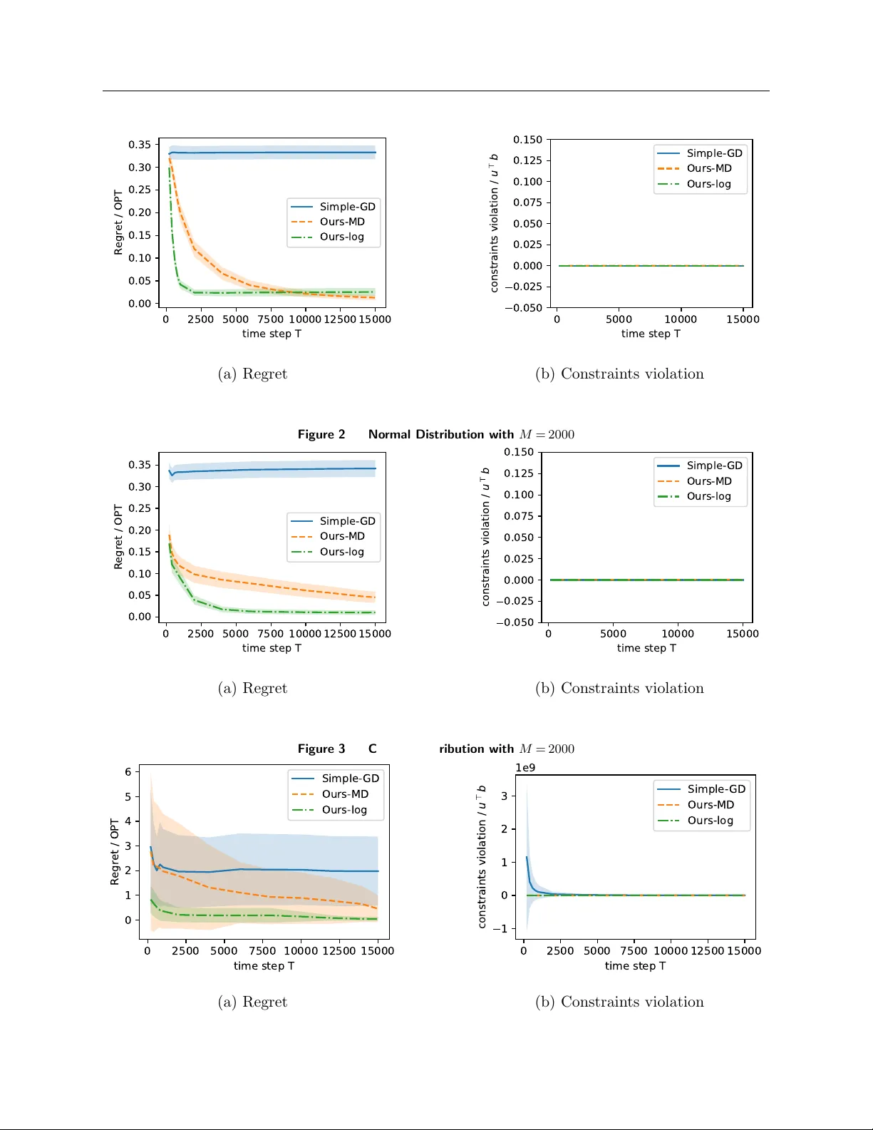
Online Semi-inﬁnite Linear Programming: Eﬃcien t Algorithms via F unction Appro ximation Yiming Zong † , Jiash uo Jiang † † Department of Industrial Engineering & Decision Analytics, Hong Kong Univ ersity of Science and T echnology W e consider the dynamic resource allo cation problem where the decision space is ﬁnite-dimensional, y et the solution must satisfy a large or even inﬁnite num b er of constraints revealed via streaming data or oracle feedbac k. W e mo del this challenge as an Online Semi-inﬁnite Linear Programming (OSILP) problem and dev elop a no vel LP form ulation to solv e it appro ximately . Sp eciﬁcally , we employ function approximation to reduce the num b er of constraints to a constant q . This addresses a key limitation of traditional online LP algorithms, whose regret b ounds typically dep end on the num b er of constrain ts, leading to p o or per- formance in this setting. W e propose a dual-based algorithm to solve our new form ulation, which oﬀers broad applicabilit y through the selection of appropriate p otential functions. W e analyze this algorithm un- der tw o classical input mo dels—sto chastic input and random p ermutation—establishing regret bounds of O ( q √ T ) and O  q + q log T ) √ T  resp ectiv ely . Note that b oth regret b ounds are independent of the num- b er of constraints, which demonstrates the p otential of our approach to handle a large or inﬁnite num b er of constraints. F urthermore, we inv estigate the p otential to improv e up on the O ( q √ T ) regret and prop ose a t wo-stage algorithm, ac hieving O ( q log T + q /ε ) regret under more stringen t assumptions. W e also extend our algorithms to the general function setting. A series of exp eriments v alidates that our algorithms outp erform existing methods when confronted with a large num b er of constraints. Key wor ds : Semi-inﬁnite Programming, Sublinear Regret, Online Optimization, Primal-dual Up date 1. In tro duction In this pap er, w e in v estigate the general problem of Online Semi-Inﬁnite Linear Programming (OSILP) ov er a ﬁnite horizon of discrete time p erio ds. This setting represen ts a signiﬁcant general- ization of classical online optimization: while the decision v ariables are ﬁnite-dimensional, the con- strain ts they must satisfy are dra wn from an inﬁnite or contin uous index set, revealed sequen tially . A t each time step t , the decision maker observes a sto chastic input ( r t , a t ), dra wn indep endently from an underlying distribution, and m ust immediately make a decision x t . The primary ob jective is to maximize the total cum ulativ e reward sub ject to the rev ealed constraints. Our formulation is motiv ated by the increasing prev alence of high-dimensional streaming data where constrain ts are not merely n umerous but eﬀectiv ely con tinuous. By bridging the gap betw een 1 2 online learning and semi-inﬁnite programming, our framework uniﬁes and extends a broad range of classical mo dels and mo dern applications: 1. Robust and Distributionally Robust Optimization : Our mo del naturally encapsulates robust linear programming with uncertain ty sets ( Ben-T al and Nemirovski 1998 , Bertsimas and Sim 2004 ) and distributionally robust optimization (DRO) problems inv olving generalized mo- men ts ( Delage and Y e 2010 , Moha jerin Esfahani and Kuhn 2018 ). In these settings, the “inﬁnite” constrain ts corresp ond to the w ors t-case scenarios within an uncertaint y set. 2. Spatio-T emp oral Resource Allo cation : In contin uous facilit y lo cation and p -cen ter–type co vering problems ( Drezner and Hamacher 2004 ), constrain ts are often spatially indexed ov er a con tinuous region. Similarly , in sp ectrum allo cation for wireless netw orks, interference constraints m ust be satisﬁed across a contin uous frequency band and spatial domain, whic h ﬁts our semi-inﬁnite framew ork. 3. Con trol Systems and Engineering : Scenario-based metho ds in control often rely on con- strain ts discov ered via streaming data ( Calaﬁore and Campi 2006 , Campi and Garatti 2008 ). Our mo del is applicable to real-time safety-critical control, where a system must maintain safet y margins (constrain ts) across a contin uous state space while optimizing p erformance. F urthermore, our form ulation generalizes the standard Online Linear Programming (OLP) prob- lem, which is recov ered when the constraint index set is ﬁnite. F ollowing the traditional online LP literature, we analyze our algorithms under t wo canonical settings: the Stochastic Input Mo del, where the input data ( r t , a t ) are generated i.i.d. from an unkno wn distribution P , and the Random P ermutation Mo del, where an adversary can ﬁx a ﬁnite collection S = { ( r t , a t ) } T t =1 b eforehand and then rev eal it in a uniformly random order. W e ev aluate p erformance using t wo metrics: r e gr et and c onstr aint violation . W e adopt the oﬄine optimal solution as our b enchmark, which assumes kno wledge of the en tire sequence ( r π ( t ) , a π ( t ) ) in adv ance to maximize the ob jective P t = 1 T r t x t . The regret measures the gap b etw een the oﬄine optimal ob jectiv e v alue and the decision maker’s cum ulative rew ard, while the constrain t violation measures the feasibility of our prop osed solution. 1.1. Main Results and Con tributions While many existing online LP algorithms rely on a primal–dual paradigm (e.g., Li et al. ( 2023 )), these metho ds cannot b e directly transferred to the semi-inﬁnite setting. In standard online LP , dual v ariables are updated via m ultiplicativ e w eigh ts or pro jection within a ﬁnite-dimensional Euclidean space. In contrast, the dual v ariable in an online semi-inﬁnite LP is a non-negative measure. Direct application of multiplicativ e w eights or gradien t descent is infeasible in this uncountably inﬁnite- dimensional space. Moreov er, their regret b ounds dep end on the num b er of constraints, which can b e inﬁnitely large under our setting. 3 T o o v ercome this dimensionalit y mismatc h, w e emplo y function approximation. A k ey inno v ation of our w ork is the utilization of non-ne gative b asis functions to parameterize the dual space. This approac h oﬀers tw o distinct adv antages: 1) it allows us to optimize ov er non-negative w eigh ts, a constrain t that is computationally straigh tforw ard to main tain during updates; and 2) the ob jectiv e v alue of the approximate problem serves as an upp er b ound to the original problem, simplifying the deriv ation of p erformance guarantees. Lev eraging this nov el formulation, we provide the following main con tributions. 1. A Simple Algorithm Design and Sublinear Regret Bounds : W e ﬁrst design a simple Gradien t Descen t algorithm for the sto chastic input mo del and then extend this to a general Mirror Descen t framework applicable to b oth sto chastic and random p ermutation mo dels. W e pro v e that our algorithm achiev es an O ( q √ T ) sublinear regret b ound under the sto chastic input mo del and an O (( q + q log T ) √ T ) regret b ound under the random p ermutation mo del, where q denotes the dimension of the basis functions. 2. An Impro ved Tw o-Stage Algorithm : Under a Global P olyhedral Gro wth (GPG) assump- tion with parameter ϵ , w e prop ose an enhanced tw o-stage algorithm. This metho d ﬁrst accelerates the conv ergence of the dual v ariable to a neighborho o d of the optimal solution, and subsequen tly reﬁnes it. This approach ac hieves an improv ed regret b ound of O ( q log T + q /ϵ ), signiﬁcantly out- p erforming the standard O ( q √ T ) rate. 3. Scalability via Constrain t-Cardinality-Independence : A central b ottleneck in extending standard online LP metho ds to semi-inﬁnite problems is the explicit dep endence on the constraint cardinalit y m . In particular, many classical online LP algorithms incur linear or p olynomial dep en- dence on m , whic h hinders their scalability . Our framew ork remo ves this dep endence by applying function approximation to the dual v ariable: instead of maintaining a p er-constrain t dual v ariable, w e approximate the non-negative dual measure using q -dimensional non-negativ e basis functions and update only their w eigh ts. Consequen tly , our regret bounds only dep end on q , whic h is a kno wn constan t and indep endent of m . This demonstrates the p otential of our algorithm for handling the semi-inﬁnite problems. W e compare our con tributions with important prior works under similar form ulation in the following T able 1 . In addition to the ab ov e-men tioned main contributions, w e extend our t wo online LP algorithms to a general function setting, where the ob jectiv e and constrain ts are go v erned by concav e func- tions f and conv ex function g rather than a linear parametrization, and analyze their theoretical guaran tees. Suc h an extension substantially broadens our algorithms’ applicability to nonlinear constrain ts or ob jectives and rich p olicy classes. Finally we conduct numerical exp erimen ts to demonstrate the sup erior p erformance of our algorithms, particularly in scenarios characterized b y a massiv e num b er of constraints where traditional metho ds struggle. 4 T able 1 Compa rison of our w ork to imp ortant prio r literature Mo del Regret Li and Y e ( 2022 ) sto c hastic input O ( m 2 log T log log T ) Li et al. ( 2023 ) sto c hastic input O ( m √ T ) random p erm utation O (( m + log T ) √ T ) Gao et al. ( 2025 ) sto c hastic input O ( m log T ) Our w ork sto c hastic input O ( q √ T ), O ( q log T + q ϵ ) random p erm utation O (( q + q log T ) √ T ) In summary , our w ork provides the ﬁrst algorithmic framew ork for solving the online semi-inﬁnite LP problems, and w e justify our algorithms b oth theoretically via rigorous performance guarantees and empirically through extensiv e numerical exp eriments. 1.2. Related Literature Semi-Inﬁnite Line ar Pr o gr amming Semi-Inﬁnite Linear Programming (SILP) addresses linear optimization problems with ﬁnite decision v ariables but inﬁnite inequalit y constrain ts. Classical SILP algorithms typically follow a ﬁnite-appro ximation–correction paradigm: solve a master prob- lem ov er a ﬁnite subset of constrain ts, then identify a new violating index and augmen t the active set. Several previous literature develops new algorithms based on the central cutting plane metho d ( Betro 2004 , Mehrotra and P app 2014 , Zhang et al. 2013 ), where any suﬃcien tly informative vi- olated or nearly tigh t constraint can generate an eﬀective cut. Recently , many literature fo cuses on the adaptiv e discretization ( Still 2001 , Mitsos 2011 , Jungen et al. 2022 , Reem tsen 2025 ). In addition, Oustry and Cerulli ( 2025 ) introduces a nov el metho d that employing an inexact oracle to handle con vex semi-inﬁnite programmings. Online Line ar Pr o gr amming/R esour c e A l lo c ation Online Linear Programming/resource allo ca- tion has long b een in v estigated and has v arious applications, such as displaying ad allo cation ( Meh ta et al. 2007 ), reven ue management ( T alluri and V an Ryzin 2006 , Jasin and Kumar 2012 , Jiang et al. 2025a ), cov ering and packing problems ( Buc h binder and Naor 2005 , 2006 , F eldman et al. 2010 ) and more. A classical and prev alent framew ork for designing algorithm is the dual- based method, where the decision is made based on an estimated dual prices. Some literature follo w the sample-then-price scheme, that is the algorithm samples an initial preﬁx to learn dual prices and then ﬁxes them for the rest of the horizon ( Dev anur and Ha y es 2009 , F eldman et al. 2010 , Molinaro and Ravi 2014 , Dev an ur and Jain 2012 ). In contrast, other literature adopt the dynamic price learning scheme, whic h re-solves and up dates prices p erio dically , improving robustness and tigh tening dep endence on horizon ( Agraw al et al. 2014 , Li and Y e 2022 , Chen and W ang 2015 ). In 5 addition, there are also some pap ers fo cusing on primal-guided metho ds ( Kesselheim et al. 2014 ) and ﬁrst-order metho d without rep eating solving dual price ( Agra wal and Dev an ur 2014 , Balseiro et al. 2020 ). Online Convex Optimization and Constr aine d V ariants. Our w ork is also related to online con- v ex optimization (OCO). In the standard OCO framework, the decision maker c ho oses the decision b efore observing the loss function, and then incurs loss. This model is mainly motiv ated b y mac hine learning applications such as online linear regression and online supp ort vector machines ( Hazan 2016 ). Compared with our setting, standard OCO t ypically adopts a w eaker static regret b ench- mark, where the comparator is ﬁxed ov er time. By con trast, our b enchmark is the oﬄine optimum of the realized instance, which mak es standard OCO algorithms and analyses not directly appli- cable. Several works study dynamic regret in non-stationary or adversarial environmen ts ( Besb es et al. 2015 , Hall and Willett 2013 , Jadbabaie et al. 2015 ), but they fo cus on unconstrained prob- lems. There is also a line of w ork on online conv ex optimization with constraints (OCOwC), where the constraint functions are either static ( Jenatton et al. 2016 , Y uan and Lamp erski 2018 , Yi et al. 2021 ) or i.i.d. ov er time ( Neely and Y u 2017 ). The extension to Mark o vian en vironmen t has also b een studied ( Jiang 2023 , Li et al. 2025 , Jiang and Y e 2024 ) under v arious metrics with v arious applications. T o the best of our kno wledge, existing OCOwC results do not allo w for a large or inﬁnite n umber of constraints, which is the problem we address in this pap er. 2. Problem F orm ulation W e consider the general online semi-inﬁnite LP , which takes the following form: max r ⊤ x s . t . A x ≤ b 0 ≤ x i ≤ 1 , i = 1 , ..., T (1) where the input data ( r t , a t ) arrives at eac h time step t and the right-hand-side b and time horizon T are known b eforehand. Here the dimension of columns of matrix A and vector b are inﬁnite and w e use m to denote it for conv enience. The dual of this semi-inﬁnite LP ( 1 ) is: min b ⊤ u + 1 ⊤ s s . t . A ⊤ u + s ≥ r u ≥ 0 , s ≥ 0 (2) F ollo wing traditional online LP literature, our pap er mainly discusses tw o types of mo dels: sto c hastic input mo del and random p ermutation mo del, and w e formally state the deﬁnitions for these t wo mo dels in the following: 6 Definition 1. The input data { ( r t , a t ) } T t =1 satisfy one of the follo wing standard mo dels: 1. ( Sto c hastic Input Mo del ) ( r t , a t ) are i.i.d. sampled from an unkno wn distribution P . 2. ( Random Perm utation Model ) The multiset { ( r t , a t ) } T t =1 is ﬁxed in adv ance and arrives in a uniformly random order. 2.1. Assumptions No w we in tro duce some basic assumptions throughout the pap er. W e assume that b oth input data { r t , a t } T t =1 and right-hand-side b = T d are b ounded. F urthermore, our pap er develops a new LP form ulation via function approximations with non-negative basis functions Φ ∈ R m × q ≥ 0 , whic h will b e sp eciﬁed later. In semi-inﬁnite LP , it is common to assume that the dual measure is ﬁnite, whic h can b e translated that the term a ⊤ t Φ and d ⊤ Φ are also bounded. W e formally conclude these assumptions in the follo wing: Assumption 1. F or al l t = 1 , ..., T , 1. ( Bounde d Data ) L et right-hand-size b = T d and ther e exist known c onstants r > 0 , a > 0 and d > d > 0 such that, r t ≤ r, ∥ a t ∥ ∞ ≤ a, d ≤ ∥ d ∥ ∞ ≤ d. 2. ( Finite Dual Me asur e ) With r esp e ct to the b asis function Φ , ther e exist p ositive c onstants 0 < D ≤ D and C > 0 such that, D ≤   d ⊤ Φ   ∞ ≤ D,   a ⊤ t Φ   ∞ ≤ C . 2.2. P erformance Measure F or a giv en sequence of input data S = { ( r t , a t ) } T t =1 , we denote the oﬄine optimal solution of the semi-inﬁnite LP ( 1 ) as x ∗ = ( x ∗ 1 , ...x ∗ T ) and the corresp onding optimal v alue as R ∗ T . Similarly , we denote the actual decis ion of eac h time step t as x t ( π ) for a ﬁxed p olicy π and the ob jectiv e v alue as R T ( π ). That is, R ∗ T = T X t =1 r t x ∗ t , R T ( π ) = T X t =1 r t x t ( π ) . Then w e can give the formal deﬁnition of the optimality gap: Reg T ( P , π ) = R ∗ T − R T ( π ) where P = ( P 1 , ..., P T ) are the unkno wn distribution of input data S = { ( r t , a t ) } T t =1 . F or the sto chas- tic input mo del, these distribution P = ( P 1 , ..., P T ) are all identical; while for the random p ermuta- tion mo del, each P t is the conditional empirical distribution of the yet-unseen items (i.e. sampling without replacemen t). F ollowing traditional online LP literature, we aim to ﬁnd an upper b ound 7 for the exp ectation of the optimality gap for all distributions P , and w e deﬁne this p erformance measure as r e gr et : Reg T ( π ) = sup P ∈ Ξ E [Reg T ( P , π )] F urthermore, we consider a supplementary p erformance measure: c onstr aints violation . In classical Online LP with a ﬁnite n umber of constrain ts, violation is t ypically measured b y the Euclidean norm of the residual vector. Ho wev er, in the semi-inﬁnite setting, the constraint index set is con tin- uous, rendering the standard Euclidean norm ill-deﬁned or computationally in tractable. T o address this, w e adopt a dual-based measurement approac h. Instead of c hecking p oin t wise violation, w e measure the magnitude of violation “tested” against our dual basis functions. This concept draws from the weak duality in functional analysis, where a constraint is considered satisﬁed if its inte- grated v alue against all v alid test functions is non-p ositive. Let U = {∥ u ∥ 2 ≤ u : u = Φ w ≥ 0 } denote the domain of v alid dual test functions within the span of our non-negative basis Φ. W e formally deﬁne the c onstr aint violation as the worst-case w eighted violation o ver this set: v ( π ) = max u ∈U E h ||  u ⊤ ( A x ( π ) − b )  + || 2 i . 3. The new LP form ulation via F unction Appro ximation Large-scale problems remain challenging due to their complexit y and the high computational cost of solving them directly , where function appro ximation has been recen tly inv estigated as a p o w erful to ol to handle these issues (e.g., Liu et al. ( 2022 ), Jiang et al. ( 2025b )). In this section, w e in tro duce our new LP formulation via function appro ximation for the c hallenging OSILP problems. Denote the optimal solutions to the primal LP ( 1 ) and dual LP ( 2 ) as x ∗ , u ∗ and s ∗ . According to the complemen tary slackness, we hav e the following equations: x ∗ t = ( 1 , r t > a ⊤ t u ∗ 0 , r t < a ⊤ t u ∗ and s ∗ t = [ r t − a ⊤ t u ∗ ] + (3) for t = 1 , ..., T , and x t can b e an arbitrary v alue b e t ween 0 and 1 when r t = a ⊤ t u ∗ . Therefore, it is suﬃce to mak e a decision x t if the decision maker can obtain the accurate v alue of u ∗ . Note that the dimension of dual v ariable u ∗ is also inﬁnite, so we use function approximation to approximate it. T o b e sp eciﬁc, we assume that there exists a v ariable z such that the dual v ariable u can b e w ell approximated in the following formulation: u ( z ) ≈ q X k =1 ϕ ( z ) k w k = Φ w (4) A key step is that we use non-ne gative b asis functions (e.g. Radial Basis F unctions) to construct the basis function Φ. This technique brings sev eral b eneﬁts. First, for an arbitrary basis function 8 Φ, whic h ma y ha v e b oth negativ e and p ositive elements, it is non-trivial to pro ject the weigh t w in to the feasible set Φ w ≥ 0 during the up date pro cess. How ever, if we choose non-ne gative b asis functions , w ≥ 0 is a suﬃcient condition to satisfy the original constraint Φ w ≥ 0, and pro jecting w into non-negative sets is trivial. Second, although these t wo constraints are not equiv alent and there exists a gap b etw een optimal v alues of these t wo problems, w e can sho w that such a gap do es not aﬀect our ﬁnal regret upp er b ound. More sp eciﬁcally , let k := Φ w . Since basis function Φ may not constitute an orthogonal basis for the space R m ≥ 0 , the domain for k is K ⊆ R m ≥ 0 ; while the domain for the original dual v ariable u is exactly R m ≥ 0 . In other w ords, the domain of our appro ximate v ariable via basis function Φ is a subset of the domain of our target. Let d = b T and combine function approximations ( 4 ) and complementary slac kness ( 3 ), we can construct the follo wing problem, which is actually an approximate to the original dual LP ( 2 ): min w f T , Φ ( w ) = d ⊤ Φ w + 1 T T X t =1 ( r t − a ⊤ t Φ w ) + s . t . w ≥ 0 (5) Assume that the column-co eﬃcient pair ( r t , a t ) are sampled from some unknown distribution P and w e can consider ﬂuid relaxation: min w f Φ ( w ) = d ⊤ Φ w + E ( r,a ) ∼P  ( r − a ⊤ Φ w ) +  s . t . w ≥ 0 (6) F rom another p ersp ective, problem ( 5 ) can also b e view ed as the sample av erage approximation of the sto chastic problem ( 6 ). Applying similar idea to the dual problem ( 2 ), we can obtain the follo wing sto c hastic problem: min u f ( u ) = d ⊤ u + E ( r,a ) ∼P  ( r − a ⊤ u ) +  s . t . u ≥ 0 (7) Denote w ∗ as the optimal solution for the approximate dual problem ( 5 ) and u ∗ is the optimal solution for the ﬂuid relaxation dual LP ( 7 ), and the follo wing lemma help us build a bridge b etw een f ( u ∗ ) and f T , Φ ( w ∗ ): Lemma 1 (forklore) . It holds that f T , Φ ( w ∗ ) ≥ f ( u ∗ ) . Note that our goal is to ﬁnd an upp er b ound for regret and constraints violation, Lemma 1 naturally bridges the original optimal v alue f ( u ∗ ) to the appro ximate optimal v alue f T , Φ ( w ∗ ), and from no w on we can simply fo cus on dealing with problem ( 6 ) and f T , Φ ( w ∗ ). 9 4. A Dual-based First-order Algorithm W e b egin with a data-driv en ﬁrst-order algorithm under the sto c hastic input mo del and later w e extend it to a more general version under both the stochastic input mo del and the random p erm utation mo del. The formal deﬁnition of stochastic input model is presented in Deﬁnition 1 and our main algorithm is presen ted in Algorithm 1 . Our algorithm is motiv ated from the dual-based algorithm, that is, in each time step t , the algorithm makes a decision x t according to the optimal dual v ariable p ∗ , which is appro ximated by Φ w t in our algorithm. Then w e update w t to adju st our appro ximation to p ∗ using the sub-gradien t descen t method, and pro ject it in to the non-negative set. The up date ( 5 ) is the sub-gradien t of t -th term ev aluated at w t : ∂ w  d ⊤ Φ w + ( r t − a ⊤ t Φ w ) +    w = w t = d ⊤ Φ − a ⊤ t Φ I ( r t > a t Φ w )   w = w t = d ⊤ Φ − a ⊤ t Φ x t where the last equation uses the deﬁnition of x t in Step 4 of Algorithm 1 . Algorithm 1 Main algorithm 1: Input: d = b T . 2: Initialize w 1 = 0. 3: for t = 1 , ...T do 4: Observ e input data ( r t , a t ) and set x t = ( 1 , r t > a ⊤ t Φ w t 0 , r t ≤ a ⊤ t Φ w t 5: Up date w t +1 = Q w ≥ 0 [ w t + γ t ( a ⊤ t Φ x t − d ⊤ Φ) ] 6: end for 7: Output : x = ( x 1 , ...x T ). No w we provide another p ersp ective to illustrate Algorithm 1 . Consider the following LP: max r ⊤ x s . t . Φ ⊤ A x ≤ Φ ⊤ b 0 ≤ x t ≤ 1 , t = 1 , ..., T (8) Compared with the original primal formulation ( 1 ), the constrain t system in ( 8 ) is obtained b y pro jecting the original constrain ts on to the subspace spanned by Φ. Hence, ( 8 ) can be viewed as a constrain t-reduced (or pro jected) surrogate of ( 1 ): it ac hieves the approximate ob jective but 10 replaces the p otentially large set of constraints by a lo w er-dimensional set enco ded through Φ ⊤ A and Φ ⊤ b . The dual of ( 8 ) coincides with the appro ximate dual problem ( 5 ) b y identifying d = b T , where the asso ciated dual v ariable is w . Under this in terpretation, Algorithm 1 can b e view ed as a standard primal–dual metho d for solving the pro jected LP ( 8 ): the primal up date seeks to improv e the rew ard under the reduced constraints, while the dual up date adjusts w to p enalize violations of Φ ⊤ A x ≤ Φ ⊤ b . This p ersp ectiv e will b e useful for relating the algorithmic iterates to b oth the appro ximate dual ob jectiv e and the exten t of constrain t satisfaction in the original space. Before presen ting our formal result, w e ﬁrst illustrate that the dual v ariable w t is upper b ounded during the update, which is presented in Lemma 2 . Lemma 2 is highly dep endent on Assumption 1 , and its main purp ose is to help us deriv e an upp er b ound for constraints violation. Lemma 2. Under the sto chastic input mo del, if the step size γ t ≤ 1 for t = 1 , ..., n in Algorithm 1 , then || w t || 2 ≤ q ( C + D ) 2 + 2 r t 2 D + q ( C + D ) (9) wher e w t ’s ar e sp e ciﬁe d in A lgorithm 1 . No w we presen t our main result in Theorem 1 and lea ve the full pro of to app endix. Such a O ( √ T ) regret b ound has b een ac hieved in previous online LP literature, ho wev er, most of their results are also linear dep endent on the constraint dimension m , which leads to p o or p erformance confron ted with large or even inﬁnite constrain ts. Our algorithm is the ﬁrst to ac hieve a O ( q √ T ) regret b ound under the online SILP setting and our b ound is only dep endent on the dimension of w eight w , which is controllable and small in real applications. Theorem 1. Under the sto chastic input assumption and Assumption 1 , if step size γ t = 1 √ T for t = 1 , .., T in Algorithm 1 , the r e gr et and exp e cte d c onstr aints violation of Algorithm 1 satisfy R e g T ( π ALG1 ) ≤ O ( q √ T ) and v ( π ALG1 ) ≤ O ( q 2 √ T ) . 5. Mirror-Descen t-Based Metho d 5.1. Sto c hastic Input Mo del In this subsection, w e extend the Algorithm 1 to a mirror-descen t-based algorithm and discuss its regret bound under b oth sto chastic input mo del and random p ermutation mo del. F or a giv en p oten tial function ψ , we denote by D ψ ( u || v ) the corresp onding Bregman divergence, deﬁned as D ψ ( u || v ) = ψ ( u ) − ψ ( v ) − ⟨∇ ψ ( v ) , u − v ⟩ . Note that when choosing ψ ( u ) = 1 2 ∥ u ∥ 2 2 , the Mirror Descent will degenerate to the standard gradient descen t. Ho wev er, there are several sc enarios that c ho osing other potential functions are better. 11 F or instance, negative entrop y function ψ ( u ) = − P n i =1 u i log u i has b etter p erformance for the sparse solution LP problem. Therefore, dev eloping a Mirror Descent Based algorithm is of vital imp ortance. Before presenting our formal algorithm, w e ﬁrst introduce a standard assumption for the p otential function ψ , together with a b oundedness assumption on the dual iterates w t . W e assume that ψ is coordinate-wisely separable and α -strongly conv ex with respect to a giv en norm, a setting that co vers many commonly used p oten tial functions. When mirror descen t reduces to Euclidean pro jection, (i.g. ψ ( u ) = 1 2 u 2 ) we ha ve already established that the dual v ariables w t admit an upp er b ound throughout the iterations. How ever, for a ge neral p oten tial function, it is typically not possible to deriv e an explicit or closed-form upp er b ound for the dual v ariables in the same wa y as in the Euclidean case. In light of this diﬃculty , we in tro duce a more general assumption that the dual v ariables remain b ounded ov er the course of the algorithm’s up dates once the p otential function is determined. Assumption 2 (Mirror map and b ounded dual iterates) . The p otential function ψ ( u ) is c o or dinate-wisely sep ar able, that is, ψ ( u ) = P p j =1 ψ j ( u j ) wher e ψ j : R + → R is an univariable func- tion and α -str ongly c onvex with r esp e ct to a given norm ∥·∥ . Mor e over, the dual variable gener ate d by Algorithm 2 r emains uniformly b ounde d thr oughout the iter ations: ther e exists a known c onstant W such that ∥ w t ∥ ∞ ≤ W . W e presen t our formal algorithm in Algorithm 2 , which is mainly based on Algorithm 1 with the modiﬁcation on the update form ula for dual v ariable w t . No w w e discuss the regret b ound of Algorithm 2 under sto chastic input model ﬁrst, whic h is given in Theorem 2 . Our b ound is dep enden t on the concrete p oten tial function ψ with resp ect to a norm || · || . T o b ound these arbitrary norm, we giv e the upp er b ound under the l 2 norm. Therefore for an y given norm || · || , || g t || 2 ∗ will alw a ys ha v e an upp er b ound, which is a constan t m ultiple dep ending on that particular norm and the dimension. In our ﬁnal bound, w e omit this term and obtain the O ( q √ T ) regret b ound. Theorem 2. Under the sto chastic input mo del, Assumption 1 , and Assumption 2 , if step size γ t = 1 √ T for t = 1 , .., T in Algorithm 2 , the r e gr et and exp e cte d c onstr aints violation of A lgorithm 2 satisfy R e g T ( π ALG2 ) ≤ O ( q √ T ) and v ( π ALG2 ) ≤ O ( p q T ) . 5.2. Random Perm utation Mo del In this subsection, we discuss a more general setting: Random Perm utation Mo del. In this mo del, co eﬃcien t pair ( r t , a t ) arrives in a random order and their v alue can b e chosen adversarially at 12 Algorithm 2 Mirror-descent-based algorithm 1: Input: d = b T . 2: Initialize w 1 = 0. 3: Parameters: p otential function ψ ; step size γ t 4: for t = 1 , ..., T do 5: Observ e input data ( r t , a t ) and set x t = ( 1 , r t > a ⊤ t Φ w t 0 , r t ≤ a ⊤ t Φ w t 6: Up date g t = d ⊤ Φ − a ⊤ t Φ x t . 7: Up date w t +1 = arg min w ≥ 0 {⟨ γ t g t , w ⟩ + D ψ ( w || w t ) } . 8: end for 9: Output : x = ( x 1 , ...x T ). the start. T o simplify the exp osition and exclude degeneracy , we w ork under a standard general- p osition conv ention. In particular, following the common p erturbation argumen t ( Dev anur and Ha yes 2009 ), one may indep endently p erturb each reward r i b y an arbitrarily small contin uous noise term (e.g. ϵ ∼ U[0 , β ]). Since the dual v ariable w t lies in R q ≥ 0 , no vector w t can satisfy more than q indep endent equalities simultaneously; consequently , after this p erturbation, with probability one that an y w can only satisfy at most q independent equations at the same time. Hence, this non-degeneracy condition can b e imp osed without loss of generality . Under this conv ention, w e can deﬁne the follo wing thresholding rule: x i ( w ∗ ) = ( 1 , r i > a ⊤ i Φ w ∗ 0 , r i ≤ a ⊤ i Φ w ∗ (10) where x ( w ∗ ) = ( x 1 ( w ∗ ) , ..., x n ( w ∗ )). Lemma 3. Denote x ∗ i as the optimal solution for the appr oximate primal LP r elaxation ( 8 ) and x i ( w ∗ ) is deﬁne d in ( 10 ) , then we have x i ( w ∗ ) ≤ x ∗ i for al l i = 1 , ..., n . Besides, under the gener al- p osition c onvention ab ove, x i ( w ∗ ) and x ∗ i diﬀers for no mor e than q values of i . Denote the optimal v alue of approximate primal LP ( 8 ) R ∗ Φ . Lemma 3 tells us that the diﬀerence of P n i =1 r i x i ( w ∗ ) and R ∗ Φ can b e b ounded by q r . That is, | n X i =1 r i x i ( w ∗ ) − R ∗ Φ | ≤ q r Then w e consider a scaled version of the approximate primal LP relaxation ( 8 ): max s X i =1 r ⊤ i x i s . t . s X i =1 a ⊤ j i x i ≤ sb j T , 0 ≤ x ≤ 1 (11) 13 for s = 1 , .., T . Denote the optimal v alue of scaled version of the approximate primal LP ( 8 ) R ∗ s . The follo wing prop osition helps us relate R ∗ s to R ∗ Φ : Proposition 1. F or s > max { 16 C 2 , e 16 C 2 , e } ,the fol lowing ine quality holds: 1 s E [ R ∗ s ] ≥ 1 T R ∗ Φ − q r T − r log s D √ s − q r s (12) for al l s ≤ T ∈ N + . No w we present our formal result in Theorem 3 . Since Random Perm utation Mo del is a more c hallenging than under the Sto chastic Input Mo del, our regret b ound is w eaker than prior results; ho wev er, these tw o settings exhibit comparable p erformance in terms of constraint violations. Theorem 3. Under the r andom p ermutation mo del, Assumption 1 , and Assumption 2 , if step size γ t = 1 √ T for t = 1 , .., n in Algorithm 2 , then the r e gr et and exp e cte d c onstr aints violation satisfy R e g T ( π ALG2 ) ≤ O  ( q + q log T ) p q T  and v ( π ALG2 ) ≤ O ( p q T ) wher e || · || ∗ denotes the dual norm of || · || and g t satisﬁes || g t || 2 2 ≤ q ( C + D ) 2 . 6. Ac hieving log T Regret In previous sections, w e ha ve in tro duced tw o ﬁrst order algorithms achieving O ( q √ T ) regret b ound. Ho wev er, can w e dev elop a more eﬃcient algorithm outp erforming O ( q √ T ) regret under the sto c hastic input mo del? The answer is yes . In this section, w e will prop ose a no vel algorithm that achiev es O ( q log T + q ε ) regret, exceeding previous O ( m √ T ) regret b ound in most literature. This nov el algorithm has t wo stages: i) accelerating stage, rapidly driving the iterates into a neigh b orho o d of the optimal solution; ii) reﬁnemen t stage, applying ﬁrst order metho ds to reﬁne the solution and ensure accurate optimalit y . Before formally presen ting the algorithm, w e ﬁrst introduce t wo common and imp ortant assumptions, whic h play key roles in our later analysis: Assumption 3 (General Position Gap) . Denote w ∗ as the unique optimal solution of ( 6 ) . L et B ϵ ( d ) b e the b al l c enter e d at d with r adius ϵ under the ℓ 2 norm, i.e., B ϵ ( d ) = { ˆ d : ∥ ˆ d − d ∥ 2 ≤ ϵ } . Ther e exists ϵ > 0 such that for al l ˆ d ∈ B ϵ ( d ) , w ∗ r emains the optimal solution. Note that this General P osition Gap (GPG) assumption is equiv alent to the general non- degeneracy assumption. The general non-degeneracy assumption mainly includes following tw o parts: i) F or a given RHS vector d the primal LP admits a unique optimal basic solution; ii) 14 This optimal basis is nondegenerate, which means all basic v ariables, including the asso ciated slac k v ariables, are strictly p ositive ( i.e., no basic v ariable is equal to zero). F rom the geometric p ersp ectiv e, this means that the RHS vector d do es not lie on the degeneracy b oundary of the feasible region; instead, it lies in the in terior of a well-behav ed region in which the optimal basis is unique and stable. Therefore, there must exist ε > 0 such that as long as d falls into a small region B ϵ ( d ) = { ˆ d : ∥ ˆ d − d ∥ 2 ≤ ϵ } , this unique optimal basic solution remains optimal, whic h is exactly equiv alent to our GPG deﬁnition. Assumption 4 (H¨ older Error Bound) . F or al l w ≥ 0 , ther e exist some λ > 0 and θ ∈ (0 , 1] such that f ( w ) − f ( w ∗ ) ≥ λ · dist ( w , W ∗ ) 1 /θ wher e dist ( w , W ∗ ) = inf ∥ w − w ∗ ∥ and W ∗ is the optimal set for pr oblem ( 8 ) . This H¨ older Error Bound assumption c haracterizes an upp er b ound when the p oint is a wa y from the optimal set. In p olyhedral settings such as linear programming, this prop erty t ypically follows from Hoﬀman-t yp e error b ounds and thus holds under mild regularit y assumptions. The dual error b ound is a key regularity condition in conv ergence analysis: it allows one to conv ert the deca y of a residual or ob jectiv e gap in to a corresp onding decrease in the distance to the dual solution set, whic h in turn facilitates linear con vergence guarantees for ﬁrst order algorithms. 6.1. Accelerate Stage W e now introduce the ﬁrst part of our algorithm: the Accelerate stage. In traditional ﬁrst-order metho ds, the initial p oint is often set to w 1 = 0 and is frequen tly far from the optimal solution w ∗ , whic h typically leads to slow con vergence. T o address this issue, we emplo y an accelerated gradient descen t metho d to guide the initial p oint to a neighborho o d of the optimal solution in as few steps as p ossible. The formal algorithm is presen ted in Algorithm 3 . Note that our Algorithm 3 main tains tw o v ariables: w t and ˜ w l j . The accelerated gradien t descent mec hanism ensures that ˜ w l j con verges rapidly to a near-optimal solution. The k ey p oint of this step is that w e not only pro ject w t on to R ≥ 0 but also on to a ball whose radius is updated sync hronously , whic h helps to limit any oscillations that w t ma y exp erience during the up date pro cess. Since w t gets closer to the optimal v alue with each up date, w e treat the previous w t as the center of the ball for the next up date and sim ultaneously decrease the radius of the pro jection ball to ensure that w t con verges rapidly to a region around the optimal v alue while minimizing oscillations and impro ving stability . How ever, this fast con vergence has no guarantee to wards the regret of decision making and may sometimes result in bad p erformance. T o address this issue, we also maintain the v ariable w t to more reliably appro ximate the optimal dual v ariable while making decisions. 15 Algorithm 3 F ast Conv ergence Algorithm - Accelerate Sto c hastic Subgradien t Metho d 1: Input: d = b T , total time horizon T , probabilit y δ , initial error estimate ε 0 = r D . 2: Set L = ⌈ log ( ε 0 T ) ⌉ , ˆ δ = log δ K , J ≥ max { 9( C + D ) 2 λ 2 , 1152( C + D ) 2 log (1 / ˆ δ ) λ 2 } and T fast = L · J 3: Initialize w 0 = ˜ w 0 = 0; step size η 1 = ε 0 3 r 2 and γ t = 1 log T ; V 1 ≥ ε 0 λ ; B 0 = b ⊤ Φ. 4: for l = 1 , ...L do 5: Set ˜ w l 1 = ˜ w l − 1 and domain K = R ≥ 0 ∩ B ( ˜ w l − 1 , V k ). 6: for j = 1 , ...J do 7: Compute curren t time step t = ( l − 1) ∗ J + ( j − 1). 8: Observ e input data ( r t , a t ) and set ˜ x t = ( 1 , r t > a ⊤ t Φ w t 0 , r t ≤ a ⊤ t Φ w t 9: Set x t = ˜ x t · I { a ⊤ t Φ ˜ x t ≤ B t } 10: Up date B t +1 = B t − a ⊤ t Φ x t 11: Up date w t +1 = max { w t + γ t ( a ⊤ t Φ ˜ x t − d ⊤ Φ) , 0 } 12: Up date ˜ w l j +1 = Q K  ˜ w l j + η l ( a ⊤ t Φ ˜ x t − d ⊤ Φ )  13: end for 14: Set ˜ w l = 1 J P J j =1 ˜ w l j . 15: Set η l +1 = η l 2 and V l +1 = V l 2 . 16: end for 17: Output : ( x 1 , ..., x T fast ) , ˜ w L , T fast . Another distinctiv e feature of Algorithm 3 compared to previous metho ds is the handling of constrain ts in Steps 9. In this part of the algorithm, the pro cedure ensures that all constraints are contin uously satisﬁed throughout the pro cess. This is crucial b ecause, unlike in traditional algorithms where constrain ts may o ccasionally b e violated, Algorithm 3 guaran tees that constrain ts are satisﬁed at all times, th us impro ving the robustness and reliabilit y of our decisions. Theorem 4. Under the sto chastic input mo del, Assumption 1 , and Assumption 4 , supp ose w ∗ is the optimal solution for the pr oblem ( 8 ) , the output of A lgorithm 3 satisﬁes that ∥ ˜ w L − w ∗ ∥ ≤ 1 T with high pr ob ability 1 − δ . In addition, the r e gr et of A lgorithm 4 until l time T fast satisﬁes that R e g T fast ( π ALG3 ) ≤ O ( q log T ) . 16 6.2. Reﬁne Stage No w w e comes to the second stage and presen t it in Algorithm 4 . The k ey inno v ation of Algorithm 4 compared to previous algorithms lies in its use of an initial dual v ariable that is a near-optimal solution to the ﬂuid relaxation problem, rather than starting from 0 as in prior approaches. In this w ay , the algorithm do es not waste time conv erging from an arbitrary starting p oint and maintain more accurate solutions throughout. F urther, this adaptive design also oﬀers a signiﬁcant adv an tage o ver directly using the exp ected optimal solution, whic h is known to b e an O ( √ T ) regret. By dynamically adjusting based on the observed data at each step, the algorithm av oids rigidly relying on a ﬁxed exp ectation, allowing it to resp ond more ﬂexibly to v ariations in the data. This approach ensures that the algorithm remains closely aligned with underlying problem dynamics, preven ting large deviations from exp ected optim um and resulting in a substantial improv emen t in our constan t regret bound. In addition, Algorithm 4 also adopts a virtual decision ˜ x t as in Algorithm 3 to ensure that all constrain ts are satis ﬁed and maintain the ov erall consistency of the ﬁnal algorithm. Algorithm 4 Reﬁne Algorithm 1: Input: d = b T , near optimal dual solution ˆ w ∗ , T reﬁne = T − T fast . 2: Parameters: step size γ t . 3: Initialize w 1 = ˆ w ∗ and B 1 = d ⊤ Φ · T . 4: for t = 1 , ...T reﬁne do 5: Observ e input data ( r t , a t ) and set: ˜ x t = ( 1 , r t > a ⊤ t Φ w t 0 , r t ≤ a ⊤ t Φ w t 6: Set x t = ˜ x t · I { a ⊤ t Φ ˜ x t ≤ B t } 7: Up date w t +1 = max { w t + γ t ( a ⊤ t Φ ˜ x t − d ⊤ Φ ) , 0 } 8: Up date B t +1 = B t − a ⊤ t Φ x t 9: end for 10: Output : w = ( w 1 , ... w T reﬁne ). The following Theorem 5 gives the regret b ound of Algorithm 4 and the full pro of is presen ted in Section D.3 . Theorem 5. Under the sto chastic input mo del, Assumption 1 , and Assumption 3 , if sele cting step size γ t ≤ 1 T for t = T fast + 1 , ..., T , the r e gr et of Algorithm 4 satisﬁes R e g T r eﬁne ( π ALG4 ) ≤ O  q ε  . 17 6.3. Putting it together In the previous sections, we hav e discussed the t w o distinct stages of our algorithm. No w, w e in tegrate them into a uniﬁed framework, whic h is outlined in Algorithm 5 . In Algorithm 3 , we ha ve obtained a near-optimal solution with an O (log T ) regret b ound using O (log T ) time steps. This solution is then fed in to Algorithm 4 , which further reﬁnes the dual v ariable w t within the remaining time and ac hieves a constan t regret. By combining the strengths of these t w o algorithms, w e successfully achiev es a O (log T + 1 /ε ) regret b ound, b eating previous O ( √ T ) regret. W e present our ﬁnal result in Theorem 6 , whic h is an immediate result combining Theorem 4 and Theorem 5 . Algorithm 5 Accelerate-Then-Reﬁne Algorithm 1: Input: d = b T , time horizon T . 2: Compute T fast and T reﬁne = T − T fast . 3: for t = 1 , ...T fast do 4: Run Accelerate Algorithm 3 . 5: end for 6: for t = T fast + 1 , ...T do 7: Run Reﬁne Algorithm 4 . 8: end for 9: Output : x = ( x 1 , ...x T ), w = ( w 1 , ... w T ). Theorem 6. Under the sto chastic input mo del, Assumption 1 , Assumption 3 with p ar ameter ε and Assumption 4 , if sele cting step size γ t = 1 log T for t = 1 , ..., T fast and γ t ≤ 1 T for t = T fast +1 ,...,T in A lgorithm 5 , the r e gr et of A lgorithm 5 satisﬁes that with high pr ob ability 1 − δ : R e g T ( π ALG5 ) ≤ O  q log T + q ε  . 7. Extension to General F unction Settings In previous sections, we ha ve prop osed t wo ﬁrst-order algorithms for online linear programming. No w we extend our algorithms to a more general setting: at eac h time step t , we observe a reward function f ( x t ; θ t ) : X → R and cost functions g ( x t ; θ t ) : X → R m , where X is a con v ex and compact set and θ t ∈ Θ ⊂ R l is the parameter to b e revealed at time t . In particular, when θ t = ( r t , a t ) the optimization problem reduces to the online LP problem discussed in the previous sections. W e now formally presen t this general function setting in the b elow: 18 max T X t =1 f ( x t ; θ t ) s . t . T X t =1 g i ( x t ; θ t ) ≤ b i x ∈ X (13) Similar to Assumption 1 , w e mak e following assumptions throughout the whole section: Assumption 5. Without loss of gener ality, we assume that i) The functions f ( x t ; θ t ) ar e c onc ave over al l x t ∈ X and g ( x t ; θ t ) ar e c onvex over al l x t ∈ X for al l p ossible θ t ∈ Θ . ii) | f ( x t ; θ t ) | ≤ F for al l x t ∈ X , θ t ∈ Θ . iii)   g ( x t ; θ t ) ⊤ Φ   ∞ ≤ G for al l x t ∈ X , θ t ∈ Θ . In addition, 0 ∈ X and g i (0; θ ) = 0 for al l θ ∈ Θ . iv) θ t ar e i.i.d. sample d fr om some distribution P . v) Ther e exist two p ositive c onstants D and D such that, D ≤   d ⊤ Φ   ∞ ≤ D . W e deﬁne the following exp ectation for and a probability measure P in the parameter space Θ, W e then ev aluate the function u ( x ; θ ) : X → R in exp ectation ov er Θ by deﬁning the op erator P u ( x ( θ t ); θ ) = Z θ ′ ∈ Θ u ( x ( θ ′ t ); θ ′ ) d P ( θ ′ ) where x ( θ ) : Θ → X is a measurable function. This construction aggregates the v alues u ( x ( θ ′ t ); θ ′ ) across the parameter space according to P . Consequently P u ( · ) can b e in terpreted as a deterministic functional: giv en the mapping x ( · ), it returns a single scalar obtained b y a veraging with resp ect to the underlying parameter distribution. With this op erator in place, w e next introduce a function that c haracterizes the optimization problem once the parameter θ t has b een observ ed. s ( w ; θ t ) = max w ≥ 0 { f ( x ( θ t ); θ t ) − g ( x ( θ t ); θ t ) ⊤ Φ w } Then we can directly apply our new reformulation in Section 3 and obtain the follo wing appro xi- mation: min w h T , Φ ( w ) = d ⊤ Φ w + 1 T T X t =1 P t s ( w ; θ t ) s . t . w ≥ 0 (14) where x ( θ t ) = ( x 1 ( θ t ) , ..., x t ( θ t )) are primal decisions. Note that all primal decisions x ( θ t ) are dep enden t on the parameter θ t since our algorithm alwa ys observes new input data ﬁrst and then mak e a decision. 19 7.1. Mirror-Descen t-Based Algorithm In this subsection w e extend our Algorithm 2 to this general function settings and we present it in Algorithm 6 . This extension highligh ts that the core mechanism of our approach is not tied to the linear programming structure, but instead relies on the mirror-descent template with a suitable c hoice of p otential function ψ . Therefore we omit the extension of Algorithm 1 , as it can b e viewed as a sp ecial case of Algorithm 2 when selecting ψ ( u ) = 1 2 ∥ u ∥ 2 2 . Moreo v er, in Section 5 w e ha v e made t w o additional common assumptions and we will not rep eat them here to av oid redundancy . Compared with the linear case, the main tec hnical subtlety in this general function setting lies in Step 4: we no w need to ﬁnd some x to maximize function s ( x ; θ ), while in the linear case w e can immediately ﬁnd that x = 1 is the optimal solution to this optimization problem. Algorithm 6 Mirror-descent-based algorithm under general function setting 1: Input: d = b T . 2: Initialize w 1 = 0. 3: for t = 1 , ...T do 4: Observ e input parameter θ t and solv e x t = arg max x ∈X { f ( x ; θ t ) − g ( x ; θ t ) ⊤ Φ w t } (15) 5: Up date y t = d ⊤ Φ − g ( x t ; θ t ) ⊤ Φ x t . 6: Up date w t +1 = arg min w ≥ 0 {⟨ γ t y t , w ⟩ + D ψ ( w || w t ) } . 7: end for 8: Output : x = ( x 1 , ... x T ). Imp ortan tly , Algorithm 6 ac hieves the same order of regret bound as in the linear case. This sho ws that our analysis do es not hinge on linearit y , and that the performance guaran tee carries o ver to a signiﬁcan tly broader class of ob jectives and constrain t structures. In other words, the linear- programming formulation should be view ed as an instantiation of a more general metho dology rather than a restriction of our framew ork. W e formalize our result in the following: Theorem 7. Under the sto chastic input mo del, Assumption 2 and Assumption 5 , if the step size γ t = 1 √ T for t = 1 , .., T in Algorithm 6 , the r e gr et and exp e cte d c onstr aints violation of A lgorithm 6 satisfy R e g T ( π ALG6 ) ≤ O ( q √ T ) and v ( π ALG6 ) ≤ O ( p q T ) . 20 7.2. Tw o Stage Algorithm No w w e extend our t w o stage algorithm in to the general function settings and present it in Algo- rithm 7 . Before analyzing its p erformance, we ﬁrst establish an upp er b ound for the dual v ariables w t generated in Algorithm 7 . Concretely , w e pro ve that ∥ w t ∥ 2 remains bounded b y a problem- dep enden t constan t that do es not grow with t or T . This b oundedness result is crucial: it preven ts the dual iterates from explo ding, ensures that the primal up dates are p erformed with well-con trolled eﬀectiv e step sizes, and allo ws us to b ound the magnitude of the terms in the Lagrangian that in volv e the dual v ariables w t , whic h app ear in the regret decomp osition. Lemma 4. Under Assumption 5 , the dual variable w t in A lgorithm 7 c an b e upp er b ounde d by || w t || 2 ≤ q ( G + D ) 2 + 4 F 2 D + q ( G + D ) (16) Building on this boundedness property , w e no w analyze the regret of Algorithm 7 . Using the same t w o-stage decomp osition as in Algorithm 5 , w e sho w that the cumulativ e error terms con- tributed by the primal and dual updates can b e dominated b y a logarithmic function of the horizon. As a result, Algorithm 7 achiev es an log T regret bound in the general function setting as well, demonstrating that the improv ed regret guarantee is not an artifact of linearity but a consequence of the algorithmic structure and the stabilit y of the dual sequence. Theorem 8. Under the sto chastic input mo del, Assumption 3 with p ar ameter ε , Assumption 4 and Assumption 5 , if sele cting step size γ t = 1 log T for t = 1 , ..., T fast and γ t ≤ 1 T for t = T fast +1 ,...,T in A lgorithm 5 , the r e gr et of A lgorithm 7 satisﬁes that with high pr ob ability 1 − δ : R e g T ( π ALG7 ) ≤ O ( q log T + q ε ) . 8. Numerical Exp erimen ts 8.1. Exp erimen t Setup A key step in our algorithm is the use of non-ne gative basis and now we explain how to construct it in our exp erimen ts in detail. The dimension of weigh ts w is 10, thereb y the basis function Φ is a m × 10 matrix. W e select Gauss ian-k ernel RBF, whic h has the inherent property of non-negativity: ϕ ( u i ; c, σ ) = exp( − ( u i − c ) 2 2 σ 2 ) where u i is a one-dimensional contin uous coordinate, c is the center of RBF and σ is the scale parameter. W e embed the constraint index into u i : u i = i − 0 . 5 m , i = 1 , ..., m 21 Algorithm 7 log T regret Algorithm under general function setting 1: Input: d = b T , total time horizon T , probabilit y δ , initial error estimate ε 0 = r D . 2: Set L = ⌈ log ( ε 0 T ) ⌉ , ˆ δ = log δ K , J ≥ max { 9( G + D ) 2 λ 2 , 1152( G + D ) 2 log (1 / ˆ δ ) λ 2 } and T fast = L · J 3: Initialize w 0 = ˜ w 0 = 0; step size η 1 = ε 0 3 r 2 and γ t = 1 log T ; V 1 ≥ ε 0 λ ; B 0 = b ⊤ Φ. 4: for l = 1 , ...L do 5: Set ˜ w l 1 = ˜ w l − 1 and domain K = R ≥ 0 ∩ B ( ˜ w l − 1 , V k ). 6: for j = 1 , ...J do 7: Compute curren t time step t = ( l − 1) ∗ J + ( j − 1). 8: Observ e input parameter θ t and solv e ˜ x t = arg max x ∈X { f ( x ; θ t ) − g ( x ; θ t ) ⊤ Φ w t } (17) 9: Set x t = ˜ x t · I { g ( ˜ x t ; θ t ) ⊤ Φ ˜ x t ≤ B t } 10: Up date B t +1 = B t − a ⊤ t Φ x t 11: Up date w t +1 = max { w t + γ t ( g ( ˜ x t ; θ t ) ⊤ Φ ˜ x t − d ⊤ Φ) , 0 } 12: Up date ˜ w l j +1 = Q K  ˜ w l j + η l ( γ t ( g ( ˜ x t ; θ t ) ⊤ Φ ˜ x t − d ⊤ Φ )  13: end for 14: Set ˜ w l = 1 J P J j =1 ˜ w l j . 15: Set η l +1 = η l 2 and V l +1 = V l 2 . 16: end for 17: Compute T reﬁne = T − T fast and set γ t = 1 T , w 1 = ˜ w L , B 1 = d ⊤ Φ · T . 18: for t = 1 , ...T reﬁne do 19: Observ e input parameter θ t and solv e ˜ x t = arg max x ∈X { f ( x ; θ t ) − g ( x ; θ t ) ⊤ Φ w t } (18) 20: Set x t = ˜ x t · I { g ( ˜ x t ; θ t ) ⊤ Φ ˜ x t ≤ B t } 21: Up date w t +1 = max { w t + γ t ( g ( ˜ x t ; θ t ) ⊤ Φ ˜ x t − d ⊤ Φ ) , 0 } 22: Up date B t +1 = B t − g ( ˜ x t ; θ t ) ⊤ Φ x t 23: end for 24: Output : x = ( x 1 , ...x T ). where m is the dimension of constraints. The RBF columns adopt a dual-resolution setup, with the coarse lay er accounting for α = 0 . 6 and the ﬁne lay er for 1 − α = 0 . 4. Denote the num b er of coarse la yer centers by K c and the n umber of ﬁne la yer centers by K f , w e hav e: K c = ⌈ αK ⌉ , K f = K − K c 22 Denote the adjacen t ov erlap degree by ρ and the interv als b etw een cen ters by ∆ = 1 K c − 1 , and then w e can calculate the bandwidth according to the following formula: σ ( ρ ) = ∆ 2 ln( 1 ρ ) where w e select ρ coarse = 0 . 6 and ρ ﬁne = 0 . 3 to obtain b oth coarse and ﬁne bandwidths. F urther, we determine the coarse la yer centers C c = { c ( c ) k } K c k =1 and ﬁne la yer centers C f = { c ( f ) l } K f l =1 as follo ws: c ( c ) k = k − 1 K c − 1 , c ( f ) l = ( ∆ 2 + ( l − 1)∆) − ⌊ ( ∆ 2 + ( l − 1)∆) ⌋ In our exp erimen ts, the dual v ariable p is Finally , we can assign a sp eciﬁc bandwidth for eac h cen ter: σ j = ( σ c , c j ∈ C c σ f , c j ∈ C f where σ c = σ ( ρ coarse ) and σ f = σ ( ρ ﬁne ). 8.2. Exp erimen tal Results 8.2.1. Sto c hastic Input Results In our exp erimen ts, we adopt the linear setting for sim- plicit y . F or sto chastic input model, ﬁrst w e i.i.d. sample righ t-hand-side d from uniform distri- bution U [2 , 3]. T o satisfy the GPG assumption, we consider ﬁnite supp ort setting for input data { ( r t , a t ) } T t =1 , where w e ﬁrst sample an input set { ( r k , a k ) } K k =1 from some distribution and then sample our actual input data from this input set. In addition, we rep eat eac h trial for 100 times, compute its av erage result and construct the nominal 95% conﬁdence interv al C ( i ) 0 . 95 for each repli- cation i . W e compare Algorithm 5 (Ours-log) with Algorithm 2 (Ours-MD) with p otential function ψ ( u ) = 1 2 || u || 2 2 and the simple and fast algorithm proposed b y Li et al. ( 2023 ) (Simple-GD). W e conduct three diﬀerent exp erimen ts under a ﬁxed num b er of constraints M = 2000: i) r k , a k are i.i.d. sampled from U [0 , 1] and U [0 , 4]; ii) r k , a k are i.i.d. sampled from N [1 , 1] and N [4 , 1]; iii) r k , a k are i.i.d. sampled from Cauc h y[0 , 1] and Cauch y[2 , 1]. Note that the ﬁrst and second exp eriment are in tended to verify the robustness of three algorithms and the third experiment is aimed to v alidate their robustness under extreme n umerical conditions, giv en that the Cauch y distribution has a hea vy-tailed nature. Figure 1 prese n ts the results of three algorithms under uniform distribution. W e can observ e that the ratio of regret and optimal v alue of b oth our Algorithm 5 and Algorithm 2 can conv erge to 0, and Algorithm 5 con v erges faster, which is consisten t to our main results. In contrast, the Simple-GD algorithm has po or performance and the curv e of it in Figure 1a implies an O ( T ) regret. This is b ecause the regret b ound of Simple-GD algorithm is O ( √ T ) and linearly dep endent on the n umber of constrain ts, which is quite large and dominates the regret in our setting. In addition, 23 Figure 1 Unifo rm Distribution with M = 2000 0 2500 5000 7500 10000 12500 15000 time step T 0.00 0.05 0.10 0.15 0.20 0.25 0.30 0.35 R egr et / OPT Simple- GD Ours-MD Ours-log (a) Regret 0 5000 10000 15000 time step T 0.050 0.025 0.000 0.025 0.050 0.075 0.100 0.125 0.150 c o n s t r a i n t s v i o l a t i o n / u b Simple- GD Ours-MD Ours-log (b) Constrain ts violation Figure 2 No rmal Distribution with M = 2000 0 2500 5000 7500 10000 12500 15000 time step T 0.00 0.05 0.10 0.15 0.20 0.25 0.30 0.35 R egr et / OPT Simple- GD Ours-MD Ours-log (a) Regret 0 5000 10000 15000 time step T 0.050 0.025 0.000 0.025 0.050 0.075 0.100 0.125 0.150 c o n s t r a i n t s v i o l a t i o n / u b Simple- GD Ours-MD Ours-log (b) Constrain ts violation Figure 3 Cauchy Distribution with M = 2000 0 2500 5000 7500 10000 12500 15000 time step T 0 1 2 3 4 5 6 R egr et / OPT Simple- GD Ours-MD Ours-log (a) Regret 0 2500 5000 7500 10000 12500 15000 time step T 1 0 1 2 3 c o n s t r a i n t s v i o l a t i o n / u b 1e9 Simple- GD Ours-MD Ours-log (b) Constrain ts violation 24 Figure 1b shows that all three algorithms can satisfy the constraints quite w ell. W e can also observe similar results in Figure 2 Figure 3 , whic h v alidates the eﬀectiv eness and robustness of our t wo algorithms. F urthermore, w e conduct exp eriments under ﬁxed time horizon T = 5000 and observ e both regret and constraint violation under diﬀerent n umber of constraints. W e sample input data { ( r t , a t ) } T t =1 in the same wa y of previous ﬁxed n um b er of constrain ts exp eriments. W e can observe that for the uniform and normal distribution exp erimen t, ev en when the n umber of constraints is relativ e small (less than 500), b oth Ours-log and Ours-MD enjo ys go o d p erformance, whereas Simple-GD already has p o or p erformance. When the num b er of constrain ts become larger, Ours-log is quite robust with stable p erformance. In addition, Simple-GD is prone to severe performance degradation when faced with extreme data as sho wn in Figure 6 . Figure 4 Unifo rm Distribution with T = 5000 500 1000 1500 2000 Constraint Num 0.0 0.1 0.2 0.3 0.4 R egr et / OPT Simple- GD Ours-MD Ours-log (a) Regret 500 1000 1500 2000 Constraint Num 0.050 0.025 0.000 0.025 0.050 0.075 0.100 0.125 0.150 c o n s t r a i n t s v i o l a t i o n / u b Simple- GD Ours-MD Ours-log (b) Constrain ts violation 8.2.2. Random Perm utation Results F or the random p ermutation mo del, w e sample the input data a ij from follo wing ﬁv e categories: i) Uniform distribution U [0 , 3]; ii) Normal distribution N [2 , 1]; iii) Normal distribution N (1 , 1) with diﬀerent mean; iv) Normal distribution with diﬀeren t standard deviation N (0 , 1); v) an integer set {− 1 , 0 , 1 } . Besides, the input co eﬃcien ts r t are sampled from U [0 , 1] while the right-hand-side d are sampled from U [ 2 5 , 4 5 ]. Figure 7a sho ws that b oth Algorithm SF and our Algorithm MD ha ve O ( √ T ) conv ergence rate, while our Algorithm MD con verges quite faster and can conv erge to 0. Figure 7b further sho ws that both t wo algorithms ha ve excellen t p erformance of constraints violation. The constraints violation of Algorithm GR and SF are all 0 and our Algorithm MD violates the constraints very small. W e also conduct exp eriments with ﬁxed time horizon and v arious num b er of constraints. Figure 8 shows that Ours-MD can main tain go o d p erformance when the num b er of constrain ts is not that large, while Simple-GD’s p erformance deteriorates steadily as the n um b er of constrain ts increases. 25 Figure 5 No rmal Distribution with T = 5000 500 1000 1500 2000 Constraint Num 0 2 4 6 R egr et / OPT Simple- GD Ours-MD Ours-log (a) Regret 500 1000 1500 2000 Constraint Num 0.050 0.025 0.000 0.025 0.050 0.075 0.100 0.125 0.150 c o n s t r a i n t s v i o l a t i o n / u b Simple- GD Ours-MD Ours-log (b) Constrain ts violation Figure 6 Cauchy Distribution with T = 5000 500 1000 1500 2000 Constraint Num 20 0 20 40 60 R egr et / OPT Simple- GD Ours-MD Ours-log (a) Regret 500 1000 1500 2000 Constraint Num 2 0 2 4 6 8 c o n s t r a i n t s v i o l a t i o n / u b 1e15 Simple- GD Ours-MD Ours-log (b) Constrain ts violation Figure 7 Constraint Num = 2000 0 2500 5000 7500 10000 12500 15000 time step T 0.0 0.2 0.4 0.6 R egr et / OPT R egr et ratio with 95% confidence interval SimplePD Ours_MD (a) Regret 0 5000 10000 15000 time step T 0.050 0.025 0.000 0.025 0.050 0.075 0.100 constraints violation / p^T b) Constraints violation ratio with 95% confidence interval SimplePD Ours_MD (b) Constrain ts Violation 26 Figure 8 Time Horizon T = 5000 500 1000 1500 2000 Constraint Num 0.0 0.2 0.4 0.6 R egr et / OPT Simple- GD Ours-MD (a) Regret 500 1000 1500 2000 Constraint Num 0.05 0.00 0.05 0.10 0.15 c o n s t r a i n t s v i o l a t i o n / u b ) Simple- GD Ours-MD (b) Constrain ts Violation 9. Conclusion In this pap er, we inv estigate the online semi-inﬁnite LP and develop a primal-dual algorithm. T o address the most signiﬁcant c hallenge p osed by high-dimensional constraints, we dev elop ed a new LP form ulation via function appro ximations, which successfully reduces the num b er of constraints to a constan t. Then we develop a mirror descen t algorithm and ac hieve O ( √ T ) and ( q + q log T ) √ T ) regret bounds under the sto chastic input mo del and random input model respectively . F urther, w e develop a nov el t wo-stage algorithm for sto chastic input mo del, ac hieving the O (log T + 1 /ε ) regret b ound and improving previous O ( √ T ) regret b ound. Numerical results demonstrate that our algorithms ha ve excellent p erformance esp ecially confronted with large-scale problem. References S. Agraw al and N. R. Dev anur. F ast algorithms for online sto chastic con vex programming. In Pr o c e e dings of the twenty-sixth annual ACM-SIAM symp osium on Discr ete algorithms , pages 1405–1424. SIAM, 2014. S. Agraw al, Z. W ang, and Y. Y e. A dynamic near-optimal algorithm for online linear programming. Op er a- tions R ese ar ch , 62(4):876–890, 2014. S. Balseiro, H. Lu, and V. Mirrokni. Dual mirror descent for online allo cation problems. In International Confer enc e on Machine L e arning , pages 613–628. PMLR, 2020. A. Ben-T al and A. Nemiro vski. Robust con vex optimization. Mathematics of op er ations r ese ar ch , 23(4): 769–805, 1998. D. Bertsimas and M. Sim. The price of robustness. Op er ations r ese ar ch , 52(1):35–53, 2004. O. Besb es, Y. Gur, and A. Zeevi. Non-stationary sto chastic optimization. Op er ations r ese ar ch , 63(5):1227– 1244, 2015. B. Betro. An accelerated central cutting plane algorithm for linear semi-inﬁnite programming. Mathematic al Pr o gr amming , 101(3):479–495, 2004. 27 N. Buch binder and J. Naor. Online primal-dual algorithms for cov ering and packing problems. In Eur op e an Symp osium on Algorithms , pages 689–701. Springer, 2005. N. Buch binder and J. Naor. Impro ved b ounds for online routing and packing via a primal-dual approach. In 2006 47th A nnual IEEE Symp osium on F oundations of Computer Scienc e (FOCS’06) , pages 293–304. IEEE, 2006. G. C. Calaﬁore and M. C. Campi. The scenario approach to robust con trol design. IEEE T r ansactions on automatic c ontr ol , 51(5):742–753, 2006. M. C. Campi and S. Garatti. The exact feasibility of randomized solutions of uncertain con vex programs. SIAM Journal on Optimization , 19(3):1211–1230, 2008. X. A. Chen and Z. W ang. A dynamic learning algorithm for online matching problems with concav e returns. Eur op e an Journal of Op er ational R ese ar ch , 247(2):379–388, 2015. E. Delage and Y. Y e. Distributionally robust optimization under momen t uncertaint y with application to data-driv en problems. Op er ations r ese ar ch , 58(3):595–612, 2010. N. R. Dev anur and T. P . Hay es. The adw ords problem: online k eyword matching with budgeted bidders under random p erm utations. In Pr o c e e dings of the 10th ACM c onfer enc e on Ele ctr onic c ommer c e , pages 71–78, 2009. N. R. Dev anur and K. Jain. Online matching with concav e returns. In Pr o c e e dings of the forty-fourth annual AC M symp osium on The ory of c omputing , pages 137–144, 2012. Z. Drezner and H. W. Hamac her. F acility lo c ation: applic ations and the ory . Springer Science & Business Media, 2004. J. F eldman, M. Henzinger, N. Korula, V. S. Mirrokni, and C. Stein. Online sto chastic packing applied to displa y ad allo cation. In Eur op e an Symp osium on Algorithms , pages 182–194. Springer, 2010. W. Gao, D. Ge, C. Xue, C. Sun, and Y. Y e. Beyond O ( √ T ) regret: Decoupling learning and decision-making in online linear programming. arXiv pr eprint arXiv:2501.02761 , 2025. V. Gupta. Greedy algorithm for multiw ay matc hing with bounded regret. Op er ations R ese ar ch , 72(3): 1139–1155, 2024. E. Hall and R. Willett. Dynamical mo dels and tracking regret in online conv ex programming. In International Confer enc e on Machine L e arning , pages 579–587. PMLR, 2013. E. Hazan. In tro duction to online conv ex optimization. F oundations and T r ends in Optimization , 2(3-4): 157–325, 2016. S. He, Y. W ei, J. Xu, and S. H. Y u. Online resource allo cation without re-solving: The eﬀectiv eness of primal-dual p olicies. 2025. L. Huang and M. J. Neely . Delay reduction via lagrange multipliers in sto c hastic netw ork optimization. In 2009 7th International Symp osium on Mo deling and Optimization in Mobile, A d Ho c, and Wir eless Networks , pages 1–10. IEEE, 2009. 28 A. Jadbabaie, A. Rakhlin, S. Shahramp our, and K. Sridharan. Online optimization: Comp eting with dynamic comparators. In Artiﬁcial Intel ligenc e and Statistics , pages 398–406. PMLR, 2015. S. Jasin and S. Kumar. A re-solving heuristic with b ounded rev enue loss for netw ork reven ue management with customer choice. Mathematics of Op er ations R ese ar ch , 37(2):313–345, 2012. R. Jenatton, J. Huang, and C. Archam b eau. Adaptive algorithms for online conv ex optimization with long- term constraints. In International Confer enc e on Machine L e arning , pages 402–4 11. PMLR, 2016. J. Jiang. Constan t appro ximation for netw ork reven ue management with marko vian-correlated customer arriv als. arXiv pr eprint arXiv:2305.05829 , 2023. J. Jiang and Y. Y e. Achieving instance-dependent sample complexit y for constrained marko v decision pro cess. arXiv pr eprint arXiv:2402.16324 , 2024. J. Jiang, W. Ma, and J. Zhang. Degeneracy is ok: Logarithmic regret for netw ork reven ue management with indiscrete distributions. Op er ations R ese ar ch , 73(6):3405–3420, 2025a. J. Jiang, Y. Zong, and Y. Y e. Adaptive resolving metho ds for reinforcement learning with function approx- imations. arXiv pr eprint arXiv:2505.12037 , 2025b. D. Jungen, H. Djelassi, and A. Mitsos. Adaptiv e discretization-based algorithms for semi-inﬁnite programs with unbounded v ariables. Mathematic al Metho ds of Op er ations R ese ar ch , 96(1):83–112, 2022. T. Kesselheim, A. T¨ onnis, K. Radke, and B. V¨ oc king. Primal beats dual on online packing lps in the random- order mo del. In Pr o c e e dings of the forty-sixth annual ACM symp osium on The ory of c omputing , pages 303–312, 2014. W. Li, P . Rusmevic hien tong, and H. T opaloglu. Reven ue management with calendar-aw are and dep endent demands: Asymptotically tight ﬂuid approximations. Op er ations R ese ar ch , 73(3):1260–1272, 2025. X. Li and Y. Y e. Online linear programming: Dual conv ergence, new algorithms, and regret b ounds. Op er- ations R ese ar ch , 70(5):2948–2966, 2022. X. Li, C. Sun, and Y. Y e. Simple and fast algorithm for binary integer and online linear programming. Mathematic al Pr o gr amming , 200(2):831–875, 2023. F. Liu, L. Viano, and V. C evher. Understanding deep neural function approximation in reinforcemen t learning via ϵ -greedy exploration. A dvanc es in Neur al Information Pr o c essing Systems , 35:5093–5108, 2022. S. Mehrotra and D. Papp. A cutting surface algorithm for semi-inﬁnite conv ex programming with an application to moment robust optimization. SIAM Journal on Optimization , 24(4):1670–1697, 2014. A. Mehta, A. Saberi, U. V azirani, and V. V azirani. Adwords and generalized online matching. Journal of the ACM (JACM) , 54(5):22–es, 2007. A. Mitsos. Global optimization of semi-inﬁnite programs via restriction of the righ t-hand side. Optimization , 60(10-11):1291–1308, 2011. 29 P . Moha jerin Esfahani and D. Kuhn. Data-driv en distributionally robust optimization using the w asserstein metric: Performance guaran tees and tractable reformulations. Mathematic al Pr o gr amming , 171(1): 115–166, 2018. M. Molinaro and R. Ravi. The geometry of online pac king linear programs. Mathematics of Op er ations R ese ar ch , 39(1):46–59, 2014. M. J. Neely and H. Y u. Online conv ex optimization with time-v arying constraints. arXiv pr eprint arXiv:1702.04783 , 2017. A. Oustry and M. Cerulli. Conv ex semi-inﬁnite programming algorithms with inexact separation oracles. Optimization L etters , 19(3):437–462, 2025. R. Reemtsen. Semi-inﬁnite programming: discretization methods. In Encyclop e dia of Optimization , pages 1–8. Springer, 2025. G. Still. Discretization in semi-inﬁnite programming: the rate of conv ergence. Mathematic al pr o gr amming , 91(1):53–69, 2001. K. T. T alluri and G. J. V an Ryzin. The the ory and pr actic e of r evenue management , volume 68. Springer Science & Business Media, 2006. X. Yi, X. Li, T. Y ang, L. Xie, T. Chai, and K. Johansson. Regret and cum ulative constraint violation analysis for online conv ex optimization with long term constrain ts. In International c onfer enc e on machine le arning , pages 11998–12008. PMLR, 2021. J. Y uan and A. Lamperski. Online con vex optimization for cum ulative constraints. A dvanc es in Neur al Information Pr o c essing Systems , 31, 2018. L. Zhang, S.-C. F ang, and S.-Y. W u. An en trop y based central cutting plane algorithm for conv ex min-max semi-inﬁnite programming problems. Scienc e China Mathematics , 56(1):201–211, 2013. 30 App endix A: Auxiliary results Lemma 5 (Azuma’s Inequalit y) . L et ( F k ) n k =0 b e a ﬁltr ation and let ( d k , F k ) n k =1 b e a martingale diﬀer- enc e se quenc e, i.e., E [ d k | F k − 1 ] = 0 a.s. , k = 1 , . . . , n. Deﬁne S n := P n k =1 d k . Assume that ther e exist c onstants c 1 , . . . , c n ≥ 0 such that | d k | ≤ c k a.s. , k = 1 , . . . , n. Then for any t > 0 , P ( | S n | ≥ t ) ≤ 2 exp  − t 2 2 P n k =1 c 2 k  . Lemma 6 (Negative drift ( Gupta 2024 )) . Under Assumption 3 , let Φ t b e the F t -me asur able sto chastic pr o c ess and supp ose the fol lowing c onditions hold: i) Bounde d V ariation: ∥ Φ t +1 − Φ t ∥ ≤ Z . ii) Exp e cte d De cr e ase: When Φ t ≥ V , E [Φ t +1 − Φ t | Φ t ] ≤ − 2 η Z . Then the sto chastic pr o c ess Φ t c an b e upp er b ounde d as: E [Φ t ] ≤ Z  1 + ⌈ V Z ⌉  + Z 2 2 η − Z 2 . App endix B: Pro of of Section 4 B.1. Proof of Lemma 2 F rom the up dating formula ( 5 ), w e ha ve: || w t +1 || 2 2 ≤ || w t + γ t ( a ⊤ t Φ x t − d ⊤ Φ) || 2 2 = || w t || 2 2 − 2 γ t ( d ⊤ Φ − a ⊤ t Φ x t ) w t + γ 2 t || d ⊤ Φ − a ⊤ t Φ x t || 2 2 ≤ || w t || 2 2 − 2 γ t d ⊤ Φ w t + 2 γ t a ⊤ t Φ x t w t + γ 2 t q ( C + D ) 2 = || w t || 2 2 + γ 2 t q ( C + D ) 2 + 2 γ t a ⊤ t Φ w t I { r t > a ⊤ t Φ w t } − 2 γ t d ⊤ Φ w t ≤ || w t || 2 2 + γ 2 t q ( C + D ) 2 + 2 γ t r t − 2 γ t d ⊤ Φ w t (19) where the ﬁrst inequalit y follows from the up date formula ( 19 ), the second inequalit y relies on Assumption 1 and the third inequality utilizes the condition of indicator function I . Next, we will show that when || w t || 2 is large enough, there must hav e || w t +1 || 2 ≤ || w t || 2 . T o b e sp eciﬁc, when || w t || 2 ≥ q ( C + D ) 2 +2 r 2 D , w e ha ve the follo wing inequalities: || w t +1 || 2 2 − || w t || 2 2 ≤ γ 2 t q ( C + D ) 2 + 2 γ t r t − 2 γ t d ⊤ Φ w t ≤ γ 2 t q ( C + D ) 2 + 2 γ t r t − 2 γ t D w t ≤ 0 (20) Otherwise, when || w t || 2 < q ( C + D ) 2 +2 r 2 D , we hav e: || w t +1 || 2 ≤ || w t + γ t ( a ⊤ t Φ x t − d ⊤ Φ) || 2 ≤ || w t || 2 + || γ t ( a ⊤ t Φ x t − d Φ) || 2 ≤ q ( C + D ) 2 + 2 r 2 D + q ( C + D ) (21) 31 Com bining the tw o cases ab ov e, supp ose t = τ is the ﬁrst time that || w t || 2 ≥ q ( C + D ) 2 +2 r 2 D . Since || w τ − 1 || 2 < q ( C + D ) 2 +2 r 2 D , from the inequalit y ( 21 ) we kno w that || w τ || 2 ≤ q ( C + D ) 2 +2 r 2 D + q ( C + D ). Besides, from the inequalit y ( 20 ), w e kno w that w will decrease until it falls b elow the threshold q ( C + D ) 2 +2 r 2 D + q ( C + D ). Ov erall, we can conclude that: || w t || 2 ≤ q ( C + D ) 2 + 2 r 2 D + q ( C + D ) whic h completes our pro of. B.2. Proof of Theorem 1 First we hav e the following inequalities: Reg T ( π ALG1 ) ≤ T f ( u ∗ ) − T X t =1 r t I ( r t > a ⊤ t Φ w t ) ≤ T f Φ ( w ∗ ) − T X t =1 r t I ( r t > a ⊤ t Φ w t ) ≤ T X t =1 E [ f Φ ( w t )] − T X t =1 r t I ( r t > a ⊤ t Φ w t ) = T X t =1 E [( d ⊤ Φ − a ⊤ t Φ x t ) w t ] (22) where the second inequality stems from Lemma 1 and third inequality dep ends on the fact that w ∗ is the optimal solution. Substitute γ t = 1 √ T in to the inequality ( 19 ), we hav e: || w t +1 || 2 2 ≤ || w t || 2 2 − 2 √ T ( d ⊤ Φ − a ⊤ t Φ x t ) w t + q ( C + D ) 2 T (23) Com bining tw o inequalities ab ov e, w e ha ve Reg T ( π ALG1 ) ≤ T X t =1 E [( d ⊤ Φ − a ⊤ t Φ x t ) w t ] = √ T T X t =1 ( || w t || 2 2 − || w t +1 || 2 2 ) + q ( C + D ) 2 √ T ≤ q ( C + D ) 2 √ T (24) where the last inequality relies on the fact that || w 1 || = 0. F or the constraints violation, we ﬁrst revisit the up dating formula ( 5 ) in Algorithm 1 and it holds that: w t +1 ≥ w t + γ t ( a ⊤ t Φ x t − d ⊤ Φ) Therefore, if we set γ t = 1 √ T , we can obtain: Φ( A x − B ) = T X t =1 a ⊤ t Φ x t − T d Φ ≤ √ T ( w t +1 − w 1 ) = √ T w t +1 . Finally , w e hav e: v ( π ALG1 ) = max w E h ||  w ⊤ t Φ ⊤ ( A x − B )  + || 2 i ≤ E h ||  Φ ⊤ ( A x − B )  + || 2 i max w E [ || w t || 2 ] ≤ √ n E [ || w t +1 || 2 ] E [ || w t || 2 ] ≤  q ( C + D ) 2 + 2 r 2 D + q ( C + D )  2 √ T = O ( q 2 √ T ) 32 where the ﬁrst inequality utilizes the prop erty of 2-norm; the second inequality follo ws from ( B.2 ) and the last inequality dep ends on Lemma 2 . Our pro of is thus completed. App endix C: Pro of of Section 5 C.1. Proof of Theorem 2 First, according to the KKT condition of the Mirror Descent, we hav e γ t ⟨ g t , w t +1 − u ⟩ ≤ ⟨∇ ψ ( w t +1 ) − ∇ ψ ( w t ) , u − w t +1 ⟩ = D ψ ( u || w t ) − D ψ ( u || w t +1 ) − D ψ ( w t +1 || w t ) (25) for any u ∈ R m ≥ 0 . Adding the term ⟨ g t , w t − w t +1 ⟩ to b oth sides and c ho osing γ t = 1 √ T , we hav e ⟨ g t , w t − u ⟩ ≤ 1 √ T ( D ψ ( u || w t ) − D ψ ( u || w t +1 ) − D ψ ( w t +1 || w t ) + ⟨ g t , w t − w t +1 ⟩ ) ≤ 1 √ T  D ψ ( u || w t ) − D ψ ( u || w t +1 ) − α 2 || w t +1 − w t || 2 + ⟨ g t , w t − w t +1 ⟩  ≤ 1 √ T  D ψ ( u || w t ) − D ψ ( u || w t +1 ) − α 2 || w t +1 − w t || 2 + α 2 || w t +1 − w t || 2 + 1 2 α || g t || 2 ∗  = 1 √ T  D ψ ( u || w t ) − D ψ ( u || w t +1 ) + 1 2 α || g t || 2 ∗  (26) where the second inequality dep ends on the α -strongly conv exit y of the p oten tial function ψ and the third inequalit y holds since ⟨ g t , w t − w t +1 ⟩ ≤ ∥ g t ∥ · ∥ w t − w t +1 ∥ ≤ α 2 || w t +1 − w t || 2 + 1 2 α || g t || 2 ∗ . F urthermore, similar to the pro of of Theorem 1 , we hav e: Reg T ( π ALG2 ) ≤ T X t =1 E [( d ⊤ Φ − a ⊤ t Φ x t ) w t ] = T X t =1 E [ ⟨ g t , w t ⟩ ] Com bing these tw o inequalities ab ov e and choosing u = 0 , it holds that: Reg T ( π ALG2 ) ≤ T X t =1 E [ ⟨ g t , w t ⟩ ] ≤ 1 √ T T X t =1  D ψ ( 0 || w t ) − D ψ ( 0 || w t +1 ) + 1 2 α || g t || 2 ∗  = 1 √ T D ψ ( 0 || w 1 ) − D ψ ( 0 || w T +1 ) + T X t =1 1 2 α || g t || 2 ∗ ! ≤ 1 √ T T X t =1 1 2 α || g t || 2 ∗ = O ( q √ T ) (27) where || g t || 2 ∗ ≤ K || g t || 2 2 = K || d ⊤ Φ − a ⊤ t Φ x t || 2 2 ≤ K q ( C + D ) 2 and K is only dep endent on q and norm ∥·∥ . F or constraints violation, deﬁne a stopping time τ for the ﬁrst time that there exist a resource j such that P τ t =1 ( a t ) ⊤ j Φ j ( x t ) j + C ≥ b ⊤ j Φ j = ( d ⊤ j Φ j ) · T . Therefore, the constraints violation can be b ounded as: v ( π ALG2 ) = E  max p ≥ 0    [ p ( Ax − b )] +    2  = E  max w ≥ 0     w (Φ ⊤ Ax − Φ ⊤ b )  +    2  ≤ max w ≥ 0 ∥ w ∥ 2 · E h     Φ ⊤ Ax − Φ ⊤ b  +    2 i where Assumption 2 further gives an upp er b ound to ∥ w ∥ 2 as W . 33 According to the deﬁnition of stopping time τ , we know that: E h     Φ ⊤ Ax − Φ ⊤ b  +    2 i ≤ v u u t q X j =1  C · ( T − τ )  2 = C · ( T − τ ) √ q (28) Therefore, we only need to b ound the term T − τ . Since w e use mirror descen t (Step 7 in Algorithm 2 ) to up date w , according to the KKT condition, it holds that ∇ ψ ( w t +1 ) = ∇ ψ ( w t ) − γ t g t − v t +1 where v t +1 ∈ N R ≥ 0 and N R ≥ 0 is the normal core of the set R ≥ 0 at p oint w t +1 . F urther, the deﬁnition of N R ≥ 0 : N R ≥ 0 ( x ) = { v ∈ R d : v j = 0 if x j > 0; v j ≤ 0 if x j = 0 } implies that the condition v t +1 alw a ys holds. Therefore, under Assumption 2 , it holds that γ t g t ≥ ∇ ψ ( w t ) − ∇ ψ ( w t +1 ) = ∇ ψ j ( w t ) − ∇ ψ j ( w t +1 ) where j is the index of the ﬁrst constraint violation happens at time τ . In addition, according to the deﬁnition of g t , we know that τ X t =1 ( g t ) j = τ X t =1 ( d ⊤ Φ − a ⊤ t Φ x t ) j ≤ τ X t =1 ( d ⊤ Φ) j − ( d ⊤ Φ) j · T + C = ( d ⊤ Φ) j · ( τ − T ) + C (29) Therefore, we can obtain T − τ ≤ C − P τ t =1 ( g t ) j ( d ⊤ Φ) j ≤ 1 √ T · √ T C + P τ t =1 ( ∇ ψ j ( w t +1 ) − ∇ ψ j ( w t )) D ≤ 1 √ T · √ T C + ∇ ψ j ( W ) − ∇ ψ j ( 0 ) D = O ( √ T ) (30) where the ﬁrst inequality follo ws from ( 29 ), the second one dep ends on the deﬁnition of τ and Assumption 1 , and the last one utilizes the monotonicity of p otential function ψ j . Com bining tw o inequalities ( 28 ) and ( 30 ), we can conclude that: v ( π ALG2 ) ≤ max w ≥ 0 ∥ w ∥ 2 · E h     Φ ⊤ Ax − Φ ⊤ b  +    2 i ≤ W · O ( p q T ) = O ( p q T ) . Th us we complete our pro of. C.2. Proof of Lemma 3 See pro of in of Lemma 1 in Agraw al et al. ( 2014 ). 34 C.3. Proof of Prop osition 1 First, deﬁne SLP( s, B 0 ) as the following LP: max s X i =1 r i x i s . t . Φ ⊤ s X i =1 a j i x i ≤ Φ ⊤ ( sb j T + b 0 j ) 0 ≤ x i ≤ 1 , i = 1 , ..., T (31) In addition, we denote x i ( w ) = I ( r i > a i ⊤ Φ w ) based on the weigh t w , and the optimal v alue of SLP( s, b 0 ) as R ∗ ( s, b 0 ). W e can prov e the following t w o results: i) When s ≥ max { 16 C 2 , e 16 C 2 , e } , then the optimal dual solution w ∗ is a feasible solution to SLP( s, log s √ s 1 ) with high probability no less than 1 − q s . ii) R ∗ s ≥ R ∗ ( s, log s √ s 1 ) − q r √ s log s D . F or the ﬁrst result, let α j i = a ⊤ j i Φ I ( r i > a ⊤ i Φ w ∗ ) and we hav e the follo wing inequalities: c α = max j,i α j i − min j,i α j i ≤ 2 C ¯ α j = 1 T n X i =1 α j i = 1 T T X i =1 a ⊤ j i Φ x i ( w ∗ ) ≤ d ⊤ j Φ σ 2 j = 1 T T X i =1 ( α j i − ¯ α j ) 2 ≤ 4 C 2 (32) The ﬁrst and third inequalities utilize the b ound of a ⊤ i Φ in Assumption 1 , and the second inequality comes from the feasibility of the optimal solution for problem( 6 ). Therefore, when k > max { 16 C 2 , e 16 C 2 , e } , by applying Ho eﬀding-Bernstein’s Inequality , we hav e P k X i =1 α j i − k d j ≥ √ k log k ! ≤ P k X j =1 α j i − k ¯ α j ≥ √ k log k ! ≤ exp − k log k 2 8 k C 2 + 2 C √ k log k ! ≤ 1 k (33) for i = 1 , ..., q . The ﬁrst inequality comes from ( 32 ), the second inequality utilizes the Ho eﬀding-Bernstein’s Inequalit y and the third inequality is conditioned on k > max { 16 C 2 , e 16 C 2 , e } . Deﬁne a even t E j = ( s X i =1 α j i − sd ⊤ j Φ < √ s log s ) and E = q T j =1 E j . The ab ov e deriv ation shows that P ( E j ) ≥ 1 − 1 s . Applying union b ound prop erty , we hav e P ( E ) ≥ 1 − q s , which completes the pro of of the ﬁrst result. 35 F or the second result, similar to the construction of problem ( 6 ), denote the optimal dual solution to SLP( s, log s √ s 1 ) as ˜ w s . Then we hav e the follo wing inequalities: R ∗ ( s, log s √ s 1 ) = s ( d + log s √ s 1 ) ⊤ ˜ w ∗ s + s X i =1 ( r i − a ⊤ i Φ ˜ w ∗ s ) + ≤ √ s log s 1 ⊤ w ∗ s + s d ⊤ w ∗ s + s X i =1 ( r i − a ⊤ i Φ w ∗ s ) + ≤ q r √ s log s D + R ∗ s (34) where the ﬁrst inequality comes from dual optimality of ˜ w s and the second inequality comes from the upp er b ound of || w ∗ s || ∞ in following Lemma 7 and the strong duality of LP ( 5 ). Lemma 7. Any optimal solution w ∗ of min w ≥ 0 f Φ ( w ) satisﬁes: ∥ w ∗ ∥ 2 ≤ √ q r D . Sketch of pr o of. T o b ound ∥ w ∗ ∥ 2 , we ﬁrst fo cus on the ∞ -norm of w ∗ and then use the inequality ∥ w ∗ ∥ 2 ≤ √ q ∥ w ∗ ∥ ∞ to fetch our ﬁnal result. Assume that w ∗ is the optimal solution for the LP ( 5 ), since w = 0 is a feasible solution, it holds that: f Φ ( w ∗ ) ≤ f Φ (0) = 1 T T X t =1 ( r t ) + = 1 T T X t =1 r t ≤ r since r > 0 is the upp er b ound for all r t . F urthermore, it holds that d ⊤ Φ w ∗ ≤ d ⊤ Φ w ∗ + 1 T T X t =1 ( r t − a ⊤ t Φ w ∗ ) + = f Φ ( w ∗ ) ≤ r Next, we will show that for all j ∈ [ Q ], w ∗ j ≤ r ( d ⊤ Φ) j . If w ∗ j > r ( d ⊤ Φ) j , since d ≥ 0 , Φ ≥ 0 , w ≥ 0, we ha v e d ⊤ Φ w ≥ ( d ⊤ Φ) j · w ∗ j > r whic h contradicts to the inequality ( C.3 ). Therefore, it holds that w ∗ j ≤ r ( d ⊤ Φ) j ≤ r D Finally , w e can conclude that ∥ w ∗ ∥ 2 ≤ √ q ∥ w ∗ ∥ ∞ ≤ √ q r D whic h completes our pro of. □ Therefore, we hav e R ∗ s ≥ R ∗ ( s, log s √ s 1 ) − q r √ s log s D whic h completes our pro of of the second result. Finally w e can complete the pro of with the help of the ab ov e t w o results. Denote I E as an indicator function of even t E , and w e hav e 1 s E [ I E R ∗ s ] ≥ 1 s E [ I E R ∗ ( s, log s √ s 1 )] − q r √ s log s D ≥ 1 s E [ I E s X i =1 r i x i ( w ∗ )] − q r √ s log s D (35) 36 where the ﬁrst inequality comes from the part iii) and the second inequality comes from the feasiblity of w ∗ on even t E . Then we ha v e 1 s E [ R ∗ s ] ≥ 1 s E [ s X i =1 r i x i ( w ∗ )] − q r √ s log s D − q r s = 1 T E [ T X i =1 r i x i ( w ∗ )] − q r √ s log s D − q r s ≥ 1 T R ∗ Φ − q r √ s log s D − q r s − q r T (36) where the ﬁrst inequality comes from our ﬁrst result and the second inequality comes from Lemma 3 . The equalit y holds since we take exp ectation for the term 1 s P s i =1 r i x i ( w ∗ ) and s is an arbitrary p ositive integer. Th us we complete the pro of. C.4. Proof of Theorem 3 First, we relate R ∗ T to R ∗ Φ . Note that the optimal solution x ∗ for LP ( 1 ) is a feasible solution for the approx- imate LP ( 8 ), then we ha v e the following inequality: R ∗ T ≤ R ∗ Φ . Therefore we hav e Reg T ( π ALG2 ) ≤ R ∗ Φ − T X t =1 E [ r t x t ] = R ∗ Φ − T X t =1 1 t E [ R ∗ t ] + T X t =1 1 t E [ R ∗ t ] − n X t =1 E [ r t x t ] = T X t =1 ( 1 T R ∗ T − 1 t E [ R ∗ t ]) + G X t =1 E [ 1 T − t + 1 ˜ R ∗ T − t +1 − r t x t ] where x t are sp eciﬁed in Algorithm 2 and ˜ R ∗ T − t +1 is deﬁned as the optimal v alue of the following LP: max T X j = t r j x j s . t . Φ ⊤ T X i = t a j i x i ≤ Φ ⊤ ( T − t + 1 T b j ) 0 ≤ x i ≤ 1 for i = 1 , .., m (37) F or the ﬁrst part of ( 37 ), we can apply Prop osition 1 . Meawhile, the analyses of the second part tak es a similar form as the previous sto c hastic imput mo del. T o b e sp eciﬁc, we hav e E [ 1 T − t + 1 ˜ R ∗ T − t +1 − r t x t ] ≤ ( d ⊤ Φ − a ⊤ t Φ I ( r t > a ⊤ t Φ w t )) ⊤ w t = ⟨ g t , w t ⟩ . Similar to the pro of of sto c hastic input mo del, we ha v e ⟨ g t , w t − u ⟩ = 1 √ n  D ψ ( u || w t ) − D ψ ( u || w t +1 ) + 1 2 α || g t || 2 ∗  (38) for any u ∈ R m ≥ 0 . Letting u = 0 and we hav e the following inequality: T X t =1 E [ ⟨ g t , w t − 0 ⟩ ] ≤ 1 √ T T X t =1  D ψ ( 0 || w t ) − D ψ ( 0 || w t +1 ) + 1 2 α || g t || 2 ∗  ≤ 1 √ T T X t =1 1 2 α || g t || 2 ∗ = O ( √ T ) 37 where g t are sp eciﬁed in Algorithm 2 . Com bining tw o results ab ov e, we can hav e Reg T ( π ALG2 ) ≤ R ∗ Φ − E [ R T ] ≤ q r + q r √ T log T D + q r log T + max { 16 C 2 , e 16 C 2 , e } r n + 1 √ T T X t =1 1 2 α || g t || 2 ∗ = O (( q + q log T ) √ T ) (39) F or the constraints violation, the pro of is exactly the same as it is in the sto chastic input mo del in Section C.1 . Our pro of is th us completed. App endix D: Pro of of Section 6 D.1. Proof of Theorem 4 First, we fo cus on the Step 16 in Algorithm 3 to prov e the ﬁrst result. T o b egin with, we deﬁne the following ε -in terv al set: S ε = { w ≥ 0 : f ( w ) ≤ f ( w ∗ ) + ε } . Let w ε b e the closest p oint in the ε -interv al set S ε to a given w , that is: w ε = arg min u ∈S ε ∥ u − w ∥ 2 . W e can observe that when w / ∈ S ε , it holds that f ( w ) = f ( w ∗ ) + ε . Consider each stage l in Algorithm 3 , and deﬁne the following even t with ε l = ε 0 2 l : A l = { f ( ˜ w l ) − f ( w ∗ ) ≤ ε l + ε } . Then we can b ound f ( ˜ w l ) − f ( ˜ w l,ε ) according to the following lemma: Lemma 8. F or e ach stage l in Algorithm 3 , c onditione d on the event A l − 1 , denote ˜ w l = 1 J P J j =1 ˜ w l j . F or any ˆ δ ∈ (0 , 1) , it holds that f ( ˜ w l ) − f ( ˜ w l − 1 ,ε ) ≤ η l ( C + D ) 2 2 + ε 2 l − 1 2 η l J λ 2 + 4 ε l − 1 ( C + D ) q 2 log (1 / ˆ δ ) λ √ J (40) with a high pr ob ability at le ast 1 − ˆ δ . Next, we will prov e that conditioned on the ev en t A l − 1 , the even t A l happ ens with a high probability at least 1 − ˆ δ . Note that in Algorithm 3 , w e ha ve ˜ w l 1 = ˜ w l − 1 . Then it holds that Therefore, if we select η l = 2 ε l 3( C + D ) 2 = ε l − 1 3( C + D ) 2 and J ≥ max { 9( C + D ) 2 λ 2 , 1152( C + D ) 2 log (1 / ˆ δ ) λ 2 } , it holds that: f ( ˜ w l ) − f ( ˜ w l − 1 ,ε ) ≤ η l ( C + D ) 2 2 + ε 2 l − 1 2 η l J λ 2 + 4 ε l − 1 ( C + D ) q 2 log (1 / ˆ δ ) λ √ J = ε l 3 + 3( C + D ) 2 ε l − 1 2 λ 2 · 1 J + 4 ε l − 1 ( C + D ) q 2 log (1 / ˆ δ ) λ · 1 √ J ≤ ε l 3 + ε l 3 + ε l 3 = ε l Finally , w e hav e f ( ˜ w l ) − f ( w ∗ ) = f ( ˜ w l ) − f ( ˜ w l,ε ) + f ( ˜ w l,ε ) − f ( w ∗ ) ≤ ε l + ε 38 whic h means that the even t A l happ ens with a high probability at least 1 − ˆ δ conditioned on ev ent A l − 1 . Deﬁne the “stage- l success even t” B l to b e the even t that the high-probability b ound in Lemma 8 holds at stage l , and w e can observe that conditioned on ev ent A l − 1 , P ( B l | history) ≥ 1 − ˆ δ , A l − 1 \ B l = A l . Therefore, as long as all ev ents B l for l = 1 , .., L happ en, that is the even t B := L T l =1 B l happ ens, we hav e A 1 ⇒ A 2 ⇒ ... ⇒ A L , A L = { f ( ˜ w L ) − f ( w ∗ ) ≤ ε L + ε } . Ov erall, we can conclude that with high probability P ( B ) ≥ (1 − ˆ δ ) L ≥ 1 − δ , it holds that f ( ˜ w L ) − f ( w ∗ ) ≤ ε L + ε ≤ 2 ε. Finally , with the help of Assumption 4 and selecting λ = 1 and ε = 1 2 T , we can obtain that ∥ ˜ w L − w ∗ ∥ ≤ f ( ˜ w L ) − f ( w ∗ ) ≤ 1 T whic h completes our pro of of the ﬁrst result. F or our second result, since Algorithm 3 is dep endent on a virtual decision ˜ x t , we know that Reg T fast ( π ALG3 ) ≤ E " R ∗ Φ − T fast X t =1 r t x t # ≤ T fast · f ( w ∗ ) − E " T fast X t =1 r t ˜ x t # + E " T fast X t =1 r t ˜ x t # − E " T fast X t =1 r t x t # ≤ T fast X t =1 f ( w t ) − E " T fast X t =1 r t ˜ x t # + E " T fast X t =1 r t ˜ x t # − E " T fast X t =1 r t x t # ≤ T fast X t =1 E  d ⊤ Φ − a ⊤ t Φ ˜ x t  w t  | {z } BOUND I + T fast X t =1 E [ r t ( ˜ x t − x t )] | {z } BOUND I I (41) W e then separately b ound these t w o parts. F or BOUND I , according to the up date rule of w t in Algorithm 3 , which is the Step 15, we know that ∥ w t +1 ∥ 2 ≤ ∥ w t ∥ 2 − 2 γ t  d ⊤ Φ − a ⊤ t Φ ˜ x t  w t + γ 2 T   d ⊤ Φ − a ⊤ t Φ ˜ x t   2 ≤ ∥ w t ∥ 2 − 2 log T  d ⊤ Φ − a ⊤ t Φ ˜ x t  w t + q ( C + D ) 2 log 2 T 2 (42) Therefore, it holds that BOUND I = T fast X t =1 E  d ⊤ Φ − a ⊤ t Φ ˜ x t  w t  ≤ E " log T 2 T fast X t =1 ( w t − w t +1 ) + T fast · q ( C + D ) 2 2 log T # = E  log T 2 w 0 + T fast · q ( C + D ) 2 2 log T  = O ( q log T ) . 39 where the ﬁrst inequality comes from the inequalit y ( 42 ) and the second equality dep ends on the fact that w 0 = 0 and T fast = O (log 2 T ). F or BOUND I I , ﬁrst it holds that: r t ( ˜ x t − x t ) ≤ r t ˜ x t · I {∃ j : B t,j < ( a ⊤ t Φ ˜ x t ) j } where B t,j denotes the j -th component of B t and I denotes the indicator function. In addition, w e can observ e that: I {∃ j : B t,j < a ⊤ t Φ ˜ x t } < q X j =1 I ( t X i =1 ( a ⊤ i Φ ˜ x i ) j > B j ) Therefore, we hav e: T fast X t =1 r t ( ˜ x t − x t ) ≤ T fast X t =1 r t ˜ x t · I {∃ j : B t,j < ( a ⊤ t Φ ˜ x t ) j } ≤ T fast X t =1 r ˜ x t · q X j =1 I ( t X i =1 ( a ⊤ i Φ ˜ x i ) j > B j ) ≤ r q X j =1 T fast X t =1 I ( t X i =1 ( a ⊤ i Φ ˜ x i ) j > B j ) Deﬁne that S j ( t ) = P t i =1 ( a ⊤ i Φ x i ) j and τ = inf { τ : S j ( t ) > ( b ⊤ Φ) j } . W e consider the following tw o condi- tions: i) If τ = ∞ , then for an y j ∈ [ Q ], P t i =1 ( a ⊤ i Φ ˜ x i ) j ≤ ( b ⊤ Φ) j will alw ays satisfy . That is to sa y , the constrain ts will not b e violated. Therefore the term I  P t i =1 ( a ⊤ i Φ ˜ x i ) j > B j  will b e 0. ii) If τ < ∞ , since a ⊤ t Φ has an upp er b ound C , it m ust hold that S j ( τ − 1) > ( b ⊤ Φ) j − C . Then we hav e: S j ( τ ) − S J ( τ − 1) ≤ S j ( τ ) − ( b ⊤ Φ) j + C Com bining tw o conditions ab ov e, w e can conclude that: T fast X t =1 r t ( ˜ x t − x t ) ≤ r q X j =1 T fast X t =1 I ( t X i =1 ( a ⊤ i Φ ˜ x i ) j > B j ) ≤ r q X j =1 " T fast X t =1 ( a ⊤ t Φ ˜ x t ) j − ( b ⊤ Φ) j + C # + Revisiting the Step 15 in Algorithm 3 , we know that: T fast X t =1 a ⊤ t Φ ˜ x t − d ⊤ Φ ≤ 1 γ t T fast X t =1 w t +1 − w t = 1 γ t · w T fast +1 Therefore, we hav e: BOUND I I ≤ r q X j =1 " T X t =1 ( a ⊤ t Φ ˜ x t ) j − ( b ⊤ Φ) j + C # + ≤ r q  1 γ t · w T fast +1 + C  = O ( q log T ) (43) since w T fast +1 can b e similarly b ounded by Lemma 2 and γ t = 1 log T . Com bining BOUND I and BOUND I I ab ov e, we can obtain our ﬁnal results: Reg T fast ( π ALG3 ) ≤ BOUND I + BOUND I I ≤ O ( q log T ) . if we select γ t ≤ 1 logT for t = 1 , ..., T fast . Overall, our pro of is th us completed. 40 D.2. Proof of Lemma 8 W e fo cus on the stage l . Let ˆ g t = a ⊤ t Φ ˜ x t − d ⊤ Φ, and we kno w that ˆ g j is an unbiased estimator for a subgradien t g j of f ( w ) at time step j , since our input data ( r, a ) are i.i.d. sampled. Denote F j − 1 as the history information from τ = 1 , ..., j − 1, and it holds that E [ ˆ g j |F j − 1 ] = g j . Therefore, the following X j b eha v es as a martingale diﬀerence sequence: X j = g j ( ˜ w l j − ˜ w l − 1 ,ε ) − ˆ g j ( ˜ w l j − ˜ w l − 1 ,ε ) Then, it holds that | X j | ≤ ( ∥ g j ∥ + ∥ ˆ g j ∥ )   ˜ w l j − ˜ w l − 1 ,ε   ≤ 2( C + D ) ·   ˜ w l j − ˜ w l − 1 ,ε   ≤ 2( C + D )    ˜ w l j − ˜ w l − 1   + ∥ ˜ w l − 1 − ˜ w l − 1 ,ε ∥  where   ˜ w l j − ˜ w l − 1   can b e b ounded b y V l = ε l − 1 λ since ˜ w l j ∈ B ( ˜ w l − 1 ,V l ) . Next, we will prov e that ∥ ˜ w l − 1 − ˜ w l − 1 ,ε ∥ ≤ V l . First, if ˜ w l − 1 ∈ S ε , then according to the deﬁnition of ˜ w l − 1 ,ε , ∥ ˜ w l − 1 − ˜ w l − 1 ,ε ∥ = 0. Then we consider ˜ w l − 1 / ∈ S ε . Since the deﬁnition of ˜ w l − 1 ,ε is essentially an optimization problem, applying KKT conditions, it holds that ( ˜ w l − 1 ,ε − ˜ w l − 1 − α + ξ g = 0 α i ( ˜ w l − 1 ,ε ) i ≥ 0 ∀ i, ξ ( f ( ˜ w l − 1 ,ε ) − f ( w ∗ ) − ε ) = 0 (44a) where α and ξ are Lagrangian multipliers. In addition, revisiting the deﬁnition of S ε , there must hav e f ( ˜ w l − 1 ,ε ) = f ( w ∗ ) + ε when ˜ w l − 1 / ∈ S ε , which means ξ > 0. Then we can rewrite ( 44a ) as ˜ w l − 1 ,ε − ˜ w l − 1 = ξ ( g − α ξ ) (45) Deﬁne s = − α ξ and ˜ v = g + s . Note that for the domain R ≥ 0 , its normal cone is deﬁned as N R ≥ 0 ( x ) = { s ∈ R : s = 0 if x > 0; s ≤ 0 if x = 0 } . Therefore, if ( ˜ w l,ε ) i = 0, then α i ≤ 0 and s i ≤ 0; if ( ˜ w l,ε ) i > 0, then α i = 0 and s i = 0, which means s ∈ N R ≥ 0 ( ˜ w l,ε ). Then it holds that ˜ v = g + s ∈ ∂ f Φ ( ˜ w l − 1 ,ε ) + N R ≥ 0 ( ˜ w l − 1 ,ε ) = ∂ ( f Φ + I R ≥ 0 )( ˜ w l − 1 ,ε ) where the indicator function I is deﬁned as following: I R ≥ 0 ( x ) = ( 0 , x ∈ R ≥ 0 ∞ , x / ∈ R ≥ 0 Let ˜ F = f Φ + I R ≥ 0 , and ˜ v is an subgradient of ˜ F . Then it holds that ˜ F ( ˜ w l − 1 ) − ˜ F ( ˜ w l − 1 ,ε ) ≥ ˜ v ⊤ ( ˜ w l − 1 − ˜ w l − 1 ,ε ) = ∥ ˜ v ∥ 2 ∥ ˜ w l − 1 − ˜ w l − 1 ,ε ∥ 2 (46) where the equality holds since the equalit y ( 45 ) indicates that ˜ w l − 1 − ˜ w l − 1 ,ε shares the same direction with ˜ v = g − α ξ . F urthermore, since w ∗ , ˜ w l − 1 ,ε ∈ R ≥ 0 and even t A l − 1 happ ens, it holds that f Φ ( w ∗ ) = ˜ F ( w ∗ ) ≥ ˜ F ( ˜ w l − 1 ,ε ) + ˜ v ⊤ ( w ∗ − ˜ w l − 1 ,ε ) = f Φ ( w ∗ ) + ε l − 1 + ˜ v ⊤ ( ˜ w l − 1 ,ε − w ∗ ) 41 where . This implies that ε l − 1 ≤ ˜ v ⊤ ( w ∗ − ˜ w l − 1 ,ε ) ≤ ∥ ˜ v ∥ 2 ∥ w ∗ − ˜ w l − 1 ,ε ∥ 2 = ∥ ˜ v ∥ 2 · dist ( ˜ w l − 1 ,ε , W ∗ ) (47) where the second inequality follows from the Cauch y Inequality . Com bining inequalities ( 46 ) and ( 47 ), we kno w that ∥ ˜ w l − 1 − ˜ w l − 1 ,ε ∥ 2 ≤ ˜ F ( ˜ w l − 1 ) − ˜ F ( ˜ w l − 1 ,ε ) ˜ v ≤ dist ( ˜ w l − 1 ,ε , W ∗ ) · ( ˜ F ( ˜ w l − 1 ) − ˜ F ( ˜ w l − 1 ,ε )) ε l − 1 (48) Then, under Assumption 4 , we know that the distance of a p oint aw ay from the optimal set is upp er b ounded by their ob jective v alues, whic h means that ∥ ˜ w l − 1 − ˜ w l − 1 ,ε ∥ 2 ≤ dist ( ˜ w l − 1 ,ε , W ∗ ) ε ·  ˜ F ( ˜ w l − 1 ) − ˜ F ( ˜ w l − 1 ,ε ))  ≤ f ( ˜ w l − 1 ,ε ) − f ( w ∗ ) λε · ( f ( ˜ w l − 1 ) − f ( w ∗ ) + f ( w ∗ ) − f ( ˜ w l − 1 ,ε )) ≤ ε · ( ε l − 1 + ε − ε ) λε = ε l − 1 λ (49) Finally , the martingale diﬀerence sequence X j is upp er b ounded by: | X j | ≤ 2( C + D )    ˜ w l j − ˜ w l − 1   + ∥ ˜ w l − 1 − ˜ w l − 1 ,ε ∥  ≤ 4( C + D ) ε l − 1 λ Applying Azuma–Ho eﬀding Inequality , with probability at least 1 − δ , it holds that 1 J J X j =1 g j ( ˜ w l − 1 j − ˜ w l − 1 ,ε ) − 1 J J X j =1 ˆ g j ( ˜ w l − 1 j − ˜ w l − 1 ,ε ) = 1 J J X j =1 X j ≤ 4 ε l − 1 ( C + D ) p 2 log (1 /δ ) J λ (50) Denote ˆ w l j +1 = ˜ w l j − η j ˆ g j . According to the prop erty of pro jection, we know that,   ˜ w l j +1 − ˜ w l − 1 ,ε   2 ≤   ˆ w l j +1 − ˜ w l − 1 ,ε   2 =   ˜ w l j − ˜ w l − 1 ,ε   2 − 2 η j ˆ g j ( ˜ w l j − ˜ w l − 1 ,ε ) + ∥ η t ˆ g j ∥ 2 That is, J X j =1 ˆ g j ( ˜ w l j − ˜ w l − 1 ,ε ) ≤ J X j =1   ˜ w l j +1 − ˜ w l − 1 ,ε   2 −   ˜ w l j − ˜ w l − 1 ,ε   2 2 η l + 1 2 η l J X j =1 ∥ η l ˆ g j ∥ 2 ≤ ∥ ˜ w l 1 − ˜ w l − 1 ,ε ∥ 2 2 η l + η l J ( C + D ) 2 2 = ∥ ˜ w l − 1 − ˜ w l − 1 ,ε ∥ 2 2 η l + η l J ( C + D ) 2 2 ≤ V 2 l 2 η l + J ( C + D ) 2 2 η l = ε 2 l − 1 2 η l λ 2 + η l J ( C + D ) 2 2 (51) where the equality stems from the Step 5 in Algorithm 3 . Note that g j is a subgradient for ˜ w l j at time step j , w e can obtain f Φ ( ˜ w l j ) − f Φ ( ˜ w l − 1 ,ε ) ≤ g ⊤ j ( ˜ w l j − ˜ w l − 1 ,ε ) (52) Com bining inequalities ( 50 ),( 51 ) and ( 52 ), it holds that 1 J J X j =1 f Φ ( ˜ w l j ) − f Φ ( ˜ w l − 1 ,ε ) ≤ 1 J J X j =1 g ⊤ j ( ˜ w l − 1 j − ˜ w l − 1 ,ε ) ≤ 1 J J X j =1 ˆ g j ( ˜ w l − 1 j − ˜ w l − 1 ,ε ) + 4 ε l − 1 ( C + D ) p 2 log (1 /δ ) J λ ! ≤ η l ( C + D ) 2 2 + ε 2 l − 1 2 η l J λ 2 + 4 ε l − 1 ( C + D ) p 2 log (1 /δ ) λ √ J 42 Finally , since f Φ ( w ) is a conv ex function, it holds that f ( ˜ w l ) − f ( ˜ w l − 1 ,ε ) = f ( 1 J J X j =1 ˜ w l j ) − f ( ˜ w l − 1 ,ε ) ≤ 1 J J X j =1 f Φ ( ˜ w l j ) − f Φ ( ˜ w l − 1 ,ε ) ≤ η l ( C + D ) 2 2 + ε 2 l − 1 2 η l J λ 2 + 4 ε l − 1 ( C + D ) p 2 log (1 /δ ) λ √ J whic h completes our pro of. D.3. Proof of Theorem 5 First, since Algorithm 4 is dep enden t on a virtual decision ˜ x t , we know that Reg T refine ( π ALG4 ) ≤ E " R ∗ Φ − T refine X t =1 r t x t # ≤ T reﬁne · f ( w ∗ ) − E " T refine X t =1 r t ˜ x t # + E " T refine X t =1 r t ˜ x t # − E " T refine X t =1 r t x t # ≤ T refine X t =1 f ( w t ) − E " T refine X t =1 r t ˜ x t # + E " T refine X t =1 r t ˜ x t # − E " T refine X t =1 r t x t # ≤ T refine X t =1 E  d ⊤ Φ − a ⊤ t Φ ˜ x t  w t  | {z } BOUND I + T refine X t =1 E [ r t ( ˜ x t − x t )] | {z } BOUND I I W e then separately b ound these t w o parts. F or BOUND I , similar to pro of of Theorem 1 , w e hav e: ∥ w t +1 ∥ 2 2 ≤   w t + γ t  d ⊤ − a ⊤ t Φ ˜ x t    2 2 = ∥ w t ∥ 2 2 + γ 2 t  d ⊤ Φ − a ⊤ t Φ ˜ x t  2 − 2 γ t  d ⊤ Φ − a ⊤ t Φ ˜ x t  w t Therefore, it holds that: BOUND I ≤ T refine X t =1 1 2 γ t  ∥ w t ∥ 2 2 − ∥ w t +1 ∥ 2 2  + γ t 2  d ⊤ Φ − a ⊤ t Φ ˜ x t  2 ≤ 1 2 γ t  ∥ ˆ w ∗ ∥ 2 2 − ∥ w T refine +1 ∥ 2 2  + T γ t q 2  C + D  2 = 1 2 γ t ( ⟨ ˆ w ∗ + w T refine +1 , ˆ w ∗ − w T refine +1 ⟩ ) + T γ t q 2  C + D  2 ≤ 1 2 γ t  ∥ ˆ w ∗ + w T refine +1 ∥ 2 · ∥ ˆ w ∗ − w T refine +1 ∥ 2  + T γ t q 2  C + D  2 ≤ 1 2 γ t  ∥ ˆ w ∗ ∥ 2 + ∥ w T refine +1 ∥ 2  · ∥ ˆ w ∗ − w T refine +1 ∥ 2  + T γ t q 2  C + D  2 ≤ 1 2 γ t  ∥ ˆ w ∗ ∥ 2 + ∥ w T refine +1 ∥ 2  ·  ∥ ˆ w ∗ − w ∗ ∥ 2 + ∥ w ∗ − w T refine +1 ∥ 2  + T γ t q 2  C + D  2 where the second inequality follows from Assumption 1 and the fact that ˆ w ∗ is the start p oint of w , the third one utilizes the Cauch y–Sch warz Inequality and the forth and last one is obtained from the triangle inequalit y for the Euclidean norm. Note that The upp er b ound of ∥ ˆ w ∗ ∥ 2 and ∥ w T refine +1 ∥ 2 can be similarly giv en by Lemma 2 and the upp er b ound of ∥ ˆ w ∗ − w ∗ ∥ 2 is given in Theorem 4 . Therefore we fo cus on the upp er b ound of ∥ w ∗ − w T refine +1 ∥ 2 , which is presented in the follo wing Lemma 9 . 43 Lemma 9. Supp ose that d has a GPG of ε , w ∗ is the optimal solution for ( 6 ) and w T +1 is the output of A lgorithm 4 . It holds that: E [ ∥ w ∗ − w T +1 ∥ 2 ] ≤ γ t  2 Z + ε 2 + 2 Z 2 ε  wher e Z = √ q  C + D  . Pr o of. First, for any t ≥ 1, we hav e: |∥ w ∗ − w t +1 ∥ 2 − ∥ w ∗ − w t ∥ 2 | ≤ ∥ w ∗ − w t +1 − ( w ∗ − w t ) ∥ 2 =    w t −  w t + γ t  a ⊤ t Φ ˜ x t − d ⊤ Φ  +    2 ≤   w t −  w t + γ t  a ⊤ t Φ ˜ x t − d ⊤ Φ    2 ≤ γ t Z where the ﬁrst inequality stems from the triangle inequality . No w w e illustrate that the term ∥ w ∗ − w t ∥ 2 has negativ e drift prop erty , which plays a key role in b ounding ∥ w ∗ − w t ∥ 2 . Similar results hav e b een developed in previous literature ( Huang and Neely 2009 , He et al. 2025 ) and here w e conclude them in the following lemma: Lemma 10. Denote w t b e the output of Algorithm 4 , for any t ≥ 1 , c onditione d on any ﬁxe d w t , we have E h ∥ w ∗ − w t +1 ∥ 2 2 i − ∥ w ∗ − w t ∥ 2 2 ≤ γ 2 t  C + D  2 + 2 γ t ( L ˜ x t ( w ∗ ) − L ˜ x t ( w t )) In addition, if d has a GPG of ε , then for any c onstants η and H satisfying the c ondition 0 ≤ η ≤ ε, and γ 2 t Z 2 − 2( ε − η ) H ≤ η 2 , as long as ∥ w ∗ − w t ∥ 2 ≥ γ t H , it holds that E [ ∥ w ∗ − w t +1 ∥ 2 ] ≤ ∥ w ∗ − w t ∥ 2 − γ t η . The full pro of of Lemma 10 has b een presented in Section D.4 . Select η = ε 2 and H = max { Z 2 − η 2 2( ε − η ) , η } and it holds that E [ ∥ w ∗ − w t +1 ∥ 2 − ∥ w ∗ − w t ∥ 2 | w t ] ≤ − γ t η Besides, we know that w 1 = w ∗ , which implies that ∥ w ∗ − w 1 ∥ 2 = 0. By applying Lemma 6 , it holds that for all t ≥ 1, E [ ∥ w ∗ − w t ∥ 2 ] ≤ γ t Z  1 + ⌈ H Z ⌉ + Z − η 2 η  ≤ γ t  2 Z + H + Z 2 2 η  = γ t  2 Z + max { Z 2 − ε 2 / 4 ε , ε 2 } + Z 2 ε  ≤ γ t  2 Z + ε 2 + 2 Z 2 ε  (53) whic h completes our pro of. □ 44 Finally , with the help of Lemma 9 and Lemma 7 , w e can conclude that BOUND I ≤ 1 2 γ t  ∥ ˆ w ∗ ∥ 2 + ∥ w T refine +1 ∥ 2  ·  ∥ ˆ w ∗ − w ∗ ∥ 2 + ∥ w ∗ − w T refine +1 ∥ 2  + T γ t q 2  C + D  2 ≤ 1 2 γ t  2 W ·  1 T + γ t  2 Z + ε 2 + 2 Z 2 ε  + T γ t Z 2 2 = W γ t · γ t  1 + 2 Z + ε 2 + 2 Z 2 ε  + T γ t Z 2 2 = W  1 + 2 Z + ε 2 + 2 Z 2 ε  + T γ t Z 2 2 (54) where W =  q ( C + D ) 2 +2 r 2 D + q ( C + D )  is the upp er b ound of ∥ ˆ w ∗ ∥ 2 and ∥ w T refine +1 ∥ 2 , and Z = √ q  C + D  for simplicity . F or BOUND I I , similar to the pro of of Theorem 4 , w e know that: T refine X t =1 a ⊤ t Φ ˜ x t − d ⊤ Φ ≤ 1 γ t T refine X t =1 w t +1 − w t = 1 γ t ( w T refine +1 − ˆ w ∗ ) Therefore, we hav e: BOUND I I ≤ r q X j =1 " T refine X t =1 ( a ⊤ t Φ ˜ x t ) j − ( b ⊤ Φ) j + C # + ≤ r q  1 γ t ∥ w T refine +1 − ˆ w ∗ ∥ 2 + C  ≤ r q  1 γ t  ∥ ˆ w ∗ − w ∗ ∥ 2 + ∥ w ∗ − w T refine +1 ∥ 2  + C  ≤ r q  1 + 2 Z + ε 2 + 2 Z 2 ε + C  (55) where the third inequality utilizes Cauch y Inequality and last one follows inequalit y ( 67 ). Combining BOUND I ( 68 ) and BOUND I I ( 69 ), we can get our ﬁnal results: Reg T refine ( π ALG4 ) ≤ BOUND I + BOUND I I ≤ W  1 + 2 Z + ε 2 + 2 Z 2 ε  + T γ t Z 2 2 + r q  1 + 2 Z + ε 2 + 2 Z 2 ε + C  = T γ t Z 2 2 + O ( q ε ) ≤ O ( q ε ) if we select γ t ≤ 1 T . Therefore, our ﬁnal regret b ound is indep endent of time horizon T and our pro of is thus completed. D.4. Proof of Lemma 10 F or an y ﬁxed w t , we hav e: E h ∥ w ∗ − w t +1 ∥ 2 2 i − ∥ w ∗ − w t ∥ 2 2 = E     w ∗ −  w t + γ t  a ⊤ t Φ ˜ x t − d ⊤ Φ  +    2 2  − ∥ w ∗ − w t ∥ 2 2 ≤ E h   w ∗ − w t − γ t  a ⊤ t Φ ˜ x t − d ⊤ Φ    2 2 i − ∥ w ∗ − w t ∥ 2 2 = E h   γ t  a ⊤ t Φ ˜ x t − d ⊤ Φ    2 2 i − 2 E  ⟨ w ∗ − w t , γ t  a ⊤ t Φ ˜ x t − d ⊤ Φ  ⟩  45 No w we consider the following Lagrangian function L ( w ): L ( w ) = max 0 ≤ x ≤ 1 E  r x + w ⊤ Φ ⊤ ( d − a x )  Note that E [ ˜ x t ] is the optimal solution for L ( w t ) according to the Step 6 in Algorithm 4 , while it is a feasible solution for L ( w ∗ ). Therefore, we obtain that L ˜ x t ( w t ) = E  r ˜ x t + w ⊤ t Φ ⊤ ( d − a ˜ x t )  L ˜ x t ( w ∗ ) ≥ E  r ˜ x t + ( w ∗ ) ⊤ Φ ⊤ ( d − a ˜ x t )  whic h implies that L ˜ x t ( w ∗ ) − L ˜ x t ( w t ) ≥ E  r ˜ x t + ( w ∗ ) ⊤ Φ ⊤ ( d − a ˜ x t )  − E  r ˜ x t + w ⊤ t Φ ⊤ ( d − a ˜ x t )  = E  ⟨ w t − w ∗ , Φ ⊤ ( a ˜ x t − d ) ⟩  Therefore, it holds that E h ∥ w ∗ − w t +1 ∥ 2 2 i − ∥ w ∗ − w t ∥ 2 2 ≤ E h   γ t  a ⊤ t Φ ˜ x t − d ⊤ Φ    2 2 i − 2 E  ⟨ w ∗ − w t , γ t  a ⊤ t Φ ˜ x t − d ⊤ Φ  ⟩  ≤ γ 2 t Z 2 + 2 γ t ( L ˜ x t ( w ∗ ) − L ˜ x t ( w t )) whic h completes the pro of of the ﬁrst part. Then, if d has a GPG of ε , assume that ˆ d satisﬁes the condition    ˆ d − d    ≤ ε , w e deﬁne: ˆ L x ( w ) = w ⊤ Φ ⊤ ˆ d + E  max 0 ≤ x ≤ 1 { r · x − w ⊤ Φ ⊤ a x }  Note that the only diﬀerence b etw een L x ( w ) and ˆ L x ( w ) is that L x ( w ) is based on d and ˆ L x ( w ) is based on on ˆ d . Then, it holds that L x ( w ) − L x ( w ∗ ) = ˆ L x ( w ) − ˆ L x ( w ∗ ) + ⟨ w ∗ − w , ˆ d − d ⟩ ≥ ⟨ w ∗ − w , ˆ d − d ⟩ ≥ ε ∥ w ∗ − w ∥ 2 (56) where the ﬁrst inequality holds since w ∗ is also the optimal solution for the problem min w ≥ 0 ˆ L ( w ) according to our GPG assumption. Then we can obtain that E h ∥ w ∗ − w t +1 ∥ 2 2 i − ∥ w ∗ − w t ∥ 2 2 ≤ γ 2 t Z 2 − 2 γ t ( L ˜ x t ( w t ) − L ˜ x t ( w ∗ )) ≤ γ 2 t Z 2 − 2 εγ t ∥ w t − w ∗ ∥ 2 Therefore, for any constants η and H satisfying the condition 0 ≤ η ≤ ε, and γ 2 t Z 2 − 2( ε − η ) H ≤ η 2 , as long as ∥ w ∗ − w t ∥ 2 ≥ γ t H , it holds that E h ∥ w ∗ − w t +1 ∥ 2 2 i ≤ ∥ w ∗ − w t ∥ 2 2 + γ 2 t Z 2 − 2 εγ t ∥ w t − w ∗ ∥ 2 = ∥ w ∗ − w t ∥ 2 2 + γ 2 t Z 2 − 2 γ t ( ε − η ) ∥ w t − w ∗ ∥ 2 − 2 γ t η ∥ w t − w ∗ ∥ 2 ≤ ∥ w ∗ − w t ∥ 2 2 − 2 γ t η ∥ w t − w ∗ ∥ 2 + γ 2 t η 2 = ( ∥ w ∗ − w t ∥ 2 − γ t η ) 2 whic h implies that E [ ∥ w ∗ − w t +1 ∥ 2 ] ≤ ∥ w ∗ − w t ∥ 2 − γ t η . Our pro of is thus completed. 46 App endix E: Pro of of Section 7 E.1. Proof of Theorem 7 First, according to the KKT condition of the Mirror Descent, we hav e γ t ⟨ y t , w t +1 − u ⟩ ≤ ⟨∇ ψ ( w t +1 ) − ∇ ψ ( w t ) , u − w t +1 ⟩ = D ψ ( u || w t ) − D ψ ( u || w t +1 ) − D ψ ( w t +1 || w t ) (57) for any u ∈ R m ≥ 0 . Adding the term ⟨ y t , w t − w t +1 ⟩ to b oth sides and c ho osing γ t = 1 √ T , we hav e ⟨ y t , w t − u ⟩ ≤ 1 √ T ( D ψ ( u || w t ) − D ψ ( u || w t +1 ) − D ψ ( w t +1 || w t ) + ⟨ y t , w t − w t +1 ⟩ ) ≤ 1 √ T  D ψ ( u || w t ) − D ψ ( u || w t +1 ) − α 2 || w t +1 − w t || 2 + ⟨ y t , w t − w t +1 ⟩  ≤ 1 √ T  D ψ ( u || w t ) − D ψ ( u || w t +1 ) − α 2 || w t +1 − w t || 2 + α 2 || w t +1 − w t || 2 + 1 2 α || y t || 2 ∗  = 1 √ T  D ψ ( u || w t ) − D ψ ( u || w t +1 ) + 1 2 α || y t || 2 ∗  (58) where the second inequality dep ends on the α -strongly conv exit y of the p oten tial function ψ and the third inequalit y holds since ⟨ y t , w t − w t +1 ⟩ ≤ ∥ y t ∥ · ∥ w t − w t +1 ∥ ≤ α 2 || w t +1 − w t || 2 + 1 2 α || y t || 2 ∗ . F urthermore, similar to the pro of of Theorem 1 , we hav e: Reg T ( π ALG6 ) ≤ T X t =1 E θ t ∼P [( d ⊤ Φ − g ( x t ; θ t ) ⊤ Φ) w t ] = T X t =1 E [ ⟨ y t , w t ⟩ ] Com bing these tw o inequalities ab ov e and choosing u = 0 , it holds that: Reg T ( π ALG6 ) ≤ T X t =1 E [ ⟨ y t , w t ⟩ ] ≤ 1 √ T T X t =1  D ψ ( 0 || w t ) − D ψ ( 0 || w t +1 ) + 1 2 α || y t || 2 ∗  = 1 √ T D ψ ( 0 || w 1 ) − D ψ ( 0 || w T +1 ) + T X t =1 1 2 α || y t || 2 ∗ ! ≤ 1 √ T T X t =1 1 2 α || y t || 2 ∗ = O ( p q T ) (59) where || y t || 2 ∗ ≤ K || d ⊤ Φ − g ( x t ; θ t ) ⊤ Φ || 2 2 ≤ K q ( G + D ) 2 and K is only dep endent on q and norm ∥·∥ . F or constraints violation, deﬁne a stopping time τ for the ﬁrst time that there exist a resource j such that P τ t =1 g j ( x t ; θ t ) ⊤ Φ j + G ≥ b ⊤ j Φ j = ( d ⊤ j Φ j ) · T . Therefore, the constraints violation can be b ounded as: v ( π ALG6 ) = E θ t ∼P   max p ≥ 0       " p ⊤ T X t =1 g ( x t ; θ t ) − b !# +       2   = E θ t ∼P   max w ≥ 0       " w (Φ ⊤ T X t =1 g ( x t ; θ t ) − Φ ⊤ b ) # +       2   ≤ max w ≥ 0 ∥ w ∥ 2 · E θ t ∼P         " Φ ⊤ T X t =1 g ( x t ; θ t ) − Φ ⊤ b # +       2   47 where Assumption 2 further gives an upp er b ound to ∥ w ∥ 2 as W . According to the deﬁnition of stopping time τ , we know that: E θ t ∼P         Φ ⊤ T X t =1 g ( x t ; θ t ) − Φ ⊤ b ! +       2   ≤ v u u t q X j =1  G · ( T − τ )  2 = G · ( T − τ ) √ q (60) Therefore, we only need to b ound the term T − τ . Since we use mirror descent (Step 5 − 6 in Algorithm 6 ) to up date w , according to the KKT condition, it holds that ∇ ψ ( w t +1 ) = ∇ ψ ( w t ) − γ t y t − v t +1 where v t +1 ∈ N R ≥ 0 and N R ≥ 0 is the normal core of the set R ≥ 0 at p oint w t +1 . F urther, the deﬁnition of N R ≥ 0 : N R ≥ 0 ( x ) = { v ∈ R d : v j = 0 if x j > 0; v j ≤ 0 if x j = 0 } implies that the condition v t +1 alw a ys holds. Therefore, under Assumption 2 , it holds that γ t y t ≥ ∇ ψ ( w t ) − ∇ ψ ( w t +1 ) = ∇ ψ j ( w t ) − ∇ ψ j ( w t +1 ) where j is the index of the ﬁrst constraint violation happens at time τ . In addition, according to the deﬁnition of g t , we know that τ X t =1 ( y t ) j = τ X t =1 ( d ⊤ Φ − g ( x t ; θ t ) ⊤ Φ) j ≤ τ X t =1 ( d ⊤ Φ) j − ( d ⊤ Φ) j · T + G = ( d ⊤ Φ) j · ( τ − T ) + G (61) Therefore, we can obtain T − τ ≤ G − P τ t =1 ( y t ) j ( d ⊤ Φ) j ≤ 1 √ T · √ T G + P τ t =1 ( ∇ ψ j ( w t +1 ) − ∇ ψ j ( w t )) D ≤ 1 √ T · √ T G + ∇ ψ j ( W ) − ∇ ψ j ( 0 ) D = O ( √ T ) (62) where the ﬁrst inequality follo ws from ( 62 ), the second one dep ends on the deﬁnition of τ and Assumption 1 , and the last one utilizes the monotonicity of p otential function ψ j . Com bining tw o inequalities ( 60 ) and ( 62 ), we can conclude that: v ( π ALG6 ) ≤ max w ≥ 0 ∥ w ∥ 2 · E θ t ∼P h     Φ ⊤ g ( x t ; θ t ) − Φ ⊤ b  +    2 i ≤ W · O ( p q T ) = O ( p q T ) . Th us we complete our pro of. E.2. Proof of Lemma 4 Note that in Algorithm 7 , there are tw o up date form ula for w t ; how ever, the only diﬀerence b etw een them is their step size γ t . Therefore we introduce a parameter γ to represent the general case, and this parameter γ will b e remov ed in the subsequent pro of. According to the up date formula, we can obtain that || w t +1 || 2 2 ≤ || w t + γ ( g ( ˜ x t ; θ t ) ⊤ t Φ − d ⊤ Φ) || 2 2 = || w t || 2 2 − 2 γ ( d ⊤ Φ − g ( ˜ x t ; θ t ) ⊤ Φ) w t + γ 2 t || d ⊤ Φ − g ( ˜ x t ; θ t ) ⊤ Φ || 2 2 ≤ || w t || 2 2 − 2 γ d ⊤ Φ w t + 2 γ g ( ˜ x t ; θ t ) ⊤ Φ w t + γ 2 t q ( G + D ) 2 ≤ || w t || 2 2 + γ 2 q ( G + D ) 2 + 2 γ ( f ( ˜ x t ; θ t ) + F ) − 2 γ d ⊤ Φ w t ≤ || w t || 2 2 + γ 2 q ( G + D ) 2 + 4 γ F − 2 γ d ⊤ Φ w t (63) 48 where the ﬁrst inequality follows from the up date formula ( 63 ), the second and last inequalit y relies on Assumption 5 . F or the third inequality , from the deﬁnition of ˜ x t , we know that f ( ˜ x t ; θ t ) − g ( ˜ x t ; θ t ) ⊤ Φ w t ≥ − F ; otherwise, ˜ x t will b e selected as 0 and then f ( ˜ x t ; θ t ) − g ( ˜ x t ; θ t ) ⊤ Φ w t ≥ − F still holds since g (0; θ t ) = 0. Next, we will show that when || w t || 2 is large enough, there must ha ve || w t +1 || 2 ≤ || w t || 2 . T o b e sp eciﬁc, when || w t || 2 ≥ q ( G + D ) 2 +4 F 2 D , we hav e the following inequalities: || w t +1 || 2 2 − || w t || 2 2 ≤ γ 2 q ( G + D ) 2 + 4 γ F − 2 γ d ⊤ Φ w t ≤ γ 2 t q ( G + D ) 2 + 4 γ F − 2 γ D w t ≤ q ( G + D ) 2 + 4 F − 2 D w t ≤ 0 (64) where the ﬁrst inequality comes from ( 63 ), the second inequality dep ends on Assumption 5 and the last one utilizes the fact that γ ≤ 1. Otherwise, when || w t || 2 < q ( G + D ) 2 +4 F 2 D , we hav e: || w t +1 || 2 ≤ || w t + γ t ( a ⊤ t Φ x t − d ⊤ Φ) || 2 ≤ || w t || 2 + || γ t ( a ⊤ t Φ x t − d Φ) || 2 ≤ q ( G + D ) 2 + 4 F 2 D + q ( G + D ) (65) Com bining the t w o cases ab o ve, supp ose t = τ is the ﬁrst time that || w t || 2 ≥ q ( G + D ) 2 +4 F 2 D . Since || w τ − 1 || 2 < q ( G + D ) 2 +4 F 2 D , from the inequality ( 65 ) w e know that || w τ || 2 ≤ q ( G + D ) 2 +4 F 2 D . Besides, from the inequality ( 64 ), w e know that w will decrease un til it falls b elo w the threshold q ( G + D ) 2 +4 F 2 D + q ( G + D ). Ov erall, we can conclude that: || w t || 2 ≤ q ( G + D ) 2 + 4 F 2 D + q ( G + D ) whic h completes our pro of. E.3. Proof of Theorem 8 Similar to Section 6 , w e split Algorithm 7 in to t w o parts: Accelerate Stage (Step 4 − 16) and Reﬁne Stage (Step 18 − 23), and the follo wing tw o lemmas give their regrets resp ectively . Lemma 11. Under Assumption 3 with p ar ameter ε , Assumption 4 and Assumption 5 , c onsidering only Step 4 − 16 in Algorithm 7 , which is the A c c eler ate Stage, if we sele ct step size γ t = 1 log T , the r e gr et of Step 4 − 16 is upp er b ounde d by O ( q log T ) . Lemma 12. Under Assumption 3 with p ar ameter ε , Assumption 4 and Assumption 5 , c onsidering only Step 18 − 23 in A lgorithm 7 , which is the R eﬁne Stage, if we sele ct step size γ t ≤ 1 T , the r e gr et of Step 18 − 23 is upp er b ounde d by O ( q /ε ) with high pr ob ability 1 − δ . Then we can immediately obtain Theorem 8 , which completes our pro of. 49 E.4. Proof of Lemma 11 First, since Step 4 − 16 in Algorithm 7 are dep endent on a virtual decision ˜ x t and collectively consume time T fast , we know that Reg T fast ( π ALG7 ) ≤ E θ t ∼P " R ∗ Φ − T fast X t =1 f ( x t ; θ t ) # ≤ T fast · h ( w ∗ ) − E θ t ∼P " T fast X t =1 f ( ˜ x t ; θ t ) # + E θ t ∼P " T fast X t =1 f ( ˜ x t ; θ t ) # − E θ t ∼P " T fast X t =1 f ( x t ; θ t ) # ≤ T fast X t =1 h ( w t ) − E θ t ∼P " T fast X t =1 f ( ˜ x t ; θ t ) # + E θ t ∼P " T fast X t =1 f ( ˜ x t ; θ t ) # − E θ t ∼P " T fast X t =1 f ( x t ; θ t ) # ≤ T fast X t =1 E θ t ∼P  d ⊤ Φ − g ( ˜ x t ; θ t ) ⊤ Φ  w t  | {z } BOUND I + E θ t ∼P " T fast X t =1 f ( ˜ x t ; θ t ) − f ( x t ; θ t ) # | {z } BOUND I I W e then separately b ound these t w o parts. F or BOUND I , according to the Step 11 of Algorithm 7 , we know that ∥ w t +1 ∥ 2 ≤ ∥ w t ∥ 2 − 2 γ t  d ⊤ Φ − g ( ˜ x t ; θ t ) ⊤ Φ  w t + γ 2 T   d ⊤ Φ − g ( ˜ x t ; θ t ) ⊤ Φ   2 ≤ ∥ w t ∥ 2 − 2 log T  d ⊤ Φ − g ( ˜ x t ; θ t ) ⊤ Φ  w t + q ( G + D ) 2 log 2 T 2 (66) Therefore, it holds that BOUND I = T fast X t =1 E θ t ∼P  d ⊤ Φ − g ( ˜ x t ; θ t ) ⊤ Φ  w t  ≤ E " log T 2 T fast X t =1 ( w t − w t +1 ) + T fast · q ( G + D ) 2 2 log T # = E  log T 2 w 0 + T fast · q ( G + D ) 2 2 log T  = O ( q log T ) . where the ﬁrst inequality comes from the inequalit y ( 66 ) and the second equality dep ends on the fact that w 0 = 0 and T fast = O (log 2 T ). F or BOUND I I , ﬁrst it holds that: f ( ˜ x t ; θ t ) − f ( x t ; θ t ) ≤ f ( ˜ x t ; θ t ) · I {∃ j : B t,j < ( g ( ˜ x t ; θ t ) ⊤ Φ) j } where B t,j denotes the j -th component of B t and I denotes the indicator function. In addition, w e can observ e that: I {∃ j : B t,j < g ( ˜ x t ; θ t ) ⊤ Φ } < q X j =1 I ( t X i =1 ( g i ( ˜ x i ; θ i ) ⊤ Φ) j > B j ) Therefore, we hav e: T fast X t =1 f ( ˜ x t ; θ t ) − f ( x t ; θ t ) ≤ T fast X t =1 f ( ˜ x t ; θ t ) · I {∃ j : B t,j < ( g ( ˜ x t ; θ t ) ⊤ Φ) j } ≤ T fast X t =1 F · q X j =1 I ( t X i =1 ( g i ( ˜ x i ; θ i ) ⊤ Φ) j > B j ) ≤ F q X j =1 T fast X t =1 I ( t X i =1 ( g i ( ˜ x i ; θ i ) ⊤ Φ) j > B j ) 50 Deﬁne that S j ( t ) = P t i =1 ( g i ( ˜ x i ; θ i ) ⊤ Φ) j and τ = inf { τ : S j ( t ) > ( b ⊤ Φ) j } . W e consider the following tw o conditions: i) If τ = ∞ , then for any j ∈ [ Q ], P t i =1 ( g i ( ˜ x i ; θ i ) ⊤ Φ) j ≤ ( b ⊤ Φ) j will alw ays satisfy . That is to say , the constrain ts will not b e violated. Therefore the term I  P t i =1 ( g i ( ˜ x i ; θ t ) ⊤ Φ) j > B j  will b e 0. ii) If τ < ∞ , since g ( ˜ x t ; θ t ) ⊤ Φ has an upp er b ound C , it must hold that S j ( τ − 1) > ( b ⊤ Φ) j − G . Then we ha v e: S j ( τ ) − S J ( τ − 1) ≤ S j ( τ ) − ( b ⊤ Φ) j + G Com bining tw o conditions ab ov e, w e can conclude that: T fast X t =1 f ( ˜ x t ; θ t ) − f ( x t ; θ t ) ≤ F q X j =1 T fast X t =1 I ( t X i =1 ( g i ( ˜ x i ; θ i ) ⊤ Φ) j > B j ) ≤ r q X j =1 " T fast X t =1 ( g ( ˜ x i ; θ i ) ⊤ Φ) j − ( b ⊤ Φ) j + G # + Revisiting the Step 11 in Algorithm 7 , we know that: T fast X t =1 g ( ˜ x t ; θ t ) ⊤ Φ − d ⊤ Φ ≤ 1 γ t T fast X t =1 w t +1 − w t = 1 γ t · w T fast +1 Therefore, we hav e: BOUND I I ≤ F q X j =1 " T X t =1 ( g ( ˜ x t ; θ t ) ⊤ Φ) j − ( b ⊤ Φ) j + G # + ≤ F q  1 γ t · w T fast +1 + G  = O ( q log T ) since w T fast +1 can b e b ounded by Lemma 4 and γ t = 1 log T . Com bining BOUND I and BOUND I I ab ov e, we can obtain our ﬁnal results: Reg T fast ( π ALG7 ) ≤ BOUND I + BOUND I I ≤ O ( q log T ) . if we select γ t ≤ 1 logT for t = 1 , ..., T fast . Overall, our pro of is th us completed. E.5. Proof of Lemma 12 Similar to the pro of of Lemma 11 , we know that Reg T refine ( π ALG7 ) ≤ E θ t ∼P " R ∗ Φ − T refine X t =1 f ( x t ; θ t ) # ≤ T reﬁne · h ( w ∗ ) − E θ t ∼P " T refine X t =1 f ( ˜ x t ; θ t ) # + E θ t ∼P " T refine X t =1 f ( ˜ x t ; θ t ) # − E θ t ∼P " T refine X t =1 f ( x t ; θ t ) # ≤ T refine X t =1 h ( w t ) − E θ t ∼P " T refine X t =1 f ( ˜ x t ; θ t ) # + E θ t ∼P " T refine X t =1 f ( ˜ x t ; θ t ) # − E θ t ∼P " T refine X t =1 f ( x t ; θ t ) # ≤ T refine X t =1 E θ t ∼P  d ⊤ Φ − g ( ˜ x t ; θ t ) ⊤ Φ  w t  | {z } BOUND I + E θ t ∼P " T refine X t =1 f ( ˜ x t ; θ t ) − f ( x t ; θ t ) # | {z } BOUND I I W e then separately b ound these t w o parts. 51 F or BOUND I , according to the Step 21 in Algorithm 7 , we hav e: ∥ w t +1 ∥ 2 ≤ ∥ w t ∥ 2 − 2 γ t  d ⊤ Φ − g ( ˜ x t ; θ t ) ⊤ Φ  w t + γ 2 T   d ⊤ Φ − g ( ˜ x t ; θ t ) ⊤ Φ   2 ≤ ∥ w t ∥ 2 − 2 log T  d ⊤ Φ − g ( ˜ x t ; θ t ) ⊤ Φ  w t + q ( G + D ) 2 log 2 T 2 Therefore, it holds that: BOUND I ≤ T refine X t =1 1 2 γ t  ∥ w t ∥ 2 2 − ∥ w t +1 ∥ 2 2  + γ t 2  d ⊤ Φ − g ( ˜ x t ; θ t ) ⊤ Φ ˜ x t  2 ≤ 1 2 γ t  ∥ ˜ w L ∥ 2 2 − ∥ w T refine +1 ∥ 2 2  + T γ t q 2  G + D  2 = 1 2 γ t ( ⟨ ˜ w L + w T refine +1 , ˜ w L − w T refine +1 ⟩ ) + T γ t q 2  G + D  2 ≤ 1 2 γ t  ∥ ˜ w L + w T refine +1 ∥ 2 · ∥ ˜ w L − w T refine +1 ∥ 2  + T γ t q 2  G + D  2 ≤ 1 2 γ t  ∥ ˜ w L ∥ 2 + ∥ w T refine +1 ∥ 2  · ∥ ˜ w L − w T refine +1 ∥ 2  + T γ t q 2  G + D  2 ≤ 1 2 γ t  ∥ ˜ w L ∥ 2 + ∥ w T refine +1 ∥ 2  ·  ∥ ˜ w L − w ∗ ∥ 2 + ∥ w ∗ − w T refine +1 ∥ 2  + T γ t q 2  G + D  2 where the second inequality follows from Assumption 5 and the fact that ˜ w L is the start p oint of w in the second stage, the third one utilizes the Cauch y–Sch warz Inequality and the forth and last one is obtained from the triangle inequality for the Euclidean norm. Note that the upp er b ound of ∥ ˜ w L ∥ 2 and ∥ w T refine +1 ∥ 2 can b e similarly giv en b y Lemma 4 . In addition, similar to Theorem 4 w e can obtain that ∥ ˜ w L − w ∗ ∥ 2 is upp er b ounded b y 1 T with high probabilit y 1 − δ . Therefore w e no w fo cus on the upp er b ound of ∥ ˜ w L − w T refine +1 ∥ 2 , whic h is presented in the follo wing Lemma 13 . Lemma 13. Supp ose that d has a GPG of ε , w ∗ is the optimal solution for ( 14 ) and ˜ w L is sp e ciﬁe d in A lgorithm 7 . It holds that: E [ ∥ w ∗ − ˜ w L ∥ 2 ] ≤ γ t  2 Z + ε 2 + 2 Z 2 ε  wher e Z = √ q  G + D  . Pr o of. First, for any t ≥ 1, we hav e: |∥ w ∗ − w t +1 ∥ 2 − ∥ w ∗ − w t ∥ 2 | ≤ ∥ w ∗ − w t +1 − ( w ∗ − w t ) ∥ 2 =    w t −  w t + γ t  g ( ˜ x t ; θ t ) ⊤ Φ − d ⊤ Φ  +    2 ≤   w t −  w t + γ t  g ( ˜ x t ; θ t ) ⊤ Φ − d ⊤ Φ    2 ≤ γ t Z where the ﬁrst inequality stems from the triangle inequality . No w w e illustrate that the term ∥ w ∗ − w t ∥ 2 has negativ e drift prop erty , which plays a key role in b ounding ∥ w ∗ − w t ∥ 2 . Similar results hav e b een developed in previous literature ( Huang and Neely 2009 , He et al. 2025 ) and here w e conclude them in the following lemma: Lemma 14. Denote w t b e the output of Algorithm 4 , for any t ≥ 1 , c onditione d on any ﬁxe d w t , we have E h ∥ w ∗ − w t +1 ∥ 2 2 i − ∥ w ∗ − w t ∥ 2 2 ≤ γ 2 t  G + D  2 + 2 γ t ( L ˜ x t ( w ∗ ) − L ˜ x t ( w t )) 52 In addition, if d has a GPG of ε , then for any c onstants η and H satisfying the c ondition 0 ≤ η ≤ ε, and γ 2 t Z 2 − 2( ε − η ) H ≤ η 2 , as long as ∥ w ∗ − w t ∥ 2 ≥ γ t H , it holds that E [ ∥ w ∗ − w t +1 ∥ 2 ] ≤ ∥ w ∗ − w t ∥ 2 − γ t η . The full pro of of Lemma 14 has b een presented in Section E.6 . Select η = ε 2 and H = max { Z 2 − η 2 2( ε − η ) , η } and it holds that E [ ∥ w ∗ − w t +1 ∥ 2 − ∥ w ∗ − w t ∥ 2 | w t ] ≤ − γ t η Besides, we know that w 1 = w ∗ , which implies that ∥ w ∗ − w 1 ∥ 2 = 0. By applying Lemma 6 , it holds that for all t ≥ 1, E [ ∥ w ∗ − w t ∥ 2 ] ≤ γ t Z  1 + ⌈ H Z ⌉ + Z − η 2 η  ≤ γ t  2 Z + H + Z 2 2 η  = γ t  2 Z + max { Z 2 − ε 2 / 4 ε , ε 2 } + Z 2 ε  ≤ γ t  2 Z + ε 2 + 2 Z 2 ε  (67) whic h completes our pro of. □ Finally , with the help of Lemma 13 and Lemma 4 , w e can conclude that BOUND I ≤ 1 2 γ t  ∥ ˜ w L ∥ 2 + ∥ w T refine +1 ∥ 2  ·  ∥ ˜ w L − w ∗ ∥ 2 + ∥ w ∗ − w T refine +1 ∥ 2  + T γ t q 2  G + D  2 ≤ 1 2 γ t  2 W ·  1 T + γ t  2 Z + ε 2 + 2 Z 2 ε  + T γ t Z 2 2 = W γ t · γ t  1 + 2 Z + ε 2 + 2 Z 2 ε  + T γ t Z 2 2 = W  1 + 2 Z + ε 2 + 2 Z 2 ε  + T γ t Z 2 2 (68) where W =  q ( G + D ) 2 +4 F 2 D + q ( G + D )  is the upp er b ound of ∥ ˜ w L ∥ 2 and ∥ w T refine +1 ∥ 2 , and Z = √ q  G + D  for simplicity . F or BOUND I I , similar to the pro of of Theorem 4 , w e know that: T refine X t =1 g ( ˜ x t ; θ t ) ⊤ Φ − d ⊤ Φ ≤ 1 γ t T refine X t =1 w t +1 − w t = 1 γ t ( w T refine +1 − ˜ w L ) Therefore, we hav e: BOUND I I ≤ r q X j =1 " T refine X t =1 ( g ( ˜ x t ; θ t ) ⊤ Φ) j − ( b ⊤ Φ) j + G # + ≤ r q  1 γ t ∥ w T refine +1 − ˜ w L ∥ 2 + G  ≤ r q  1 γ t  ∥ ˜ w L − w ∗ ∥ 2 + ∥ w ∗ − w T refine +1 ∥ 2  + G  ≤ r q  1 + 2 Z + ε 2 + 2 Z 2 ε + G  (69) 53 where the third inequality utilizes Cauch y Inequality and last one follows inequalit y ( 67 ). Combining BOUND I ( 68 ) and BOUND I I ( 69 ), we can get our ﬁnal results: Reg T refine ( π ALG7 ) ≤ BOUND I + BOUND I I ≤ W  1 + 2 Z + ε 2 + 2 Z 2 ε  + T γ t Z 2 2 + r q  1 + 2 Z + ε 2 + 2 Z 2 ε + G  = T γ t Z 2 2 + O ( q ε ) ≤ O ( q ε ) if we select γ t ≤ 1 T . Therefore, our ﬁnal regret b ound is indep endent of time horizon T and our pro of is thus completed. E.6. Proof of Lemma 14 F or an y ﬁxed w t , we hav e: E h ∥ w ∗ − w t +1 ∥ 2 2 i − ∥ w ∗ − w t ∥ 2 2 = E θ t ∼P     w ∗ −  w t + γ t  g ( ˜ x t ; θ t ) ⊤ Φ − d ⊤ Φ  +    2 2  − ∥ w ∗ − w t ∥ 2 2 ≤ E θ t ∼P h   w ∗ − w t − γ t  g ( ˜ x t ; θ t ) ⊤ Φ − d ⊤ Φ    2 2 i − ∥ w ∗ − w t ∥ 2 2 = E θ t ∼P h   γ t  g ( ˜ x t ; θ t ) ⊤ Φ − d ⊤ Φ    2 2 i − 2 E θ t ∼P  ⟨ w ∗ − w t , γ t  g ( ˜ x t ; θ t ) ⊤ Φ − d ⊤ Φ  ⟩  No w we consider the following Lagrangian function L ( w ): L ( w ) = max x ∈X E θ ∼P  f ( x ; θ ) + w ⊤ Φ ⊤ ( d − g ( x ; θ ))  Note that ˜ x t is the optimal solution for L ( w t ) according to the Step 19 in Algorithm 7 , while it is a feasible solution for L ( w ∗ ). Therefore, we obtain that L ˜ x t ( w t ) = E θ ∼P  f ( ˜ x t ; θ ) + w ⊤ t Φ ⊤ ( d − g ( ˜ x t ; θ ))  L ˜ x t ( w ∗ ) ≥ E θ ∼P  f ( ˜ x t ; θ ) + ( w ∗ ) ⊤ Φ ⊤ ( d − g ( ˜ x t ; θ ))  whic h implies that L ˜ x t ( w ∗ ) − L ˜ x t ( w t ) ≥ E θ ∼P  f ( ˜ x t ; θ ) + ( w ∗ ) ⊤ Φ ⊤ ( d − g ( ˜ x t ; θ ))  − E  f ( ˜ x t ; θ ) + w ⊤ t Φ ⊤ ( d − g ( ˜ x t ; θ ))  = E θ ∼P  ⟨ w t − w ∗ , Φ ⊤ ( g ( ˜ x t ; θ ) − d ) ⟩  Therefore, it holds that E θ ∼P h ∥ w ∗ − w t +1 ∥ 2 2 i − ∥ w ∗ − w t ∥ 2 2 ≤ E θ ∼P h   γ t  g ( ˜ x t ; θ ) ⊤ Φ − d ⊤ Φ    2 2 i − 2 E θ ∼P  ⟨ w ∗ − w t , γ t  g ( ˜ x t ; θ ) ⊤ Φ − d ⊤ Φ  ⟩  ≤ γ 2 t Z 2 + 2 γ t ( L ˜ x t ( w ∗ ) − L ˜ x t ( w t )) whic h completes the pro of of the ﬁrst part. Then, if d has a GPG of ε , assume that ˆ d satisﬁes the condition    ˆ d − d    ≤ ε , w e deﬁne: ˆ L x ( w ) = w ⊤ Φ ⊤ ˆ d + E θ ∼P  max x ∈X { f ( x ; θ ) − w ⊤ Φ ⊤ g ( x ; θ ) }  Note that the only diﬀerence b etw een L x ( w ) and ˆ L x ( w ) is that L x ( w ) is based on d and ˆ L x ( w ) is based on on ˆ d . Then, it holds that L x ( w ) − L x ( w ∗ ) = ˆ L x ( w ) − ˆ L x ( w ∗ ) + ⟨ w ∗ − w , ˆ d − d ⟩ ≥ ⟨ w ∗ − w , ˆ d − d ⟩ ≥ ε ∥ w ∗ − w ∥ 2 (70) 54 where the ﬁrst inequality holds since w ∗ is also the optimal solution for the problem min w ≥ 0 ˆ L ( w ) according to our GPG assumption. Then we can obtain that E h ∥ w ∗ − w t +1 ∥ 2 2 i − ∥ w ∗ − w t ∥ 2 2 ≤ γ 2 t Z 2 − 2 γ t ( L ˜ x t ( w t ) − L ˜ x t ( w ∗ )) ≤ γ 2 t Z 2 − 2 εγ t ∥ w t − w ∗ ∥ 2 Therefore, for any constants η and H satisfying the condition 0 ≤ η ≤ ε, and γ 2 t Z 2 − 2( ε − η ) H ≤ η 2 , as long as ∥ w ∗ − w t ∥ 2 ≥ γ t H , it holds that E h ∥ w ∗ − w t +1 ∥ 2 2 i ≤ ∥ w ∗ − w t ∥ 2 2 + γ 2 t Z 2 − 2 εγ t ∥ w t − w ∗ ∥ 2 = ∥ w ∗ − w t ∥ 2 2 + γ 2 t Z 2 − 2 γ t ( ε − η ) ∥ w t − w ∗ ∥ 2 − 2 γ t η ∥ w t − w ∗ ∥ 2 ≤ ∥ w ∗ − w t ∥ 2 2 − 2 γ t η ∥ w t − w ∗ ∥ 2 + γ 2 t η 2 = ( ∥ w ∗ − w t ∥ 2 − γ t η ) 2 whic h implies that E [ ∥ w ∗ − w t +1 ∥ 2 ] ≤ ∥ w ∗ − w t ∥ 2 − γ t η . Our pro of is thus completed.

Online Semi-infinite Linear Programming: Efficient Algorithms via Function Approximation

Original Paper

Comments & Academic Discussion

Leave a Comment

Original Paper

Related Papers

Comments & Academic Discussion

Leave a Comment