Classification of unmixed parity binomial edge ideals of cactus and chordal graphs

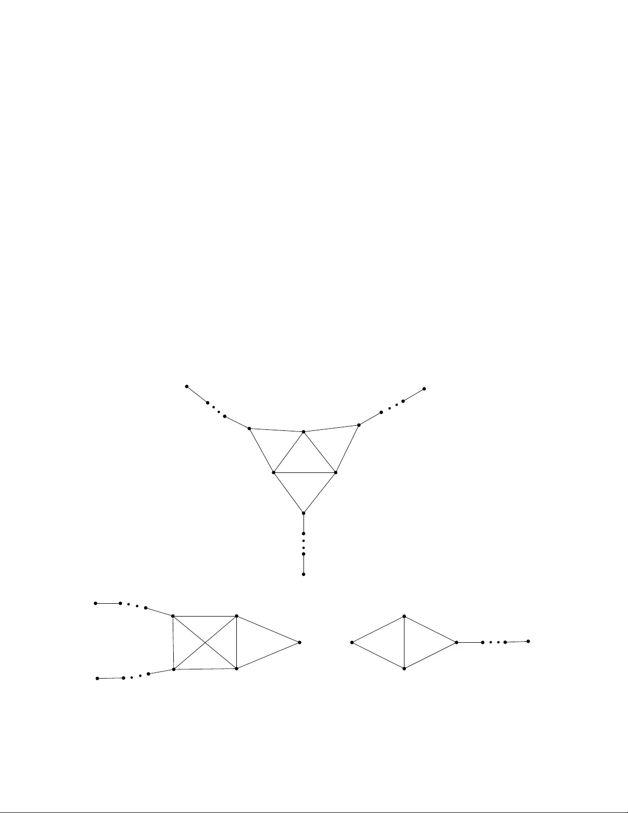
CLASSIFICA TION OF UNMIXED P ARITY BINOMIAL EDGE IDEALS OF CA CTUS AND CHORD AL GRAPHS DEBLINA DEY, A. V. JA Y ANTHAN, AND SARANG SANE Abstract. In this article, w e characterize all unmixed and Cohen-Macaula y parity binomial edge ideals of cactus and c hordal graphs in terms of the structural prop erties of the graph. 1. Introduction Let G b e a finite simple graph on the vertex set V ( G ) = [ n ] = { 1 , . . . , n } and the edge set E ( G ). Kahle, Sarmien to and Windisch in 2016, [9], introduced p arity binomial e dge ide als : I G := ( x i x j − y i y j : { i, j } ∈ E ( G )) ⊂ R = K [ x 1 , . . . , x n , y 1 , . . . , y n ] , where K is a field. This ideal is a subtle v ariation of another class of binomial ideals, called binomial e dge ide al , defined by Herzog et al., [8]: J G := ( x i y j − x j y i : { i, j } ∈ E ( G )) ⊂ R = K [ x 1 , . . . , x n , y 1 , . . . , y n ] , A close relation has b een observed b etw een several algebraic prop erties and/or inv arian ts of these edge ideals and combinatorial prop erties and/or inv ariants of the graph G . If G is a bipartite graph, then its parity binomial edge ideal is obtained from its binomial edge ideal b y a simple change of v ariables. As noted in the pap er of Kahle et al., parit y binomial edge ideals share a n umber of prop erties with binomial edge ideals, but the combinatorics is subtler. In [9], the authors describ ed a Gr¨ obner basis for I G . If c har( K )  = 2, they show that I G is a radical ideal and explicitly obtain the structure of the minimal primes in terms of the disconnector sets (see Definition 2.3) of the graph. Our study of the unmixed property of I G crucially uses this description of the minimal primes and hence in this article, w e assume that char( K )  = 2. In [12], Kumar studied some of the structural prop erties of I G . He prov ed that for a bipartite graph G , I G is a complete intersection if and only if G is a disjoint union of paths, and, for a non-bipartite graph, I G is a complete intersection if and only if G is a cycle on an odd num ber of v ertices. He also classifies graphs with almost complete in tersection parity binomial edge ideals and establishes when their asso ciated Rees algebra R ( I G ) is Cohen-Macaulay . Among the homological inv arian ts, Betti num bers, Casteln uo v o-Mumford regularit y and depth are w ell studied for many classes of homogeneous ideals of p olynomial rings. While computation of depth is in general challenging, one particular instance, of maximal depth, i.e., b eing Cohen- Macaula y , has received a lot of atten tion. An ideal I in a No etherian ring R is said to b e Cohen-Macaula y if R/I is Cohen-Macaula y . Understanding the Cohen-Macaulayness of an ideal is a classical topic. When it comes to ideals as- so ciated with certain geometric/topological/combinatorial structures, the attempt is to c haracterize the Cohen-Macaula yness in terms of the structure asso ciated with the ideal. When G is a bipartite graph, Bolognini, Macchia and Strazzanti completely characterized when the binomial edge ideal J G (and hence the parit y binomial edge ideal I G ) is Cohen-Macaula y in terms of the structure of G , [1]. F or an arbitrary graph G , Bolognini et al. conjectured that J G is Cohen-Macaulay if and only if G is accessible (see [2] for the details). They pro v ed the ‘only if ’ part of this conjecture and 2020 Mathematics Subje ct Classific ation. Primary 05E40; Secondary 13C13, 13C14. Key wor ds and phrases. Chordal graphs, disconnector sets, parit y binomial edge ideals, unmixedness, Cohen- Macaula yness. 1 2 DEBLINA DEY, A. V. JA Y ANTHAN, AND SARANG SANE pro v ed the ‘if ’ part for c hordal graphs and graphs con taining a Hamiltonian path. The general case is still open. F or the case of parity binomial edge ideals, no suc h results, and not ev en a conjecture is a v ailable in this direction. An y Cohen-Macaulay ideal must b e unmixed. Hence, to understand the Cohen-Macaulayness, one should understand the unmixed prop ert y of the ideal as well. In this article, we first inv estigate the unmixedness of parity binomial edge ideals of non-bipartite c hordal graphs. As a consequence of our inv estigation, w e are also able to characterize their Cohen-Macaulayness as w ell. The unmixed prop ert y of the parity binomial edge ideal is muc h more complex than that of the binomial edge ideals. In the case of binomial edge ideals, the combinatorial ob ject that determines the minimalit y of an asso ciated prime is called a cut set and there is a unique prime ideal asso ciated to each cut set. In the case of parity binomial edge ideals, the corresp onding ob ject is called a disconnector set and there are several prime ideals asso ciated with one disconnector set. Our inv es- tigation of the unmixedness prop ert y crucially dep ends on the construction of suitable disconnector sets. W e briefly describ e the structure of the article. After discussing preliminaries in Section 2, we study the unnmixedness of parit y binomial edge ideals of cactus graphs in Section 3. W e prov e that for a connected non-bipartite cactus graph G , I G is unmixed only if it is Cohen-Macaulay if and only if it is Gorenstein if and only if it is a complete intersection if and only if G is an o dd cycle, Theorem 3.10. P 1 P 2 P 3 Class G 1 α 1 α 2 α 3 β 1 β 2 β 3 P 1 P 2 P 3 α 1 α 2 α 1 α 2 x 2 x 1 x 1 y 1 x 2 Class G 2 Class G 3 Figure 1. Unmixed c hordal graph classes: G 1 , G 2 and G 3 , where P 1 , P 2 , P 3 are path graphs of length at least one CLASSIFICA TION OF UNMIXED P ARITY BINOMIAL EDGE IDEALS OF CACTUS AND CHORDAL GRAPHS 3 A chordal graph can b e realized as a clique sum of complete graphs (immediate consequence of [15, Theorem 5.3.17]). W e use this structure to describ e some disconnector sets which we further use for classifying when the parit y binomial edge ideals are unmixed. deleted ” Let G b e the clique sum of K n 1 , K n 2 , . . . , K n t . F or j ≥ 2, w e define K r j = ( ∪ i c G ( S \ { s } ) for every s ∈ S . A vertex s ∈ V ( G ) is said to b e a cut vertex if { s } is a cut set of G . A blo ck of a graph is a maximal connected induced subgraph that has no cut v ertex. F or example the blo c ks of a cactus graph are cycles or edges. Definition 2.3. [9, Definition 4.5] A set S ⊆ V ( G ) is a disc onne ctor of G if b G ( S ) + c G ( S ) > b G ( S \ { s } ) + c G ( S \ { s } ) for every s ∈ S . The empty set is always a disc onne ctor of any gr aph. F or a graph G on [ n ], let J G := I G : ( Q i ∈ V ( G ) x i y i ) ∞ ⊂ K [ x 1 , . . . , x n , y 1 , . . . , y n ] . Throughout this article, w e will assume that char( K )  = 2. F or a graph G with an o dd cycle, let p + ( G ) := ( x i + y i : i ∈ V ( G )) and p − ( G ) := ( x i − y i : i ∈ V ( G )). Let G b e a graph with bipartite connected comp onents B 1 , . . . , B r and non-bipartite connected comp onen ts N 1 , . . . , N t . In [9], it is pro v ed that the minimal primes of J G are of the form P r i =1 J B i + P t i =1 p σ i ( N i ), where σ i ∈ { + , −} . Let S ⊂ V ( G ) b e a disconnector of G . Let q = P r i =1 J B ′ i + P t i =1 p σ i ( N ′ i ) b e a minimal prime of J G \ S . Then q is sign-split if for all s ∈ S such that C G \ S ( s ) c on tains no bipartite graphs, the prime summands of q corresp onding to connected components in C G \ S ( s ) are not all equal to p + or not all equal to p − . Not every disconnector set of a graph admits a sign-split minimal prime of J G , see [9, Example 4.14]. F or S ⊂ [ n ], let m S = ( x i , y i : i ∈ S ). Kahle et al. pro v ed that the minimal primes of I G are ideals m S + p , where S ⊂ V ( G ) is a disconnector set of G and p is a sign-split minimal prime of J G \ S , see [9, Theorem 4.15]. Notation 2.4. A disconnector set S ⊆ V ( G ) is said to b e a sign split disconnector set if J G \ S has a minimal prime, that satisfies the sign-split prop erty. W e denote the collection of all sign-split disconnector sets of G by D ( G ). Definition 2.5. The ide al I ⊆ R is said to b e unmixe d if al l its asso ciate d primes have the same height. If char ( K )  = 2, then I G is radical. So, in this case I G has same set of asso ciated and minimal primes. The heigh t of the minimal primes of I G are giv en in [12]. Let Q σ S ( G ) = m S + q b e a minimal prime of I G . Then, heigh t Q σ S ( G ) = | S | + n − b G ( S ). Therefore, I G is unmixed if and only if b G ( S ) = | S | + b ( G ) for all S ∈ D ( G ). 2.1. Disconnector sets and unmixedness. While a disconnector set may not alwa ys satisfy the sign-split prop ert y , some restriction on the set allows it to b e sign-split as discussed b elo w. R emark 2.6 . [9, Remark 4.12] Let S b e a disconnector set of G such that every v ertex of S is connected with some bipartite connected comp onen t of G \ S . Then S satisfies the sign-split prop ert y trivially . CLASSIFICA TION OF UNMIXED P ARITY BINOMIAL EDGE IDEALS OF CACTUS AND CHORDAL GRAPHS 5 Prop osition 2.7. L et S b e a disc onne ctor set of G such that every element of S is adjac ent to vertic es of a fixe d non-bip artite c onne cte d c omp onent of G \ S . Then S satisfies the sign-split pr op erty. Pr o of. Let Q b e the non-bipartite connected comp onen t of G \ S such that C G \ S ( s ) ∋ Q for all s ∈ S . Then corresp onding to Q , we c ho ose p + ( Q ) and for any other non-bipartite connected comp onen t Q ′ of G \ S , we take p − ( Q ′ ). Hence, the sign-split prop ert y is preserved. □ F or a non-bipartite graph G , I G is unmixed if and only if | S | = b G ( S ) for all S ∈ D ( G ). The follo wing result prop oses a necessary condition on S so that it satisfies the ab ov e equalit y . Prop osition 2.8. L et G b e a non-bip artite gr aph and S ∈ D ( G ) . If ther e exists T ⊆ S , such that I G \ T is unmixe d and G \ T has exactly | T | bip artite c omp onents ( b ( G \ T ) = | T | ) , then | S | = b G ( S ) . Pr o of. Since S ∈ D ( G ), S \ T ∈ D ( G \ T ) and b G ( S ) = b ( G \ T ) ( S \ T ). Since I G \ T is unmixed, | S \ T | = b ( G \ T ) ( S \ T ) + b ( G \ T ). F rom the given hypothesis, b ( G \ T ) = | T | . So, | S \ T | = b G ( S ) + | T | = ⇒ | S | = b G ( S ). □ The follo wing remark shows that the study of the unmixed and Cohen-Macaulay prop erties of I G can b e reduced to the case of connected graphs. R emark 2.9 . Let G = G 1 ⊔ G 2 ⊔ · · · ⊔ G m b e a graph, where G i are the connected comp onents. (i) By definition it follows that D ( G ) = { S 1 ∪ S 2 ∪ · · · ∪ S m : S i ∈ D ( G i ) } . (ii) By (i), it follows that I G is unmixed if and only if I G i is unmixed for all 1 ≤ i ≤ m . (iii) Note that R I G ≡ R 1 I G 1 ⊗ K R 2 I G 2 ⊗ K · · · ⊗ K R m I G m , where R i = K [ x j , y j : j ∈ V ( G i )]. Therefore I G is Cohen-Macaulay if and only if I G i is Cohen-Macaulay for each 1 ≤ i ≤ m [3, Theorem 2.1]. F or the rest of the article, G denotes a connected simple graph unless stated otherwise. 3. Cohen-Maca ula y p arity binomial edge ideal of cactus graphs W e study the parity binomial edge ideals of cactus graphs in this section. The classification of Cohen-Macaulay parity binomial edge ideals asso ciated with bipartite cactus graphs are known from the work of Rinaldo [14]. So, we assume that our graphs are non-bipartite cactus graphs. The parit y binomial edge ideal of an o dd cycle is a complete intersection and hence Cohen-Macaulay [12, Theorem 3.5]. W e pro ve that these are the only Cohen-Macaulay cases among the connected non-bipartite cactus graphs. First of all, we observe that given any tw o vertices in a cactus graph G , there is some kind of uniqueness in the path joining these tw o v ertices. Let G b e a cactus graph and u, v ∈ V ( G ). F or an y path P from u to v , let C P = { C : C is a cycle in G suc h that C ∩ P is an edge in G } . Then, the set C P is indep endent of the path P . Supp ose there are tw o distinct paths P 1 and P 2 from u to v such that C P 1  = C P 2 . If V ( P 1 ) ∩ V ( P 2 ) = { u = x 0 , x 1 , . . . , x r − 1 , x r = v } , then there exists an i ∈ { 0 , . . . , r − 1 } such that for the part P ij of P j , j = 1 , 2, joining x i and x i +1 , C P i 1  = C P i 2 . Now consider the induced subgraph on V ( P i 1 ) ∪ V ( P i 2 ) ∪ ( ∪ C ∈C P i 1 ∪C P i 2 V ( C )) is a blo ck in G which is neither an edge, nor a cycle. This contradicts the assumption that G is a cactus. Therefore, giv en an y tw o cycles C and C ′ of G , there exist t wo unique v ertices u ∈ V ( C ) and u ′ ∈ V ( C ′ ) such that an y path connecting C and C ′ alw a ys passes through b oth u and u ′ . W e say that u and u ′ are the connecting v ertices of C and C ′ in G . Definition 3.1. An o dd cycle C of a gr aph G is said to b e p endant if ther e exists v ∈ V ( C ) so that any p ath in G fr om a vertex of C to any vertex of an o dd cycle in G \ { v } always p asses thr ough v . We denote such a p endant o dd cycle by ( C, v ) . 6 DEBLINA DEY, A. V. JA Y ANTHAN, AND SARANG SANE C 1 C 2 C 3 v 1 v 3 Figure 2. A cactus graph. Note that ( C 1 , v 1 ) and ( C 3 , v 3 ) are p endant o dd cycles of G but C 2 is not. R emark 3.2 . Note that the ab ov e definition is similar to, but not quite the same as the standard notion of p endan t vertex in graph theory . F or example in the ab ov e Figure 2, there can b e ev en cycles or edges attac hed to the vertices of C 1 or C 3 , but they still satisfy the definition of p endan t o dd cycles. It follows from the definition of a p endan t o dd cycle that if G has a unique o dd cycle, then it is p endant. Supp ose there is more than one o dd cycle. Recall from the ab o v e discussion that any o dd cycle C is connected to another o dd cycle C ′ through a unique vertex v ∈ V ( C ). Define ϵ ( C ) to b e the num b er of distinct vertices in V ( C ) that connect C with other o dd cycles of G . Then C is a p endan t o dd cycle if and only if ϵ ( C ) = 1. It follows from the structure of cactus graphs that a p endant o dd cycle alwa ys exists. W e giv e a pro of b elo w. Prop osition 3.3. L et G b e a c actus gr aph with at le ast two o dd cycles. Then G has a p endant o dd cycle. Pr o of. W e assume that G is connected. Let C and C ′ b e t wo different o dd cycles in G , and u ∈ V ( C ) and u ′ ∈ V ( C ′ ) b e the connecting vertices. Let us define δ ( u, u ′ ) = min { n ( P ) : P is a path b etw een u and u ′ } , where n ( P ) is n um b er of distinct odd cycles in G intersecting the path P . Consider the set { δ ( u, u ′ ) } o v er all pairs of odd cycles and connecting vertices u ∈ V ( C ) and u ′ ∈ V ( C ′ ). Supp ose the maxim um is ac hiev ed for the v ertices v 1 ∈ V ( C 1 ) and v 2 ∈ V ( C 2 ). Claim: ( C 1 , v 1 ) is a p endant o dd cycle. Pro of: Supp ose it is not. Then there exists another o dd cycle C 3  = C 1 , C 2 , v 1  = v ′ 1 ∈ V ( C 1 ) and v 3 ∈ V ( C 3 ) such that C 1 and C 3 are connected through v ′ 1 and v 3 . Therefore, there is a path connecting v 3 in C 3 and v 2 in C 2 passing through v ′ 1 in C 1 . Since G is a cactus graph, an y path from C 3 to C 2 passes through C 1 . So, an y path from v 3 to v 2 passes through v ′ 1 and v 1 . Since C 3 in tersects any path from v 3 to v 2 and it do es not in tersect an y path from v 1 to v 2 , we get δ ( v 2 , v 3 ) ≥ δ ( v 2 , v 1 ) + 1 > δ ( v 2 , v 1 ). This is a con tradiction to the selection of v 1 and v 2 . Hence ( C 1 , v 1 ) is a p endant o dd cycle. □ Notation 3.4. Let G b e a cactus graph and ( C , v ) b e a p endant o dd cycle of G . Note that v is a cut vertex and { v } ∈ D ( G ). It follows that C \ { v } must be con tained in a bipartite connected comp onen t of G \ { v } , say G 0 . W rite G \ { v } = G 0 ⊔ G ′ . Here G ′ is the union of connected comp onen ts of G \ { v } except G 0 . Our aim is to sho w that unmixedness descends from I G to I G ′ . F or this purp ose, we first prov e a couple of technical lemmas. Lemma 3.5. With the notation as in The or em 3.4, let S ⊆ V ( G ′ ) . Then c G ( S ∪ { v } ) = c G ′ ( S ) + 1 and b G ( S ∪ { v } ) = b G ′ ( S ) + 1 . CLASSIFICA TION OF UNMIXED P ARITY BINOMIAL EDGE IDEALS OF CACTUS AND CHORDAL GRAPHS 7 Pr o of. Since G \ { v } = G 0 ⊔ G ′ and S ⊆ V ( G ′ ), w e ha v e C G ( S ∪ { v } ) = C G \{ v } ( S ) = C G 0 ⊔ G ′ ( S ) = C G ′ ( S ) ⊔ { G 0 } . Similarly , B G ( S ∪ { v } ) = B G ′ ( S ) ⊔ { G 0 } . Hence the assertion follo ws. □ Lemma 3.6. With the notation as in The or em 3.4, if S ∈ D ( G ′ ) , then S ∪ { v } ∈ D ( G ) . Pr o of. Let S ∈ D ( G ′ ). Therefore S is a sign-split disconnector set of G ′ and for ev ery s ∈ S , c G ′ ( S ) + b G ′ ( S ) > c G ′ ( S \ { s } ) + b G ′ ( S \ { s } ). Then it follows from Theorem 3.5 that for every s ∈ S, c G ( S ∪ { v } ) + b G ( S ∪ { v } ) > c G (( S ∪ { v } ) \ { s } ) + b G (( S ∪ { v } ) \ { s } ) . Since G 0 is bipartite and G is non-bipartite, c G ( S ∪ { v } ) + b G ( S ∪ { v } ) > c G ( S ) + b G ( S ). W e now pro v e that S ∪ { v } satisfies the sign-split prop erty . Note that S has a sign-split prop erty in G ′ . Let s ∈ S ∪ { v } . If s  = v , then C G \ ( S ∪{ v } ) ( s ) = C G ′ \ S ( s ). If s = v , then C G \ ( S ∪{ v } ) ( s ) = C G ′ \ S ( s ) ∪ { G 0 } , and G 0 is bipartite. Hence in b oth cases S ∪ { v } satisfies sign-split prop erty in G . Therefore S ∪ { v } ∈ D ( G ). □ W e now prov e that the unmixedness prop ert y descends. Prop osition 3.7. With the notation as in The or em 3.4, if I G is unmixe d, then so is I G ′ . Pr o of. Since { v } ∈ D ( G ) and I G is unmixed, b G ( { v } ) = 1. Hence the connected comp onents of G \ { v } other than G 0 m ust b e non-bipartite. In particular, G ′ m ust b e non-bipartite. It follows from Theorem 3.6 that for all S ∈ D ( G ′ ), S ∪ { v } ∈ D ( G ). As I G is unmixed, b G ( S ∪ { v } ) = | S ∪ { v }| . This implies b G ′ ( S ) = | S | , by Theorem 3.5. Thus I G ′ is unmixed. □ W e now pro ceed to c haracterize the cactus graphs having unmixed parity binomial edge ideals. Prop osition 3.8. L et G b e a non-bip artite c actus gr aph with only one o dd cycle. Then I G is unmixe d if and only if G is an o dd cycle. Pr o of. The ‘if part’ follows from [12, Theorem 3.5]. Now assume that I G is unmixed. Let C b e the o dd cycle in G . If there exists a v ∈ V ( C ) such that deg G ( v ) > 2, then v is a cut vertex. Th us { v } ∈ D ( G ). Moreov er, G \ { v } is bipartite and has at least tw o components, i.e., b G ( { v } ) ≥ 2. This con tradicts the unmixedness of I G . Hence for every v ∈ V ( C ), deg G ( v ) = 2. Therefore, G = C . □ W e no w sho w that if a cactus graph contains more than one o dd cycle, then the parit y binomial edge ideal is not unmixed. Theorem 3.9. L et G b e a c actus gr aph having at le ast two o dd cycles as sub gr aphs, then I G is not unmixe d. Pr o of. W e prov e the statement b y induction on r ( G ), the num ber of o dd cycles in G . First assume that r ( G ) = 2 and I G is unmixed. Since G is cactus with only tw o o dd cycles, b oth must b e p endan t o dd cycles, say ( C 1 , v 1 ) and ( C 2 , v 2 ). If v 1 = v 2 , then { v 1 } ∈ D ( G ) and b G ( { v 1 } ) = 2 which is a con tradiction to the unmixedness of I G . Supp ose v 1  = v 2 . First, we take the disconnector set { v 1 } . Supp ose G \ { v 1 } = G 0 ⊔ G ′ , where G 0 is the bipartite comp onent con taining C 1 \ { v 1 } and G ′ is the non-bipartite graph containing C 2 . Since b G ( { v 1 } ) = 1 and since there are only t w o odd cycles in G , G ′ is also connected. Moreo v er, Theorem 3.7 implies that I G ′ is unmixed. But G ′ is a connected cactus graph with only one o dd cycle. So, from Theorem 3.8, it follows that G ′ is an o dd cycle, i.e., G ′ = C 2 . Using the same argumen t for { v 2 } , w e get G \ { v 2 } = ( C 2 \ { v 2 } ) ⊔ C 1 . So, V ( G ) = V ( C 1 ) ∪ V ( C 2 ) and E ( G ) = E ( C 1 ) ∪ E ( C 2 ) ∪ { e } , where e = { v 1 , v 2 } is the only edge b et w een C 1 and C 2 . Cho ose x 1 ∈ V ( C 1 ) \ { v 1 } and x 2 ∈ V ( C 2 ) \ { v 2 } . Then { x 1 , x 2 } ∈ D ( G ), but b G ( { x 1 , x 2 } ) = 1, a contradiction to the unmixedness of I G . Therefore I G is not unmixed. No w let r ( G ) ≥ 3 and assume by induction that if H is a connected non-bipartite cactus graph with 2 ≤ r ( H ) < r ( G ), then I H is not unmixed. Supp ose I G is unmixed. Let ( C , v ) b e a pendant 8 DEBLINA DEY, A. V. JA Y ANTHAN, AND SARANG SANE o dd cycle of G . Then { v } ∈ D ( G ) . If v is contained in more than one p endant o dd cycles, then b G ( { v } ) > 1 which contradicts the unmixedness of I G . Thus w e can write G \ { v } = G 0 ⊔ G ′ , where G 0 is the bipartite comp onent containing C \ { v } and G ′ is a non-bipartite graph with each comp onen t a non-bipartite cactus graph. Observe that G ′ will not hav e any bipartite comp onent, since otherwise b G ( { v } ) > 1 contradicting the unmixedness of I G . Note that for an y non-bipartite connected comp onent H of G ′ , r ( H ) < r ( G ). W e know from Theorem 3.7 that I G ′ is unmixed. No w w e ha ve t wo cases. Case 1: If an y of the connected comp onen ts of G ′ has at least t wo o dd cycles, then b y induction h yp othesis I G ′ is not unmixed, which contradicts Theorem 3.7. Case 2: Supp ose every non-bipartite connected comp onent of G ′ has only one o dd cycle. Since I G is unmixed, so is I G ′ , by Theorem 3.7. Therefore, by Theorem 3.8, we get that all these connected comp onen ts of G ′ are cycles. W rite G ′ = C 1 ⊔ C 2 ⊔ · · · ⊔ C k , where C i are o dd cycles. Let v i ∈ V ( C i ) b e such that { v , v i } ∈ E ( G ). Since G is a cactus graph, these v i are the unique vertices of C i that are adjacen t to v . Hence ( C i , v i ) are all p endant o dd cycles of G , for 1 ≤ i ≤ k . No w consider G \ { v 1 } = G ′ 0 ⊔ G ′′ , where G ′ 0 is the bipartite comp onent containing C 1 \ { v 1 } and G ′′ is the non-bipartite connected comp onent containing C , C 2 , . . . , C k . Since r ( G ) ≥ 3, k ≥ 2. Hence by induction I G ′′ is not unmixed. But this con tradicts the conclusion b y Theorem 3.7 that I G ′′ is unmixed. Hence I G is not unmixed. □ Summarizing all the ab ov e results, we get: Corollary 3.10. L et G b e a non-bip artite c actus gr aph. Then the fol lowing ar e e quivalent: (1) I G is unmixe d; (2) I G is Cohen-Mac aulay; (3) I G is Gor enstein; (4) I G is a c omplete interse ction; (5) G is an o dd cycle. Pr o of. The implications (4) ⇒ (3) ⇒ (2) ⇒ (1) are alwa ys true. By [12], (4) and (5) are equiv alen t. The implication (1) ⇒ (5) follows from Theorem 3.8 and Theorem 3.9. □ 4. The algorithm Unlik e cactus graphs, it is not clear how to study the unmixed prop erty of I G using hereditary b eha vior for chordal graphs. T o understand the unmixed prop erty , we first prop ose an algorithm for chordal graphs to construct a maximal induced tree H n along with a disconnector set S n ( G ). W e show that if I G is unmixed, then these trees are alwa ys path graphs. Notation 4.1. Let G b e a c hordal graph which is a clique sum of K n 1 , . . . , K n t . W e define K r j = ( ∪ i 0 } , M (Γ 0 1 ) = { maximal elemen ts of Γ 0 1 with resp ect to the order relation ⊆} . Fix L 0 1 ∈ M (Γ 0 1 ) . Outputs of iter ation 1 : L 0 1 . Pr o c e e d to Iter ation 2 in Step 0 . Iter ation q ≥ 2 : Inputs: L 0 i , i < q . Define T 0 q = T 0 q − 1 \ L 0 q − 1 = [ t ] \  q − 1 [ j =1 L 0 j  , Γ 0 q = { L ⊆ [ t ] : L ∩ T 0 q  = ∅ , m ( L ) > 0 } , M (Γ 0 q ) = { maximal elemen ts of Γ 0 q with resp ect to the order relation ⊆} , M 1 (Γ 0 q ) = { L ∈ M (Γ 0 q ) : L ∩ L 0 i  = ∅ for exactly one i < q } , If M 1 (Γ 0 q ) = ∅ , then the 0 th step terminates . Else M 2 (Γ 0 q ) = { L ∈ M 1 (Γ 0 q ) : | L ∩ L 0 i | is minimum } . Cho ose L 0 q ∈ M 2 (Γ 0 q ) and x 0 q ∈ \ i ∈ L 0 q V ( K n i ). Outputs of Iter ation q : L 0 q . Pr o c e e d to Iter ation q + 1 in Step 0 . CLASSIFICA TION OF UNMIXED P ARITY BINOMIAL EDGE IDEALS OF CACTUS AND CHORDAL GRAPHS 11 Once the 0 th step terminates, define D 0 = { 1 } ∪ { q : M 1 (Γ 0 q )  = ∅} and H 0 = G [ { x 0 q : q ∈ D 0 } ] . A 0 2 = { i ∈ [ t ] : i ∈ ( L 0 q 1 ∩ L 0 q 2 ) for q 1  = q 2 ∈ D 0 } , A 0 1 = { i ∈ [ t ] : i ∈ L 0 q for exactly one q ∈ D 0 } , A 0 0 = { i ∈ [ t ] : i / ∈ L 0 q for all q } . Outputs of Step 0 : A 0 2 , A 0 1 , A 0 0 , H 0 , D 0 . Pro ceed to Step 1. Step p for p ≥ 1 : Inputs: A p − 1 0 , A p − 1 1 , A p − 1 2 . Define T p 0 = A p − 1 1 ∪ A p − 1 0 , L p 0 = ∅ , Iter ation q , q ≥ 1 : Inputs: L p i , i < q . Define T p q = T p q − 1 \ L p q − 1 Γ p q = { L ⊆ T p q : L ∩ A p − 1 1  = 0 and \ i ∈ L V ( K n i ) \ [ j ∈ A p − 1 2 ∪ q − 1 s =0 L p s V ( K n j )  = ∅} . If Γ p q = ∅ , then the p th step terminates . Else M (Γ p q ) = { maximal elemen ts of Γ p q with resp ect to the order relation ⊆} , Cho ose L p q ∈ M (Γ p q ) and x p q ∈ \ i ∈ L p q V ( K n i ) \ [ j ∈ A p − 1 2 ∪ q − 1 s =0 L p s V ( K n j ). Outputs of Iter ation q : L p q . Pr o c e e d to Iter ation q + 1 in Step p . Once the p th step terminates, define D p = { q : M (Γ p q )  = ∅} and H p = G [ { x i q : i ∈ [ p ] , q ∈ ∪ j ∈ [ p ] D j } ] . A p 2 = A p − 1 2 ∪ A p − 1 1 , A p 1 = { i ∈ A p − 1 0 : i ∈ L p q for some q ∈ D p } , A p 0 = [ t ] \ ( A p 2 ∪ A p 1 ) . Outputs of Step p : A p 2 , A p 1 , A p 0 , D p , H p . If A p 1 = ∅ , then the algorithm terminates. Else pro ceed to Step p + 1. R emark 4.7 . (1) Note that the sets A p 0 , A p 1 , A p 2 , the graphs H p , and the num ber of steps of the algorithm will v ary dep ending on the choices of L p q and x p q . Let L b e the collection of all data in one run of the algorithm with fixed c hoices of L p q , which we denote by L p q ( L ), and n( L ) denote the last step of the algorithm for these fixed choices. Sp ecifically L represen ts one run of iteration of the algorithm. If L is fixed, then we use n instead of n( L ) and L p q instead of L p q ( L ). (2) Observe that A p 0 ⊔ A p 1 = A p − 1 0 and A p 2 , A p 1 and A p 0 is a partition of [ t ]. (3) At each step of the algorithm we construct a subgraph H p of G and for p < p ′ , H p is a subgraph of H p ′ . 12 DEBLINA DEY, A. V. JA Y ANTHAN, AND SARANG SANE K n 4 K n 3 K n 2 K n 1 1 2 3 4 5 6 7 Figure 3. The smallest graph G in the class G 2 Example 4.8. Let G b e the clique sum of K n 1 , K n 2 , K n 3 and K n 4 as sho wn in Figure 3. Step 0 : Iteration 1: T 0 1 = { 1 , 2 , 3 , 4 } , So, Γ 0 1 = {{ 1 } , { 2 } , { 3 } , { 4 } , { 1 , 2 } , { 2 , 3 } , { 2 , 4 }} . This im- plies M (Γ 0 1 ) = {{ 1 , 2 } , { 2 , 3 } , { 2 , 4 }} . Cho ose L 0 1 = { 1 , 2 } ∈ M (Γ 0 1 ) and x 0 1 = 2 ∈ V ( K n 1 ) ∩ V ( K n 2 ). Outputs of Iter ation 1: L 0 1 = { 1 , 2 } . Iteration 2: Inputs: L 0 1 . T 0 2 = T 0 1 \ L 0 1 = { 3 , 4 } . So, Γ 0 2 = {{ 3 } , { 4 } , { 2 , 3 } , { 2 , 4 } and M (Γ 0 2 ) = {{ 2 , 3 } , { 2 , 4 }} . Therefore, M 1 (Γ 0 q ) = {{ 2 , 3 } , { 2 , 4 }} . W e Cho ose L 0 2 = { 2 , 3 } and x 0 2 = 4 ∈ V ( K n 2 ) ∩ V ( K n 3 ). Outputs of Iter ation 2: L 0 2 = { 2 , 3 } . Iteration 3: Inputs: L 0 1 , L 0 2 . T 0 3 = T 0 2 \ L 0 2 = { 4 } and M (Γ 0 3 ) = {{ 2 , 4 }} but M 1 (Γ 0 3 ) = ∅ . So, Step 0 terminates. Outputs of Step 0 : D 0 = { 1 , 2 } , H 0 = G [ { x 0 q : q ∈ D 0 } ] = G [ { 2 , 4 } ]. A 0 2 = { 2 } , A 0 1 = { 1 , 3 } and A 0 0 = { 4 } , K n 4 K n 3 K n 2 K n 1 2 4 Figure 4. Step 0: H 0 Step 1 : Inputs: A 0 2 , A 0 1 , A 0 0 . Iteration 1: T 1 1 = A 0 1 ∪ A 0 0 = { 1 , 3 , 4 } . Then Γ 1 1 = M (Γ 1 1 ) = {{ 1 } , { 3 }} . Cho ose L 1 1 = { 1 } and x 1 1 = 1 ∈ V ( K n 1 ) \ V ( K n 2 ). Outputs of Iter ation 1: L 1 1 = { 1 } Iteration 2: Inputs: L 1 1 . T 1 2 = T 1 1 \ L 1 1 = { 3 , 4 } . Then Γ 1 2 = M (Γ 1 2 ) = {{ 3 }} . CLASSIFICA TION OF UNMIXED P ARITY BINOMIAL EDGE IDEALS OF CACTUS AND CHORDAL GRAPHS 13 Cho ose L 1 2 = { 3 } and x 1 2 = 6. Outputs of Iter ation 2: L 1 2 = { 3 } Iteration 3: Inputs: L 1 1 , L 1 2 . T 1 3 = T 1 2 \ L 1 2 = { 4 } . Since T 1 3 ∩ A 0 1 = ∅ , Γ 1 3 = ∅ . Hence, the Step 1 terminates. Outputs of Step 1 : D 1 = { 1 , 2 } and the induced subgraph H 1 = G [ x 0 1 , x 0 2 , x 1 1 , x 1 2 ] = G [ { 2 , 4 , 1 , 6 } ]. A 1 2 = A 0 2 ∪ A 0 1 = { 1 , 2 , 3 } , A 1 1 = ∅ and A 1 0 = { 4 } . K n 4 K n 3 K n 2 K n 1 2 4 6 1 Figure 5. Step 1: H 1 Since A 1 1 = ∅ , the algorithm terminates after Step 1. Note that the induced induced subgraph H 1 is a maximal tree of G . Let us construct the set S = ( ∪ i ∈ A 1 2 V ( K n i )) \ V ( H 1 ) = { 3 , 5 } . then S is a sign-split disconnector set of G and H 1 is a comp onent of G \ S . Lemma 4.9. The algorithm describ e d ab ove terminates after a finite numb er of steps. Pr o of. Since A p 0 ⊔ A p 1 = A p − 1 0 , it follows that A p 1 = ∅ if and only if A p 0 = A p − 1 0 . Hence, the algorithm terminates if A p − 1 0 = A p 0 . Since  A p 0  p ≥ 1 is a strictly descending c hain of subsets of [ t ], this implies that the algorithm must terminate in at most t + 1 steps. □ No w we prov e t wo lemmas that giv e some detailed information ab out certain outcomes of the algorithm. The proof essen tially follo ws from our construction of the sets Γ p q in the algorithm. These t w o results are useful in understanding disconnector sets. Lemma 4.10. F or p ≥ 1 , if i ∈ A p − 1 1 , then either i ∈ L p q for some q ∈ D p or V ( K n i ) ⊆ [ j ∈ A p − 1 2 ∪ q ∈ D p L p q V ( K n j ) . Pr o of. F rom the algorithm, it follo ws that L p q ∩ A p − 1 1  = ∅ . So, either i ∈ L p q for some q ∈ D p or i / ∈ ∪ q ∈ D p L p q . Supp ose s is the highest index in D p , i.e., Γ p s +1 = ∅ . Note that Γ p s +1 = { L ⊆ T p s +1 : L ∩ A p − 1 1  = 0 and \ i ∈ L V ( K n i ) \ [ j ∈ A p − 1 2 ∪ s j =1 L p j V ( K n j )  = ∅} . No w, if i / ∈ L p q for all q ∈ D p , then tak e the set L = { i } . Clearly L ∩ A p − 1 1  = ∅ and L ⊆ T p s +1 . Since Γ p s +1 = ∅ , V ( K n i ) should b e contained in S j ∈ A p − 1 2 ∪ q ∈ D p L p q V ( K n j ). □ R emark 4.11 . If the algorithm terminates after the nth step, then there are tw o p ossibilities. (1) either Γ n 1 = ∅ , i.e., for any i ∈ A n − 1 1 , V ( K n i ) ⊆ S j ∈ A n − 1 2 V ( K n j ). (2) or for any i ∈ L n q , i / ∈ A n − 1 0 . 14 DEBLINA DEY, A. V. JA Y ANTHAN, AND SARANG SANE Observ e that the iteration at the 0th step is differen t from the iterations at p th step for p ≥ 1. In fact, for p ≥ 1, there is rep etition in the algorithm. W e notice that irresp ective of our choices, the sets L 0 q satisfy some combinatorial prop erties. W e first prov e them. Later, using those prop erties, w e show that H 0 is a tree. F urthermore, w e establish that H p is a tree for all p and for any choices of L p q . Notation 4.12. F or any set L ⊆ [ t ], µ ( L ) denotes the minimum element of the set L . Lemma 4.13. F or every i ∈ L 0 q , if i  = µ ( L 0 q ) , then λ ( i ) ⊆ L 0 q . Pr o of. Since i  = µ ( L 0 q ), i > µ ( L 0 q ). So, from Theorem 4.3, K n µ ( L 0 q ) ∩ K n i = K n µ ( L 0 q ) ∩ ( K n i ∩ l ∈ λ ( i ) K n l ). This implies that m ( L 0 q ) = m ( L 0 q ∪ λ ( i )). Since L 0 q is a maximal element of Γ 0 q , λ ( i ) ⊆ L 0 q . □ Example 4.14. In Figure 3, λ (2) = { 1 } and λ (3) = { 2 } . Note that λ (2) ⊂ L 0 1 and λ (3) ⊂ L 0 2 . Lemma 4.15. L et i ∈ [ t ] b e such that i < µ ( L 0 q ) , for some q ∈ D 0 . Then for every j ∈ L 0 q , K n j ∩ K n i ⊆ K n µ ( L 0 q ) ∩ K n i . Pr o of. If j = µ ( L 0 q ), then it is trivial. If j > µ ( L 0 q ), then K n j ∩ K n i ⊆ K n j 1 ∩ K n i for some j 1 ∈ λ ( j ), b y Theorem 4.3. Then b y Theorem 4.13, j 1 ∈ L 0 q , and hence the pro of follows by induction. □ According to the algorithm, ev ery L 0 i for i > 1 in tersects with some L 0 j for some j < i . W e show that the minim um elemen t of their intersection m ust b e the minimum elemen t of L 0 i or L 0 j . So, either µ ( L 0 i ) or µ ( L 0 j ) b elong to A 0 2 . This helps us to prov e the next lemma. Lemma 4.16. If L 0 i and L 0 j interse ct for some i  = j , then µ ( L 0 i ∩ L 0 j ) is either µ ( L 0 i ) or µ ( L 0 j ) . Pr o of. Let µ ( L 0 1 ∩ L 0 2 ) = l . If l = 1, then l must b e the minim um index of both L 0 1 and L 0 2 . Therefore, µ ( L 0 i ∩ L 0 j ) = µ ( L 0 i ) = µ ( L 0 j ) = 1. Now, suppose l > 1 and l  = µ ( L 0 1 ) as well as l  = µ ( L 0 2 ). Then b y Theorem 4.13, λ ( l ) ⊆ L 0 1 ∩ L 0 2 . Since l > 1, λ ( l )  = ∅ and it contains indices smaller than l , this yields a contradiction. So, l must b e one of µ ( L 0 i ) or µ ( L 0 j ). □ Example 4.17. In Theorem 4.8, the minimum element of L 0 1 ∩ L 0 2 is 2 and it is the minim um elemen t of L 0 2 . Recall that x 0 q ∈ ∩ l ∈ L 0 q V ( K n l ) and L 0 q are maximal sets that contain all l ∈ [ t ] such that x 0 q ∈ V ( K n l ). W e also know that if tw o vertices x and y of G are adjacent, then there must b e some l ∈ [ t ] so that x, y ∈ V ( K n l ). Th us, for some r 1 , r 2 > 0, if L 0 r 1 ∩ L 0 r 2  = ∅ , then x 0 r 1 and x 0 r 2 are adjacen t in H 0 and the conv erse is also true. Now supp ose that for some vertex x , { x, x 0 r 1 , x 0 r 2 } is a 3 cycle. So, there exists i, j ∈ [ t ] so that x, x 0 r 1 ∈ V ( K n i ) and x, x 0 r 2 ∈ V ( K n j ). The next lemma sho ws that if b oth i, j are in A 0 1 , then there exists u ∈ A 0 2 suc h that x ∈ K n u . Later, using this result, w e sho w that H 1 is a tree. Lemma 4.18. L et i, j ∈ A 0 1 b e such that i ∈ L 0 r 1 and j ∈ L 0 r 2 , wher e r 1  = r 2 and L 0 r 1 ∩ L 0 r 2  = ∅ . Then ther e exists u ∈ A 0 2 such that K n i ∩ K n j ⊆ K n u . Pr o of. Since L 0 r 1 ∩ L 0 r 2  = ∅ , by Theorem 4.16, µ ( L 0 r 1 ∩ L 0 r 2 ) is either µ ( L 0 r 1 ) or µ ( L 0 r 2 ). Without loss of generality w e assume that µ ( L 0 r 1 ∩ L 0 r 2 ) = µ ( L 0 r 1 ). Then µ ( L 0 r 1 ) ∈ A 0 2 . Define L = L 0 r 1 ∩ A 0 1 . Then i ∈ L and i > µ ( L 0 r 1 ). W e hav e tw o cases. Case 1: j < i . Then K n i ∩ K n j = K r i ∩ K n j ⊆ K n i 1 ∩ K n j for some i 1 ∈ λ ( i ). By Theorem 4.13, λ ( i ) ⊆ L 0 r 1 . Hence i 1 ∈ L 0 r 1 . No w we pro ceed b y induction on i , considered as an elemen t of L . Supp ose i = µ ( L ). Then i 1 < i and i 1 ∈ L 0 r 1 . Since i = µ ( L ), i 1 / ∈ A 0 1 so that i 1 ∈ A 0 2 . Then c ho ose u = i 1 . Now supp ose i > µ ( L ). If i 1 ∈ A 0 2 , then c ho ose i 1 = u . If i 1 / ∈ A 0 2 , then i 1 ∈ A 0 1 and hence i 1 ∈ L . Since i 1 < i , b y the induction hypothesis, there exists u ∈ A 0 2 suc h that K n i 1 ∩ K n j ⊆ K n u . Since K n i ∩ K n j ⊆ K n i 1 ∩ K n j , the assertion follows. CLASSIFICA TION OF UNMIXED P ARITY BINOMIAL EDGE IDEALS OF CACTUS AND CHORDAL GRAPHS 15 Case 2: j > i . Let L ′ = { s ∈ L 0 r 2 ∩ A 0 1 : s > i } . Then j ∈ L ′ . Note that j > µ ( L 0 r 2 ) , b ecause j ∈ L 0 r 2 . Therefore, by Theorem 4.13, λ ( j ) ⊆ L 0 r 2 . Since j > i , K n i ∩ K n j ⊆ K n i ∩ K n j 1 for some j 1 ∈ λ ( j ). W e pro ceed by induction on j considered as an elemen t of L ′ . Supp ose j = µ ( L ′ ). If j 1 ∈ A 0 2 , then choose u = j 1 . If j 1 / ∈ A 0 2 , then j 1 ∈ A 0 1 and j 1 < i . So, b y Case 1 there exists u ∈ A 0 2 suc h that K n i ∩ K n j 1 ⊆ K n u , hence K n i ∩ K n j ⊆ K n u . No w assume that j > µ ( L ′ ). If j 1 ∈ A 0 2 , then choose u = j 1 . If j 1 / ∈ A 0 2 , then j 1 < j and j 1 ∈ A 0 1 . If j 1 < i , then the pro of follows by Case 1 . If j 1 > i , then j 1 ∈ L ′ , hence the pro of follo ws by induction h yp othesis on j 1 . □ The next tw o prop ositions giv e some detailed information on ho w the vertices x p q ∈ ∩ l ∈ L p q V ( K n l ) are connected to each other. This helps us to understand the structure of H p . Prop osition 4.19. L et p ≥ 1 . Then for given q ∈ D p , ther e exists ˜ q ∈ D p − 1 , such that the vertic es x p q and x p − 1 ˜ q ar e adjac ent. Mor e over, if p ′ < p − 1 , then x p q and x p ′ q ′ ar e not adjac ent for any q ′ ∈ D p ′ . Pr o of. Recall that x p q ∈ \ i ∈ L p q V ( K n i ) \ [ j ∈ A p − 1 2 ∪ q − 1 s =1 L p s V ( K n j ) and L p q ∩ A p − 1 1  = ∅ . This implies that there exists ˜ q ∈ D p − 1 suc h that L p q ∩ L p − 1 ˜ q  = ∅ . Thus for any i ∈ L p q ∩ L p − 1 ˜ q , x p q , x p − 1 ˜ q ∈ V ( K n i ). Therefore, they are adjacent. Consider x p ′ q ′ where p ′ < p − 1 and q ′ ∈ D p ′ . Suppose x p ′ q ′ ∈ V ( K n j ) for some j ∈ [ t ]. Then j ∈ L p ′ q ′ , whic h implies that j is either in A p ′ 2 or A p ′ 1 . Since p ′ < p − 1, A p − 1 2 ⊇ A p ′ 2 ∪ A p ′ 1 . Since x p q / ∈ ∪ i ∈ A p − 1 2 V ( K n i ), it follows that x p q / ∈ V ( K n j ). Hence x p q is not adjacent to x p ′ q ′ . □ Prop osition 4.20. F or p ≥ 1 , the vertic es x p q and x p q ′ ar e not adjac ent for any q  = q ′ ∈ D p . Pr o of. Supp ose q < q ′ and x p q and x p q ′ are adjacent. Then there exists a complete graph K n j con taining b oth the v ertices. W e kno w that [ t ] = A p − 1 2 ∪ A p − 1 1 ∪ A p − 1 0 . Since by our choice, x p q / ∈ S i ∈ A p − 1 2 ∪ q − 1 s =1 L p s V ( K n i ), j / ∈ A p − 1 2 ∪ q − 1 s =1 L p s . So, j ∈ T p q . But then j must b elong to L p q , as it is a maximal elemen t of Γ p q . Hence it follows from the algorithm that x p q ′ / ∈ ∪ i ∈ L p q V ( K n i ). In particular, x p q ′ / ∈ V ( K n j ), a contradiction. □ No w w e ha ve all the prerequisites to prov e the key outcome of the algorithm: that H p is a tree. Prop osition 4.21. H 0 is a tr e e. Pr o of. Recall that H 0 = G [ { x 0 q : q ∈ D 0 } ] and x 0 q ∈ ∩ i ∈ L 0 q V ( K n i ). F urthermore, given an y q ≥ 1, L 0 q ∩ L 0 q ′  = ∅ for exactly one q ′ < q . Supp ose i ∈ [ t ] is such that L 0 q ∩ L 0 q ′ ∋ i , then V ( K n i ) contains b oth x 0 q and x 0 q ′ . This implies that for every q ≥ 1, x 0 q is adjacent to x 0 q ′ for some q ′ < q , i.e., H 0 is connected. Now H 0 is an induced subgraph of the c hordal graph, so it is also chordal. Let us assume that H 0 has a 3-cycle formed by the v ertices x 0 q 1 , x 0 q 2 and x 0 q 3 suc h that q 1 > q 2 > q 3 . Then { x 0 q 1 , x 0 q 2 } , { x 0 q 1 , x 0 q 3 } ∈ E ( G ). Thus, there exist i 1 , i 2 ∈ [ t ] such that V ( K n i 1 ) ∋ x 0 q 1 , x 0 q 2 and V ( K n i 2 ) ∋ x 0 q 1 , x 0 q 3 . Since L 0 q are maximal subsets of [ t ] with m ( L 0 q ) > 0, i 1 ∈ L 0 q 1 ∩ L 0 q 2 and i 2 ∈ L 0 q 1 ∩ L 0 q 3 . This implies that L 0 q 1 in tersects with L 0 q 2 and L 0 q 3 , which is a contradiction. Hence H 0 do es not hav e a 3-cycle. So that it is a tree. □ Prop osition 4.22. H 1 is a tr e e. Pr o of. W e already kno w that H 0 is a tree. So, to prov e that H 1 is a tree, it is sufficien t to prov e the follo wing statemen ts: (1) Each x 1 q is adjacen t to exactly one x 0 i for q ∈ D 1 and i ∈ D 0 . 16 DEBLINA DEY, A. V. JA Y ANTHAN, AND SARANG SANE (2) x 1 q and x 1 q ′ are not adjacent, for any pair q , q ′ ∈ D 1 . The statement (2) follows from Theorem 4.20. W e no w prov e (1) . Note that by Theorem 4.19, x 1 q is adjacent to one x 0 i for some i ∈ D 0 . W e show that it cannot b e adjacen t to more than one suc h x 0 i . Assume that i 1 , i 2 ∈ D 0 are t wo distinct indices such that b oth x 0 i 1 and x 0 i 2 are adjacen t to x 1 q for some q ∈ D 1 . W e show that w e can choose x 0 i 1 and x 0 i 2 suc h that they are adjacent. If they are not, then there exists an induced path P : x 0 i 1 , z 1 , . . . , z a − 1 , z a = x 0 i 2 in H 0 and P ∪ { x 1 q } giv es an induced cycle in G . Since G is chordal and H 0 is a tree, x 1 q m ust b e adjacent to z 1 . Then w e replace x 0 i 2 b y z 1 . Therefore, x 1 q , x 0 i 1 , x 0 i 2 forms an induced cycle in G . Then there exist l , s ∈ [ t ] suc h that x 0 i 1 , x 1 q ∈ V ( K n l ) and x 0 i 2 , x 1 q ∈ V ( K n s ). Then l ∈ L 0 i 1 and s ∈ L 0 i 2 . Since x 0 i 1 and x 0 i 2 are adjacent in H 0 , L 0 i 1 ∩ L 0 i 2  = ∅ . F rom the algorithm, we get x 1 q / ∈ V ( K n j ) for an y j ∈ A 0 2 . So, l , s ∈ A 0 1 and l  = s . Then it follo ws from Theorem 4.18 that there exists u ∈ A 0 2 suc h that x 1 q ∈ V ( K n s ) ∩ V ( K n l ) ⊆ V ( K n u ), whic h is a contradiction. Hence (1) holds. □ Prop osition 4.23. H p is a tr e e. for p ≥ 0 . Pr o of. W e pro ceed by induction on p . The statement is true for p = 0 , 1 b y Theorem 4.22 and Theorem 4.21. T ak e p > 1. By induction h yp othesis H p − 1 is a tree and H p is the induced subgraph of G on the v ertex set V ( H p − 1 ) ∪ { x p q : q ∈ D p } . The assertion follo ws once we prov e the follo wing: Claim : deg H p ( x p q ) = 1 for any q ∈ D p . Pr o of of the Claim : Fix a q ∈ D p . It follo ws from Theorems 4.19 and 4.20 that, in the graph H p , x p q is adjacent only to the vertices of the form x p − 1 q ′ for some q ′ ∈ D p − 1 . F urther, Theorem 4.19 ensures that x p q is adjacen t to some x p − 1 q ′ . Now supp ose x p q is adjacen t to x p − 1 q 1 and x p − 1 q 2 for q 1 , q 2 ∈ D p − 1 and q 1  = q 2 . Since H p − 1 is connected, there exists a path P m , for some m > 1, in H p − 1 , connecting x p − 1 q 1 and x p − 1 q 2 . Without loss of generalit y , we assume that x p q is adjacent only to the end vertices of P m , for, if any in terior vertex of P m is adjacent to x p q , then we ma y replace x p − 1 q 1 or x p − 1 q 2 with that vertex. As we know p − 1 ≥ 1, by Theorem 4.20, there is no edge b etw een x p − 1 q 1 and x p − 1 q 2 . This implies that m > 2. Therefore, w e see that the path P m together with x p q form an induced cycle in H p of length grater than 3, a contradiction. So, x p q is adjacen t to exactly one vertex in H p . □ Example 4.24. Note that in Theorem 4.8, b oth H 0 = G [ { 2 , 4 } ] and H 1 = G [ { 1 , 2 , 4 , 6 } ] are path graphs. No w, based on the algorithm, we introduce the following set S n ( G ) =  [ i ∈ A n 2 V ( K n i )  \ V ( H n ) , where n is the last step of the algorithm. Note that this set v aries dep ending on the choices of L p q . Example 4.25. According to our choices in Theorem 4.8, the algorithm terminates after 1st step and A 1 2 = { 2 , 1 , 3 } . So, S 1 ( G ) = { 3 , 5 } . This is a sign-split disconnector set. W e show that S n ( G ) is a disconnector set and it satisfies the sign-split prop erty . The next tw o lemmas are preparations to pro ve this result. First we show that the vertices of S n ( G ) make a 3-cycle with some edge of the tree H n . In fact we pro v e a general statemen t by taking any arbitrary step p instead of the last step n of the algorithm. Lemma 4.26. F or every vertex v ∈  S i ∈ A p 2 V ( K n i ) \ V ( H p )  , ther e exist v 1 , v 2 ∈ V ( H p ) such that { v , v 1 , v 2 } forms a triangle. In p articular, the induc e d sub gr aph on the vertex set V ( H p ) ∪ { v } is non-bip artite. Pr o of. W e prov e the assertion b y induction on p . Let S p =  S i ∈ A p 2 V ( K n i ) \ V ( H p )  . W e show that for an y v ertex v ∈ S p , v is adjacen t to t wo vertices of H p . Then the induced subgraph G [ V ( H p ) ∪ { v } ] CLASSIFICA TION OF UNMIXED P ARITY BINOMIAL EDGE IDEALS OF CACTUS AND CHORDAL GRAPHS 17 has a cycle. Since G is c hordal and H p is a tree, G [ V ( H p ) ∪ { v } ] has a 3-cycle of the form { v , v 1 , v 2 } , where v 1 , v 2 ∈ V ( H p ). Hence, it is non-bipartite. p = 0 : Supp ose v ∈ V ( K n j ) \ V ( H 0 ), for some j ∈ A 0 2 . Hence j ∈ L 0 q 1 ∩ L 0 q 2 for some q 1 , q 2 ∈ D 0 and q 1 < q 2 . Then x 0 q 1 and x 0 q 2 b elong to K n j whic h completes this case. p > 0 : Assume by induction that the assertion is true for r ≤ p − 1. Let v ∈ V ( K n j ), for some j ∈ A p 2 . W e know that A p 2 = A p − 1 2 ∪ A p − 1 1 and H p − 1 is an induced subgraph of H p . So, if j ∈ A p − 1 2 , then v ∈ S p − 1 and by induction h ypothesis, V ( H p − 1 ) ∪ { v } is non-bipartite. Hence V ( H p ) ∪ { v } is also non-bipartite. The remaining case is when j ∈ A p − 1 1 . Then it follows from the definition of A p − 1 1 that j ∈ L p − 1 q for some q ∈ D p − 1 . So, x p − 1 q ∈ V ( K n j ). Hence v and x p − 1 q are adjacent. Now we find another vertex of H p that is adjacent to v . According to Theorem 4.10, either j ∈ L p q ′ for some q ′ ∈ D p or V ( K n j ) ⊆ [ l ∈ A p − 1 2 ∪∪ q ∈ D p L p q V ( K n l ). Case 1: If j ∈ L p q ′ , then x p q ′ ∈ V ( K n j ). So, x p q ′ is adjacen t to v . Case 2: If V ( K n j ) ⊆ [ l ∈ A p − 1 2 ∪∪ q ∈ D p L p q V ( K n l ), then there exists l ∈ A p − 1 2 ∪ s ∈ D p L p s , such that v ∈ V ( K n l ). If l ∈ A p − 1 2 , then by induction w e are done. If l ∈ L p s , then v is adjacent to x p s . This completes the pro of. □ The next lemma is used further to show that H n b ecomes a connected comp onent of G \ S n ( G ). Lemma 4.27. F or p ≥ 0 and every i ∈ A p 0 , V ( K n i ) do es not c ontain any vertex of H p . Pr o of. First w e sho w that for any i ∈ A p 0 and q ∈ D p , x p q / ∈ V ( K n i ). By definition x p q ∈ ∩ j ∈ L p q V ( K n j ). Since i ∈ A p 0 , i / ∈ L p q . So, if x p q ∈ V ( K n i ), then L p q ∪ { i } ∈ Γ p q , whic h contradicts the maximalit y of L p q . Hence, x p q / ∈ V ( K n i ) which prov es the assertion of the lemma for p = 0. W e now pro ceed by induction on p . Let p > 1 and i b e some elemen t of A p 0 . Note that for p ≥ 1, A p 0 ⊆ A p − 1 0 . So, by induction h yp othesis V ( K n i ) do es not contain any vertex of H p − 1 . Since V ( H p ) = V ( H p − 1 ) ∪ { x p q : q ∈ D p } , V ( K n i ) ∩ V ( H p ) = ∅ . □ Corollary 4.28. L et i ∈ [ t ] b e such that V ( K n i ) ∩ V ( H p )  = ∅ , then i ∈ A p 2 ∪ A p 1 . Pr o of. Since [ t ] = A p 2 ⊔ A p 1 ⊔ A p 0 , the assertion follows from Theorem 4.27. □ Theorem 4.29. L et n b e the last step of the algorithm and S n ( G ) =  S i ∈ A n 2 V ( K n i )  \ V ( H n ) . Then S n ( G ) is a sign-split disc onne ctor set of G . Pr o of. By Theorem 4.23, H n is a tree and by Theorem 4.26, for every v ∈ S n ( G ), G [ V ( H n ) ∪ { v } ] is non-bipartite. Hence if w e sho w that H n is a connected comp onen t of G \ S n ( G ), then it implies that S n ( G ) is a sign-split disconnector set. W e now show that H n is a connected comp onent of G \ S n ( G ). Let v ∈ V ( G ) b e suc h that v / ∈ V ( H n ) and { v , x p q } ∈ E ( G ). Then there exists K n i that con tains the edge { v , x p q } . Since [ t ] = A n 2 ⊔ A n 1 ⊔ A n 0 , from Theorem 4.27, i ∈ A n 2 ⊔ A n 1 . Then b y Theorem 4.11, i ∈ A n 2 . Hence v ∈ V ( K n i ) \ V ( H n ) ⊂ S n ( G ). So, every vertex that do es not belong to H n , but adjacent to some vertex of this graph, should b elong to S n ( G ). Hence H n is a connected comp onen t of G \ S n ( G ). □ Note that by definition, S n ( G ) ⊆  S i ∈ A n 2 V ( K n i )  . W e kno w from Theorem 4.7(2) that A n 2 ∩ A n 0 = ∅ . But it ma y also happ en that S n ( G ) ∩ ( ∪ i ∈ A n 0 V ( K n i )  = ∅ , as describ ed in the prop osition b elow. Prop osition 4.30. If G \ S n ( G ) has mor e than one c omp onent, then S n ( G ) ∩ ( ∪ i ∈ A n 0 V ( K n i )  = ∅ . 18 DEBLINA DEY, A. V. JA Y ANTHAN, AND SARANG SANE Pr o of. Note that G \ S n ( G ) = H n ⊔ {  S i ∈ A n 0 K n i  \ S n ( G ) } . W e kno w that H n is one com ponent of G \ S n ( G ). If G 1 is another comp onen t of G \ S n ( G ), then V ( G 1 ) ⊆  S s ∈ A n 0 V ( K n s )  \ S n ( G ). Since G is connected, there exists s ∈ S n ( G ) suc h that s connects H n to G 1 . Let s ′ ∈ V ( G 1 ) b e suc h that s and s ′ are adjacent. Then there exists l ∈ [ t ] so that s, s ′ ∈ V ( K n l ). Since s ′ / ∈ S n ( G ), l / ∈ A n 2 and b y Theorem 4.11, l / ∈ A n 1 . So, l ∈ A n 0 . Hence s ∈ S n ( G ) ∩ ( ∪ i ∈ A n 0 V ( K n i ). □ Example 4.31. In Theorem 4.8, A 1 0 = { 4 } and S 1 ( G ) ∩ V ( K n 4 ) = { 5 } . Based on the ab ov e observ ation w e in tro duce the following sets. Let S n 2 ( G ) = { s ∈ S n ( G ) : C G \ S n ( G ) ( s ) = { H n }} and S n 0 ( G ) = S n ( G ) \ S n 2 ⊆ S n ( G ) ∩ ( ∪ i ∈ A n 0 V ( K n i )) . So, S n ( G ) = S n 2 ( G ) ⊔ S n 0 ( G ). The vertices of S n 0 ( G ) connect at least t w o connected comp onents of G \ S n ( G ) and the vertices of S n 2 ( G ) are adjacent to vertices of H n only . F rom no w on, we suppress n and denote S n ( G ) , S n 2 ( G ) and S n 0 ( G ) b y S ( G ) , S 2 ( G ) and S 0 ( G ) resp ectiv ely . W e now sho w that also S 0 ( G ) is a sign-split disconnector set. Prop osition 4.32. The set S 0 ( G ) is a sign-split disc onne ctor set of G . Pr o of. If S 2 ( G ) = ∅ , then S ( G ) = S 0 ( G ). So, it is a sign-split disconnector set as prov ed in Theorem 4.29. If S 2 ( G )  = ∅ , then for any s ∈ S 2 ( G ), C G \ S ( G ) ( s ) = { H n } . So, G [ V ( H n ) ∪ S 2 ( G )] is a connected comp onen t of G \ S 0 , which is non-bipartite (by Theorem 4.26). Other connected comp onents of G \ S 0 ( G ) are same as the connected comp onen ts of G \ S ( G ). Then each elemen t of S 0 ( G ) connects at least t wo connected comp onents of G \ S 0 ( G ) and one such comp onent is G [ V ( H n ) ∪ S 2 ( G )]. So, it is a disconnector set and using Theorem 2.7 w e can say S 0 ( G ) is a sign-split disconnector set. □ W e hav e discussed ab out the connected comp onents of G \ S ( G ) and G \ S 0 ( G ) in the proof of ab o v e prop osition. The next result giv es a necessary condition for the unmixedness of I G . Prop osition 4.33. If G is a non-bip artite cho r dal gr aph such that I G is unmixe d, then | S 2 ( G ) | ≤ 1 . Pr o of. Since S 0 ( G ) ∈ D ( G ) and I G is unmixed, | S 0 ( G ) | = b ( G \ S 0 ( G )). If | S 2 ( G ) |  = ∅ , then | S ( G ) | = | S 0 ( G ) | + | S 2 ( G ) | and b ( G \ S ( G )) = b ( G \ S 0 ( G )) + 1. Again S ( G ) ∈ D ( G ), so, using the unmixed prop ert y of I G w e get | S 2 ( G ) | = 1. □ No w we prov e the main result of this section. This also provides a sufficient condition for I G to b e unmixed. Theorem 4.34. F or any non-bip artite chor dal gr aph G , if I G is unmixe d, then H n is a p ath. Pr o of. By Theorem 4.23, H n is a tree. F rom Theorem 4.29 and Theorem 4.32, we know that S ( G ) , S 0 ( G ) ∈ D ( G ). Since I G is unmixed, b ( G \ S ( G )) = | S ( G ) | and b G ( S 0 ( G )) = | S 0 ( G ) | . W e now prov e that deg H n ( v ) ≤ 2 for ev ery v ∈ V ( H n ). Supp ose there exists x p q ∈ V ( H n ) suc h that deg H n ( x p q ) ≥ 3. Then H n \ { x p q } has at least three bipartite comp onents. Note that for any u ∈ S 0 ( G ), u connects H n with some other comp onent of G \ S ( G ) and b y Theorem 4.26 u is adjacent to tw o end p oin ts of an edge of H n . Therefore, eac h vertex of S 0 ( G ) connects H n \ { x p q } with some other comp onent of G \ S ( G ). Hence, S 0 ( G ) ∪ { x p q } ∈ D ( G ). Now if S 2 ( G ) = ∅ , i.e., S ( G ) = S 0 ( G ), then H n is a comp onent of G \ S 0 ( G ). Since deg H n ( x p q ) ≥ 3, b G ( S 0 ( G ) ∪ { x p q } ) ≥ | S 0 ( G ) | + 2, a con tradiction. Therefore S 2 ( G )  = ∅ . Set S 2 ( G ) = { α } . W e know that α is adjacent to at least tw o v ertices of H n . So, | V ( H n \ { x p q } ) ∩ N G ( α ) | ≥ 1. No w w e ha ve tw o cases: | V ( H n \ { x p q } ) ∩ N G ( α ) | ≥ 2 : In this case α is either adjacent to an edge or it connects tw o comp onents of H n \ { x p q } . Therefore S ( G ) ∪ { x p q } ∈ D ( G ). Then b G ( S ( G ) ∪ { x p q } ) ≥ | S ( G ) | + 2, a con tradiction to the unmixed prop erty of I G . CLASSIFICA TION OF UNMIXED P ARITY BINOMIAL EDGE IDEALS OF CACTUS AND CHORDAL GRAPHS 19 | V ( H n \ { x p q } ) ∩ N G ( α ) | = 1 : Then α is adjacent to exactly tw o vertices of an edge in H n and one of them is x p q . W e already prov ed earlier that S 0 ( G ) ∪ { x p q } ∈ D ( G ). No w we get b G ( S 0 ( G ) ∪ { x p q } ) ≥ | S 0 ( G ) | + 2, a con tradiction. Hence H n cannot ha v e a v ertex of degree 3 and since H n is a tree, it is a path. □ Corollary 4.35. If I G is unmixe d, then H p is a p ath gr aph for al l 0 ≤ p ≤ n . Note that the algorithm pro vides us with tw o sp ecial disconnector sets S ( G ) and S 0 ( G ), and using them w e prov ed tw o imp ortant results Theorem 4.33 and Theorem 4.35 in this section. W e use all these data to characterize the unmixed c hordal graphs in the next section. 5. Conditions when non-bip ar tite chordal graphs are not unmixed In this section w e consider those c hordal graphs G for which ∩ i ∈ [ t ] K n i = ∅ , i.e., m ([ t ]) = 0. W e sho w that for a large sub class of chordal graph for which I G , the algorithm pro duces a tree whic h is not a path and hence all suc h graphs are not unmixed. The follo wing remark will b e implicitly used in many of the subsequen t h yp otheses. R emark 5.1 . Note that m ([ t ]) = 0 if and only if L 0 1 is a prop er subset of [ t ] if and only if L 0 2 exists in any run of the algorithm. Therefore m ([ t ]) = 0 if and only if there exist tw o different sets L 1 and L 2 in M (Γ 0 1 ) so that L 1 ∩ L 2  = ∅ . W e no w pro v e a lemma that plays a crucial role in sho wing that I G is not unmixed, for a large sub class of chordal graphs. If there exists a subset S of V ( G ) so that G \ S has at least three comp onen ts, then the follo wing lemma gives a sufficient condition for I G to not b e unmixed. Recall that b y L we denote one run of the algorithm. Lemma 5.2. L et S ⊂ V ( G ) and l 0 , l ′ 0 , l ′′ 0 ∈ [ t ] b e such that K n l 0 \ S , K n l ′ 0 \ S and K n l ′′ 0 \ S ar e in differ ent c onne cte d c omp onents of G \ S . F urther supp ose that ther e exist L 1 , L 2 ∈ M (Γ 0 1 ) such that l 0 , l ′ 0 , l ′′ 0 ∈ L 1 and l 0 ∈ L 2 . Then I G is not unmixe d if any one of the fol lowing holds: (1) Each run L of the algorithm with L 0 1 ( L ) = L 2 and L 0 2 ( L ) = L 1 satisfies V ( H n ( L ) ) ∩ S = { x 0 2 } . (2) Each run L of the algorithm with L 0 1 ( L ) = L 1 and L 0 2 ( L ) = L 2 satisfies V ( H n ( L ) ) ∩ S = { x 0 1 } . Pr o of. Note first that runs as in (1) and (2) exist since L 1  = L 2 and L 1 ∩ L 2  = ∅ . Let us assume the statemen t (1) in the hypothesis and that I G is unmixed. Let L b e a run of the algorithm such that L 0 1 = L 2 and L 0 2 = L 1 . W e construct a run L ′ of the algorithm which contradicts Theorem 4.35. First take L 0 q ( L ′ ) = L 0 q ( L ) and x 0 q ( L ′ ) = x 0 q ( L ) for q ≥ 1, i.e., L and L ′ ha v e same choices at the 0th step. Note that no vertices x 0 q ( L ) other than x 0 2 ( L ) are in S . F rom now on w e write x 0 q instead of x 0 q ( L ′ ). Let C 1 , C 2 and C 3 b e the connected comp onents of G \ S containing K n l 0 \ S , K n l ′ 0 \ S and K n l ′′ 0 \ S resp ectively . Supp ose there exists l ∈ A 0 2 ( L ′ ) such that V ( K n l ) ∩ V ( K n l ′ 0 \ S )  = ∅ . Then all v ertices in K n l \ S are in the connected comp onen t C 2 . Since K n l 0 \ S is in the comp onen t C 1 , V ( K n l ) ∩ V ( K n l 0 ) ⊆ S . Since x 0 1 / ∈ S b y the hypothesis of (1), it follo ws that l / ∈ L 0 1 ( L ′ ). Since l ∈ A 0 2 ( L ′ ), there exists q ∈ D 0 ( L ′ ) such that l ∈ L 0 q ( L ′ ), where q / ∈ { 1 , 2 } . So, x 0 q ∈ V ( K n l \ S ) ⊆ V ( C 2 ). Since I G is unmixed, H 0 ( L ′ ) is a path graph (Theorem 4.34). Therefore there exists a unique path from x 0 1 to x 0 q in H 0 ( L ′ ). Since x 0 1 is in C 1 and x 0 q is in C 2 , the path m ust pass through S , and hence through x 0 2 . Similarly , if there exists l ′ ∈ A 0 2 ( L ′ ) suc h that V ( K n ′ l ) ∩ V ( K n l ′′ 0 \ S )  = ∅ , then there exists x 0 q ′ ∈ C 3 suc h that the path from x 0 1 to x 0 q ′ passes through x 0 2 . Thus w e hav e the following cases based on whether or not such l and l ′ exist. Case 1: V ( K n l ′ 0 \ S ) ∩  S l ∈ A 0 2 V ( K n l )   = ∅ , V ( K n l ′′ 0 \ S ) ∩  S l ∈ A 0 2 V ( K n l )   = ∅ : As discussed ab ov e, there exist paths from x 0 1 to x 0 q and x 0 q ′ passing through x 0 2 . Note that these 20 DEBLINA DEY, A. V. JA Y ANTHAN, AND SARANG SANE paths are distinct because x 0 q and x 0 q ′ are in distinct components. Hence deg H 0 ( L ′ ) ( x 0 2 ) ≥ 3, a con tradiction to Theorem 4.35. Case 2: V ( K n l ′ 0 \ S ) ∩  S l ∈ A 0 2 V ( K n l )   = ∅ , V ( K n l ′′ 0 \ S ) ∩  S l ∈ A 0 2 V ( K n l )  = ∅ or vice v ersa: W e consider only the first situation since the other one has the same pro of with the roles of l ′ 0 and l ′′ 0 in terc hanged. In the first situation, since ( K n l ′ 0 \ S ) ∩  S l ∈ A 0 2 ( L ′ ) K n l   = ∅ , from the ab o ve discussion there exists a path from x 0 1 to x 0 q that contains x 0 2 . Hence deg H 0 ( L ′ ) x 0 2 ≥ 2. No w ( K n l ′′ 0 \ S ) ∩ S l ∈ A 0 2 K n l = ∅ implies K n l ′′ 0 ⊈ S l ∈ A 0 2 K n l . So, { l ′′ 0 } ∈ Γ 1 1 ( L ′ ). W e choose L 1 1 ( L ′ ) ∈ M (Γ 1 1 ( L ′ )) suc h that l ′′ 0 ∈ L 1 1 ( L ′ ). Since L 0 2 ( L ′ ) ∩ L 1 1 ( L ′ )  = ∅ , x 0 2 and x 1 1 are adjacen t. Hence deg H 1 ( L ′ ) x 0 2 ≥ 3, a contrad iction to Theorem 4.35. Case 3: ( K n l ′ 0 \ S ) ∩ S l ∈ A 0 2 K n l = ∅ , ( K n l ′′ 0 \ S ) ∩ S l ∈ A 0 2 K n l = ∅ : As in Case 2, K n l ′ 0 ⊈ S l ∈ A 0 2 K n l and we c ho ose L 1 1 ( L ′ ) ∈ M (Γ 1 1 ( L ′ )) such that l ′ 0 ∈ L 1 1 ( L ′ ). Since l ′ 0 ∈ L 1 1 ( L ′ ) ∩ L 0 2 ( L ′ ), w e see that x 0 2 and x 1 1 are adjacen t. Note that for any l ∈ L 1 1 ( L ′ ), V ( K n l ) \ S and V ( K n l ′′ 0 ) \ S are in distinct comp onen ts C 2 and C 3 resp ectiv ely . This implies K n l ′′ 0 ⊈ S l ∈ A 0 2 ( L ′ ) ∪ L 1 1 ( L ′ ) K n l . Hence { l ′′ 0 } ∈ Γ 1 2 ( L ′ ). Cho ose L 0 2 ∈ M (Γ 1 2 ( L ′ )) such that l ′′ 0 ∈ L 1 2 ( L ′ ). So, l ′′ 0 ∈ L 1 2 ( L ′ ) ∩ L 0 2 ( L ′ ) and hence x 0 2 and x 1 2 are adjacen t. Therefore deg H 1 ( L ′ ) x 0 2 ≥ 3, a con tradic- tion. This completes the pro of assuming hypothesis (1). Since hypothesis (2) is obtained by inter- c hanging the roles of L 1 and L 2 , the same pro of as ab ov e with the roles of L 1 and L 2 in terc hanged, and x 0 1 and x 0 2 in terc hanged, works. □ The follo wing corollary giv es us a com binatorial condition on the graph so that I G is not unmixed and this condition do es not dep end on the c hoices in the algorithm. Corollary 5.3. L et L ⊆ [ t ] b e such that m ( L ) > 0 . F urther, let l 0 ∈ L and S ⊆ V ( K n l 0 ) b e a disc onne ctor set such that the fol lowing c onditions hold: (i) ∩ l ∈ L V ( K n l ) ∩ S = ∅ . (ii) ther e exist l ′ 0 , l ′′ 0 ∈ [ t ] such that K n l 0 \ S , K n l ′ 0 \ S and K n l ′′ 0 \ S ar e in differ ent c onne cte d c omp onents of G \ S . (iii) V ( K n l 0 ) ∩ V ( K n l ′ 0 ) ∩ V ( K n l ′′ 0 )  = ∅ . Then I G is not unmixe d. Pr o of. Since m ( L ) > 0, L ∈ Γ 0 1 . Cho ose L 2 ∈ M (Γ 0 1 ) so that it contains L . No w { l 0 , l ′ 0 , l ′′ 0 } ∈ M (Γ 0 1 ) due to condition (iii). W e take L 1 ∈ Γ 0 1 so that it con tains { l 0 , l ′ 0 , l ′′ 0 } . Now w e run the algorithm with L 0 1 = L 2 and L 0 2 = L 1 . Then x 0 1 / ∈ S (b y (i)). Since S ⊂ V ( K n l 0 ) and l 0 ∈ L 0 1 ∩ L 0 2 , for every v ertex v ∈ S , { v , x 0 1 , x 0 2 } giv es a 3-cycle. Hence no vertices of H n other than { x 0 2 } b elong to S , i.e., V ( H n ) ∩ S = { x 0 2 } . Thus from Theorem 5.2(1), I G is not unmixed. □ No w we consider all those non-bipartite chordal graphs whic h has a clique K r i , i ∈ [ t ], suc h that G \ V ( K r i ) has at least three comp onen ts. W e sho w that for such a graph G , I G is not unmixed. W e fix some notation to start with. Recall that for any set S ⊆ V ( G ), c G ( S ) denotes the num b er of connected comp onents of G \ S . Notation 5.4. Let i 2 = min { j ∈ { 2 , . . . , t } : c G ( V ( K r j )) ≥ 3 } and i 1 ∈ λ ( i 2 ). Let C b e a connected comp onen t of G \ V ( K r i 2 ) such that C ∩ ( K n i 1 ∪ K n i 2 ) = ∅ . Since c G ( V ( K r i 2 )) ≥ 3, such a comp onent C exists. Let i 3 = min { j ∈ [ t ] : K n j ∩ C  = ∅ and K n j ∩ K r i 2  = ∅} . CLASSIFICA TION OF UNMIXED P ARITY BINOMIAL EDGE IDEALS OF CACTUS AND CHORDAL GRAPHS 21 R emark 5.5 . Since i 1 ∈ λ ( i 2 ), K n i 1 ∩ K n i 2 = K r i 2 . F rom the choice of i 3 , K n i 3 ∩ K r i 2  = ∅ and hence K r i 2 ⊇ K n i 1 ∩ K n i 2 ∩ K n i 3  = ∅ . Note that K n i 1 \ V ( K r i 2 ), K n i 2 \ V ( K r i 2 ) and K n i 3 \ V ( K r i 2 ) are in distinct comp onents of G \ V ( K r i 2 ). The next prop osition, along with Theorem 4.5, is used in the pro of of Theorem 5.7. Prop osition 5.6. L et l ∈ [ t ] and S ⊂ V ( K n l ) b e such that V ( K n l \ S ) ∩ V ( K r i 2 )  = ∅ . If | V ( K r i 2 ) ∩ S | = 1 , then the c onne cte d c omp onent of G \ S c ontaining K n l \ S is non-bip artite. Pr o of. Let C ′ b e the connected comp onent containing K n l \ S . Since V ( K n l \ S ) ∩ V ( K r i 2 )  = ∅ , ( K n i 1 ∪ K n i 2 ) \ S ⊆ C ′ . Since G [ S ] is a clique, and K n i 1 \ V ( K r i 2 ) and K n i 2 \ V ( K r i 2 ) are in distinct comp onen ts of G \ V ( K r i 2 ), it follows that S ∩ V ( K n i j \ V ( K r i 2 )) = ∅ for some j ∈ { 1 , 2 } . Since r i 2 ≥ 3 and | V ( K r i 2 ) ∩ S | = 1, | V ( K r i 2 \ S ) | ≥ 2. Since V ( K r i 2 ) ⊂ V ( K n i j ), K n i j \ S has cardinality at least 3, and hence C ′ is non-bipartite. □ Recall that M (Γ 0 1 ) is the collection of all maximal subsets L of [ t ] such that m ( L ) > 0. W e choose and fix L 1 ∈ M (Γ 0 1 ) suc h that { i 1 , i 2 , i 3 } ⊆ L 1 for the rest of this section. W e define the set Λ c = { l ∈ [ t ] \ L 1 : V ( K n l ) ∩ V ( K n i c \ V ( K r i 2 ))  = ∅ and V ( K n l ) ∩ V ( K r i 2 ) = ∅} , where c ∈ [3], in order to study ho w the complete graphs K n l , where l / ∈ L 1 , intersect with K n i 1 , K n i 2 or K n i 3 under the condition that I G is unmixed. The next lemma sho ws that if there is an l ∈ L 1 suc h that K n l in tersects one of K n i 1 , K n i 2 or K n i 3 outside K r i 2 , then there is an l ′ ∈ L 1 suc h that K n l ′ in tersects it strictly outside K r i 2 , i.e. l ′ ∈ Λ c . This statemen t is crucially used to inv ok e Theorem 5.2 in the pro of of Theorem 5.9, and sho w that if r i ≥ 3, then I G is not unmixed. Lemma 5.7. L et I G b e unmixe d and r i 2 ≥ 3 . If Λ c = ∅ , then K n l ∩ ( K n i c \ V ( K r i 2 )) = ∅ for every l / ∈ L 1 . Pr o of. Let us assume that for some c ∈ [3], Λ c = ∅ but K n l ∩ ( K n i c \ V ( K r i 2 ))  = ∅ for some l / ∈ L 1 . T ake L c = { l / ∈ L 1 : K n l ∩ ( K n i c \ V ( K r i 2 ))  = ∅} . Since Λ c = ∅ , K n l ∩ K r i 2  = ∅ for all l ∈ L c . Let l c = min L c . Then K n l c ∩ K r i 2  = ∅ . Let y ∈ V ( K n l c ∩ K r i 2 ). Let x ∈ ∩ l ∈ L 1 V ( K n l ). So, x ∈ V ( K r i 2 ). Case 1 - l c > i c : In this case, we first show that λ ( l c ) ⊆ L 1 . Let s ′ ∈ λ ( l c ). Since l c = min L c and s ′ < l c , s ′ / ∈ L c . Ho w ever, K n l c ∩ K n i c ⊆ K r l c ⊆ K n s ′ and hence K n s ′ ∩ ( K n i c \ V ( K r i 2 )) ⊇ K r l c ∩ ( K n i c \ V ( K r i 2 )) ⊇ K n l c ∩ K n i c ∩ ( K n i c \ V ( K r i 2 )) = K n l c ∩ ( K n i c \ V ( K r i 2 ))  = ∅ . (*) Th us, s ′ satisfies the defining identit y of L c and hence it follows that s ′ ∈ L 1 . So, λ ( l c ) ⊆ L 1 . W e take S = V ( K r l c ). If |S | = 1, then from equation (*), S = S ∩ ( K n i c \ V ( K r i 2 )). This implies S ⊂ V ( K n i c ) and S ∩ V ( K r i 2 ) = ∅ . Since y ∈ V ( K n l c ∩ K r i 2 ), y / ∈ S . Observe that L 1 is maximal and l c ∈ L 1 , so, x / ∈ V ( K n l c ). Since S ⊂ V ( K n l c ), x / ∈ S . Hence we obtain x, y ∈ V ( K r i 2 ) \ S . In v oking Theorem 4.5 with i = i c and j = l c , w e get a contradiction. So, |S | ≥ 2. Let us fix some elemen t s 0 ∈ λ ( l c ). Note that S ∈ D ( G ), and K n l c \ S and K n s 0 \ S are in distinct connected comp onen ts of G \ S , say C 1 and C 2 resp ectiv ely . Claim: c G ( S ) ≥ 3. Pro of of claim: Since I G is unmixed, if |S | ≥ 3, then b G ( S ) ≥ 3 and hence c G ( S ) ≥ 3. So w e ma y assume that |S | = 2. W e know that V ( K n l c ∩ K n i c ) ⊆ S . By equation (*), |S ∩ V ( K n i c \ V ( K r i 2 )) | ≥ 1. Hence, |S ∩ V ( K r i 2 ) | ≤ 1. Sub case 1: Supp ose |S ∩ V ( K r i 2 ) | = 1. Note that x ∈ ∩ l ∈ L 1 V ( K n l ) ⊆ K n i 1 ∩ K n i 2 ∩ K n i 3 ⊆ K r i 2 . W e ha v e already seen that x ∈ K n l c and hence do es not b elong to S . Hence, x ∈ ( K n i c \ S ) ∩ K r i 2 . Therefore Theorem 5.6 applies with l = i c , and w e see that C 2 is non-bipartite. Since I G is unmixed, b G ( S ) = |S | = 2. So, apart from C 1 and C 2 , there exists at least one more connected comp onent of 22 DEBLINA DEY, A. V. JA Y ANTHAN, AND SARANG SANE G \ S whic h is bipartite. Hence c G ( S ) ≥ 3. Sub case 2: Supp ose |S ∩ V ( K r i 2 ) | = 0. Recall that x ∈ ∩ l ∈ L 1 V ( K n l ) \ S . Since s 0 ∈ λ ( l c ) ⊆ L 1 , it follo ws that x ∈ V ( K s 0 ) \ S and hence that ∪ j ∈ L 1 K n j \ S ⊆ C 2 . Thus K r i 2 ⊂ K n i 1 ⊂ C 2 . Therefore C 2 is non-bipartite as r i 2 ≥ 3. Similar to sub case 1, it now follows that there exists at least one more connected comp onent of G \ S which is bipartite. Hence c G ( S ) ≥ 3. Let C 3 b e a connected comp onen t of G \ S different from C 1 and C 2 . Supp ose l ′ c ∈ [ t ] is such that K n l ′ c ∩ C 3  = ∅ and V ( K n l ′ c ) ∩ S  = ∅ . Then V ( K n l ′ c ) ∩ V ( K n l c ) ∩ V ( K n s 0 ) = V ( K n l ′ c ) ∩ S  = ∅ . Recall that L 1 is a maximal subset of [ t ] with ∩ l ∈ L 1 V ( K n l )  = ∅ . Since l c / ∈ L 1 , and S = V ( K r l c ) ⊂ V ( K n l c ), ( ∩ l ∈ L 1 V ( K n l )) ∩ S = ∅ . Since S ⊆ K n s 0 , Theorem 5.3 applies with L = L 1 , l 0 = s 0 , l ′ 0 = l ′ c , l ′′ 0 = l c and S = S showing that I G is not unmixed, which is a contradiction. Case 2 - l c < i c : c = 1: Since l 1 < i 1 , K n l 1 ∩ K n i 1 ⊆ K r i 1 . W e kno w that K r i 2 ⊂ K n i 1 . Since l 1 ∈ Λ 1 , K n l 1 ∩ ( K n i 1 \ V ( K r i 2 ))  = ∅ and by our assumption K n l 1 ∩ K r i 2  = ∅ . Therefore | V ( K n l 1 ∩ K n i 1 ) | ≥ 2. Hence | V ( K r i 1 ) | ≥ 2. Note that V ( K r i 1 ) ∈ D ( G ) and I G is unmixed. So, if | V ( K n l 1 ∩ K n i 1 ) | > 2, then c G ( V ( K r i 1 )) ≥ 3. Since i 1 < i 2 , this contradicts the choice of i 2 (Theorem 5.4). So, | V ( K r i 1 ) | = 2. Th us K n l 1 ∩ K n i 1 = K r i 1 . This implies l 1 ∈ λ ( i 1 ) (Theorem 4.2). In this case choose S = V ( K r i 1 ) ∈ D ( G ). Then K n i 1 \ S and K n l 1 \ S are in differen t connected comp onen ts of G \ S say C ′ 1 and C ′ 2 resp ectiv ely . Note that |S | = 2. W e now chec k that the hypotheses of Theorem 5.6 are satisfied. Recall first the vertex x chosen in ∩ l ∈ L 1 V ( K n l ). Since L 1 is maximal and l 1 / ∈ L 1 , it follows that x / ∈ K n l 1 . Hence, x / ∈ V ( K r i 1 ) and so x ∈ ( V ( K n i 1 ) \ S ) ∩ V ( K r i 2 ). In particular, ( V ( K n i 1 ) \ S ) ∩ V ( K r i 2 )  = ∅ . Note further that S = V ( K n l 1 ) ∩ V ( K n i 1 ) =  V ( K n l 1 ) ∩ ( V ( K n i 1 ) ∩ V ( K r i 2 )  ⊔  V ( K n l 1 ) ∩ V ( K n i 1 \ V ( K r i 2 ))  . As observed earlier, b oth sets on the right are non-empt y and since it is a disjoin t union, and |S | = 2, it follo ws that | V ( K n l 1 ) ∩ V ( K n i 1 ) ∩ V ( K r i 2 ) | = 1, i.e., |S ∩ V ( K r i 2 ) | = 1. Hence, applying Theorem 5.6, we obtain that C ′ 1 is non-bipartite. Since I G is unmixed, b G ( S ) = 2. Hence c G ( S ) ≥ 3. Let C ′ 3 b e a comp onent differen t from C ′ 1 and C ′ 2 . Cho ose l ′ 1 ∈ [ t ] such that K n l ′ 1 ∩ C ′ 3  = ∅ and K n l ′ 1 ∩ S  = ∅ . Since S ⊆ V ( K n l 1 ), L 1 is maximal and l 1 / ∈ L 1 , it follows that ( ∩ l ∈ L 1 V ( K n l )) ∩ S = ∅ . No w taking L = L 1 , l 0 = i 1 , l ′ 0 = l ′ 1 , l ′′ 0 = l 1 and S = S in Theorem 5.3, we conclude that I G is not unmixed, which is a contradiction. c = 2: If l 2 < i 2 , then K n l 2 ∩ K n i 2 ⊆ K r i 2 . Since l 2 ∈ L 2 , K n l 2 ∩ ( K n i 2 \ V ( K r i 2 ))  = ∅ , a con tradiction. c = 3: Since l 3 ∈ L 3 , K n l 3 ∩ ( K n i 3 \ V ( K r i 2 ))  = ∅ . Since Λ c = ∅ , K n l 3 ∩ K r i 2  = ∅ . Hence from the c hoice of i 3 , l 3 > i 3 . So, this case cannot o ccur. □ Corollary 5.8. L et I G b e unmixe d and Λ 1 = Λ 2 = ∅ . If for some run L of the algorithm L 0 1 ( L ) = L 1 , then V ( H n ( L ) ) ∩ V ( K r i 2 ) = { x 0 1 } . Pr o of. By choice of L 0 1 ( L ), x 0 1 ∈ ∩ l ∈ L 1 V ( K n l ) ⊆ V ( K n i 1 ∩ K n i 2 ∩ K n i 3 ) ⊆ V ( K r i 2 ). Supp ose there exists x p q ∈ V ( H n ( L ) ) \ { x 0 1 } such that x p q ∈ V ( K r i 2 ). W e know that K r i 2 ⊆ K n i 1 ∩ K n i 2 . So, for j ∈ { 1 , 2 } , if x ∈ V ( K n i j ) \ { x 0 1 , x p q } , then { x, x 0 1 , x p q } forms a 3-cycle. Since H n( L ) is a path (Theo- rem 4.34), x / ∈ V ( H n( L ) ). So, x ∈ S ( G ). Hence V ( K n i j \ V ( K r i 2 )) ⊆ V ( K n i j ) \ { x 0 1 , x p q } ⊆ S ( G ). Claim: V ( K n i j \ V ( K r i 2 )) ⊆ S 2 ( G ) for j ∈ { 1 , 2 } . Pro of of claim: W e hav e prov ed that V ( K n i j \ V ( K r i 2 )) ⊆ S ( G ). Now S ( G ) = S 2 ( G ) ⊔ S 0 ( G ) and S 0 ( G ) ⊆ ∪ l ∈ A n 0 V ( K n l ). So, to prov e the claim, it is sufficient to show that for an y l ∈ A n( L ) 0 , K n l ∩ ( K n i j \ V ( K r i 2 )) = ∅ . Let l ∈ A n( L ) 0 . Note that x 0 1 , x p q ∈ V ( K r i 2 ) implies | V ( K r i 2 ) | ≥ 2. CLASSIFICA TION OF UNMIXED P ARITY BINOMIAL EDGE IDEALS OF CACTUS AND CHORDAL GRAPHS 23 Case 1: | V ( K r i 2 ) | ≥ 3 : Note that l ∈ A 0 0 (Theorem 4.7(2)). So, from the definition of A 0 0 , l / ∈ L 0 1 ( L ) = L 1 . Since Λ 1 = Λ 2 = ∅ and l / ∈ L 1 , by Theorem 5.7 K n l ∩ ( K n i j \ V ( K r i 2 )) = ∅ for j = 1 , 2. Case 2: | V ( K r i 2 ) | = 2 : Then V ( K r i 2 ) = { x 0 1 , x p q } . Therefore V ( K r i 2 ) ⊆ V ( H n( L ) ). Then V ( K n l ) ∩ V ( K r i 2 ) = ∅ ( see Theorem 4.28). Since Λ 1 = Λ 2 = ∅ , V ( K n l ) ∩ V ( K n i j \ V ( K r i 2 )) should b e empt y for j = 1 , 2. Since b oth K n i 1 \ V ( K r i 2 ) and K n i 2 \ V ( K r i 2 ) are non-empty , and their vertex sets are disjoin t (Theorem 5.5), | S 2 ( G ) | ≥ 2. This contradicts Theorem 4.33 b ecause I G is unmixed. □ No w w e are ready to prov e one of the imp ortant theorems of this section. Theorem 5.9. If ther e exists i ∈ [ t ] such that c G ( V ( K r i )) ≥ 3 , then I G is not unmixe d. Pr o of. W e prov e the assertion by contradiction. Suppose I G is unmixed. Let { i 1 , i 2 , i 3 } b e as in- tro duced in Theorem 5.4 and L 1 ∈ Γ 0 1 the set that contains { i 1 , i 2 , i 3 } . Case 1 : Λ c  = ∅ for some c ∈ [3] : Let l c ∈ Λ c . Then l c / ∈ L 1 , K n l c ∩ ( K n i c \ V ( K r i 2 ))  = ∅ and K n l c ∩ K r i 2 = ∅ . W e choose L 2 ∈ M (Γ 0 1 ) so that i c , l c ∈ L 2 . Let us run the algorithm choosing L 0 1 = L 1 and L 0 2 = L 2 . Then x 0 1 ∈ V ( K n i 1 ∩ K n i 2 ∩ K n i 3 ) ⊆ V ( K r i 2 ) and x 0 2 ∈ V ( K n i c ∩ K n l c ). Since K n l c ∩ K r i 2 = ∅ , x 0 2 / ∈ V ( K r i 2 ). The rest of the pro of will inv olv e applying Theorem 5.2 with { l 0 , l ′ 0 , l ′′ 0 } = { i 1 , i 2 , i 3 } (as unordered sets), l 0 = i c and S = V ( K r i 2 ). Note that for c ∈ [3], K n i c \ V ( K r i 2 ) are in three different comp onen ts of G \ S (Theorem 5.5). T o inv oke Theorem 5.2(2), w e only need to verify that apart from x 0 1 , no other x p q are in S . Sub case 1 : c = 1 or c = 2 : Then K r i 2 ⊂ K n i c . So, any v ertex v ∈ V ( K r i 2 ) is adjacent to b oth x 0 1 and x 0 2 . Since H n is a path (Theorem 4.34), v / ∈ V ( H n ). Therefore, V ( H n ) ∩ S = { x 0 1 } . Thus, Theorem 5.2(2) applies and hence I G is not unmixed yielding a contradiction. Sub case 2 : c  = 1 , 2 : This means Λ 1 = Λ 2 = ∅ and Λ 3  = ∅ . Inv oking Theorem 5.8, w e see that V ( H n ) ∩ S = { x 0 1 } . Hence Theorem 5.2(2) applies, resulting in a contradiction to the unmixed prop ert y of I G . Case 2 : Λ c = ∅ for all c ∈ [3] : In this case we choose L 2 ∈ M (Γ 0 1 ) such that L 2  = L 1 and L 2 ∩ L 1  = ∅ . Since m ([ t ]) = 0, L 2 exists (Theorem 5.1). Let s ∈ L 1 ∩ L 2 . Supp ose C 1 , C 2 and C 3 b e the three distinct comp onents of G \ V ( K r i 2 ) containing K n i 1 \ V ( K r i 2 ), K n i 2 \ V ( K r i 2 ) and K n i 3 \ V ( K r i 2 ). Since K n s \ V ( K r i 2 ) is a connected subgraph, it can in tersect at most one of C 1 , C 2 , or C 3 . Without loss of generalit y assume that K n s \ V ( K r i 2 ) do es not in tersect with the components C 2 and C 3 . Then w e take l 0 = s , { l ′ 0 , l ′′ 0 } = { i 2 , i 3 } and S = V ( K r i 2 ) in Theorem 5.2. F or any run L of the algorithm with L 0 1 ( L ) = L 1 and L 0 2 ( L ) = L 2 , x 0 1 ∈ ∩ l ∈ L 1 V ( K n l ) ⊆ V ( K r i 2 ). Since Λ 1 = Λ 2 = ∅ , b y Theorem 5.8, V ( H n ( L ) ) ∩ S = { x 0 1 } . Hence inv oking Theorem 5.2(2), we get a con tradiction. □ An immediate consequence of the ab ov e theorem is that a c hordal graph in whic h there exists i suc h that r i ≥ 3 cannot b e unmixed. W e no w consider chordal graphs G where any tw o complete graphs in tersect on a single vertex. This graph class is w ell known in literature as blo ck graphs. Definition 5.10. [7] A gr aph is a blo ck gr aph if and only if every blo ck in the gr aph is a c omplete gr aph (a clique). The next theorem Theorem 5.11 sho ws that if the graph G follo w the ab o v e men tioned assump- tions and it is a block graph, then I G is not unmixed. Note that if there exist at least three complete graphs with common intersection then this follows from Theorem 5.9. Otherwise, at most tw o com- plete graphs intersect in the clique sum. This condition, along with the unmixed prop ert y of I G , 24 DEBLINA DEY, A. V. JA Y ANTHAN, AND SARANG SANE allo ws us to derive the p ossible structures of G . Based on these structures, we construct certain dis- connector sets and show that they do not satisfy the unmixed condition, i.e., b G ( T ) = | T | . One can easily verify that the disconnector sets T 0 , . . . , T 4 and others, c hosen in the pro of of Theorem 5.11 satisfy the sign-split prop erty due to Theorem 2.6. Theorem 5.11. L et | V ( K r i ) | = 1 for al l i ∈ [ t ] \ { 1 } . Then I G is not unmixe d. Pr o of. Let us assume that I G is unmixed. If at least three complete graphs intersect together in G then there exists i ∈ [ t ] so that c G ( V ( K r i )) ≥ 3, contradicting Theorem 5.9. Therefore at most t wo complete graphs can in tersect in G . Let i ∈ [ t ] b e suc h that n i = max { n j : j ∈ [ t ] } . If n i = 3, then G is a non-bipartite cactus graph. W e ha v e pro ved that a non-bipartite cactus graph is unmixed if and only if G = K 3 , Theorem 3.10. Since we already assumed that ∩ j ∈ [ t ] K n j = ∅ , the graph G cannot b e K 3 . Hence, once again we see that I G is not unmixed, contradicting our initial assumption. Therefore, n i ≥ 4. Note that the degree of ev ery vertex of K n i is at least n i − 1. Let N = { v ∈ V ( K n i ) : deg G v = n i − 1 } . F or any x ∈ V ( K n i ) \ N , deg G x ≥ n i and hence there exists another complete graph that contains the vertex x . W e denote this complete graph by K n x (for example see Figure 6). Since V ( K n x ) ∩ V ( K n i ) = { x } , x is a cut vertex, and hence { x } ∈ D ( G ). Moreo v er, G \ { x } has t w o comp onents, one containing K n i \ { x } and the other con taining K n x \ { x } . Also, b G ( { x } ) = 1 since I G is assumed to b e unmixed. Since n i − 1 ≥ 3, the comp onent containing K n x \ { x } must b e bipartite. W e denote this comp onen t b y C x . Therefore, K n x is either K 2 or K 3 and only tree graphs are b e attac hed to V ( K n x \ { x } ). Let y ∈ V ( K n x \ { x } ) and consider the tree graphs attached to y . Note that if a nonempt y tree graph is attached to y , then { y } ∈ D ( G ). Since b G ( { y } ) = 1, there m ust b e exactly one such tree attached to y . F urther, if y ′ is a vertex of this tree and deg G ( y ′ ) ≥ 2, then { y ′ } ∈ D ( G ). So, b G ( { y ′ } ) = 1 implies that deg G ( y ′ ) = 2. Hence that tree m ust b e a path. W e denote the path attac hed to y b y P y (see Figure 6 for an illustration). x K n x y P y x ′ K n x ′ K 4 z z ′ Figure 6. Graph with K n i = K 4 and N = { z , z ′ } Case 1: |N | ≥ 4. Let x 1 , x 2 , x 3 , x 4 ∈ N . Observe that the set T 0 = V ( K n i ) \ { x 1 , x 2 } b elongs to D ( G ). The bipartite components of G \ T 0 are C x , x ∈ T 0 ∩ N and the edge { x 1 , x 2 } . Th us, we get a con tradiction to unmixedness since b G ( T 0 ) = | T 0 ∩ N | + 1 ≤ | T 0 \ { x 3 , x 4 }| + 1 < | T 0 \ { x 3 , x 4 }| + 1 = | T 0 | − 2 + 1 = | T 0 | − 1 . Case 2: |N | = 3. Let x 1 , x 2 , x 3 ∈ N . Since n i ≥ 4, there exists another v ertex x 4 ∈ V ( K n i ) and hence deg ( x 4 ) > n i . So, K n x 4 exists. If K n x 4 = K 2 , then T 1 = V ( K n i ) \ { x 1 , x 4 } ∈ D ( G ). The bipartite comp onents of G \ T 1 are C x , x ∈ T 1 \ { x 2 , x 3 } and the comp onent con taining { x 1 , x 4 } . So, CLASSIFICA TION OF UNMIXED P ARITY BINOMIAL EDGE IDEALS OF CACTUS AND CHORDAL GRAPHS 25 b G ( T 1 ) = | T 1 | − 2 + 1 = | T 1 | − 1, a contradiction. If K n x 4 = K 3 , tak e y 4 ∈ V ( K n x 4 ) \ { x 4 } . Consider T 2 = T 1 ∪ { y 4 } . The connected comp onents of G \ T 2 are C x , x ∈ T 1 \ { x 2 , x 3 } , the comp onent con taining { x 1 , x 4 } and P y 4 , if it exists. F rom the previous discussions, it follows that all of them are bipartite, and that putting back any v ertex of T 2 mak es the comp onen t containing { x 1 , x 4 } non-bipartite. Hence T 2 ∈ D ( G ). Coun ting the n um b ers no w giv es a con tradiction that b G ( T 2 ) ≤ |{ x ∈ T 1 \ { x 2 , x 3 }}| + 1 + 1 ≤ ( | T 1 | − 2) + 2 = | T 1 | < | T 2 | . Case 3: |N | = 1 or 2. Consider T 3 = V ( K n i ) \ N . The comp onents of G \ T 3 are C x , x ∈ T 3 and the single comp onen t containing v ertices in N . Since |N | = 1 or 2, all these comp onen ts are bipartite. So, T 3 ∈ D ( G ) and b G ( T 3 ) = | T 3 | + 1, which yields a con tradiction. Case 4: |N | = 0. Then there exists K n x , which is K 2 or K 3 , and C x as discussed ab ov e for every x ∈ V ( K n i ). Sub case 4.1: Supp ose there exist at least tw o v ertices say x 1 , x 2 of K n i suc h that K n x i = K 2 for eac h i . Consider T 4 = V ( K n i ) \ { x 1 , x 2 } ∈ D ( G ). F or each x ∈ T 4 , C x is a bipartite comp onent of G \ T 4 , and apart from these, there is another connected component that con tains the the edge { x 1 , x 2 } . Hence, T 4 is a c ut set and in particular T 4 ∈ D ( G ). Since all of the comp onen ts are bipartite, b G ( T 4 ) = | T 4 | + 1, which is a con tradiction to the unmixed prop erty . Sub case 4.2: Supp ose there is at most one vertex y in K n i suc h that K n y = K 2 , and for all other vertices x of K n i , K n x = K 3 . Since n i ≥ 4, there exist x 1 , x 2 , x 3 ∈ V ( G ) suc h that K n x i = K 3 for eac h i . W e choose y j ∈ V ( K n x j ) \ { x j } for j = 1 , 2 , 3. F or j 1 , j 2 ∈ { 1 , 2 , 3 } , consider T j 1 j 2 = ( V ( K n i ) \ { x j 1 , x j 2 } ) ⊔ { y j 1 , y j 2 } . The connected comp onents of G \ T j 1 j 2 are C x , for x ∈ T j 1 j 2 \ { y j 1 , y j 2 } , the comp onent con taining the edge { x j 1 , x j 2 } , and p ossibly the path graphs P y j 1 \ { y j 1 } or P y j 2 \ { y j 2 } , if they exist. An y vertex in S j 1 j 2 \ { y j 1 , y j 2 } is a cut vertex, while the vertices y j 1 and y j 2 mak e the bipartite connected component contai ning the edge { x j 1 , x j 2 } non-bipartite if put back. Hence, T j 1 j 2 ∈ D ( G ) and b G ( T j 1 j 2 ) ≥ | T j 1 j 2 | − 1. Since I G is unmixed, b G ( T j 1 j 2 ) = | T j 1 j 2 | . This implies exactly one of P y j 1 or P y j 2 exists. T aking j 1 = 1 and v arying j 2 ∈ { 2 , 3 } , we see that either b oth P y 2 and P y 3 exist or neither exist. No w c ho osing j 1 = 2 , j 2 = 3 giv es a con tradiction to the existence of exactly one of P y 2 and P y 3 . □ 6. Classifica tion of unmixed chordal graphs Recall that the chordal graph G is a clique sum of K n 1 , K n 2 , . . . , K n t . W e observed in Section 5 that the unmixed prop ert y of I G is very rare for c hordal graphs. Sp ecifically , we saw that when m ([ t ]) = 0, I G is not unmixed under the following conditions: (1) c G ( V ( K r i )) ≥ 3. (2) | V ( K r i ) | = 1 ∀ i ∈ [ t ]. W e b egin by considering c hordal graphs G for which m ([ t ])  = 0. Theorem 6.1. If m ([ t ])  = 0 , then I G is unmixe d if and only if G = K 3 . Pr o of. If G = K 3 , then by [12, Theorem 3.5] I G is a complete intersection, and hence unmixed. No w we assume that m ([ t ])  = 0 and I G is unmixed. Since m ([ t ])  = 0, the choice of L 0 1 is unique, namely L 0 1 = [ t ]. Then we hav e A 0 1 = [ t ] and A 0 2 = A 0 0 = ∅ . This implies D 0 = { 1 } . So, H 0 has a single v ertex x 0 1 . F urther, after the first step we get A 1 2 = A 0 1 = [ t ] and A 1 1 = A 1 0 = ∅ . Hence, the algorithm stops after the first step. So, H n = H 1 and S ( G ) = S 2 ( G ) as A 1 0 = ∅ . In this case H 1 is the only connected comp onent of G \ S ( G ). This implies V ( G ) = V ( H 1 ) ⊔ S ( G ). Note that H 1 is a path graph (by Theorem 4.35) and V ( H 1 ) = V ( H 0 ) ∪ { x 1 q : q ∈ D 1 } . Since I G is unmixed and S ( G )  = ∅ , | S ( G ) | = 1 (b y Theorem 4.33). So, it follo ws from Theorem 4.19 that H 1 is either P 2 or P 3 . 26 DEBLINA DEY, A. V. JA Y ANTHAN, AND SARANG SANE (1) Supp ose H 1 = P 2 . Then | V ( G ) | = | V ( H 1 ) | + | S ( G ) | = 3. Since G is non-bipartite, G = K 3 . (2) Supp ose H 1 = P 3 . Then | V ( G ) | = | V ( H 1 ) | + | S ( G ) | = 4. Since G is non-bipartite, it is either a clique sum of K 3 and K 2 at the vertex x 0 1 or a clique sum of tw o K 3 along an edge. In the first case { x 0 1 } ∈ D ( G ), but b ( G \ { x 0 1 } ) = 2, a contradiction. In the second case if u, v are the vertices that are not common to b oth K 3 , then { u, v } ∈ D ( G ) but b ( G \ { u, v } ) = 1, a con tradiction. □ Th us, the only non-bipartite c hordal graph with m ([ t ])  = 0 whic h is unmixed is K 3 . W e are th us left to consider the unmixedness prop ert y for non-bipartite c hordal graphs which hav e the prop ert y that m ([ t ]) = 0, max {| V ( K r i ) | : i ∈ [ t ] } = 2 for all i ∈ [ t ] and c G ( V ( K r i )) = 2. W e lab el the sub class of graphs defined b y these prop erties by G . Note that the graph classes G 1 , G 2 and G 3 , as in tro duced in Figure 1 are contained in G . Theorem 6.3 and Theorem 6.4 sho w that these sub classes are precisely the ones within G such that I G is unmixed. Before pro ceeding to prov e these theorems, we note the following sp ecial prop erties of G ∈ G . R emark 6.2 . (1) Supp ose G ∈ G . Let i ∈ [ t ] b e such that | V ( K r i ) | = 2. Since V ( K r i ) ∈ D ( G ) and c G ( V ( K r i )) = 2, if I G is unmixed, then b G ( V ( K r i )) = c G ( V ( K r i )) = 2. Hence, if | V ( K r i ) | = 2, then G \ V ( K r i ) is bipartite and has tw o comp onents. (2) Supp ose G ∈ G . Let j, j ′ ∈ [ t ] so that j  = j ′ . Then K n j ∩ K n j ′ is contained either in K r j or in K r j ′ . Since | V ( K r i ) | ≤ 2, for all i ∈ [ t ], | V ( K n j ∩ K n j ′ ) | ≤ 2 and if | V ( K n j ∩ K n j ′ ) | = 2, then K n j ∩ K n j ′ is the same as K r j or K r j ′ . T ak en along with (1), we get that if I G is unmixed and | V ( K n j ∩ K n j ′ ) | = 2, then G \ V ( K n j ∩ K n ′ j ) m ust b e bipartite. Theorem 6.3. Supp ose G ∈ G . If ther e exists i such that | V ( K r i ) | = 2 and at le ast thr e e c omplete gr aphs interse ct with K r i then I G is unmixe d if and only if G ∈ G 1 (Figur e 1). Pr o of. If G ∈ G 1 , then I G is unmixed by Theorem 4.6. Let us assume that I G is unmixed. Since G ∈ G , c G ( V ( K r i )) = 2 for all i ∈ [ t ]. Let i 2 ∈ [ t ] b e such that it satisfies the hypothesis of the theorem, i.e., | V ( K r i 2 ) | = 2 and at least three complete graphs intersect with K r i 2 . Let i 1 ∈ λ ( i 2 ). Consider T 1 = V ( K r i 2 ) = { α 1 , α 2 } . Then b y Theorem 6.2(1), G \ T 1 is bipartite and has t w o comp onen ts. So, K n i 1 and K n i 2 are either K 3 or K 4 . Let C 1 and C 2 b e the bipartite comp onents of G \ T 1 con taining K n i 1 \ T 1 and K n i 2 \ T 1 resp ectiv ely . Since at least three complete graphs in tersect with K r i 2 , there exists j ∈ [ t ] suc h that j  = i 1 , i 2 and K n j ∩ K r i 2  = ∅ . Since c G ( T 1 ) = 2, either K n j ∩ C 1  = ∅ or K n j ∩ C 2  = ∅ . Without loss of generalit y assume that K n j ∩ C 2  = ∅ . Claim: There exists i 3 ∈ [ t ] such that K n i 3 ∩ K r i 2  = ∅ and ( V ( K n i 3 ) \ T 1 ) ∩ ( V ( K n i 2 ) \ T 1 )  = ∅ . Pro of of the claim: T ake K n j as ab ov e. Let α l ∈ V ( K n j ∩ K r i 2 ) for some l ∈ { 1 , 2 } . No w supp ose ( V ( K n j ) \ T 1 ) ∩ ( V ( K n i 2 ) \ T 1 ) = ∅ . Since C 2 is connected, there exists a shortest path P : x = x 0 , . . . , x n = y in C 2 , where x ∈ V ( K n j ) \ T 1 and y ∈ V ( K n i 2 ) \ T 1 . Since x n − 1 and y are adjacent, there exists j ′ ∈ [ t ] so that x n − 1 , y ∈ V ( K n j ′ ). If j ′ < i 2 , then V ( K n j ′ ∩ K n i 2 ) ⊆ V ( K r i 2 ) = T 1 . But y / ∈ T 1 and y ∈ V ( K n j ′ ∩ K n i 2 ). So, j ′ > i 2 . Now if K n j ′ = K 2 , then V ( K r j ′ ) = { y } and i 2 ∈ λ ( j ′ ). Since both x n − 1 and α l do es not b elongs to V ( K r j ′ ), they cannot b e adjacen t (Theorem 4.5). W e know that x 0 , α l ∈ E ( G ). Let p = max { j ∈ { 0 , . . . , x n − 2 } : { x j , α l } ∈ E ( G ) } . Then { x p , . . . , x n − 1 , x n , α l } is an induced ( n − p + 2)-cycle of G and n − p + 2 ≥ 4. Since G is c hordal, this is a contradiction. Hence | V ( K n j ′ ) | ≥ 3. Since V ( K n ′ j \ T 1 ) ⊆ V ( C 2 ) and C 2 is bipartite, K n j ′ ∩ T 1  = ∅ . W e take i 3 = j ′ . Note that in this case t wo complete graphs intersect in at most tw o v ertices. Since T 1 ⊂ V ( K n i 2 ), | V ( K n i 3 ∩ T 1 ) | = 1. Let α 3 ∈ V ( K n i 3 ∩ K n i 2 ) \ T 1 and α 2 ∈ V ( K n i 3 ) ∩ T 1 . Then V ( K n i 3 ) ∩ V ( K n i 2 ) = { α 2 , α 3 } . Since C 2 is bipartite K n i 3 = K 3 . Let T 2 = { α 2 , α 3 } . By Theorem 6.2(2), G \ T 2 is also CLASSIFICA TION OF UNMIXED P ARITY BINOMIAL EDGE IDEALS OF CACTUS AND CHORDAL GRAPHS 27 bipartite. So K n i 1 = K 3 . But K n i 2 is either K 3 or K 4 . Let us assume that V ( K n i 1 ) = { α 1 , α 2 , β 1 } , V ( K n i 3 ) = { α 2 , α 3 , β 2 } and V ( K n i 2 ) is either { α 1 , α 2 , α 3 } or { α 1 , α 2 , α 3 , α 4 } . α 1 α 1 α 2 α 4 α 3 β 1 β 2 β 1 α 3 β 2 α 2 K n i 3 K n i 2 K n i 1 K n i 1 K n i 3 K n i 2 (A) (B) Figure 7. Clique sum of K n i 1 , K n i 2 and K n i 3 Graphs in Figure 7(A) and (B) illustrate these p ossibilities and the reader may wan t to refer to them for the arguments that come ahead. Since G \ T 1 and G \ T 2 are bipartite, and c G ( T 1 ) = c G ( T 2 ) = 2, we can determine the attac hmen ts of other complete graphs at the vertices of K n i 1 , K n i 2 or K n i 3 as follo ws. Supp ose i / ∈ { i 1 , i 2 , i 3 } . Then the follo wing hold: • K n i do es not contain { α 1 , α 2 } or { α 2 , α 3 } . • If α 1 ∈ V ( K n i ), then exactly one of β 1 or α 3 or α 4 b elongs to V ( K n i ). • If α 2 ∈ V ( K n i ), then exactly one of β 2 or β 1 or α 4 b elongs to V ( K n i ). • If α 3 ∈ V ( K n i ) then exactly one of β 2 or α 1 or α 4 also b elongs to V ( K n i ). • Since G \ T 1 and G \ T 2 are bipartite, K n i do es not contain any of the edges { α 1 , α 4 } , { α 3 , α 4 } , { β 1 , α 1 } and { β 2 , α 3 } . Let e b e one of the edges { β 1 , α 2 } , { α 2 , β 2 } or { α 1 , α 3 } . Supp ose e ∈ E ( K n i ). Then: • K n i = K 3 . • If x ∈ V ( K n i \ e ), then only tree graphs can b e attached to x , and further since I G is unmixed any such tree m ust b e a path graph. If it exists, we denote the path attached to x b y P x . Note that path graphs P β 1 or P β 2 attac hed to β 1 or β 2 resp ectiv ely , ma y exist, but there is no path graph attac hed to α 1 , α 2 or α 3 . Case 1: K n i 2 = K 3 : (As in Figure 7(A)). F or an y edge { z , w } of G , let L z ,w := { j ∈ [ t ] : { z , w } ∈ E ( K n j ) } . First we w an t to show that there exists a complete graph K n i = K 3 that contains { α 1 , α 3 } . F or that purp ose we choose T 3 = { α 1 , α 3 } [ [ i ∈ L β 1 ,α 2 ( V ( K n i ) \ { β 1 , α 2 } ) [ [ i ∈ L β 2 ,α 2 ( V ( K n i ) \ { β 2 , α 2 } ) . Then the path P containing the v ertices { β 1 , α 2 , β 2 } is a component of G \ T 3 and for every s ∈ T 3 G [ V ( P ) ∪ { s } ] is non-bipartite. So, T 3 ∈ D ( G ). Then | T 3 | = b G ( T 3 ). Apart from P , the other p ossible comp onents of G \ T 3 are P x \ { x } , where x ∈ V ( K n j ) \ { β 1 , α 2 , β 2 } and j ∈ L β 1 ,α 2 ∪ L β 2 ,α 2 , 28 DEBLINA DEY, A. V. JA Y ANTHAN, AND SARANG SANE and the comp onent containing K n i \ T 3 whenev er K n i con tains α 1 , α 3 . Since | T 3 | = b G ( T 3 ), there m ust b e some K n i = K 3 suc h that α 1 , α 3 ∈ V ( K n i ). Let V ( K n i ) = { α 1 , α 3 , β 3 } . T ak e T 4 = { α 1 , α 3 } ∈ D ( G ). Since G \ T 4 is bipartite, there is no i ′ ∈ [ t ] \ { i 1 , i 2 , i 3 } such that V ( K n i ′ ) contains { β 1 , α 2 } or { β 2 , α 2 } . T ake T 5 = { β 1 , α 3 } ∈ D ( G ), then { α 1 , α 2 , β 2 , β 3 } is part of a bipartite connected comp onent. Since b G ( T 5 ) = 2, P β 1 exists. Similarly , { β 2 , α 1 } and { β 3 , α 2 } are in D ( G ). So, P β 2 and P β 3 exist. Hence G has the form as in Class G 1 as sho wn in Figure 1. Case 2: K n i 2 = K 4 : (As in Figure 7(B)). W e choose T 6 = { α 4 , α 3 , β 1 } . Let B 1 b e the bipartite comp onen t that contains { α 1 , α 2 , β 2 } . Then for all s ∈ T 6 , G [ V ( B 1 ) ∪ { s } ] is non-bipartite. So, T 6 ∈ D ( G ). Since G \ T 1 is bipartite, there do es not exist any K n j , j  = i 2 , that contains both α 4 and α 3 . F urthermore, there is no path attac hed to α 3 b ecause c G ( T 2 ) = 2. So, the p ossible comp onen ts of G \ T 6 are B 1 , P β 1 \ { β 1 } and P α 4 \ { α 4 } , if P β 1 and P α 4 exist. Since b G ( T 6 ) = | T 6 | = 3, b oth P β 1 and P α 4 m ust exist. No w if w e take T 7 = { α 1 , α 3 , α 4 } ∈ D ( G ), then it can b e seen that P α 4 \ { α 4 } and { β 1 , α 2 , β 2 } are part of tw o bipartite comp onents of G \ T 7 . So, b ( G \ T 7 ) = 2, a con tradiction to the unmixedness of I G . Hence this case cannot o ccur. This completes the pro of. □ W e are now left with classifying those graphs G in G such that for any x ∈ V ( G ), x b elongs to at most tw o K n i for i ∈ [ t ]. W e classify when suc h graphs hav e the unmixedness prop erty in the next theorem. Theorem 6.4. L et G ∈ G and at most two maximal c omplete gr aphs interse ct in G . Then I G is unmixe d if and only if G ∈ G 2 ∪ G 3 (Figur e 1). Pr o of. If G ∈ G 2 ∪ G 3 , then I G is unmixed b y Theorem 4.6. Assume no w that G ∈ G , at most t wo maximal com plete graphs intersect in G and I G is unmixed. Let i 2 ∈ [ t ] b e such that | V ( K r i 2 ) | = 2 and i 1 ∈ λ ( i 2 ). T ak e T 1 = V ( K r i 2 ) = { α 1 , α 2 } . Since at most t w o complete graphs intersect in G , K n i 1 and K n i 2 are the only graphs that in tersect with K r i 2 . So, G \ T 1 has tw o comp onents con taining K n i 1 \ T 1 and K n i 2 \ T 1 . Since I G is unmixed, b oth of them are bipartite, i.e., G \ T 1 is bipartite. This condition along with the given hypothesis imply that K n i 1 and K n i 2 are either K 3 or K 4 , and only tree graphs can b e attached to the vertices of V ( K n i 1 ) \ T 1 or V ( K n i 2 ) \ T 1 . If there is a tree attac hed to some x ∈ V ( K n i 1 ∪ K n i 2 ) \ T 1 , then { x } ∈ D ( G ). Since I G is unmixed, b G ( { x } ) = 1. So, at most one tree can b e attac hed to x . Again, b ecause of the unmixednes of I G , suc h a tree graph m ust b e a path. If it exists, we denote the path attached to x b y P x . Since w e are in the case where m ([ t ]) = 0, one such path exists in G . Let x 1 ∈ V ( K n i 1 ) \ T 1 b e such that P x 1 exists. Case 1: K n i 1 = K n i 2 = K 3 : Then V ( K n i 1 ) = { α 1 , α 2 , x 1 } . Let V ( K n i 2 ) = { α 1 , α 2 , x 2 } . If P x 2 exists, then the set { x 1 , x 2 } ∈ D ( G ). But then b G ( { x 1 , x 2 } ) = 3, a contradiction. So, there is no path attac hed to x 2 . Hence G is in Class G 3 , as shown in Figure 1. Case 2: K n i 1 = K 4 and K n i 2 = K 3 : Let V ( K n i 1 ) = { α 1 , α 2 , x 1 , y 1 } and V ( K n i 2 ) = { α 1 , α 2 , x 2 } . T ake T 1 = { y 1 , α 1 } ∈ D ( G ). Then b G ( T 1 ) = 2. So, P y 1 exists. No w if P x 2 exists, then we choose T 2 = { x 1 , y 1 , x 2 } ∈ D ( G ). But then b G ( T 2 ) = 4, a contradiction. Therefore, P x 2 do es not exists. Hence G is in Class G 2 as sho wn in Figure 1. Case 3: K n i 1 = K 3 and K n i 2 = K 4 : Let V ( K n i 2 ) = { α 1 , α 2 , x 2 , y 2 } and V ( K n i 1 ) = { α 1 , α 2 , x 1 } . W e take T 3 = { x 1 , x 2 , y 2 } ∈ D ( G ). So, b G ( T 3 ) = 3. This implies exactly one of P x 2 or P y 2 exists. Without loss of generality , P x 2 exists. Cho osing T 4 = { y 2 , α 2 } ∈ D ( G ), we get that b G ( T 4 ) = 1, whic h is a contradiction to the unmixed prop erty of I G . Hence this case cannot o ccur. Case 4: K n i 1 = K n i 2 = K 4 : Let V ( K n i 2 ) = { α 1 , α 2 , x 2 , y 2 } and V ( K n i 1 ) = { α 1 , α 2 , x 1 , y 1 } . The set T 5 = { x 1 , y 1 , x 2 , y 2 } ∈ D ( G ). So, b G ( T 5 ) = 4. This implies exactly one vertex of T 5 do es not ha v e a path attached. Without loss of generality , assume that x 2 is that vertex. Then the set CLASSIFICA TION OF UNMIXED P ARITY BINOMIAL EDGE IDEALS OF CACTUS AND CHORDAL GRAPHS 29 { x 2 , α 2 , y 1 } ∈ D ( G ), but b G ( { x 2 , α 2 , y 1 } ) = 2, a contradiction. Therefore, this case cannot o ccur. This completes the pro of. □ Finally , we complete the classification of all c hordal graphs whose corresp onding parit y binomial edge ideals are unmixed. Corollary 6.5. L et G b e a chor dal gr aph. Then I G is unmixe d if and only if G is a p ath gr aph or K 3 or G ∈ G 1 ∪ G 2 ∪ G 3 . The abov e result also classifies the unmixed parit y binomials asso ciated with t w o other sub classes of chordal graphs such as blo ck graphs and generalized blo c k graphs. W e define blo c k graphs in Definition 5.10. The generalized blo ck graphs are defined b elow. This graph class is prominen tly studied in the field of combinatorial commutativ e algebra ([10], [4], [11]). Definition 6.6. A gr aph G is a gener alize d blo ck gr aph if it satisfies: (1) G is chor dal. (2) F or any thr e e maximal cliques K 1 , K 2 , K 3 in the gr aph, if their total interse ction is non- empty ( K 1 ∩ K 2 ∩ K 3  = ∅ ) , then their p airwise interse ctions must al l b e e qual, i.e., K 1 ∩ K 2 = K 2 ∩ K 3 = K 1 ∩ K 3 . Corollary 6.7. L et G b e a simple gr aph and I G b e unmixe d. Then, • G is a blo ck gr aph if and only if G is a p ath or K 3 . • G is a gener alize d blo ck gr aph if and only if G is a p ath or K 3 or G ∈ G 2 ∪ G 3 . 7. Cohen-Maca ula y p arity binomial edge ideals In the previous section, we characterized unmixed parity binomial edge ideals of non-bipartite c hordal graphs. W e now characterize the Cohen-Macaula yness. Since an y Cohen-Macaulay ideal is unmixed, we need to understand which are the Cohen-Macaula y ones among the graphs given in Section 6. First w e pro v e a result that allo w us to reduce the study to the basic structures. Prop osition 7.1. L et G b e a gr aph on [ n ] having a p endant vertex u and G ′ b e the gr aph obtaine d by adding a whisker to u . If R denotes the p olynomial ring c ontaining I G ′ , then depth( R/ I G ′ ) = depth( R/ I G ) − 1 . Pr o of. Let { u, n + 1 } b e the new edge in G ′ and g = x u x n +1 − y u y n +1 . Then I G ′ = I G + ( g ). Since u is the p endan t vertex of G , u / ∈ T for every T ∈ D ( G ). Hence g / ∈ p , for every p ∈ Min( I G ). Therefore g is regular on R I G whic h yields depth( R/ I G ′ ) = depth( R/ I G ) − 1. □ As an immediate consequence, w e see that the Cohen-Macaula yness of I G and I G ′ are equiv alent: Corollary 7.2. L et G b e a gr aph on [ n ] having a p endant vertex u and G ′ b e the gr aph obtaine d by adding a whisker to u . Then I G is Cohen-Mac aulay if and only if I G ′ is Cohen-Mac aulay. W e saw in Section 6 that the only unmixed parity binomial edge ideals of non-bipartite c hordal graphs are either K 3 or graphs in G 1 ∪ G 2 ∪ G 3 . If G = K 3 or G ∈ G 3 , then it follo ws from [12, Theorem 3.5] and [12, Theorem 4.13] that I G is Cohen-Macaulay . Therefore, we only need to verify the Cohen-Macaula y prop ert y for the graph classes G 1 and G 2 . It ma y b e observed that graphs in G i are obtained by adding paths to the p endent vertices of G i giv en in Figure 8. Hence, by Theorem 7.2, any graph G ∈ G i is Cohen-Macaulay if and only if G i (in Figure 8) is Cohen-Macaulay . W e no w take the help of Macaulay 2, [6], to chec k whic h of these are Cohen-Macaula y . 30 DEBLINA DEY, A. V. JA Y ANTHAN, AND SARANG SANE G 1 G 3 G 2 Figure 8. Macaula y 2 computations show that dim( R/ I G 1 ) = 11, the pro jective dimension of R/ I G 1 is 9 and hence the depth ( R / I G 1 ) = 9 . Therefore I G 1 is unmixed, but not Cohen-Macaula y . Similarly , for G 2 , it can b e seen that dim( R/ I G 2 ) = 7 and depth( R/ I G 2 ) = 6. Th us I G 2 is unmixed and not Cohen-Macaula y . These observ ations along with Theorem 7.2 yields the required characterization: Theorem 7.3. L et G b e a chor dal gr aph and char ( K )  = 2 . Then R I G is Cohen-Mac aulay if and only if G is a p ath gr aph or K 3 or G ∈ G 3 . Pr o of. If G is bipartite, then we already know that R I G is Cohen-Macaulay if and only if G is a path graph, [5]. Now if G is non-bipartite, then it is unmixed if and only if G = K 3 or G ∈ G 1 ∪ G 2 ∪ G 3 . Then the result follows from Theorem 7.2 and the discussion abov e. □ A cknowledgments The first named author would lik e to ac kno wledge the supp ort from the Prime Minister’s Researc h F ellowship (PMRF) scheme for carrying out this research w ork. W e sincerely thank the anonymous referees who read the pap er meticulously and made several commen ts that improv ed the exp osition considerably . D a t a A v ailability St a tement This article has no asso ciated data. Disclosure St a tement No p oten tial conflict of interest was rep orted by the authors. CLASSIFICA TION OF UNMIXED P ARITY BINOMIAL EDGE IDEALS OF CACTUS AND CHORDAL GRAPHS 31 References [1] Davide Bolognini, Antonio Macc hia, and F rancesco Strazzanti. Binomial edge ideals of bipartite graphs. Eur op e an J. Combin. , 70:1–25, 2018. [2] Davide Bolognini, Antonio Macchia, and F rancesco Strazzanti. Cohen-Macaulay binomial edge ideals and acces- sible graphs. J. Algebr aic Combin. , 55(4):1139–1170, 2022. [3] Samir Bouc hiba and S Kabba j. T ensor pro ducts of Cohen-Macaula y rings: solution to a problem of Grothendiec k. Journal of Algebr a , 252(1):65–73, 2002. [4] F aryal Chaudhry and Rida Irfan. On the generalized binomial edge ideals of generalized blo c k graphs. arXiv pr eprint arXiv:1709.07668 , 2017. [5] Viviana Ene, J¨ urgen Herzog, and T ak ayuki Hibi. Cohen-Macaula y binomial edge ideals. Nagoya Math. J. , 204:57– 68, 2011. [6] Daniel R. Gra yson and Michael E. Stillman. Macaulay2, a softw are system for research in algebraic geometry . Av ailable at http://www.math.uiuc.edu/Macaulay2/ . [7] F rank Harary . A characterization of block-graphs. Canadian Mathematic al Bul letin , 6(1):1–6, 1963. [8] J ¨ urgen Herzog, T ak a yuki Hibi, F reyja Hreinsd´ ottir, Thomas Kahle, and Johannes Rauh. Binomial edge ideals and conditional independence statements. A dv. in Appl. Math. , 45(3):317–333, 2010. [9] Thomas Kahle, Camilo Sarmiento, and T obias Windisc h. Parit y binomial edge ideals. Journal of Algebr aic Com- binatorics , 44(1):99–117, 2016. [10] Dariush Kiani and Sara Saeedi Madani. The regularity of binomial edge ideals of graphs. arXiv pr eprint arXiv:1310.6126 , 2013. [11] Arvind Kumar. Binomial edge ideals of generalized blo ck graphs. Internat. J. Algebr a Comput. , 30(8):1537–1554, 2020. [12] Arvind Kumar. Lov´ asz-Saks-Schrijv er ideals and parity binomial edge ideals of graphs. Eur op e an J. Combin. , 93:P ap er No. 103274, 19, 2021. [13] Arvind Kumar and Ra jib Sark ar. Hilb ert series of binomial edge ideals. Comm. Algebr a , 47(9):3830–3841, 2019. [14] Giancarlo Rinaldo. Cohen-Macaulay binomial edge ideals of cactus graphs. Journal of Algebr a and Its Applic a- tions , 18(04):1950072, 2019. [15] Douglas B. W est. Intr o duction to Gr aph The ory . Pren tice Hall, 2 edition, September 2000. Email addr ess : ma20d750@smail.iitm.ac.in Email addr ess : jayanav@iitm.ac.in Email addr ess : sarangsanemath@gmail.com Dep ar tment of Ma thema tics, Indian Institute of Technology Madras, Chennai, T amil Nadu, India - 600036.