Pre-training LLM without Learning Rate Decay Enhances Supervised Fine-Tuning

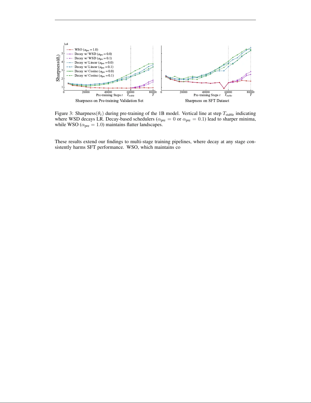
Published as a conference paper at ICLR 2026 P R E - T R A I N I N G L L M W I T H O U T L E A R N I N G R A T E D E C A Y E N H A N C E S S U P E R V I S E D F I N E - T U N I N G Kazuki Y ano † , Shun Kiyono ‡ , Sosuke K obayashi † , Sho T akase † , Jun Suzuki † † T ohoku Uni versity ‡ SB Intuitions yano.kazuki@dc.tohoku.ac.jp is-failab-research@grp.tohoku.ac.jp A B S T R AC T W e in vestig ate the role of learning rate scheduling in the large-scale pre-training of large language models, focusing on its influence on downstream performance af- ter supervised fine-tuning (SFT). Decay-based learning rate schedulers are widely used to minimize pre-training loss. Ho wev er , despite their widespread use, how these schedulers affect performance after SFT remains underexplored. In this pa- per , we examine W armup-Stable-Only (WSO), which maintains a constant learn- ing rate after warmup without an y decay . Through experiments with 1B and 8B parameter models, we show that WSO consistently outperforms decay-based schedulers in terms of performance after SFT , ev en though decay-based sched- ulers may exhibit better performance after pre-training. The result also holds across dif ferent regimes with mid-training and ov er-training. Loss landscape anal- ysis further re veals that decay-based schedulers lead models into sharper minima, whereas WSO preserves flatter minima that support adaptability . These findings indicate that applying LR decay to impro ve pre-training metrics may compromise downstream adaptability . Our work also provides practical guidance for training and model release strategies, highlighting that pre-training models with WSO en- hances their adaptability for downstream tasks. 1 I N T RO D U C T I O N Learning rate (LR) scheduling is arguably one of the most critical yet operationally challenging as- pects of large language model (LLM) pre-training. Although Cosine decay has been con ventionally employed in numerous models (Brown et al., 2020; Le et al., 2022; T ouvron et al., 2023a), it has prov en inflexible in recent training paradigms such as continual pre-training, as it requires heuristic tuning of the LR from the decayed v alue (H ¨ agele et al., 2024; Ibrahim et al., 2024). T o address this infle xibility , recent studies ha ve introduced W armup-Stable-Decay (WSD), which k eeps the LR constant through most of pre-training and decays it only briefly at the end (Hu et al., 2024; Liu et al., 2024a; W en et al., 2025). These previous studies, regardless of the details of the design choices, decayed the LRs to optimize the performance of pre-trained models. Ho we ver , the more critical factor for real applications is the performance after post-training, such as supervised fine-tuning (SFT). Drawing on the findings of Sun & Dredze (2025) and Springer et al. (2025), which sho w that a strong pre-training model does not necessarily imply superior performance after SFT , it is questionable to schedule LRs to the decayed value based on pre-training performance. In this study , we provide a comprehensive empirical in vestigation of LR schedulers during pre- training in terms of performance after SFT . In particular, we examine an underestimated schedul- ing, W armup-Stable-Only (WSO), which removes the decay phase from WSD and maintains con- stant LR to the end. W e sho w that WSO consistently achie ves superior performance after SFT compared to decay-based schedulers, through experiments on 1B and 8B models (Figure 1). Fur - thermore, we demonstrate that WSO is also effecti ve under modern training paradigms, including mid-training (OLMo et al., 2024; Meta, 2024c) and ov er-training (Sardana et al., 2024; Gadre et al., 2025). 1 Published as a conference paper at ICLR 2026   )(      )      )- - -  -(                              Figure 1: Learning rate schedulers used in pre-training and their impact on performance after su- pervised fine-tuning (SFT). W armup-Stable-Only (WSO), which remo ves the decay phase, achie ves the highest performance after SFT . T o understand why WSO yields superior SFT performance, we draw on insights from the transfer learning literature (Ju et al., 2022; Liu et al., 2023), which suggest that models in flatter regions of the loss landscape tend to exhibit better adaptability . Through an analysis of sharpness v alues, we sho w that models trained with WSO reside in flatter regions than those trained with other decay-based LR schedulers, and are therefore more adaptable to post-training tasks. Our contributions are as follows: (1) W e provide the systematic demonstration that WSO consis- tently outperforms decay-based schedulers on downstream tasks after SFT , with comprehensiv e evidence across 1B and 8B models and div erse ev aluation benchmarks. (2) W e show that WSO similarly benefits mid-training and ov er-training scenarios, achie ving superior SFT performance compared to con ventional decay-based schedulers. (3) W e re veal through loss landscape analysis that WSO preserves flatter minima than decay-based schedulers, explaining why models trained with WSO achiev e better performance after SFT . 2 P R E L I M I NA R I E S Recent LLMs are typically built with a staged training scheme. The most common and fundamental training pipeline consists of two stages, namely pre-training and post-training. In this section, we de- scribe these training stages and revie w the LR schedulers commonly employed during pre-training. Pre-training . Pre-training forms the foundation of LLM dev elopment, where models learn general language understanding from massiv e text corpora by minimizing the next-token prediction loss. Recently , pre-training has sometimes consisted of multiple stages: standard pre-training and mid- training (OLMo et al., 2024). W e describe mid-training in detail later (Section 2.2), and conduct experiments with both the standard pre-training and the multi-stage setup. Post-training . Post-training adapts pre-trained models to tar get tasks, enabling them to follow human instructions and av oid generating harmful outputs. Post-training includes techniques such as supervised fine-tuning (SFT), preference tuning (e.g., DPO (Rafailov et al., 2023)), and RL-based alignment (Ouyang et al., 2022). While post-training could be a multi-stage process with many design choices still under activ e exploration, SFT is relativ ely standardized and serves a core stage. In this paper , we focus on SFT as the canonical post-training stage and ev aluate the performance after SFT 1 . 2 . 1 T A S K D E FI N I T I O N Practically , LLM developers ev aluate models at multiple stages, selecting the best-performing one as the starting point for the subsequent stage. W e define Task s ( M ) as a function that, for a given LLM M , returns the performance on a set of pre-defined tasks used to assess the target stage s , where 1 The computational cost of pre-training is typically much larger than that of other stages, so identifying a better pre-training configuration has a substantial impact on the efficienc y of LLM construction. In this study , we focus on ev aluating LR schedulers during large-scale pre-training and characterize the potential of non-decay schedulers based on the performance after SFT . An exploration of complex combinations of LR scheduling spanning multiple post-training stages is left to future work. 2 Published as a conference paper at ICLR 2026 s ∈ { pre , post } denotes the training stage, with pre indicating pre-training and p ost indicating post- training, respectiv ely . W e write M 2 [ M 1 ] to denote the model M 2 trained with some configuration and initialization with M 1 , where M rand indicates a model whose weights are randomly initial- ized. Moreover , we introduce M pre and M post to represent the sets of models obtained through pre-training and post-training, respectiv ely , with various hyperparameter configurations. A typical training pipeline for building LLMs can therefore be e xpressed as follo ws: c M pre = arg max M pre ∈M pre { Task pre ( M pre [ M rand ]) } , c M post = arg max M post ∈M post n Task post ( M post [ c M pre [ M rand ]]) o . (1) This formulation may lead to a suboptimal solution in terms of the performance of the final model, namely , c M post , since selecting the best-performing models at intermediate stages does not guarantee achieving the best performance in the end. Therefore, conceptually , we would like to consider the following search problem to obtain a better final model for this training pipeline: c M post = arg max ( M pre ,M post ) ∈ ( M pre , M post ) { Task post ( M post [ M pre [ M rand ]]) } . (2) The primary objectiv e of this paper is to empirically examine the search problem by ev aluating sev eral LR schedulers during the lar ge-scale training stages that precede post-training. 2 . 2 F U RT H E R C O N S I D E R AT I O N S Mid-training. Mid-training has emerged as a critical intermediate stage in modern language model development, occupying a computational middle ground between large-scale pre-training and task-specific post-training (Meta, 2024c; OLMo et al., 2024). This stage serves multiple strategic objectiv es, including domain expansion and long-conte xt extension. For e xample, OLMo 2 (OLMo et al., 2024) demonstrates performance gains through mid-training on curated high-quality data, es- tablishing this stage as an essential component of the modern training pipeline. After introducing mid-training, we can rewrite equation 2 as follo ws: c M post = arg max ( M pre ,M mid ,M post ) ∈ ( M pre , M mid , M post ) { Task post ( M post [ M mid [ M pre [ M rand ]]]) } . (3) Over -training. Modern LLMs are often trained on trillions of tokens, far beyond the Chinchilla compute-optimal regime of roughly 20 tokens per parameter (Hoffmann et al., 2022). This practice trades substantially more training compute for improved inference efficienc y at deployment. Recent production systems use hundreds to thousands of tokens per parameter (Sardana et al., 2024). While full-scale experiments are costly , Section 5 presents results under such a configuration, showing the generality of our main findings. 2 . 3 C U R R E N T L R S C H E D U L I N G P R A C T I C E S In current LLM training practice, pre-training uses decay-based LR schedulers with Cosine, Lin- ear , or WSD that reduce LR to 0–10% of maximum (T ouvron et al., 2023a; Hu et al., 2024; Bergsma et al., 2025). Additionally , in mid-training, it is common practice to further decay the LR from the final v alue reached at the end of the preceding pre-training phase (Meta, 2024c; OLMo et al., 2024). These schedulers are chosen to minimize loss at each respectiv e stage, ef fectiv ely optimizing Task pre ( M pre ) independently . Howe ver , the primary objectiv e should be to maximize Task post ( M post ) , the performance after the complete pipeline. Thus, optimizing for Task pre ( M pre ) may be suboptimal. F or instance, recent findings from Springer et al. (2025) and Sun & Dredze (2025) rev eal that the better performance after pre-training does not guarantee performance after SFT . These raise a fundamental question: Is LR decay , which is chosen based on pr e-training per- formance, still the best choice when the model will under go supervised fine-tuning? Our work in- vestigates this question by systematically varying LR schedulers in M pre and M mid to understand their impact on the final objectiv e, i.e., Task post ( M post ) . 3 Published as a conference paper at ICLR 2026 2 . 4 F O R M A L I Z AT I O N O F L E A R N I N G R AT E S C H E D U L E R S W e denote the LR at training step t as η Scheduler ( t, α pre ) , where Scheduler specifies the LR scheduler and α pre controls the minimum LR factor in pre-training. For example, the WSD scheduler is defined as: η WSD ( t, α pre ) =      η max · t T warmup t ≤ T warmup η max T warmup < t ≤ T stable η max ·  (1 − α pre ) · T pre − t T pre − T stable + α pre  T stable < t ≤ T pre (4) where η max is the maximum LR, T pre denotes the total number of pre-training steps, T warmup is the number of warmup steps, and T stable is the step at which the decay phase begins. T o in vestigate the effecti veness of the LR scheduler without decay , we consider a simple variant of WSD, which we call W armup-Stable-Only (WSO). In this variant, the decay phase is omitted, which corresponds to setting α pre = 1 . 0 . η WSO ( t, α pre ) = ( η max · t T warmup t ≤ T warmup η max T warmup < t ≤ T pre (5) In our experiments, we in vestigate four LR schedulers: Scheduler ∈ { WSO , WSD , Cosine , Linear } . The detailed formulations for Cosine η Cosine ( t, α pre ) and Linear η Linear ( t, α pre ) are provided in Appendix B. T pre Training Steps t 0 η max Learning Rate 0.1 × η max η * α pre α mid WSO, 1.0, 1.0 WSD, 0.1, 0.0 Linear, 0.1, 0.0 Linear, 0.1, 1.0 Cosine, 0.1, 0.0 Cosine, 0.1, 1.0 Figure 2: Mid-training LR schedulers with different α pre and α mid values. LR Scheduling in Mid-training. W e parameterize mid-training schedulers with α mid (Figure 2), where α mid = 0 . 0 applies Linear decay to zero while α mid = 1 . 0 maintains the LR constant throughout mid-training. When combined with α pre = 1 . 0 , the configuration of α pre = 1 . 0 and α mid = 1 . 0 extends WSO across both pre-training and mid-training stages. The detailed formu- lation for mid-training LR schedulers is provided in Ap- pendix B. 3 E X P E R I M E N T 1 : T W O - S TAG E ( P R E - A N D P O S T - T R A I N I N G ) S E T T I N G W e in vestigate whether decaying LRs during pre-training truly benefit downstream SFT perfor - mance. 3 . 1 E X P E R I M E N TA L S E T U P Model Ar chitectures. W e conduct experiments on tw o model scales follo wing the Llama 3 archi- tecture family: 1B and 8B parameter models (same architecture as Llama-3.2-1B (Meta, 2024b) and Llama-3.1-8B (Meta, 2024a), respectiv ely). Full details are provided in Appendix A. Pre-training Configuration. Models are pre-trained on FineW eb-Edu (Penedo et al., 2024) with a maximum LR η max = 3 × 10 − 4 . W e in vestig ate three LR schedulers as formalized in Section 2.4, experimenting with WSO (Equation 2.4), WSD (Equation 2.4), Cosine, and Linear schedulers (de- tailed in Appendix B). For each scheduler , we vary the minimum LR factor α pre ∈ { 0 . 0 , 0 . 1 , 1 . 0 } , following our notation η Scheduler ( t, α pre ) . Setting α pre = 0 . 0 corresponds to decay to zero. Recent work by Bergsma et al. (2025) shows that this achie ves better pre-training performance. Setting α pre = 0 . 1 corresponds to decay to 10% of maximum, a choice commonly used in practice by Chin- chilla (Hoffmann et al., 2022), Llama 3 (Meta, 2024c) and OLMo 2 (OLMo et al., 2024). Finally , setting α pre = 1 . 0 corresponds to WSO. Further hyperparameter details are provided in Appendix C. 4 Published as a conference paper at ICLR 2026 T able 1: Relativ e performance across pre-training (PT) and supervised fine-tuning (SFT). For each model size and each metric, v alues are dif ferences ( ∆ ) from the best-performing decay-based sched- uler for that metric. Note that WSO could perform poorly after PT but best after SFT . Bold indicates the best performance. Model Scheduler α pre PT V alid Loss ↓ ∆ PT T ask A vg ∆ SFT T ask A vg ∆ 1B W armup-Stable-Only (WSO) 1.0 +0.071 -1.7 +0.3 WSD 0.1 +0.004 -1.5 +0.0 0.0 +0.000 -1.2 -1.0 Linear 0.1 +0.021 -2.0 -0.7 0.0 +0.016 +0.0 -0.9 Cosine 0.1 +0.019 -0.1 -0.7 0.0 +0.016 -2.5 -0.7 8B W armup-Stable-Only (WSO) 1.0 +0.127 -0.8 +1.1 WSD 0.1 +0.019 -0.2 -0.8 0.0 +0.014 +0.0 -0.3 Linear 0.1 +0.013 -1.9 -0.6 0.0 +0.000 -1.8 +0.0 Cosine 0.1 +0.009 -2.2 -0.3 0.0 +0.008 -2.3 -0.1 SFT Configuration. W e perform SFT using the T ulu-3 SFT mixture 2 . W e conduct a comprehen- siv e LR sweep ranging from 5 × 10 − 7 to 1 × 10 − 3 to identify the best hyperparameters for each pre-trained model 3 . Evaluation. W e ev aluate models at two stages: after pre-training and after SFT . F or pre-trained models, we assess zero-shot performance on standard benchmarks, including question answer- ing (ARC-Easy , ARC-Challenge (Clark et al., 2018), OpenBookQA (Mihaylov et al., 2018), BoolQ (Clark et al., 2019)) and commonsense reasoning (HellaSw ag (Zellers et al., 2019), PIQA (Bisk et al., 2020), W inoGrande (Sakaguchi et al., 2021)), along with v alidation loss. For fine-tuned models, we follow the setup of OLMo (Groenev eld et al., 2024) and ev aluate along three key dimensions: instruction-follo wing capability (AlpacaEval (Li et al., 2023)), multi-task language understanding (MMLU (Hendrycks et al., 2021)), and truthfulness (T ruthfulQA (Lin et al., 2022)). T o highlight ho w LR decay affects both pre-training and SFT dif ferently , we present results as relativ e performance metrics normalized against the best decay-based scheduler for each stage. For pre-training, we report both v alidation loss and the average accuracy across all zero-shot benchmarks (PT T ask A vg). For fine-tuning, we report the a verage across AlpacaEv al, T ruthfulQA, and MMLU (SFT T ask A vg) 4 . 3 . 2 R E S U L T S T able 1 shows an inv ersion in model performance across training stages 5 . For pre-training perfor- mance, decay-based schedulers achiev e the best performance with α pre = 0 . Specifically , Linear and WSD with α pre = 0 achie ve the best PT T ask A vg scores for the 1B and 8B models, respec- tiv ely . This result is consistent with existing findings (Bergsma et al., 2025). In contrast, after SFT , WSO achiev es the best performance for both model sizes, even though it underperforms decay-based schedulers in pre-training metrics. These results demonstrate that while decay-bas ed schedulers may 2 https://huggingface.co/datasets/allenai/tulu- 3- sft- olmo- 2- mixture/ tree/main 3 Full details about SFT are provided in Appendix D. 4 Detailed ev aluation settings are provided in Appendix E. 5 Detailed per-task e v aluation results for all models are provided in Appendix F. 5 Published as a conference paper at ICLR 2026 T able 2: Relati ve performance across mid-training (MT) and SFT stages. V alues are dif ferences from the best decay-based schedule. WSO throughout both stages yields the best SFT performance. Model (Pre-training) Scheduler α pre α mid MT V alid Loss ↓ ∆ MT T ask A vg ∆ SFT T ask A vg ∆ 1B W armup-Stable-Only (WSO) 1.0 1.0 +0.062 -0.1 +0.8 WSD 1.0 0.0 +0.000 + 0.0 +0.0 0.1 1.0 +0.038 -1.5 -0.5 0.1 0.0 +0.047 -1.7 -1.3 Linear 0.1 1.0 +0.053 -2.1 -2.5 0.1 0.0 +0.058 -3.3 -3.8 Cosine 0.1 1.0 +0.053 -2.4 -2.9 0.1 0.0 +0.059 -3.1 -3.7 8B W armup-Stable-Only (WSO) 1.0 1.0 +0.102 -2.1 +1.1 WSD 1.0 0.0 +0.000 +0.0 -1.4 0.1 1.0 +0.057 -5.0 +0.0 0.1 0.0 +0.081 -5.6 -1.1 Linear 0.1 1.0 +0.067 -8.3 -2.2 0.1 0.0 +0.082 -9.0 -3.7 Cosine 0.1 1.0 +0.068 -8.0 -3.5 0.1 0.0 +0.084 -10.1 -4.1 yield superior performance in terms of pre-training metrics, WSO is more effecti v e in the overall training pipeline, including SFT . 4 E X P E R I M E N T 2 : T H R E E - S TAG E ( P R E - , M I D - , A N D P O S T - T R A I N I N G ) S E T T I N G Recent LLM dev elopments (OLMo et al., 2024; Meta, 2024c) add a mid-training stage between pre-training and post-training, which makes LR scheduling across stages more complex due to the various combinations of pre-training and mid-training LR schedulers. W e in v estigate whether using WSO in both pre-training and mid-training stages yields better performance after SFT than decay- based schedulers. 4 . 1 E X P E R I M E N TA L S E T U P T o in vestigate the effect of LR scheduling during mid-training, we conduct e xperiments follo wing a three-stage training pipeline: pre-training, mid-training, and post-training. W e systematically vary the LR schedulers in both pre-training and mid-training stages to understand their individual and combined effects on downstream performance. T o ensure comparability with recent mid-training work, our setup largely follows OLMo 2 (OLMo et al., 2024), a representativ e study of mid-training. Pre-training Stage. W e pre-train 1B and 8B models using the same architecture and configuration as described in Section 3. W e adopt pre-training dataset olmo-mix-1124 (OLMo et al., 2024) used in OLMo 2. Follo wing standard practice in modern LLM de velopment (Meta, 2024c; OLMo et al., 2024), we employ four LR schedulers with dif ferent minimum LR factors, including WSD, Cosine, and Linear schedulers with α pre = 0 . 1 , and additionally WSO. Mid-training Stage and Learning Rate Schedules. F ollo wing OLMo 2 (OLMo et al., 2024), we conduct mid-training on the dolmino-mix-1124 dataset. W e inv estigate the two mid-training strategies shown in Figure 2, with α mid = 0 . 0 applying further Linear decay following common practice (Meta, 2024c; OLMo et al., 2024), and α mid = 1 . 0 maintaining a constant LR throughout mid-training 6 . 6 Further training configurations of mid-training are provided in Appendix G. 6 Published as a conference paper at ICLR 2026 T able 3: Relativ e performance after over -training (2T tokens). V alues are differences ( ∆ ) from the best-performing decay-based scheduler for each metric. Similar to Section 3, WSO achieves the best SFT performance. Model Scheduler α pre PT V alid Loss ↓ ∆ PT T ask A vg ∆ SFT T ask A vg ∆ 1B W armup-Stable-Only (WSO) 1.0 + 0.048 - 1.5 +0.7 WSD 0.1 +0.004 +0.0 +0.0 0.0 +0.000 +0.0 -0.3 Linear 0.1 +0.021 -0.9 -0.5 0.0 +0.017 -0.4 -0.6 Cosine 0.1 +0.017 +0.0 -0.4 0.0 +0.017 -1.3 -0.3 T able 4: Relativ e performance after ov er-training with mid-training (2T + 500B tokens). V alues are differences ( ∆ ) from the best-performing decay-based scheduler for each metric. Similar to Section 4, WSO yields the best SFT performance. Model (Pre-training) Scheduler α pre α mid MT V alid Loss ↓ ∆ MT T ask A vg ∆ SFT T ask A vg ∆ 1B W armup-Stable-Only (WSO) 1.0 1.0 +0.055 -0.3 +1.4 WSD 1.0 0.0 +0.000 -1.6 -0.5 0.1 1.0 +0.033 + 0.0 -1.0 0.1 0.0 +0.038 -1.7 -1.2 Linear 0.1 1.0 +0.068 -2.2 +0.0 0.1 0.0 +0.051 -2.8 -0.6 Cosine 0.1 1.0 +0.046 -1.8 -0.7 0.1 0.0 +0.054 -2.3 -1.2 SFT and Evaluation. For SFT , we follow the configuration described in Section 3. For mid- trained models (before SFT), we ev aluate on standard benchmarks to assess the impact of mid- training LR schedulers, follo wing the e valuation suite used in OLMo 2 (OLMo et al., 2024). W e select benchmarks that comprehensiv ely assess model capabilities, including reasoning tasks (ARC-Challenge (Clark et al., 2018), HellaSwag (Zellers et al., 2019), WinoGrande (Sakaguchi et al., 2021)), reading comprehension (DR OP (Dua et al., 2019)), and mathematical reasoning (GSM8K (Cobbe et al., 2021)). Follo wing SFT , we assess models using an expanded ev aluation suite including AlpacaEval (Li et al., 2023) for instruction following, T ruthfulQA (Lin et al., 2022) for factual accuracy , GSM8K (Cobbe et al., 2021) for mathematical reasoning, DROP (Dua et al., 2019) for reading comprehension, AGI Eval (Zhong et al., 2024) for general intelligence capabili- ties, BigBench-Hard (Suzgun et al., 2023) for challenging reasoning tasks, and MMLU for multitask understanding 7 . Similar to Section 3, we present results as relative improvements compared to the best decay-based scheduler . 4 . 2 R E S U L T S T able 2 sho ws an inv ersion similar to our pre-training findings 8 . For mid-training performance, the decay-based scheduler with α pre = 1 . 0 and α mid = 0 . 0 achiev e the best performance. Howe ver , SFT performance again shows the opposite trend. WSO achiev es the best downstream task performance after SFT , e ven though it underperforms the best decay-based schedulers in mid-training metrics. Additionally , we find that introducing decay at any stage reduces SFT performance. Notably , for models pre-trained with decay ( α pre = 0 . 1 ), a voiding decay during mid-training ( α mid = 1 . 0 ) im- prov es both mid-training metrics and SFT performance compared to applying decay . 7 The detailed ev aluation settings for these benchmarks are described in Appendix E. 8 Detailed per-task e v aluation results for all models are provided in Appendix F. 7 Published as a conference paper at ICLR 2026 0 20000 40000 60000 80000 P r e - t r a i n i n g S t e p s t 1 2 3 4 5 S h a r p n e s s ( t ) 1e4 T s t a b l e T Sharpness on Pre-training V alidation Set W S O ( p r e = 1 . 0 ) D e c a y w / W S D ( p r e = 0 . 0 ) D e c a y w / W S D ( p r e = 0 . 1 ) D e c a y w / L i n e a r ( p r e = 0 . 0 ) D e c a y w / L i n e a r ( p r e = 0 . 1 ) D e c a y w / C o s i n e ( p r e = 0 . 0 ) D e c a y w / C o s i n e ( p r e = 0 . 1 ) 0 20000 40000 60000 80000 P r e - t r a i n i n g S t e p s t T s t a b l e T Sharpness on SFT Dataset Figure 3: Sharpness ( θ t ) during pre-training of the 1B model. V ertical line at step T stable indicating where WSD decays LR. Decay-based schedulers ( α pre = 0 or α pre = 0 . 1 ) lead to sharper minima, while WSO ( α pre = 1 . 0 ) maintains flatter landscapes. These results extend our findings to multi-stage training pipelines, where decay at any stage con- sistently harms SFT performance. WSO, which maintains constant learning rates throughout both pre-training and mid-training, sho ws the best performance across the overall training pipeline, in- cluding mid-training and SFT . 5 E X P E R I M E N T 3 : T H R E E - S TAG E S E T T I N G I N T H E O V E R - T R A I N I N G T o further probe generality , we ev aluate a third regime with a substantially larger training budget. This over -training setting serves as a test of whether the benefits of WSO persist when training on trillions of tokens. 5 . 1 E X P E R I M E N TA L S E T U P Pre- and Mid-training. W e pre-train 1B models on 2T tokens, which is approximately 100 × the Chinchilla-optimal amount of data for this model size, to ev aluate whether WSO maintains its advantages at this data scale. W e use the same datasets as in Sections 3 and 4 for pre-training and mid-training, respectively . W e in vestigate the same set of LR schedulers as in Section 3. W e additionally conduct mid-training experiments using 500B tokens, following the same e xperimental setup as in Section 4. Evaluation. W e ev aluate all LR schedulers using the same methodology as in Sections 3 and 4, measuring performance both after pre-training (or mid-training) and after SFT . Detailed configura- tions are provided in Appendices C and D. 5 . 2 R E S U L T S T ables 3 and 4 confirm that the in version observed in Sections 3 and 4 persists e ven in the ov er- training regime using 2T tokens. Across all inv estigated schedulers, WSO ( α pre = 1 . 0 ) consis- tently yields worse intermediate metrics but superior SFT performance compared to decay-based schedulers. Similar to our earlier findings, decay-based schedulers achiev e better pre-training and mid-training metrics, yet WSO outperforms them after SFT . This pattern holds both for single-stage ov er-training (T able 3) and when combined with mid-training (T able 4), demonstrating that the ben- efits of WSO are robust across dif ferent data scales and training configurations. 6 U N D E R S T A N D I N G A DA P TA B I L I T Y T H RO U G H L O S S L A N D S C A P E G E O M E T RY T o understand why models trained with WSO achiev e superior SFT performance, we analyze the loss landscape geometry throughout the pre-training phase. As suggested in the transfer learning 8 Published as a conference paper at ICLR 2026 literature (Ju et al., 2022; Liu et al., 2023), we focus on sharpness as a key geometric property that characterizes the curvature of the loss landscape around con ver ged parameters. The relation between lo wer sharpness and better SFT performance stems from ho w models respond to parameter updates during fine-tuning. When the parameters of the model lie in a flatter region of the loss landscape, which corresponds to lower sharpness, the model demonstrates superior adapt- ability to downstream tasks (Foret et al., 2021; Li et al., 2025). The intuition is that the performance of the model remains stable during the parameter updates of SFT . A model in a flat landscape e xpe- riences less fluctuation in its loss value when its parameters are updated, which translates to more stable performance. This characteristic is belie ved to confer higher adaptability , as the model can in- corporate ne w data without compromising its pre-trained capabilities (Andriushchenk o et al., 2023). There are several ways to quantify sharpness, such as the largest eigenv alue of the Hessian (captur- ing the most curved direction) or the trace of the Hessian (capturing the average curvature) (Dinh et al., 2017; Kaur et al., 2023). Following established practice in optimization and generalization studies (Ju et al., 2022; Liu et al., 2023), we adopt the trace as our sharpness measure, since it provides a scalar summary of curv ature across all parameter dimensions. Definition 6.1 (Sharpness) . Let L ( θ t ; D ) denote the loss function ev aluated on dataset D with model parameters θ t ∈ R d . At training step t , the sharpness of the loss landscape at parameters θ t is defined as the trace of the Hessian matrix: Sharpness ( θ t ) = T r( H L ( θ t )) = d X i =1 ∂ 2 L ( θ t ; D ) ∂ θ 2 i (6) where H L ( θ t ) ∈ R d × d is the Hessian matrix of the loss with respect to the parameters at θ t . Since computing the full Hessian trace is computationally prohibitiv e for billion-parameter models, we employ Hutchinson’ s unbiased estimator (Hutchinson, 1989; Liu et al., 2024b). This method requires only Hessian-vector products, which can be ef ficiently computed through automatic differ - entiation. Details of our sampling procedure and computational details are provided in Appendix H. W e measure sharpness throughout pre-training on validation sets from both the pre-training dataset and the SFT dataset. Figure 3 shows the sharpness for the 1B model from Section 3. W e illustrate a vertical line at step T stable to indicate the point at which WSD decays LR. The figure re veals distinct patterns across schedulers. Specifically , Cosine and Linear schedulers exhibit steadily increasing sharpness as the LR decays, while WSD shows a rise during its decay phase. In contrast, WSO maintains lower sharpness. Across both datasets, models with decaying LRs conv erge to regions with about 2–3 × higher sharpness compared to WSO models. Flatter regions obtained by WSO allow more fle xible parameter adaptation during SFT , enabling better downstream performance. 0 10000 20000 30000 40000 50000 S h a r p n e s s ( T ) 52.5 53.0 53.5 54.0 54.5 55.0 A vg. SFT Score P e a r s o n r = 0 . 7 0 9 W S O ( p r e = 1 . 0 ) W S D ( p r e = 0 . 1 ) W S D ( p r e = 0 . 0 ) L i n e a r ( p r e = 0 . 1 ) L i n e a r ( p r e = 0 . 0 ) C o s i n e ( p r e = 0 . 1 ) C o s i n e ( p r e = 0 . 0 ) Figure 4: Pre-training sharpness negati vely corre- lates with downstream SFT performance. Correlation between shar pness and down- stream adaptability . T o provide empirical evidence linking the loss landscape to down- stream adaptability , we analyze the correlation between the sharpness of pre-trained models and their subsequent SFT performance. Fig- ure 4 presents the SFT performance plotted against the sharpness measured on the pre- training validation set for the 1B model across all inv estigated learning rate schedulers. The analysis rev eals a negati ve correlation (Pearson r = − 0 . 709 ) between the sharpness of the min- ima and the model’ s performance after SFT . The WSO scheduler ( α pre = 1 . 0 ) resides in the low-sharpness, high-performance re gion, while decay-based schedulers conv erge to sharper minima with lower SFT scores. While the sample size is limited, this pattern is consistent with our hypothesis that preserving flatter minima during pre- training enhances the model’ s adaptability . 9 Published as a conference paper at ICLR 2026 7 R E L A T E D W O R K Learning Rate Scheduling in LLM T raining. LR decay has been considered effecti ve for LLM pre-training, with Cosine decay remaining the de facto standard (Kaplan et al., 2020; Hoffmann et al., 2022; T ouvron et al., 2023b). Recent large-scale studies advocate for e ven more aggressive decay , showing that Linear decay to zero achie ves lower pre-training loss in compute-optimal set- tings (Bergsma et al., 2025). W armup-Stable-Decay (WSD) delays decay until the final phase of training (Hu et al., 2024), while theoretical analysis suggests that decay may confine models to narrow loss v alleys (W en et al., 2025). Some methods attempt to av oid the decay phase through checkpoint a veraging (San yal et al., 2024) or model mer ging (T ian et al., 2025). Jin et al. (2023) in- vestigated learning rate tuning strategies within individual training phases, b ut did not examine ho w pre-training LR choices propagate through to post-training performance. While these studies hav e advanced our understanding of LR scheduling within a single training phase, they share a common limitation: ev aluation is restricted to the phase in which the schedule is applied, without considering the downstream consequences for subsequent training stages such as SFT . Relationship to Continual Pr e-training and Fine-tuning Studies. Recent work on continual pre-training (CPT) has explored LR scheduling for domain adaptation. W ang et al. (2025) showed that models with higher loss potential achieve lower CPT v alidation loss and adv ocated for re- leasing high loss potential versions to facilitate downstream tasks. W ang et al. (2024) proposed a path-switching paradigm for LR scheduling in model version updates, though their experimental setup still applies LR decay before performing SFT . T issue et al. (2024) introduced a scaling law describing loss dynamics in relation to learning rate annealing; howe v er , they explicitly note that post-training scenarios in v olving distribution shift are out of scope. These CPT studies focus on settings where the objectiv e function remains language modeling, leaving the impact on SFT unex- plored. Meanwhile, a gro wing body of work has examined the gap between pre-training quality and downstream performance more broadly . Sun & Dredze (2025) showed that stronger pre-training per- formance does not necessarily translate to superior fine-tuning outcomes, and Springer et al. (2025) demonstrated that over -trained models become harder to fine-tune. These findings collectively mo- tiv ate our in vestig ation, as LR schedulers chosen to optimize potentially unreliable pre-training met- rics may not be optimal for the overall training pipeline. Our work identifies LR decay as a specific factor that improv es pre-training metrics at the cost of do wnstream adaptability . Adaptability and Loss Landscape Geometry . Early work showed that parameters in flatter loss regions generalize better than those in sharp minima (Keskar et al., 2017), motiv ating sharpness- aware minimization (Foret et al., 2021) and stochastic weight averaging (Izmailov et al., 2018). Recent theoretical advances explain WSD through a riv er valley loss landscape perspectiv e (W en et al., 2025), where the stable phase e xplores along the v alley floor while the decay phase con verges tow ard the center . Concurrent work confirmed that sharpness increase during decay is univ ersal across architectures (Belloni et al., 2025). Flat-minima optimizers work well under distrib ution shift (Kaddour et al., 2022), a property that extends to the pre-training/fine-tuning paradigm, where the fine-tuning data distribution dif fers substantially from pre-training (Ju et al., 2022; Liu et al., 2023). While prior work focused on understanding sharpness dynamics during pre-training (Bel- loni et al., 2025; W en et al., 2025), we demonstrate how these dynamics concretely impact SFT performance, showing that WSO preserv es flatness and enhances do wnstream adaptability . 8 C O N C L U S I O N In this study , we in vestig ated the effecti veness of LR schedulers, which have been widely reported as ef fectiv e for pre-training, in practical scenarios with a focus on post-training performance. In particular , we examine W armup-Stable-Only (WSO), which remov es the decay phase from WSD. Experimental results show that WSO consistently outperforms decay-based schedulers in down- stream tasks after SFT across standard pre-training, mid-training, and over -training regimes. Loss landscape analysis further rev eals that WSO preserves flatter minima, explaining its superior adapt- ability . WSO is simple to apply and yields impro ved post-training performance, making it a promis- ing alternativ e for constructing more portable models. W e also recommend releasing LLMs trained with WSO so that practitioners can benefit from their adaptability . 10 Published as a conference paper at ICLR 2026 E T H I C S S TA T E M E N T This work inv estigates learning rate scheduling for LLM training to impro ve downstream adaptabil- ity . While our methods may provide new findings on LR scheduling on pre-training, we acknowl- edge the broader implications of adv ancing LLM capabilities. W e encourage responsible deploy- ment with appropriate safety measures during post-training. W e exclusi vely used publicly av ailable datasets for pre-training, supervised fine-tuning, and evaluation. Moreov er , we de veloped the lan- guage models entirely from scratch, av oiding the use of any publicly av ailable models to ensure reproducibility . R E P RO D U C I B I L I T Y S TA T E M E N T T o ensure reproducibility of our results, we provide comprehensi ve experimental details throughout the paper and appendices. Model architectures for both 1B and 8B parameter models are specified in Appendix A, including all layer configurations and attention mechanisms. All pre-training hyper- parameters, including optimizer settings, batch sizes, and training steps, are detailed in Appendix C. The supervised fine-tuning configuration, including the learning rate sweep range and ev aluation protocols, is described in Appendix D. Our sharpness computation methodology using Hutchin- son’ s estimator is fully specified in Appendix H. W e use publicly available datasets (FineW eb-Edu, olmo-mix-1124, dolmino-mix-1124, and T ulu-3 SFT mixture) and standard e v aluation benchmarks, with detailed ev aluation settings provided in Appendix E. Full numerical results for all experiments are reported in Appendix F to facilitate comparison and v alidation. A C K N O W L E D G M E N T S This work was partly supported by JST Moonshot R&D Grant Number JPMJMS2011-35 (funda- mental research). R E F E R E N C E S Maksym Andriushchenko, Francesco Croce, Maximilian M ¨ uller , Matthias Hein, and Nicolas Flam- marion. A modern look at the relationship between sharpness and generalization. In Andreas Krause, Emma Brunskill, Kyunghyun Cho, Barbara Engelhardt, Si van Sabato, and Jonathan Scar - lett (eds.), Pr oceedings of the 40th International Conference on Machine Learning , volume 202 of Proceedings of Machine Learning Resear c h , pp. 840–902. PMLR, 23–29 Jul 2023. URL https://proceedings.mlr.press/v202/andriushchenko23a.html . Annalisa Belloni, Lorenzo Noci, and Antonio Orvieto. Univ ersal dynamics of w armup stable decay: understanding WSD beyond transformers. In ICML 2025 W orkshop on Methods and Opportuni- ties at Small Scale , 2025. URL https://openreview.net/forum?id=2HNQqMBvC2 . Shane Bergsma, Nolan Simran Dey , Gurpreet Gosal, Gavia Gray , Daria Sobolev a, and Joel Hes- tness. Straight to zero: Why linearly decaying the learning rate to zero works best for LLMs. In The Thirteenth International Conference on Learning Representations , 2025. URL https: //openreview.net/forum?id=hrOlBgHsMI . Y onatan Bisk, Row an Zellers, Ronan bras, Jianfeng Gao, and Choi Y ejin. Piqa: Reasoning about physical commonsense in natural language. Pr oceedings of the AAAI Confer ence on Artificial Intelligence , 34:7432–7439, 04 2020. doi: 10.1609/aaai.v34i05.6239. T om Bro wn, Benjamin Mann, Nick Ryder, Melanie Subbiah, Jared D Kaplan, Prafulla Dhari- wal, Arvind Neelakantan, Prana v Shyam, Girish Sastry , Amanda Askell, Sandhini Agar- wal, Ariel Herbert-V oss, Gretchen Krue ger , T om Henighan, Rewon Child, Aditya Ramesh, Daniel Ziegler , Jeffre y W u, Clemens W inter , Chris Hesse, Mark Chen, Eric Sigler , Mateusz Litwin, Scott Gray , Benjamin Chess, Jack Clark, Christopher Berner, Sam McCandlish, Alec Radford, Ilya Sutsk ev er , and Dario Amodei. Language models are few-shot learners. In H. Larochelle, M. Ranzato, R. Hadsell, M.F . Balcan, and H. Lin (eds.), Advances in Neu- ral Information Processing Systems , volume 33, pp. 1877–1901. Curran Associates, Inc., 2020. URL https://proceedings.neurips.cc/paper_files/paper/2020/ file/1457c0d6bfcb4967418bfb8ac142f64a- Paper.pdf . 11 Published as a conference paper at ICLR 2026 Christopher Clark, Kenton Lee, Ming-W ei Chang, T om Kwiatk owski, Michael Collins, and Kristina T outanova. BoolQ: Exploring the surprising dif ficulty of natural yes/no questions. In Jill Burstein, Christy Doran, and Thamar Solorio (eds.), Pr oceedings of the 2019 Confer ence of the North American Chapter of the Association for Computational Linguistics: Human Lan- guage T echnologies, V olume 1 (Long and Short P apers) , pp. 2924–2936, Minneapolis, Min- nesota, June 2019. Association for Computational Linguistics. doi: 10.18653/v1/N19- 1300. URL https://aclanthology.org/N19- 1300/ . Peter Clark, Isaac Cowhe y , Oren Etzioni, T ushar Khot, Ashish Sabharwal, Carissa Schoenick, and Oyvind T afjord. Think you ha ve solv ed question answering? try arc, the ai2 reasoning challenge, 2018. Karl Cobbe, V ineet K osaraju, Mohammad Bav arian, Mark Chen, Heewoo Jun, Lukasz Kaiser , Matthias Plappert, Jerry T worek, Jacob Hilton, Reiichiro Nakano, et al. Training verifiers to solve math word problems. arXiv preprint , 2021. Laurent Dinh, Razvan Pascanu, Samy Bengio, and Y oshua Bengio. Sharp minima can generalize for deep nets. In International Conference on Mac hine Learning , pp. 1019–1028. PMLR, 2017. Dheeru Dua, Y izhong W ang, Pradeep Dasigi, Gabriel Stanovsky , Sameer Singh, and Matt Gardner . DR OP: A reading comprehension benchmark requiring discrete reasoning o ver paragraphs. In Jill Burstein, Christy Doran, and Thamar Solorio (eds.), Pr oceedings of the 2019 Conference of the North American Chapter of the Association for Computational Linguistics: Human Languag e T echnologies, V olume 1 (Long and Short P apers) , pp. 2368–2378, Minneapolis, Minnesota, June 2019. Association for Computational Linguistics. doi: 10.18653/v1/N19- 1246. URL https: //aclanthology.org/N19- 1246/ . Pierre Foret, Ariel Kleiner , Hossein Mobahi, and Behnam Neyshab ur . Sharpness-a ware minimiza- tion for ef ficiently improving generalization. In International Confer ence on Learning Repr esen- tations , 2021. URL https://openreview.net/forum?id=6Tm1mposlrM . Samir Y itzhak Gadre, Georgios Smyrnis, V aishaal Shankar , Suchin Gururangan, Mitchell W orts- man, Rulin Shao, Jean Mercat, Alex Fang, Jeffre y Li, Sedrick Keh, Rui Xin, Marianna Nezhu- rina, Igor V asilje vic, Luca Soldaini, Jenia Jitsev , Alex Dimakis, Gabriel Ilharco, Pang W ei K oh, Shuran Song, Thomas Kollar , Y air Carmon, Achal Dav e, Reinhard Heckel, Niklas Muennighoff, and Ludwig Schmidt. Language models scale reliably with over-training and on downstream tasks. In The Thirteenth International Conference on Learning Repr esentations , 2025. URL https://openreview.net/forum?id=iZeQBqJamf . Dirk Groeneveld, Iz Beltagy , Evan W alsh, Akshita Bhagia, Rodne y Kinney , Oyvind T afjord, Anan ya Jha, Hamish Ivison, Ian Magnusson, Y izhong W ang, Shane Arora, David Atkinson, Russell Au- thur , Khyathi Chandu, Arman Cohan, Jennifer Dumas, Y anai Elazar , Y uling Gu, Jack Hessel, T ushar Khot, W illiam Merrill, Jacob Morrison, Niklas Muennighoff, Aakanksha Naik, Crys- tal Nam, Matthe w Peters, V alentina Pyatkin, Abhilasha Ravichander , Dustin Schwenk, Saurabh Shah, W illiam Smith, Emma Strubell, Nishant Subramani, Mitchell W ortsman, Pradeep Dasigi, Nathan Lambert, K yle Richardson, Luke Zettlemoyer , Jesse Dodge, Kyle Lo, Luca Soldaini, Noah Smith, and Hannaneh Hajishirzi. OLMo: Accelerating the science of language models. In Lun-W ei Ku, Andre Martins, and V ivek Srikumar (eds.), Pr oceedings of the 62nd Annual Meet- ing of the Association for Computational Linguistics (V olume 1: Long P apers) , pp. 15789–15809, Bangkok, Thailand, August 2024. Association for Computational Linguistics. doi: 10.18653/v1/ 2024.acl- long.841. URL https://aclanthology.org/2024.acl- long.841/ . Alex H ¨ agele, Elie Bakouch, Atli K osson, Leandro V on W erra, Martin Jaggi, et al. Scaling laws and compute-optimal training beyond fixed training durations. Advances in Neural Information Pr ocessing Systems , 37:76232–76264, 2024. Dan Hendrycks, Collin Burns, Steven Basart, Andy Zou, Mantas Mazeika, Dawn Song, and Ja- cob Steinhardt. Measuring massive multitask language understanding. In International Confer- ence on Learning Repr esentations , 2021. URL https://openreview.net/forum?id= d7KBjmI3GmQ . 12 Published as a conference paper at ICLR 2026 Jordan Hof fmann, Sebastian Bor geaud, Arthur Mensch, Elena Buchatskaya, T revor Cai, Eliza Rutherford, Diego de las Casas, Lisa Anne Hendricks, Johannes W elbl, Aidan Clark, T om Hen- nigan, Eric Noland, Katherine Millican, George van den Driessche, Bogdan Damoc, Aurelia Guy , Simon Osindero, Karen Simonyan, Erich Elsen, Oriol V inyals, Jack W illiam Rae, and Laurent Sifre. An empirical analysis of compute-optimal large language model training. In Alice H. Oh, Alekh Agarwal, Danielle Belgrav e, and K yunghyun Cho (eds.), Advances in Neu- ral Information Pr ocessing Systems , 2022. URL https://openreview.net/forum?id= iBBcRUlOAPR . Shengding Hu, Y uge Tu, Xu Han, Chaoqun He, Ganqu Cui, Xiang Long, Zhi Zheng, Y ewei Fang, Y uxiang Huang, W eilin Zhao, et al. Minicpm: Un veiling the potential of small language models with scalable training strategies. arXiv pr eprint arXiv:2404.06395 , 2024. M.F . Hutchinson. A stochastic estimator of the trace of the influence matrix for laplacian smoothing splines. Communications in Statistics - Simulation and Computation , 18(3):1059– 1076, 1989. doi: 10.1080/03610918908812806. URL https://doi.org/10.1080/ 03610918908812806 . Adam Ibrahim, Benjamin Th ´ erien, Kshitij Gupta, Mats Leon Richter , Quentin Gregory Anthony , Eugene Belilovsk y , T imoth ´ ee Lesort, and Irina Rish. Simple and scalable strate gies to continually pre-train large language models. T ransactions on Mac hine Learning Resear ch , 2024. ISSN 2835- 8856. URL https://openreview.net/forum?id=DimPeeCxKO . Pa vel Izmailov , Dmitrii Podoprikhin, Timur Garipov , Dmitry V etrov , and Andrew Gordon Wilson. A veraging weights leads to wider optima and better generalization. In Confer ence on Uncertainty in Artificial Intelligence , pp. 876–885, 2018. Hongpeng Jin, W enqi W ei, Xuyu W ang, W enbin Zhang, and Y anzhao W u. Rethinking learning rate tuning in the era of large language models. In 2023 IEEE 5th International Conference on Cognitive Machine Intellig ence (CogMI) , pp. 112–121. IEEE, 2023. Haotian Ju, Dongyue Li, and Hongyang R Zhang. Robust fine-tuning of deep neural networks with hessian-based generalization guarantees. In Kamalika Chaudhuri, Stefanie Jegelka, Le Song, Csaba Szepesv ari, Gang Niu, and Siv an Sabato (eds.), Pr oceedings of the 39th International Confer ence on Machine Learning , volume 162 of Pr oceedings of Machine Learning Researc h , pp. 10431–10461. PMLR, 17–23 Jul 2022. URL https://proceedings.mlr.press/ v162/ju22a.html . Jean Kaddour , Linara Adilo v a K ey , Bernhard Sch ¨ olkopf, and Andrew Gordon W ilson. When do flat minima optimizers work? In Advances in Neural Information Processing Systems , volume 35, pp. 16577–16595, 2022. Jared Kaplan, Sam McCandlish, T om Henighan, T om B Brown, Benjamin Chess, Re won Child, Scott Gray , Alec Radford, Jeffre y W u, and Dario Amodei. Scaling laws for neural language models. arXiv preprint , 2020. Simran Kaur , Jeremy Cohen, and Zachary Chase Lipton. On the maximum hessian eigen v alue and generalization. In Javier Antor ´ an, Arno Blaas, Fan Feng, Sahra Ghalebikesabi, Ian Ma- son, Melanie F . Pradier, David Rohde, Francisco J. R. Ruiz, and Aaron Schein (eds.), Proceed- ings on ”I Can’t Believe It’ s Not Better! - Understanding Deep Learning Thr ough Empirical F alsification” at NeurIPS 2022 W orkshops , volume 187 of Pr oceedings of Machine Learning Resear ch , pp. 51–65. PMLR, 03 Dec 2023. URL https://proceedings.mlr.press/ v187/kaur23a.html . Nitish Shirish K eskar, Dheev atsa Mudigere, Jorge Nocedal, Mikhail Smelyanskiy , and Ping T ak Pe- ter T ang. On large-batch training for deep learning: Generalization gap and sharp minima. In International Confer ence on Learning Representations , 2017. URL https://openreview. net/forum?id=H1oyRlYgg . T e ven Le, Angela Fan, Christopher Akiki, Ellie Pavlick, Suzana Ili ´ c, Daniel Hesslo w , Roman Castagn ´ e, Alexandra Sasha Luccioni, Franc ¸ ois Yvon, et al. Bloom: A 176b-parameter open- access multilingual language model. arXiv preprint , 2022. 13 Published as a conference paper at ICLR 2026 T ao Li, Zhengbao He, Y ujun Li, Y asheng W ang, Lifeng Shang, and Xiaolin Huang. Flat-loRA: Low- rank adaptation over a flat loss landscape. In F orty-second International Conference on Machine Learning , 2025. URL https://openreview.net/forum?id=3Qj3xSwN2I . Xuechen Li, T ianyi Zhang, Y ann Dubois, Rohan T aori, Ishaan Gulrajani, Carlos Guestrin, Percy Liang, and T atsunori B. Hashimoto. Alpacaev al: An automatic ev aluator of instruction-follo wing models. https://github.com/tatsu- lab/alpaca_eval , 5 2023. Stephanie Lin, Jacob Hilton, and Owain Evans. T ruthfulQA: Measuring how models mimic human falsehoods. In Smaranda Muresan, Presla v Nakov , and Aline V illavicencio (eds.), Pr oceedings of the 60th Annual Meeting of the Association for Computational Linguistics (V olume 1: Long P apers) , pp. 3214–3252, Dublin, Ireland, May 2022. Association for Computational Linguis- tics. doi: 10.18653/v1/2022.acl- long.229. URL https://aclanthology.org/2022. acl- long.229/ . Aixin Liu, Bei Feng, Bing Xue, Bingxuan W ang, Bochao W u, Chengda Lu, Chenggang Zhao, Chengqi Deng, Chenyu Zhang, Chong Ruan, et al. Deepseek-v3 technical report. arXiv pr eprint arXiv:2412.19437 , 2024a. Hong Liu, Sang Michael Xie, Zhiyuan Li, and T engyu Ma. Same pre-training loss, better down- stream: Implicit bias matters for language models. In International Confer ence on Machine Learning , pp. 22188–22214. PMLR, 2023. Hong Liu, Zhiyuan Li, Da vid Leo Wright Hall, Percy Liang, and T engyu Ma. Sophia: A scal- able stochastic second-order optimizer for language model pre-training. In The T welfth Interna- tional Confer ence on Learning Representations , 2024b. URL https://openreview.net/ forum?id=3xHDeA8Noi . Ilya Loshchilo v and Frank Hutter . Decoupled weight decay regularization. In International Confer - ence on Learning Repr esentations , 2019. URL https://openreview.net/forum?id= Bkg6RiCqY7 . Meta. Meta-llama-3.1-8b model card. https://huggingface.co/meta- llama/ Meta- Llama- 3.1- 8B , 2024a. Accessed: 2025-09-21. Meta. Llama-3.2-1b model card. https://huggingface.co/meta- llama/Llama- 3. 2- 1B , 2024b. Accessed: 2025-09-21. AIat Meta. The llama 3 herd of models, 2024c. URL 21783 . T odor Mihaylov , Peter Clark, T ushar Khot, and Ashish Sabharwal. Can a suit of armor conduct electricity? a new dataset for open book question answering. In Ellen Riloff, David Chiang, Julia Hockenmaier , and Jun’ichi Tsujii (eds.), Pr oceedings of the 2018 Confer ence on Empir- ical Methods in Natur al Language Pr ocessing , pp. 2381–2391, Brussels, Belgium, October- Nov ember 2018. Association for Computational Linguistics. doi: 10.18653/v1/D18- 1260. URL https://aclanthology.org/D18- 1260 . T eam OLMo, Pete W alsh, Luca Soldaini, Dirk Groenev eld, Kyle Lo, Shane Arora, Akshita Bhagia, Y uling Gu, Shengyi Huang, Matt Jordan, et al. 2 olmo 2 furious. arXiv pr eprint arXiv:2501.00656 , 2024. Long Ouyang, Jeffrey W u, Xu Jiang, Diogo Almeida, Carroll W ainwright, Pamela Mishkin, Chong Zhang, Sandhini Agarwal, Katarina Slama, Alex Ray , et al. T raining language models to fol- low instructions with human feedback. Advances in neural information pr ocessing systems , 35: 27730–27744, 2022. Guilherme Penedo, Hynek Kydl ´ ı ˇ cek, Loubna Ben allal, Anton Lozhkov , Margaret Mitchell, Colin Raffel, Leandro V on W erra, and Thomas W olf. The FineW eb datasets: Decanting the W eb for the finest text data at scale. In The Thirty-eight Confer ence on Neural Information Processing Systems Datasets and Benchmarks T rack , 2024. URL https://openreview.net/forum? id=n6SCkn2QaG . 14 Published as a conference paper at ICLR 2026 Rafael Rafailov , Archit Sharma, Eric Mitchell, Christopher D Manning, Stefano Ermon, and Chelsea Finn. Direct preference optimization: Y our language model is secretly a reward model. In Thirty-seventh Conference on Neural Information Pr ocessing Systems , 2023. URL https: //openreview.net/forum?id=HPuSIXJaa9 . Keisuk e Sakaguchi, Ronan Le Bras, Chandra Bhaga v atula, and Y ejin Choi. W inogrande: An adver- sarial winograd schema challenge at scale. Communications of the ACM , 64(9):99–106, 2021. Sunny Sanyal, Atula T ejaswi Neerkaje, Jean Kaddour, Abhishek Kumar , and Sujay Sanghavi. Early weight av eraging meets high learning rates for LLM pre-training. In F irst Confer ence on Lan- guage Modeling , 2024. URL https://openreview.net/forum?id=IA8CWtNkUr . Nikhil Sardana, Jacob Portes, Sasha Doubov , and Jonathan Frankle. Beyond chinchilla-optimal: Ac- counting for inference in language model scaling la ws. In F orty-first International Confer ence on Machine Learning , 2024. URL https://openreview.net/forum?id=0bmXrtTDUu . Jacob Mitchell Springer, Sachin Goyal, Kaiyue W en, T anishq Kumar , Xiang Y ue, Sadhika Malladi, Graham Neubig, and Aditi Raghunathan. Overtrained language models are harder to fine-tune. Pr oceedings of the International Conference on Mac hine Learning , 2025. Kaiser Sun and Mark Dredze. Amuro & char: Analyzing the relationship between pre-training and fine-tuning of large language models. In V aibhav Adlakha, Alexandra Chronopoulou, Xiang Lor - raine Li, Bodhisattw a Prasad Majumder , Freda Shi, and Giorgos V ernikos (eds.), Pr oceedings of the 10th W orkshop on Representation Learning for NLP (RepL4NLP-2025) , pp. 131–151, Al- buquerque, NM, May 2025. Association for Computational Linguistics. ISBN 979-8-89176- 245-9. doi: 10.18653/v1/2025.repl4nlp- 1.11. URL https://aclanthology.org/2025. repl4nlp- 1.11/ . Mirac Suzgun, Nathan Scales, Nathanael Sch ¨ arli, Sebastian Gehrmann, Y i T ay , Hyung W on Chung, Aakanksha Chowdhery , Quoc Le, Ed Chi, Denny Zhou, and Jason W ei. Challenging BIG-bench tasks and whether chain-of-thought can solve them. In Anna Rogers, Jordan Boyd-Graber , and Naoaki Okazaki (eds.), F indings of the Association for Computational Linguistics: ACL 2023 , pp. 13003–13051, T oronto, Canada, July 2023. Association for Computational Linguis- tics. doi: 10.18653/v1/2023.findings- acl.824. URL https://aclanthology.org/2023. findings- acl.824/ . Changxin T ian, Jiapeng W ang, Qian Zhao, K unlong Chen, Jia Liu, Ziqi Liu, Jiaxin Mao, W ayne Xin Zhao, Zhiqiang Zhang, and Jun Zhou. Wsm: Decay-free learning rate schedule via checkpoint merging for llm pre-training. arXiv pr eprint arXiv:2507.17634 , 2025. Howe T issue, V enus W ang, and Lu W ang. Scaling law with learning rate annealing. arXiv pr eprint arXiv:2408.11029 , 2024. Hugo T ouvron, Thibaut Lavril, Gautier Izacard, Xa vier Martinet, Marie-Anne Lachaux, T imoth ´ ee Lacroix, Baptiste Rozi ` ere, Naman Goyal, Eric Hambro, Faisal Azhar , et al. Llama: Open and efficient foundation language models. arXiv preprint , 2023a. Hugo T ouvron, Louis Martin, Ke vin Stone, Peter Albert, Amjad Almahairi, Y asmine Babaei, Niko- lay Bashlykov , Soumya Batra, Prajjwal Bhargav a, Shruti Bhosale, et al. Llama 2: Open founda- tion and fine-tuned chat models. arXiv preprint , 2023b. Xingjin W ang, Ho we T issue, Lu W ang, Linjing Li, and Daniel Dajun Zeng. Learning dynamics in continual pre-training for large language models. In F orty-second International Confer ence on Machine Learning , 2025. URL https://openreview.net/forum?id=Vk1rNMl0J1 . Zhihao W ang, Shiyu Liu, Jianheng Huang, W ang Zheng, Y iXuan Liao, Xiaoxin Chen, Junfeng Y ao, and Jinsong Su. A learning rate path switching training paradigm for version updates of large language models. In Y aser Al-Onaizan, Mohit Bansal, and Y un-Nung Chen (eds.), Pr o- ceedings of the 2024 Conference on Empirical Methods in Natural Language Processing , pp. 13581–13594, Miami, Florida, USA, November 2024. Association for Computational Linguis- tics. doi: 10.18653/v1/2024.emnlp- main.752. URL https://aclanthology.org/2024. emnlp- main.752/ . 15 Published as a conference paper at ICLR 2026 Kaiyue W en, Zhiyuan Li, Jason S. W ang, David Leo Wright Hall, Percy Liang, and T engyu Ma. Understanding warmup-stable-decay learning rates: A riv er valle y loss landscape view . In The Thirteenth International Confer ence on Learning Repr esentations , 2025. URL https: //openreview.net/forum?id=m51BgoqvbP . Row an Zellers, Ari Holtzman, Y onatan Bisk, Ali F arhadi, and Y ejin Choi. HellaSwag: Can a machine really finish your sentence? In Anna Korhonen, Da vid Traum, and Llu ´ ıs M ` arquez (eds.), Pr oceedings of the 57th Annual Meeting of the Association for Computational Linguistics , pp. 4791–4800, Florence, Italy , July 2019. Association for Computational Linguistics. doi: 10. 18653/v1/P19- 1472. URL https://aclanthology.org/P19- 1472 . W anjun Zhong, Ruixiang Cui, Y iduo Guo, Y aobo Liang, Shuai Lu, Y anlin W ang, Amin Saied, W eizhu Chen, and Nan Duan. AGIEv al: A human-centric benchmark for e valuating foundation models. In Ke vin Duh, Helena Gomez, and Stev en Bethard (eds.), F indings of the Association for Computational Linguistics: NAA CL 2024 , pp. 2299–2314, Mexico City , Mexico, June 2024. Association for Computational Linguistics. doi: 10.18653/v1/2024.findings- naacl.149. URL https://aclanthology.org/2024.findings- naacl.149/ . 16 Published as a conference paper at ICLR 2026 T able 5: Model configurations for the 1B and 8B models. Configuration 1B 8B Hidden dimension 2048 4096 FFN dimension 8192 14336 Number of layers 16 32 Number of heads 32 32 Number of KV heads 8 8 Head dimension 64 128 V ocabulary size 128256 128256 RoPE θ 10000 10000 RMS norm ϵ 10 − 5 10 − 5 Activ ation function SwiGLU SwiGLU A M O D E L A R C H I T E C T U R E W e provide detailed specifications for the models used in our experiments. Both the 1B and 8B models follow the Llama 3 architecture (Meta, 2024c), employing RMSNorm, SwiGLU activation, and Rotary Position Embeddings. W e use the Llama 3 tokenizer with a vocab ulary size of 128,256 tokens for all models. B L E A R N I N G R A T E S C H E D U L E R F O R M U L A T I O N S W e provide the complete formulations for the WSD, Cosine, and Linear LR schedulers used in our experiments. WSD Schedule: After warmup, the LR remains constant until T stable , then decays linearly to α pre · η max at step T : η WSD ( t, α pre ) =      η max · t T warmup t ≤ T warmup η max T warmup < t ≤ T stable η max ·  (1 − α pre ) · T pre − t T pre − T stable + α pre  T stable < t ≤ T pre (7) WSO Schedule: Obtained by setting α pre = 1 in WSD. After warmup, the LR stays constant: η WSO ( t, α pre ) = ( η max · t T warmup t ≤ T warmup η max T warmup < t ≤ T pre (8) Cosine Schedule: After warmup, the LR follo ws a Cosine decay to α pre · η max : η Cosine ( t, α pre ) = ( η max · t T warmup t ≤ T warmup η max ·  α pre + 1 − α pre 2  1 + cos  t − T warmup T pre − T warmup · π  t > T warmup (9) Linear Schedule: After warmup, the LR decays linearly to α pre · η max : η Linear ( t, α pre ) = ( η max · t T warmup t ≤ T warmup η max ·  (1 − α pre ) · T pre − t T pre − T warmup + α pre  t > T warmup (10) All the schedulers use the same warmup phase as described in Section 2.4, and their decay is con- trolled by the minimum LR factor α pre ∈ [0 . 0 , 1 . 0] . Mid-training LR Scheduling. In the mid-training stage, we extend the pre-training learning rate schedulers. The mid-training learning rate at time step t is defined as: 17 Published as a conference paper at ICLR 2026 T able 6: Pre-training hyperparameters for 1B and 8B models. The WSD stable ratio ρ = 0 . 75 means the LR remains stable for 75% of training after w armup, with decay occurring in the final 25% when α pre < 1 . Hyperparameter 1B 8B T raining Configuration T otal training steps 80,000 80,000 T otal tokens 350B 500B Batch size (tokens) 4,194,304 12,582,912 Sequence length 2,048 2,048 Optimizer (AdamW) Max LR ( η max ) 3 × 10 − 4 3 × 10 − 4 W eight decay 0.1 0.1 Adam β 1 0.9 0.9 Adam β 2 0.95 0.95 Adam ϵ 1 × 10 − 8 1 × 10 − 8 Gradient clipping 1.0 1.0 LR Schedule W armup steps ( T warmup ) 1,000 1,000 WSD stable ratio ( ρ ) 0.75 0.75 Min LR factor ( α pre ) { 0.0, 0.1, 1.0 } { 0.0, 0.1, 1.0 } Other Precision bfloat16 bfloat16 T able 7: Over-training configuration for the 1B model trained on 2T tokens. All other hyperparam- eters are identical to those in T able 6. Hyperparameter V alue T raining Configuration T otal training steps 120,000 T otal tokens 2T Batch size (tokens) 16,777,216 η Scheduler ( t, α pre , α mid ) = η Scheduler ( T pre , α pre ) ·  (1 − α mid ) · T pre + T mid − t T mid + α mid  (11) for t ∈ [ T pre + 1 , T pre + T mid ] , where T pre is the total number of pre-training steps and T mid is the total number of mid-training steps. C P R E - T R A I N I N G H Y P E R P A R A M E T E R S W e provide detailed hyperparameters used for pre-training our models in T able 6. All experiments use the AdamW optimizer (Loshchilov & Hutter, 2019) with mixed precision. For over -training experiments, we modify the training duration as shown in T able 7, where the 1B model is trained for 120,000 steps to process 2T tokens and set different batch sizes while maintaining the other hyperparameters in T able 6. D S F T C O N FI G U R A T I O N W e performed supervised fine-tuning for all models using the T ulu-3 SFT mixture dataset. Since the official dataset does not provide a predefined train-v alidation split, we create our o wn using a 9:1 ratio for training and validation, respectiv ely . W e perform full parameter training for all models. T able 8 presents the hyperparameters used in our experiments. 18 Published as a conference paper at ICLR 2026 T able 8: SFT hyperparameters used in our e xperiments. W e perform a sweep o ver the specified LRs and select the best value based on AlpacaEv al performance. Hyperparameter V alue LR 5 . 0 × 10 − 7 , 1 . 0 × 10 − 6 , 5 . 0 × 10 − 6 , 1 . 0 × 10 − 5 , 5 . 0 × 10 − 5 , 1 . 0 × 10 − 4 , 5 . 0 × 10 − 4 , 1 . 0 × 10 − 3 Global Batch size 128 LR scheduler Cosine with warmup Minimum LR 0 Optimizer AdamW W eight decay 0.0 Gradient clipping 1.0 W armup steps 100 Epochs 1 T raining precision bfloat16 E E V A L UA T I O N D E TA I L S For pre-trained models, all benchmarks are e v aluated in a zero-shot setting. For mid-trained models (before SFT), we ev aluate on standard benchmarks following the ev alu- ation suite used in OLMo 2 (OLMo et al., 2024). W e assess reasoning capabilities using ARC- Challenge (Clark et al., 2018), HellaSwag (Zellers et al., 2019), and W inoGrande (Sakaguchi et al., 2021). Reading comprehension is ev aluated with DR OP (Dua et al., 2019) using 5-shot prompting, while mathematical reasoning is assessed using GSM8K (Cobbe et al., 2021) with 8- shot chain-of-thought (CoT) prompting. For SFT models, we use the follo wing e v aluation configurations. For AlpacaEval , following Springer et al. (2025), rather than comparing against GPT -4o, where the win rates would be uni- formly lo w , we use a reference model of the same architecture to better distinguish performance differences between LR schedules. Specifically , we use the WSO model with α pre = 1 . 0 , fine-tuned with the lo west LR from our sweep ( 5 × 10 − 7 ) as our reference, ensuring stable and meaningful comparisons within each model scale. Evaluations are performed by Llama-3-70B-Instruct. For MMLU (5-shot), ev aluation cov ers 57 subjects spanning STEM, humanities, social sciences, and other domains. F or T ruthfulQA , we use the standard e valuation protocol. After mid-training and SFT , we additionally e v aluate on GSM8K (1-shot), DR OP (5-shot), A GI Eval (Zhong et al., 2024) (3-shot), and BigBench-Hard (Suzgun et al., 2023) (3-shot with CoT). F F U L L E V A L UAT I O N R E S U LT S This section provides complete per-task ev aluation results for all pre-trained and fine-tuned models across different LR schedules. While the main text presents aggregated metrics and relativ e perfor- mance comparisons, here we report the absolute performance values for each indi vidual benchmark. F . 1 P R E - T R A I N I N G E V A L UA T I O N R E S U LT S T able 9 presents comprehensi ve zero-shot e v aluation results for all pre-trained models across dif fer- ent LR schedules. F . 1 . 1 P R E - T R A I N I N G E V A L U A T I O N R E S U LT S I N O V E R - T R A I N I N G T able 10 shows that, also in the over -training regime with 2T tokens, the Cosine scheduler with decay achieves slightly better zero-shot task performance and lower validation loss compared to WSO. F . 2 S F T E V A L UA T I O N R E S U LT S W e select the best learning rate for each pre-trained model based on AlpacaEval performance, as the primary objectiv e of SFT is to enhance instruction-follo wing capabilities. Selecting hyperparameters based on such as validation loss does not necessarily yield better downstream task performance, 19 Published as a conference paper at ICLR 2026 T able 9: Pre-training ev aluation results. Models with more decay ( α pre = 0 ) generally achie ve lower v alidation loss, but not always better zero-shot task performance. Model Scheduler α pre V alid Loss ↓ ARC-e ARC-c BoolQ Hella OBQA PIQA Wino A vg. 1B W armup-Stable-Only (WSO) 1.0 2.431 70.8 42.2 62.0 56.3 45.4 70.8 58.5 58.0 WSD 0.1 2.364 72.0 40.0 62.1 57.4 46.4 72.5 57.1 58.2 0.0 2.360 72.2 39.7 63.7 57.6 45.6 72.2 58.6 58.5 Linear 0.1 2.380 70.3 42.6 63.2 55.6 45.2 71.6 55.7 57.7 0.0 2.376 74.4 43.4 65.7 58.4 47.4 70.9 57.5 59.7 Cosine 0.1 2.379 71.1 43.6 66.5 59.9 47.8 71.7 56.3 59.6 0.0 2.376 74.6 41.9 50.7 58.5 48.4 71.0 55.4 57.2 8B W armup-Stable-Only (WSO) 1.0 2.119 79.4 52.6 69.1 69.1 52.8 76.3 64.5 66.3 WSD 0.1 2.011 80.4 52.8 69.1 72.6 53.2 75.9 64.0 66.9 0.0 2.005 81.0 53.0 67.2 72.9 54.2 76.3 65.0 67.1 Linear 0.1 2.004 79.4 53.7 64.1 71.2 50.4 75.0 62.4 65.2 0.0 1.992 76.6 48.2 71.1 71.5 53.6 74.9 61.3 65.3 Cosine 0.1 2.001 76.3 47.6 71.3 71.5 52.4 74.3 60.9 64.9 0.0 2.000 74.2 46.8 71.7 71.4 52.6 76.3 60.8 64.8 T able 10: Pre-training ev aluation results for over -trained 1B models (2T tokens). Model Scheduler α pre V alid Loss ↓ ARC-e ARC-c BoolQ Hella OBQA PIQA Wino A vg. 1B W armup-Stable-Only (WSO) 1.0 2.625 74.4 43.3 59.7 63.5 48.6 73.2 62.0 60.7 WSD 0.1 2.582 75.4 45.8 60.0 66.6 50.0 74.7 62.7 62.2 0.0 2.578 75.3 46.8 59.2 66.2 50.4 74.4 63.0 62.2 Linear 0.1 2.599 73.4 45.6 64.7 65.4 48.0 73.2 58.8 61.3 0.0 2.595 73.9 44.4 66.6 65.2 49.2 73.6 59.8 61.8 Cosine 0.1 2.595 72.9 44.1 65.7 64.9 52.0 74.0 61.5 62.2 0.0 2.595 73.7 44.4 64.4 64.0 45.8 72.7 61.1 60.9 which is consistent with our main finding that lower pre-training loss does not guarantee better post- SFT performance. W e apply an identical learning rate sweep to all pre-trained models, ensuring that no scheduler recei v es a selecti ve adv antage. T able 11 sho ws the selected learning rates for each model. T able 12 shows performance after SFT across dif ferent pre-training schedules. Models pre-trained with WSO or moderate decay ( α pre = 0 . 1 ) often achiev e comparable or better downstream perfor- mance than those with aggressiv e decay ( α pre = 0 . 0 ), despite having w orse pre-training metrics. F . 2 . 1 S F T E V A L UAT I O N R E S U LT S I N O V E R - T R A I N I N G T able 13 shows the learning rates selected for each over -trained model. T able 14 demonstrates that ev en after ov er-training with 2T tok ens, WSO achiev es superior SFT performance compared to decay-based schedulers. F . 3 M I D - T R A I N I N G E V A L UA T I O N R E S U LT S T able 15 presents ev aluation results after the mid-training stage. F . 3 . 1 M I D - T R A I N I N G E V A L U A T I O N R E S U LT S I N O V E R - T R A I N I N G T able 16 shows that after ov er-training and mid-training, WSO achiev es superior overall perfor- mance despite having nearly identical v alidation loss. F . 4 S F T E V A L UA T I O N R E S U LT S A F T E R M I D - T R A I N I N G T able 17 shows the optimal learning rates selected for each pre-trained model based on AlpacaEval performance. 20 Published as a conference paper at ICLR 2026 T able 11: SFT learning rates selected for each pre-trained model based on AlpacaEv al performance. Model Scheduler α pre Selected SFT LR 1B W armup-Stable-Only (WSO) 1.0 3 × 10 − 4 WSD 0.1 1 × 10 − 4 0.0 1 × 10 − 4 Linear 0.1 1 × 10 − 4 0.0 1 × 10 − 4 Cosine 0.1 1 × 10 − 4 0.0 1 × 10 − 4 8B W armup-Stable-Only (WSO) 1.0 3 × 10 − 4 WSD 0.1 3 × 10 − 4 0.0 1 × 10 − 4 Linear 0.1 1 × 10 − 4 0.0 1 × 10 − 4 Cosine 0.1 1 × 10 − 4 0.0 3 × 10 − 5 T able 12: SFT ev aluation results. Models pre-trained with WSO achieve the best downstream performance. Model Scheduler α pre AlpacaEval T ruthfulQA MMLU A vg. 1B W armup-Stable-Only (WSO) 1.0 84.0 43.4 35.9 54.4 WSD 0.1 83.9 41.9 36.6 54.1 0.0 82.3 40.2 36.7 53.1 Linear 0.1 82.0 42.0 36.3 53.4 0.0 82.4 41.7 35.6 53.2 Cosine 0.1 83.6 41.0 35.5 53.4 0.0 83.6 41.0 35.6 53.4 8B W armup-Stable-Only (WSO) 1.0 79.7 42.5 42.7 55.0 WSD 0.1 77.1 40.8 41.4 53.1 0.0 77.3 39.9 43.7 53.6 Linear 0.1 76.4 41.4 42.1 53.3 0.0 78.4 40.6 42.8 53.9 Cosine 0.1 78.6 39.9 42.3 53.6 0.0 77.8 40.3 43.3 53.8 T able 18 shows SFT performance after mid-training. WSO during mid-training ( α mid = 1 . 0 ) gener- ally achiev es better SFT performance compared to those with decay ( α mid = 0 . 0 ). F . 5 S F T E V A L UA T I O N R E S U LT S A F T E R O V E R - T R A I N I N G W I T H M I D - T R A I N I N G T able 19 shows the selected learning rates for each over -trained model, and T able 20 shows that WSO achiev es superior SFT performance compared to decay-based schedulers. G M I D - T R A I N I N G C O N FI G U R A T I O N D E T A I L S W e provide the detailed configuration used for mid-training experiments in T able 21. Other hyper- parameters are the same as the configurations of pre-training in T able 6 Mid-training is conducted on the dolmino-mix-1124 dataset, which consists of div erse high-quality data sources. 21 Published as a conference paper at ICLR 2026 T able 13: SFT learning rates selected for each over -trained 1B model based on AlpacaEval perfor- mance. Model Scheduler α pre Selected SFT LR 1B W armup-Stable-Only (WSO) 1.0 1 × 10 − 4 WSD 0.1 3 × 10 − 5 0.0 3 × 10 − 5 Linear 0.1 3 × 10 − 5 0.0 3 × 10 − 5 Cosine 0.1 1 × 10 − 5 0.0 1 × 10 − 4 T able 14: SFT ev aluation results for over -trained 1B models (pre-trained on 2T tokens). Model Scheduler α pre AlpacaEval T ruthfulQA MMLU A vg. 1B W armup-Stable-Only (WSO) 1.0 78.1 38.7 34.5 50.4 WSD 0.1 77.2 38.3 33.6 49.7 0.0 76.0 38.4 33.7 49.4 Linear 0.1 75.6 37.8 34.2 49.2 0.0 75.5 37.9 33.9 49.1 Cosine 0.1 76.0 37.9 33.9 49.3 0.0 76.4 37.9 33.9 49.4 Additionally , we provide the detailed hyperparameters used for mid-training in over -training settings in Section 5 in T able 22 H S H A R P N E S S C O M P U T A T I O N D E T A I L S W e compute the sharpness (Hessian trace) using Hutchinson’ s stochastic trace estimator (Hutchin- son, 1989), which provides an unbiased estimate through random vector sampling. For a Hessian matrix H , the trace is estimated as: T r( H ) ≈ 1 N N X i =1 z T i Hz i (12) where z i are random vectors sampled from a Rademacher distrib ution (i.e., each element is ± 1 with equal probability). Implementation Details. W e compute Hessian-vector products using automatic differentiation, which allows ef ficient computation without explicitly constructing the full Hessian matrix. T able 23 shows computation configurations for Hutchinson’ s estimator . W e measure sharpness at regular intervals throughout pre-training (ev ery 4,000 steps) on held-out validation sets from both the pre-training dataset and the SFT dataset to understand how the loss landscape geometry e v olves during training. 22 Published as a conference paper at ICLR 2026 T able 15: Mid-training ev aluation results in Section 4 Model Pre-training Scheduler α pre α mid V alid Loss ↓ ARC-C HellaSwag W inoGrande DR OP GSM8K A vg. 1B W armup-Stable-Only (WSO) 1.0 1.0 2.335 47.0 60.5 58.6 23.9 20.4 42.1 WSD 1.0 0.0 2.273 45.0 61.1 60.4 23.3 21.1 42.2 0.1 0.0 2.320 45.0 62.0 60.7 23.8 11.0 40.5 0.1 1.0 2.310 45.1 60.7 59.8 24.5 13.0 40.6 Cosine 0.1 0.0 2.332 43.8 61.4 59.5 20.2 10.7 39.1 0.1 1.0 2.326 44.3 60.7 59.7 21.4 12.8 39.8 Linear 0.1 0.0 2.330 43.0 60.3 60.5 19.6 11.0 38.9 0.1 1.0 2.325 43.2 60.3 60.1 23.6 13.3 40.1 8B W armup-Stable-Only (WSO) 1.0 1.0 2.009 64.9 75.4 69.4 49.7 52.8 62.4 WSD 1.0 0.0 1.907 69.7 77.9 70.6 50.6 53.9 64.5 0.1 0.0 1.988 61.4 80.0 71.1 42.6 39.7 59.0 0.1 1.0 1.964 62.4 79.4 71.0 42.4 42.4 59.5 Cosine 0.1 0.0 1.991 54.3 77.0 69.7 35.4 36.0 54.5 0.1 1.0 1.975 57.1 77.5 69.1 38.6 40.3 56.5 Linear 0.1 0.0 1.989 55.5 77.3 71.0 36.2 37.7 55.5 0.1 1.0 1.974 56.7 77.5 69.9 36.6 40.3 56.2 T able 16: Mid-training ev aluation results for ov er-trained 1B models (pre-trained on 2T tokens, mid-trained on 500B tokens). Model Pre-training Scheduler α pre α mid V alid Loss ↓ ARC-C HellaSwag W inoGrande DR OP GSM8K A vg. 1B W armup-Stable-Only (WSO) 1.0 1.0 2.254 46.7 61.3 60.4 27.0 23.1 43.7 WSD 1.0 0.0 2.199 47.1 65.2 62.2 23.7 13.7 42.4 0.1 0.0 2.237 47.1 65.2 62.2 23.4 13.7 42.3 0.1 1.0 2.231 47.4 65.7 62.6 25.3 19.1 44.0 Cosine 0.1 0.0 2.253 46.0 65.1 62.3 23.8 11.4 41.7 0.1 1.0 2.245 43.5 64.7 62.1 25.9 14.8 42.2 Linear 0.1 0.0 2.250 47.2 63.4 59.4 20.9 15.4 41.3 0.1 1.0 2.267 45.6 63.3 60.1 21.4 18.7 41.8 T able 17: SFT learning rates selected for each model configuration based on AlpacaEval perfor- mance. Model Scheduler α pre α mid Selected SFT LR 1B W armup-Stable-Only (WSO) 1.0 1.0 3 × 10 − 4 WSD 1.0 0.0 3 × 10 − 5 0.1 1.0 1 × 10 − 4 0.1 0.0 3 × 10 − 5 Linear 0.1 1.0 3 × 10 − 5 0.1 0.0 3 × 10 − 5 Cosine 0.1 1.0 3 × 10 − 5 0.1 0.0 1 × 10 − 4 8B W armup-Stable-Only (WSO) 1.0 1.0 1 × 10 − 6 WSD 1.0 0.0 1 × 10 − 6 0.1 1.0 1 × 10 − 4 0.1 0.0 3 × 10 − 5 Linear 0.1 1.0 1 × 10 − 5 0.1 0.0 1 × 10 − 5 Cosine 0.1 1.0 1 × 10 − 5 0.1 0.0 1 × 10 − 5 23 Published as a conference paper at ICLR 2026 T able 18: SFT ev aluation results after mid-training. WSO throughout pre- and mid-training gener- ally achiev es better SFT performance. Model Pre-training Scheduler α pre α mid AlpacaEval TruthfulQA GSM8K DR OP AGI Ev al BBH MMLU A vg. 1B W armup-Stable-Only (WSO) 1.0 1.0 79.4 41.8 29.0 22.7 21.8 23.1 35.7 36.2 WSD 1.0 0.0 79.4 39.9 27.2 22.0 21.5 22.7 35.4 35.4 0.1 0.0 76.8 41.0 18.9 22.0 22.4 23.8 34.2 34.2 0.1 1.0 78.7 40.0 21.2 23.7 23.1 23.8 34.4 35.0 Cosine 0.1 0.0 72.9 38.1 19.9 17.6 22.1 17.9 33.9 31.8 0.1 1.0 74.3 37.9 22.2 17.1 22.6 19.6 34.0 32.5 Linear 0.1 0.0 73.2 39.1 14.0 16.2 22.1 22.3 34.3 31.6 0.1 1.0 76.3 40.8 17.7 16.3 22.8 21.4 35.1 32.9 8B W armup-Stable-Only (WSO) 1.0 1.0 64.1 43.4 54.7 36.4 40.2 31.2 42.9 44.7 WSD 1.0 0.0 68.6 44.8 34.5 32.6 40.0 30.9 44.3 42.2 0.1 0.0 66.8 44.1 40.9 28.3 36.4 31.5 49.6 42.5 0.1 1.0 69.7 43.9 47.3 29.9 36.3 29.0 49.5 43.6 Cosine 0.1 0.0 64.7 41.1 41.0 26.9 32.3 27.9 43.0 39.6 0.1 1.0 63.9 41.9 40.8 28.8 34.6 28.5 42.8 40.2 Linear 0.1 0.0 63.9 42.5 36.8 28.3 33.6 29.3 44.9 39.9 0.1 1.0 63.8 41.3 43.5 30.5 33.0 31.0 46.8 41.4 T able 19: SFT learning rates selected for each over -trained and mid-trained 1B model based on AlpacaEval performance. Model Scheduler α pre α mid Selected SFT LR 1B W armup-Stable-Only (WSO) 1.0 1.0 1 × 10 − 5 WSD 1.0 0.0 1 × 10 − 5 0.1 1.0 3 × 10 − 5 0.1 0.0 1 × 10 − 5 Linear 0.1 1.0 1 × 10 − 5 0.1 0.0 1 × 10 − 5 Cosine 0.1 1.0 1 × 10 − 5 0.1 0.0 1 × 10 − 5 T able 20: SFT ev aluation results for ov er-trained 1B models after mid-training (pre-trained on 2T tokens, mid-trained on 500B tokens, then supervised fine-tuned). Model Pre-training Scheduler α pre α mid AlpacaEval TruthfulQA GSM8K DR OP AGI Ev al BBH MMLU A vg. 1B W armup-Stable-Only (WSO) 1.0 1.0 66.2 38.1 30.3 19.4 24.1 24.8 36.6 34.2 WSD 1.0 0.0 64.0 40.4 20.4 18.4 21.3 26.1 35.5 32.3 0.1 0.0 64.8 39.8 15.6 19.5 21.4 23.7 36.0 31.5 0.1 1.0 62.1 39.7 21.9 16.8 21.1 25.0 35.9 31.8 Cosine 0.1 0.0 62.5 41.1 18.7 20.5 23.2 18.8 35.9 31.5 0.1 1.0 64.6 42.0 21.0 18.7 23.0 20.0 35.4 32.1 Linear 0.1 0.0 64.7 39.0 20.2 19.6 22.6 24.2 34.8 32.2 0.1 1.0 66.8 39.4 22.3 19.5 22.6 23.8 35.0 32.2 T able 21: Mid-training configuration for 1B and 8B models. Hyperparameter 1B 8B T raining Configuration T otal training steps 36,000 36,000 T otal tokens 150B 225B Batch size (tokens) 4,194,304 12,582,912 Sequence length 2,048 2,048 24 Published as a conference paper at ICLR 2026 T able 22: Mid-training configurations in ov er-training settings for the 1B model trained on 500BT tokens. All other hyperparameters are identical to those in T able 6. Hyperparameter V alue T raining Configuration T otal training steps 30,000 T otal tokens 500BT Batch size (tokens) 16,777,216 T able 23: Configuration for sharpness (Hessian trace) computation using Hutchinson’ s estimator . Hyperparameter V alue Sequence length 1,024 Batch size 1 Number of views 2 Hutchinson samples 50 Maximum batches 4,096 Maximum texts 16,192 25