Power Analysis for Prediction-Powered Inference

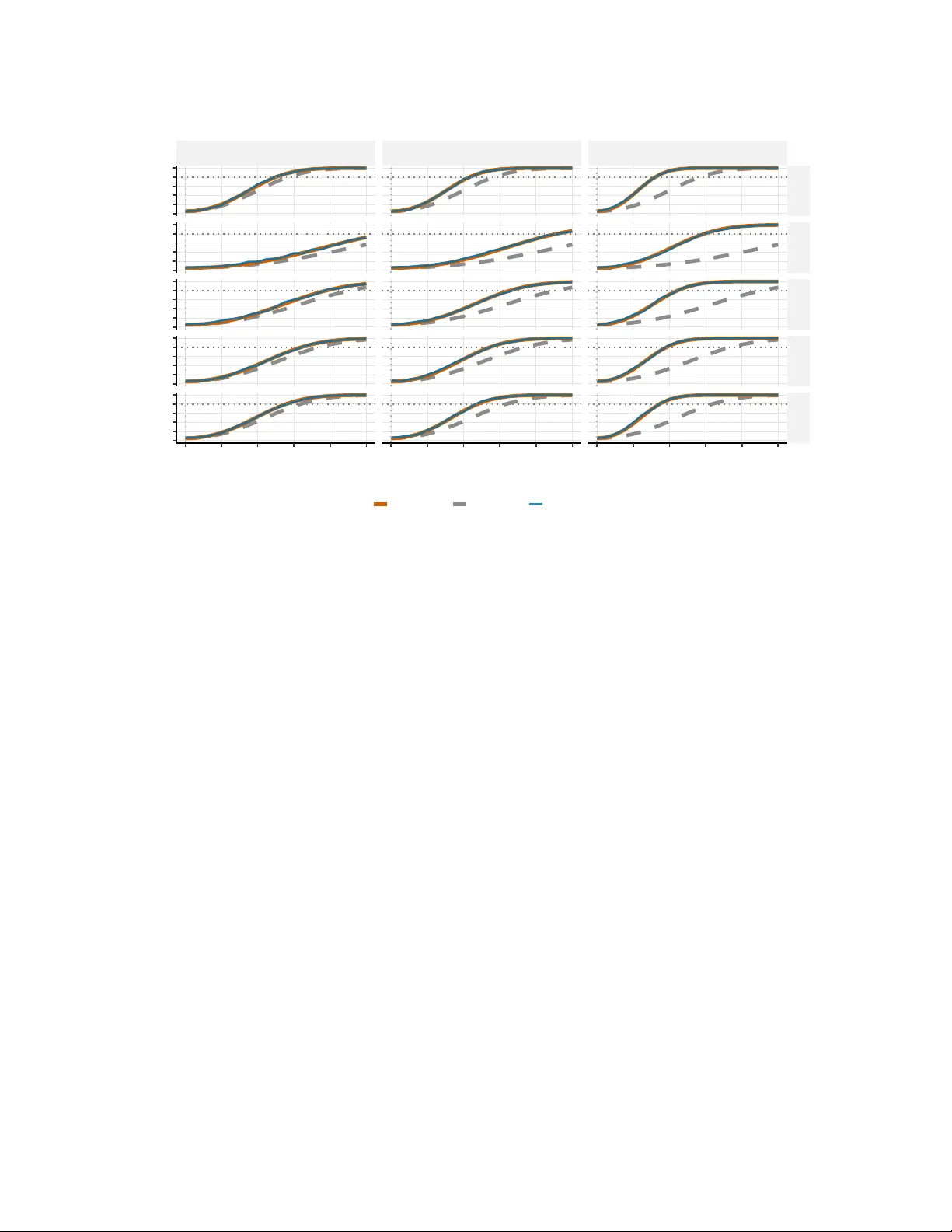
P o w er Analysis for Prediction-P o w ered Inference Yiqun T. Chen 1 , 2 , Moran Guo 1 , and Shengyi Li 1 1 Departmen t of Biostatistics, Johns Hopkins Univ ersity , Baltimore, Maryland 21205, U.S.A. 2 Departmen t of Computer Science, Johns Hopkins Univ ersit y , Baltimore, Maryland 21205, U.S.A. yiqun.t.chen@gmail.com Abstract Mo dern studies increasingly leverage outcomes predicted b y machine learning and artiﬁcial in telligence (AI/ML) mo dels, and recent work, suc h as prediction-p o w ered in- ference (PPI), has dev elop ed v alid do wnstream statistical inference procedures. How ever, classical p ow er and sample size form ulas do not readily accoun t for these predictions. In this w ork, w e tackle a simple yet practical question: giv en a new AI/ML mo del with high predictive p ow er, ho w man y labeled samples are needed to achiev e a desired lev el of statistical p o wer? W e deriv e closed-form p ow er form ulas b y c haracterizing the asymptotic v ariance of the PPI estimator and applying W ald test in version to obtain the required labeled sample size. Our results co ver widely used settings including t wo-sample comparisons and risk measures in 2 × 2 tables. W e ﬁnd that a useful rule of th um b is that the reduction in required lab eled samples relative to classical designs scales roughly with the R 2 b et ween the predictions and the ground truth. Our analytical form ulas are v alidated using Monte Carlo sim ulations, and w e illustrate the framew ork in three con temp orary biomedical applications spanning single-cell transcriptomics, clinical blo o d pressure measurement, and dermoscop y imaging. W e pro vide our softw are as an R pac k age and online calculators at https://github.com/yiqunchen/pppower . Keyw ords: Artiﬁcial in telligence; Exp erimental design; Lab el eﬃciency; P ow er analysis; Prediction-p o wered inference; Sample size. 1 In tro duction Gold-standard labels are fundamen tal for scien tiﬁc disco veries but remain time-consuming and exp ensiv e: Annotating cell t yp es in single-cell RNA-seq requires exp ert curation of mark er 1 genes [ Baron et al. , 2016 ]; measuring clinical outcomes in randomized trials demands patien t follo w-up and lab oratory assays [ Ro dger et al. , 2012 ]; and ev aluating the qualit y of large language mo del (LLM) resp onses to complex questions needs human exp ert judgmen ts [ Chiang et al. , 2024 ]. A t the same time, predictions from machine learning (ML) and artiﬁcial in telligence (AI) mo dels ha ve b ecome more accurate and a v ailable, where millions of cells can b e labeled in minutes, prognostic mo dels can score electronic health records at negligible cost, and “LLM-as-a-judge” pipelines, where an LLM serv es as the h uman exp ert, can ev aluate millions of resp onses in minutes. With the rise of these mo dels, it is natural to ask whether these predictions can reduce the n umber of costly lab els needed to answ er scientiﬁc questions of in terest, e.g., what is the prev alence of this disease or the c hange in cell-t yp e prop ortions across diﬀeren t exp erimen tal conditions. Recen t work has sho wn that treating predicted labels as direct observ ations is in v alid and inﬂates T yp e I error. Metho ds such as Pr e diction-Power e d Infer enc e (PPI) [ Angelopoulos et al. , 2023a ] and its tuned v arian t PPI++ [ Angelop oulos et al. , 2023b ] instead calibrate predictions against a small set of gold-standard labels. T ogether with related w ork [ Zrnic and Cand ` es , 2024 , Miao et al. , 2025 , Egami et al. , 2023 , Gronsb ell et al. , 2024 ], these metho ds yield un biased and asymptotically more eﬃcient estimators than classical analyses based on gold-standard lab els alone. Ho wev er, less work has translated those eﬃciency gains into the design-stage question ev ery study planner m ust answ er: Given a pr e dictive mo del’s ac cur acy, how many lab ele d samples ar e ne e de d to dete ct an eﬀe ct of inter est with the desir e d statistic al p ower? Classical p ow er form ulas [ Erdfelder et al. , 1996 , F aul et al. , 2007 ] do not provide a straigh tforward wa y to distinguish b etw een gold-standard lab els and predictions. As a result, practitioners either ignore predictions en tirely , whic h leads to v alid planning but p oten tial losses in eﬃciency , or naiv ely treat predictions as gold-standard lab els, whic h leads to o verestimated pow er and underestimated sample sizes. Sev eral recent con tributions start to address this gap: Angelop oulos et al. [ 2023b ] dev elop cost-allo cation routines from pilot data but do not pro vide closed-form p o wer or sample-size formulas. Comprehensiv e softw are pac k ages [ Salerno et al. , 2025 , Egami et al. , 2024 ] unify a range of p ost-prediction inference metho ds y et fo cus on the analysis stage and oﬀer no prosp ective study-design functionalit y . P oulet et al. [ 2025 ] deriv e p o w er reductions for ANCO V A-st yle regression adjustment but restrict attention to that single estimator. While most work fo cused on comparing asymptotic eﬃciency of estimators, Mani et al. [ 2025 ] also in vestigated the ﬁnite-sample trade-oﬀ, and our rule of th um b giv es that limitation a concrete planning in terpretation. Closest to our w ork is Brosk a et al. [ 2025 ], who in v ert the PPI++ v ariance form ula to join tly optimize the 2 lab eled and unlab eled sample sizes under a cost constrain t. Our starting p oin t diﬀers in a practical but imp ortan t w ay: in man y biomedical settings the t w o sample sizes are not join tly optimized. The p o ol of unlab eled observ ations is often ﬁxed b y the exp eriment itself (e.g., the num b er of cells captured in a single-cell assay , or the patients meeting inclusion criteria), and the binding constraint is ho w many a biologist or ph ysician can man ually lab el. W e therefore condition on a giv en N and ask ho w many gold-standard labels n are needed to ac hieve target p o wer. In this paper, we propose pppower , a framew ork and R pac k age for prediction-p o w ered p o wer analysis (see Figure 1 ). Our contributions are as follo ws: 1. Closed-form form ulas. W e deriv e pow er and sample-size form ulas for prediction- p o wered estimators that combine a smaller set of gold-standard lab els with a larger p o ol of mo del-based predicted labels, and show that they reduce to the classical form ulas when the predictions are uninformative. These formulas co ver t wo-sample comparisons, paired designs, o dds ratios and relativ e risks in 2 × 2 tables, and regression con trasts for (generalized) linear mo dels (Prop ositions 1 – 6 , 7 , and 8 ). A simple rule of th umb emerges: the required lab eled sample size drops b y approximately R 2 × 100%. 2. User-friendly parameterization. The formulas accept R 2 , sensitivity/speciﬁcity , or confusion matrices as inputs for the one-sample and binary-table designs, av oiding direct co v ariance sp eciﬁcation in the main op erational cases; regression-con trast extensions still require con trast-lev el pilot co v ariance blo cks (Sections 3.3 and 4.4 ). 3. Sim ulation v alidation. A comprehensive sim ulation study v alidates all formulas against Mon te Carlo estimates and establishes practical guidance on when mo del-based predicted lab els yield the largest reductions in required lab eled sample size (Section 5 ). 4. Op en-source soft w are with case study . An R pac k age with a pwr -st yle API and an accompan ying online calculator unify p ow er calculation and sample-size determination in a single function call. W e demonstrate the pac k age on three biomedical case studies (Section 6 ). 2 Setup and Bac kground W e consider i.i.d. lab eled data { ( X i , Y i ) } n i =1 dra wn from a join t distribution P X Y on X × Y , and an independent p o ol of unlabeled co v ariates { e X j } N j =1 dra wn from the same marginal P X , with r = n/ N denoting the lab eled-to-unlab eled ratio. Throughout, n denotes the 3 Y : true lab els, f : predictions, n : paired, N : predictions only Estimator ˆ θ λ = ¯ Y n + λ ( ¯ ˜ f N − ¯ f n ) P ow er and sample size in v ert V ar ( ˆ θ λ ) to obtain required labels n ⋆ (a) Estimator-and-inv ersion sc hematic. 140 150 160 170 180 500 1,000 2,000 Unlabeled pool N Planned labeled n* Classical Age only Clinical LM Clinical RF (b) NHANES planning b y surrogate mo del. Figure 1: Prediction-p ow ered planning. Panel (a) shows the notation, estimator, and v ariance in version. P anel (b) sho ws the NHANES sample-size plan for ∆ = 4 mmHg: gray is the classical design, and the orange curv es are the age-only linear model, the richer clinical linear mo del, and the random forest surrogate. n umber of gold-standard lab els and N the size of the larger unlab eled sample carrying mo del-based predictions, with the practically important regime often ha ving N ≫ n . A predictor f : X → Y yields predictions f i = f ( X i ) on lab eled observ ations and e f j = f ( e X j ) on unlab eled ones; w e treat f as indep enden t of b oth samples (e.g., a pre-trained mo del), and note that cross-ﬁtting can relax this assumption in practice (see the Supplemen tary Material and Zrnic and Cand` es [ 2024 ]). Bey ond σ 2 Y = V ar ( Y ), three second-order quan tities go vern the in terplay b etw een outcomes and predictions throughout the pap er. The prediction v ariance σ 2 f = V ar ( f ( X )) and the residual v ariance σ 2 ε = V ar ( Y − f ( X )) = σ 2 Y + σ 2 f − 2 Co v ( Y , f ) together measure how m uch v ariation in Y the predictor captures; the outcome–prediction correlation ρ Y f = Co v ( Y , f ) / ( σ Y σ f ) summarizes this in a single unitless quan tit y , with ρ 2 Y f equal to the fraction of σ 2 Y explained b y f . Finally , we deﬁne the v ariance threshold S 2 = n ∆ / ( z 1 − α/ 2 + z 1 − β ) o 2 . (1) 2.1 T esting for One-Sample Mean W e ﬁrst consider testing equality of the population mean θ ⋆ = E [ Y ]: H 0 : θ ⋆ = θ 0 v ersus H 1 : θ ⋆ = θ 0 + ∆ , (2) 4 at signiﬁcance level α with target p ow er 1 − β . The sample mean ¯ Y = n − 1 P n i =1 Y i is unbiased for θ ⋆ with v ariance σ 2 Y /n . The p ow er of the tw o-sided W ald test for ( 2 ) is P ow er cl ( n ) = Φ  − z 1 − α/ 2 + | ∆ | σ Y / √ n  + Φ  − z 1 − α/ 2 − | ∆ | σ Y / √ n  . (3) In verting ( 3 ) b y dropping the negligible second term gives n cl ≥ σ 2 Y /S 2 . F or ﬁxed α , β , and ∆, σ 2 Y is the only determinan t of the required sample size: reducing it is the only wa y to increase p o w er for a ﬁxed n . 2.2 Recap of Prediction-P o w ered Inference The classical p ow er formula in ( 3 ) cannot directly make use of the predictions ˜ f . In this section, w e ﬁrst review the PPI and PPI++ estimators and their v ariances, whic h can then b e in verted to obtain the p o wer form ulas using b oth gold-standard lab els and predictions. When the p opulation mean is the target of interest, the PPI estimator [ Angelop oulos et al. , 2023a ] mak es a simple observ ation that the p opulation mean decomp oses as θ ⋆ = E [ f ( X )] + E [ Y − f ( X )], and eac h comp onen t can b e estimated separately: b θ PPI = 1 N N X j =1 e f j | {z } unlabeled mean + 1 n n X i =1 ( Y i − f i ) | {z } labeled correction . (4) Prop osition 1 (Mean PPI++ v ariance) Under our setup, the PPI estimator is unbiase d and asymptotic al ly normal with varianc e V ar( b θ PPI ) = σ 2 f N + σ 2 ε n . (5) The two terms r eﬂe ct pr e diction noise σ 2 f / N fr om the unlab ele d sample and r esidual noise σ 2 ε /n fr om the lab ele d sample. When N is lar ge, the varianc e is dominate d by σ 2 ε /n . While PPI in ( 4 ) uses f i , the r esulting estimator r emains unbiase d if we r eplac e f i with any function g ( f i ) , and an appr opriate choic e of g c ould further r e duc e the varianc e. PPI++ [ A ngelop oulos et al. , 2023b ] c onsiders g ( f i ) = λf i with a tunable p ar ameter λ ∈ R c ontr ol ling the weight plac e d on pr e dictions: b θ λ = n − 1 n X i =1 Y i + λ ( N − 1 N X j =1 e f j − n − 1 n X i =1 f i ) . (6) 5 The asymptotic varianc e of b θ λ is V ar( b θ λ ) = σ 2 Y n + λ 2 σ 2 f  1 N + 1 n  − 2 λ Co v ( Y , f ) n , (7) and the asymptotic-varianc e-minimizing tuning p ar ameter is λ ⋆ = Co v ( Y , f ) (1 + r ) σ 2 f , (8) with r esulting optimal varianc e V ar( b θ λ ⋆ ) = σ 2 Y n − Co v ( Y , f ) 2 σ 2 f · N n ( n + N ) . (9) 3 P o w er and Sample Size for PPI++ Since PPI is the sp ecial case of PPI++ with λ = 1, w e state all results for general λ ; setting λ = 1 reco vers the PPI-speciﬁc results. The optimal v ariance ( 9 ) pla ys the same role for PPI++ that σ 2 Y /n pla ys for the classical estimator: it determines the p o w er of the W ald test. 3.1 T ests for a One-Sample Mean Prop osition 2 ( PPI++ p o wer) Consider testing ( 2 ) using the Wald statistic Z = ( b θ λ ⋆ − θ 0 ) / q V ar( b θ λ ⋆ ) . R e c al ling V ar( b θ λ ⋆ ) fr om ( 9 ) , the p ower of the two-side d test at level α is P ow er PPI ( n, N ) = Φ   − z 1 − α/ 2 + | ∆ | q V ar( b θ λ ⋆ )   + Φ   − z 1 − α/ 2 − | ∆ | q V ar( b θ λ ⋆ )   . (10) In verting ( 10 ) b y setting V ar ( b θ λ ⋆ ) ≤ S 2 and solving the resulting quadratic in n yields the follo wing sample-size form ula. Prop osition 3 ( PPI++ sample size) The minimum lab ele d sample size r e quir e d to achieve p ower 1 − β is n ≥ σ 2 Y − S 2 N + q ( σ 2 Y − S 2 N ) 2 + 4 S 2 N σ 2 Y (1 − ρ 2 Y f ) 2 S 2 . (11) W e write n ⋆ for the smallest in teger lab eled sample size satisfying ( 11 ) , that is, the in verted minim um num b er of gold-standard lab els needed to attain the target p ow er. F or 6 ﬁxed N , the in version in ( 11 ) can return n ⋆ > N . This do es not in v alidate the v ariance form ula; it simply means that a ﬁxed-p o ol design would exhaust the av ailable prediction p o ol. Suc h a regime may be of limited practical interest, as the motiv ating assumption is that the main constrain t lies in the cost of obtaining gold-standard lab els. Corollary 4 (Rule of thum b) In the r e gime N ≫ n , the term σ 2 f / N b e c omes ne gligible and the optimal varianc e r e duc es to V ar ( b θ λ ⋆ ) ≈ σ 2 Y (1 − ρ 2 Y f ) /n , yielding the simple appr oximation n PPI /n cl ≈ 1 − ρ 2 Y f . Rule of th um b. A predictor with R 2 = ρ 2 Y f reduces the required lab eled sample size b y appro ximately R 2 × 100%. F or example, R 2 = 0 . 5 halv es the lab eled-data requirement, and R 2 = 0 . 9 yields up to a 90% reduction. 3.2 Connection to Semiparametric Eﬃciency The family of estimators n − 1 P n i =1 Y i − n − 1 P n i =1 g ( f i ) + N − 1 P N j =1 g ( e f j ) is unbiased for θ ⋆ for an y function g , and the c hoice of g go verns the asymptotic v ariance. F or the mean functional, c ho osing g ( f ) = E [ Y | f ] minimizes the asymptotic v ariance not merely within this family but among all asymptotically un biased estimators of θ ⋆ , a direct consequence of classical semiparametric eﬃciency theory . In this one-sample mean setting, the factor 1 − ρ 2 Y f in the rule of th um b ab o ve represen ts the fundamental limit on ho w muc h predictions can help: it is the eﬃciency b ound, not just the p erformance of a particular estimator. In the sp ecial case where Y and f ( X ) are b oth binary , the linear construction with optimal λ ac hieves this b ound, so PPI++ is semiparametrically eﬃcient. In more general settings the linear form may be sub optimal [ Chen et al. , 2026 , Ji et al. , 2025 , Xu et al. , 2025 , Song et al. , 2026 ], and the v ariance-optimal estimator could replace λf i with a non-linear estimate b g ( f i ) of E [ Y | f ], whic h can b e estimated from the labeled data. In this case, the same set of arguments holds but the estimated v ariance will diﬀer. 3.3 Calibration from Common Metrics F or the one-sample mean form ulas abov e, the prediction en ters through Co v ( Y , f ) 2 /σ 2 f = σ 2 Y ρ 2 Y f , so the k ey planning inputs reduce to the outcome v ariance σ 2 Y and the squared outcome–prediction correlation ρ 2 Y f . In practice, how ev er, ML mo del do cumentation does not alw ays report these quan tities directly: con tinuous models are typically summarized b y held-out R 2 , while classiﬁers are c haracterized by metrics such as accuracy , precision, and recall. 7 Con tinuous outcomes. When the model R 2 is reported in prior publications, w e can use R 2 = ρ 2 Y f directly . Man y soft ware pac k ages instead rep ort the mean-squared error σ 2 ε = σ 2 Y + σ 2 f − 2 Co v ( Y , f ). This summary do es not identify σ 2 f and Co v ( Y , f ) separately , but it still giv es a conserv ative planning input: b y Cauch y–Sc h warz, σ 2 ε ≥ σ 2 Y (1 − ρ 2 Y f ), so R 2 ≤ ρ 2 Y f . Thus plugging suc h an R 2 in to the rule of thum b, or into ( 11 ) through ρ 2 Y f ≈ R 2 , will giv e us a more conserv ativ e estimate of the num b er of required samples. Binary outcomes. F or a binary outcome Y ∈ { 0 , 1 } and a binary classiﬁer f ∈ { 0 , 1 } , the required v ariance components are determined b y three quan tities: the outcome prev alence p = P ( Y = 1), the sensitivity se = P ( f = 1 | Y = 1) and the sp eciﬁcit y sp = P ( f = 0 | Y = 0). F rom these, the prediction prev alence is p f = se · p + (1 − sp )(1 − p ), and the three inputs follo w as σ 2 Y = p (1 − p ), σ 2 f = p f (1 − p f ), and Co v( Y , f ) = se · p − p · p f . 4 Extensions to Other Designs W e next extend the one-sample framew ork of Section 3 to other commonly used designs: t wo-sample comparisons (unpaired and paired), 2 × 2 table tests, and contrasts for linear and logistic mo dels. 4.1 T ests for Equalit y of Tw o Means Consider comparing t wo indep endent groups A and B with p opulation means θ ⋆ A and θ ⋆ B , where the parameter of in terest is θ ⋆ A − θ ⋆ B . F or eac h group g ∈ { A, B } , w e observ e n g lab eled pairs and N g unlab eled observ ations, and construct a group-speciﬁc PPI++ estimator b θ g , PPI as in ( 6 ). The PPI++ estimator of the group diﬀerence is b ∆ PPI = b θ A, PPI − b θ B , PPI . (12) Prop osition 5 (Two-sample PPI++ v ariance) Under indep endent gr oups, the varianc e of b ∆ PPI at the gr oup-sp e ciﬁc or acle tuning p ar ameters is V ar( b ∆ PPI ) = X g ∈{ A,B } " σ 2 Y ,g n g − Co v ( Y g , f g ) 2 σ 2 f ,g · N g n g ( n g + N g ) # . (13) In the r e gime N A , N B ≫ n A , n B , this r e duc es to V ar( b ∆ PPI ) ≈ σ 2 Y ,A  1 − Corr( Y A , f A ) 2  n A + σ 2 Y ,B  1 − Corr( Y B , f B ) 2  n B , (14) 8 which is the sum of the gr oup-sp e ciﬁc one-sample varianc es, e ach r e duc e d by the squar e d outc ome–pr e diction c orr elation within that gr oup. The required sample sizes n A and n B follo w from setting V ar ( b ∆ PPI ) ≤ S 2 from ( 1 ) and sp ecifying an allo cation ratio n A /n B ; for a balanced design ( n A = n B = n ) the condition b ecomes n ≥ [ σ 2 Y ,A (1 − Corr( Y A , f A ) 2 ) + σ 2 Y ,B (1 − Corr( Y B , f B ) 2 )] /S 2 . 4.2 T ests for P aired Mean Diﬀerences In paired designs, eac h sub ject i con tributes measurements under b oth conditions (e.g., b efore and after treatmen t), yielding within-sub ject diﬀerences Y A i − Y B i with paired predictions f A ( X i ) − f B ( X i ). The parameter of in terest is E [ Y A − Y B ], and the problem reduces directly to the one-sample framewor k applied to the diﬀerences. Prop osition 6 (Paired PPI++ v ariance) L et D i = Y A i − Y B i and G i = f A i − f B i . Applying the one-sample PPI++ r esult to the p air e d diﬀer enc es gives V ar( b ∆ PPI++ ) = V ar( D ) n − Co v ( D , G ) 2 V ar( G ) · N n ( n + N ) = V ar( D ) n  1 − Corr( D , G ) 2 N n + N  . When N ≫ n , this b e c omes V ar ( b ∆ PPI++ ) ≈ V ar ( Y A − Y B ) { 1 − Corr ( Y A − Y B , f A − f B ) 2 } /n . Just as a paired design can be more eﬃcien t than an unpaired t w o-sample test b y remo ving b et ween-sub ject noise, the correlation Corr ( Y A − Y B , f A − f B ) go verns the eﬃciency gain here and can diﬀer substan tially from the marginal correlations Corr ( Y A , f A ) and Corr ( Y B , f B ): if the predictor captures within-sub ject v ariation well, this correlation can be high ev en when the marginal correlations are mo derate, and conv ersely . 4.3 T ests for Relativ e Risk and Odds Ratio in 2 × 2 T ables Man y clinical and epidemiological studies compare whether a binary even t o ccurs in t wo groups, suc h as treatmen t ( g = 1) and con trol ( g = 0). F or eac h group g , the labeled data con tain ev ent indicators Y g i ∈ { 0 , 1 } , while the prediction mo del pro duces a surrogate f g ( X ) for that same ev ent indicator on b oth the lab eled and unlab eled sub jects in that group. This setup is often summarized as a 2 × 2 table of aggregated coun ts indexed b y the group lab el g and the outcome Y . The t w o standard eﬀect measures in this setting are RR = p 1 p 0 , OR = p 1 / (1 − p 1 ) p 0 / (1 − p 0 ) , and under the n ull h yp othesis that the treatment g has no eﬀect, we would hav e RR = OR = 1. In 9 practice, w e often consider the equiv alen t formulation on the log scale using log ( RR ) = log p 1 − log p 0 and log(OR) = logit( p 1 ) − logit( p 0 ). As b oth estimands only depend on the group-sp eciﬁc ev ent probabilit y p g = P ( Y = 1 | G = g ), it suﬃces to estimate p g using b p g ,λ g = ¯ Y L,g + λ g ( ¯ f U,g − ¯ f L,g ). Here, ¯ Y L,g is the labeled ev ent rate, and ¯ f L,g and ¯ f U,g are the av erage predictions in the labeled and unlabeled samples from group g . Under our indep endence assumption, the asymptotic v ariance of log c RR and log d OR follo ws directly from the delta metho d. Prop osition 7 ( PPI++ sample size for relativ e risk and o dds ratio) Assume the two gr oups ar e indep endent, let ρ g = Corr ( Y g , f g ) , and ﬁx an al lo c ation r atio κ = n 1 /n 0 . In the r e gime N g ≫ n g , deﬁne ∆ RR = log ( p 1 /p 0 ) , ∆ OR = logit ( p 1 ) − logit ( p 0 ) , S 2 RR = ∆ 2 RR / ( z 1 − α/ 2 + z 1 − β ) 2 , and S 2 OR = ∆ 2 OR / ( z 1 − α/ 2 + z 1 − β ) 2 . Then V ar(log c RR) ≈ 1 n 0  (1 − p 0 )(1 − ρ 2 0 ) p 0 + 1 κ (1 − p 1 )(1 − ρ 2 1 ) p 1  , V ar(log d OR) ≈ 1 n 0  1 − ρ 2 0 p 0 (1 − p 0 ) + 1 κ 1 − ρ 2 1 p 1 (1 − p 1 )  . Conse quently, the minimum lab ele d sample sizes r e quir e d for a two-side d Wald test at level α with p ower 1 − β ar e n RR 0 ≥ 1 S 2 RR  (1 − p 0 )(1 − ρ 2 0 ) p 0 + 1 κ (1 − p 1 )(1 − ρ 2 1 ) p 1  , n RR 1 = κn RR 0 , n OR 0 ≥ 1 S 2 OR  1 − ρ 2 0 p 0 (1 − p 0 ) + 1 κ 1 − ρ 2 1 p 1 (1 − p 1 )  , n OR 1 = κn OR 0 . F or b alanc e d designs, set κ = 1 . Setting ρ 0 = ρ 1 = 0 r e c overs the classic al r elative-risk and o dds-r atio sample-size formulas. 4.4 T ests for Regression Con trasts in Generalized Linear Mo dels Man y of the p ow er analyses ab ov e can b e recast as testing a linear contrast in a generalized linear mo del. W e ﬁrst motiv ate prediction-p ow ered inference for linear mo dels. Consider the ordinary least squares (OLS) estimator with target co eﬃcient v ector β ⋆ that minimizes E [( Y − X ⊤ β ) 2 ]. The normal equations imply E [ X X ⊤ ] β ⋆ = E [ X Y ]. No w, for cov ariate–outcome observ ation pairs ( x i , y i ), if f ( x i ) is a prediction of y i , w e can decomp ose the normal equation as E [ X Y ] = E [ X f ( X )] + E [ X { Y − f ( X ) } ] , whic h leads to 10 the estimating equation 1 n n X i =1 X i  Y i − X ⊤ i β  + λ " 1 N N X j =1 e X j  e f j − e X ⊤ j β  − 1 n n X i =1 X i  f i − X ⊤ i β  # = 0 . Similarly , for a generalized linear mo del with mean function µ β ( X ), the target parameter satisﬁes the score equation E [ X { Y − µ β ( X ) } ] = 0 at β = β ⋆ , motiv ating the decomp osition E [ X { Y − µ β ( X ) } ] = E [ X { µ f ( X ) − µ β ( X ) } ] + E [ X { Y − µ f ( X ) } ] , whic h yields the analogous PPI++ score equation 1 n n X i =1 X i  Y i − µ β ( X i )  + λ " 1 N N X j =1 e X j  µ f ( e X j ) − µ β ( e X j )  − 1 n n X i =1 X i  µ f ( X i ) − µ β ( X i )  # = 0 . With r = n/ N , a ﬁrst-order expansion of b θ λ giv es V ar( b θ λ ) ≈ V Y Y + λ 2 (1 + r ) V f f − 2 λV Y f n , where V Y Y , V f f , and V Y f denote the con trast-level v ariances of the lab eled score term, the prediction term, and their cov ariance. Belo w, in Prop osition 8 , w e summarize the p o wer and required sample size for the contrast of in terest θ ⋆ = a ⊤ β ⋆ using the PPI++ estimator. Prop osition 8 ( PPI++ sample size for regression contrasts) L et ∆ = a ⊤ β ⋆ denote the tar get c ontr ast under the alternative. The or acle tuning p ar ameter is λ ⋆ = V Y f / { (1 + r ) V f f } , which yields V ar( b θ λ ⋆ ) ≈ 1 n  V Y Y − V 2 Y f (1 + r ) V f f  . T r e ating N as ﬁxe d, the minimum lab ele d sample size r e quir e d for a two-side d Wald test at level α with p ower 1 − β satisﬁes n ≥ V Y Y − S 2 N + r ( V Y Y − S 2 N ) 2 + 4 S 2 N  V Y Y − V 2 Y f V f f  2 S 2 . In the r e gime N ≫ n , this simpliﬁes to n ≥ V Y Y − V 2 Y f /V f f S 2 . 11 5 Sim ulation Studies Here, w e v alidate the appro ximate closed-form form ulas deriv ed in Sections 3 – 4 through comprehensiv e Mon te Carlo sim ulations. F or each scenario, w e generate R = 1 , 000 replicates and compare the empirical p ow er of the PPI++ -based tests with the theoretical form ulas w e presented. Unless otherwise noted, all tests are t w o-sided at level α = 0 . 05 and use the oracle λ ⋆ , and we target a pow er of 80% in the sample size calculations. W e also examine sev eral robustness c hec ks, including whether the PPI++ -based tests hav e the correct size (i.e., con trol T yp e I error at the nominal level), the discrepancy b etw een the estimated and oracle v alues of λ ⋆ , and departures from the normalit y assumptions (e.g., small n or non-normal outcomes). W e present the main p ow er and sample size v alidation results in the main text, with additional robustness ch ec ks deferred to the Supplemen tary Material. 5.1 P o w er V alidation Mean estimation. W e consider b oth contin uous and binary outcomes. F or the contin uous case, we sim ulate ( Y , f ) as biv ariate normal with σ 2 Y = σ 2 f = 1, correlation ρ ∈ { 0 . 5 , 0 . 7 , 0 . 9 } , and ( n, N ) ∈ { 20 , 40 , 60 , 80 , 100 } × { 200 , 500 } , with a target eﬀect size of ∆ = 0 . 2. F or the binary outcome exp erimen t, w e generate outcomes Y ∼ Bernoulli ( p = 0 . 3) with predictions generated via sensitivit y and sp eciﬁcit y conditional on Y , and ∆ = 0 . 05. Across b oth settings, pow er increases as the predictiv e accuracy of the lab els increases (higher ρ ) and as the n um b er of lab eled samples ( n ) increases, and there is strong agreemen t b et ween the theoretical and empirical p o wer (Figure 2 ). F or binary outcomes, the analytical appro ximation captures the ov erall trend, but the smallest- n , highest-accuracy settings sho w visible ﬁnite-sample departures (e.g., sensitivity = sp eciﬁcity = 0 . 95, N = 500, n = 20). Our p ow er planning form ula is mildly optimistic (ab out 10% inﬂation), primarily due to instabilit y in the estimated denominator at v ery small n . Tw o-sample tests. W e simulate indep endent groups with contin uous (∆ = 0 . 3) and binary (∆ = 0 . 08) outcomes using the same parameter grids as in the mean estimation exp erimen ts. Across both outcome types, the theoretical curv es trac k the empirical p ow er closely o ver the full ( n, N ) grid, with maxim um absolute discrepancies of 0.02 and 0.03 for con tinuous and binary outcomes, respectively . The largest deviations typically occur in the most prediction-fa vorable regimes with v ery small lab eled samples, where the denominator in the estimated v ariance of the W ald test is again the main source of extra v ariabilit y . See Figures S1 – S2 in the Supplementary Material. 12 ρ = 0.5 ρ = 0.7 ρ = 0.9 N = 200 N = 500 20 40 60 80 100 20 40 60 80 100 20 40 60 80 100 0.0 0.2 0.4 0.6 0.8 1.0 0.0 0.2 0.4 0.6 0.8 1.0 Labeled Sample Size (n) P ower Analytical Classical Empirical Mean Estimation (Continuous) (a) Gaussian outcomes. Sens/Spec = 70% Sens/Spec = 85% Sens/Spec = 95% N = 200 N = 500 25 50 75 100 25 50 75 100 25 50 75 100 0.0 0.2 0.4 0.6 0.8 1.0 0.0 0.2 0.4 0.6 0.8 1.0 Labeled Sample Size (n) P ower Analytical Classical Empirical Mean Estimation (Binary) (b) Binary outcomes. Figure 2: One-sample mean v alidation: empirical p o wer (points, with 95% Mon te Carlo error bars for the binary setting) versus theoretical pow er (lines) for PPI++ with oracle λ ⋆ . P aired designs. P aired con tinuous and binary designs with within-pair prediction correla- tion sho w the same o v erall pattern of strong agreemen t b etw een theoretical and empirical p o wer (see Figures S3 – S4 ), with the largest gaps again app earing at small n . These results suggest that the paired-design appro ximation remains accurate once the within-pair co v ariance structure is accoun ted for. 13 Accuracy = 70% Accuracy = 80% Accuracy = 90% N = 200 N = 500 20 40 60 80 100 20 40 60 80 100 20 40 60 80 100 0.0 0.2 0.4 0.6 0.8 1.0 0.0 0.2 0.4 0.6 0.8 1.0 T otal Labeled Sample Size (n) P ower Analytical Classical Empirical 2x2 T able: Odds Ratio Accuracy = 70% Accuracy = 80% Accuracy = 90% N = 200 N = 500 20 40 60 80 100 20 40 60 80 100 20 40 60 80 100 0.0 0.2 0.4 0.6 0.8 1.0 0.0 0.2 0.4 0.6 0.8 1.0 T otal Labeled Sample Size (n) P ower Analytical Classical Empirical 2x2 T able: Relative Risk Figure 3: Odds-ratio and relative-risk v alidation in 2 × 2 tables—analytical (lines) versus empirical (p oints) PPI++ p o wer for o dds ratio (top) and relative risk (b ottom). Dashed lines sho w classical p o wer. 5.2 Extensions: 2 × 2 T ables and Generalized Linear Mo dels W e next v alidate the con tingency-table and regression extensions dev elop ed in Section 4 . 2 × 2 table (o dds ratio and relativ e risk). The data-generating pro cess dra ws binary treatmen t X ∈ { 0 , 1 } and binary outcome Y with control probability p ctrl = 0 . 20 and exp erimen tal probabilit y p exp ∈ { 0 . 30 , 0 . 35 , 0 . 40 } . A noisy binary classiﬁer with sensitivit y = sp eciﬁcit y = accuracy serves as the surrogate, with accuracy ∈ { 70% , 80% , 90% } . Figure 3 displa ys the p ow er result for p exp = 0 . 40, whic h corresp onds to a relativ e risk of 2 . 00 and o dds ratio of 2 . 67; agreement is generally tigh t. 14 Linear regression con trast. W e sim ulate X ∼ N (0 , I 2 ), Y = X β + ε with β = (∆ , 0), ∆ = 0 . 3, and predictions f = X β + ν where ν = ρ ε + p 1 − ρ 2 η , η ∼ N (0 , 1). The con trast a = (1 , − 1) tests H 0 : β 1 − β 2 = 0. Under this sim ulation setting, V ar ( a ⊤ β ) in Prop osition 8 reduces to V Y Y = 2, V f f = 2, and V Y f = 2 ρ . Each Mon te Carlo replicate constructs the PPI++ estimator with oracle λ ⋆ and a sandwich estimator for the standard error, then p erforms a tw o-sided W ald test. Figure 4 (a) shows close agreemen t across all 30 conﬁgurations ( n ∈ { 20 , 40 , 60 , 80 , 100 } , N ∈ { 200 , 500 } , ρ ∈ { 0 . 5 , 0 . 7 , 0 . 9 } ); the maxim um discrepancy is 0.08 at small n where ﬁnite-sample sandwich bias is exp ected. Logistic regression con trast. W e extend to non-linear mo dels b y sim ulating X ∼ N (0 , I 2 ), P ( Y = 1 | X ) = expit ( X β ) with β = (0 . 5 , 0) (corresponding to an o dds ratio of e 0 . 5 ≈ 1 . 65). W e consider a noisy binary classiﬁer with sensitivit y = speciﬁcity = accuracy as the surrogate. Because the required con trast-level v ariance blo c ks do not admit con venien t closed forms for logistic regression, w e appro ximate the corresponding population quantities once using a large Mon te Carlo reference sample ( M = 100 , 000) and use them to ev aluate the analytical p o wer curv e. F or the empirical p ow er calculation, each fresh simulated dataset estimates a tw o-fold cross-ﬁtted plug-in tuning parameter ˆ λ and then solves the corresp onding rectiﬁed score equation using that plug-in estimate. Figure 4 (b) displays results across 30 conﬁgurations ( n ∈ { 20 , 40 , 60 , 80 , 100 } , N ∈ { 200 , 500 } , accuracy ∈ { 70% , 80% , 90% } ); the maxim um discrepancy is 0.1, concentrated at small n with high accuracy where estimating ˆ λ adds the most ﬁnite-sample v ariabilit y . 5.3 Robustness Chec ks W e also examine sample-size in version accuracy , T yp e I error con trol of the PPI++ tests, and departures from Gaussian assumptions. Fixing target p ow er in { 0 . 60 , 0 . 70 , 0 . 80 , 0 . 90 } sho ws that the planned in teger sample size n ⋆ deliv ers achiev ed p ow er close to target across the one-sample, t wo-sample, and paired designs; analytical deviations are uniformly small, and empirical deviations are only mo dest in the smallest- n cells (Figure S5 in the Supplemen tary Material). W e also veriﬁed that, under the n ull, rejection rates remain close to the nominal 0 . 05 level, ranging from 0 . 04 to 0 . 06 in the con tin uous and binary settings (Figure S7 in the Supplemen tary Material). Moreo ver, with N = 1 , 000 ﬁxed, the plug-in estimate of the tuning parameter ˆ λ con verges steadily to w ard the oracle λ ⋆ as n gro ws (Figure S8 in the Supplemen tary Material). W e next stress the formulas through practical implemen tation choices and ﬁnite-sample p erturbations around the Gaussian b enc hmark. Replacing the oracle tuning parameter b y the plugin estimate ˆ λ c hanges p ow er v ery little on the Gaussian one-sample settings: the 15 ρ = 0.5 ρ = 0.7 ρ = 0.9 N = 200 N = 500 20 40 60 80 100 20 40 60 80 100 20 40 60 80 100 0.0 0.2 0.4 0.6 0.8 1.0 0.0 0.2 0.4 0.6 0.8 1.0 Labeled Sample Size (n) P ower Analytical Classical Empirical OLS Regression Contrast (a) OLS b eta-co eﬃcien t contrast v alidation. Accuracy = 70% Accuracy = 80% Accuracy = 90% N = 200 N = 500 20 40 60 80 100 20 40 60 80 100 20 40 60 80 100 0.0 0.2 0.4 0.6 0.8 1.0 0.0 0.2 0.4 0.6 0.8 1.0 Labeled Sample Size (n) P ower Analytical Classical Empirical (cross−fitted plugin) GLM Logistic Regression Contrast (b) Logistic-regression con trast v alidation. Figure 4: Regression-con trast v alidation: analytical (lines) versus empirical (p oints) PPI++ p o wer. In panel (b), the empirical logistic-regression p oin ts use a t w o-fold cross-ﬁtted plug-in ˆ λ estimated within eac h replicate, while the analytical curve uses the large-reference-sample appro ximation. Dashed lines sho w the corresp onding classical p ow er curv es. maxim um oracle–plugin diﬀerence is 0 . 03, and both remain close to the analytical curv e (Figure S9 in the Supplemen tary Material). A sweep o ver eﬀect size ∆ ∈ [0 , 0 . 5] at ﬁxed N = 500 pro duces the expected S-shap ed pow er curv es, with larger ρ shifting the PPI++ curv es left ward (Figure S10 in the Supplemen tary Material). Pushing the Gaussian one-sample design down to n ∈ { 15 , 20 , 25 , 30 , 50 , 100 } sho ws that the appro ximation remains usable but is predictably weak est b elow about n = 25 (Figure S11 in the Supplemen tary Material), 16 while v arying N /n from 1 to 100 at ﬁxed n = 50 sho ws that gains from unlab eled data rise quic kly and then saturate around N /n ≈ 10–20 (Figure S12 in the Supplementary Material). F or t wo-sample designs with ﬁxed total lab eled and unlab eled budgets, balanced allo cation remains b est and the analytical curves con tinue to trac k the empirical results closely across im balance ratios (Figure S13 in the Supplemen tary Material). Finally , w e rerun the one-sample mean exp erimen ts under tw o non-Gaussian outcome distributions on the same ( n, N , ρ ) grid. F or t 5 outcomes, agreemen t with the Gaussian-based form ula remains tight, with a maxim um discrepancy of 0 . 02. F or log-normal outcomes, the approximation remains reasonable once n is mo derate, but the most skew ed, small- n conﬁgurations show visibly larger departures, with a maximum discrepancy of 0 . 14. This suggests that mo derate hea vy tails alone are less problematic, whereas small samples com bined with strong sk ewness can p ose challenges for accurate pow er planning. 6 Real Data Applications In this section, w e illustrate the p o wer-analysis w orkﬂow on three biomedical datasets: cell- t yp e classiﬁcation in single-cell RNA-seq [ Baron et al. , 2016 ], blo o d pressure estimation in NHANES 2017–2018 [ Cen ters for Disease Control and Prev ention (CDC). National Center for Health Statistics (NCHS) , 2020 ], and melanoma detection in ISIC 2020 dermoscopy images [ Rotem b erg et al. , 2021 ]. F or each dataset, w e split the observed data in to training, pilot, and ev aluation subsets. The prediction mo dels f are ﬁt on the training split to mimic a pretrained mo del; the pilot split provides the v ariance and co v ariance inputs used to plan the lab eled sample size n ⋆ ; and the ev aluation split is treated as an empirical population with full-data truth θ ev al . Within eac h application, we sp ecify a target eﬀect size ∆ and set the n ull v alue to θ 0 = θ ev al − ∆, so the held-out ev aluation split serves as the alternative truth. In all three applications w e allo cate 25% of the observed data to training, 15% to the pilot split, and the remaining 60% to held-out ev aluation. This keeps the pilot meaningfully smaller than the analysis p opulation while still lea ving enough data to estimate the planning inputs. F or ISIC, where m ultiple images come from the same patient, this split is done at the patien t lev el to av oid leak age across rep eated lesions. Throughout this section, all designs target p o wer 0 . 80 at level α = 0 . 05. Achiev ed p o w er is estimated empirically from 500 held-out resamples: for the classical design we repeatedly draw n cl lab eled observ ations from the ev aluation split, while for PPI++ w e dra w n ⋆ lab eled observ ations together with N additional unlab eled observ ations from the remaining held-out units, apply the corresp onding test of H 0 : θ = θ 0 , and record the rejection rate. 17 6.1 Cell-T yp e Classiﬁcation in Single-Cell RNA-Seq Baron et al. [ 2016 ] constructed a pancreas scRNA-seq atlas that proﬁles pancreatic cell types across donors. W e fo cus on a simple comp osition question: among alpha and b eta cells, ho w diﬀerent are their population shares? Restricting atten tion to those t wo cell t yp es, the target estimand is θ = p β − p α , the diﬀerence in cell-t yp e prop ortions. The cov ariates X are the cell-lev el gene-expression proﬁles used to predict cell iden tity . W e split the 4 , 851 b eta-or-alpha cells into 1 , 212 training cells, 727 pilot cells, and 2 , 912 ev aluation cells. In the ev aluation split, p β = 0 . 521 and p α = 0 . 479, giving θ ev al = 0 . 041. T o create a meaningful gradient of prediction qualit y , w e compare three prediction rules trained on the training split: a delib erately w eak donor-only logistic mo del that uses only donor iden tit y , a one-gene logistic mo del using INS expression from the Baron data itself, and a random forest ﬁt on the top 20 mark er genes ranked within the training split b y diﬀeren tial mean log-expression b etw een b eta and alpha cells rather than imp orted from an external mark er database. The pilot split is used to estimate the corresp onding ρ 2 Y f v alues and to plan the lab eled sample size for ∆ = 0 . 10 and N ∈ { 500 , 1 , 000 , 2 , 000 } . The contrast betw een weak and strong predictions is immediate. A t N = 500, the classical design requires n cl = 785 lab eled cells. The donor-only surrogate has ρ 2 Y f = 0 . 14 and yields only a mild reduction to n ⋆ = 740 with achiev ed p ow er 0 . 83. By contrast, the INS surrogate has ρ 2 Y f = 0 . 97 and reduces the plan to n ⋆ = 325, while the 20-marker random forest reaches ρ 2 Y f = 0 . 98 and reduces it further to n ⋆ = 306, with held-out p o wers 0 . 83 and 0 . 84. These patterns are summarized in Figure 5 . 6.2 Blo o d Pressure Estimation from NHANES Our second case study considers systolic blo o d pressure in the 2017–2018 NHANES data [ Cen- ters for Disease Control and Prev ention (CDC). National Center for Health Statistics (NCHS) , 2020 ]. W e merge the demographic, an throp ometric, and blo o d-pressure exam- ination ﬁles and retain 4 , 990 adults with complete co v ariates and at least one systolic blo o d-pressure measuremen t. Here, Y is the mean systolic blo o d pressure and X = ( age, sex, race, BMI, waist circumference ). The complete dataset is split in to 1 , 247 training observ ations, 748 pilot observ ations, and 2 , 995 ev aluation observ ations; the ev aluation mean is θ ev al = 125 . 9 mmHg. W e compare three predictive models ﬁt on the training split: an age-only linear mo del, a ric her clinical linear mo del using all av ailable co v ariates, and a random forest on all a v ailable co v ariates. The resulting gains are more mo derate. A t N = 2 , 000, the classical design requires n cl = 187 lab eled patients. The age-only mo del has ρ 2 Y f = 0 . 22 and reduces the plan 18 Study o v erview Planned labels Held-out pow er Baron scRNA-seq Donor only R^2 = 0.14 INS GLM R^2 = 0.97 T op−20 RF R^2 = 0.98 0% 50% 100% Predicted beta probability Alpha Beta 0 200 400 600 800 500 1,000 2,000 Unlabeled pool N Planned labeled n* Classical Donor only INS GLM T op−20 RF 70% 75% 80% 85% 90% 95% 100% 500 1,000 2,000 Unlabeled pool N Achieved power Donor only INS GLM T op−20 RF Classical NHANES systolic blo o d pressure R^2=0.22 R^2=0.24 R^2=0.26 110 120 130 140 150 100 150 200 Observed mean systolic BP (mmHg) Predicted mean systolic BP (mm Hg) a a a Age only Clinical LM Clinical RF 140 150 160 170 180 500 1,000 2,000 Unlabeled pool N Planned labeled n* Classical Age only Clinical LM Clinical RF 70% 75% 80% 85% 90% 95% 100% 500 1,000 2,000 Unlabeled pool N Achieved power Age only Clinical LM Clinical RF Classical ISIC melanoma 1300 1310 1320 1330 1,000 5,000 10,000 Unlabeled pool N Planned labeled n* 70% 75% 80% 85% 90% 95% 100% 1,000 5,000 10,000 Unlabeled pool N Achieved power Meta only Thumbnail PCA CLIP Classical Figure 5: Real-data planning and held-out v alidation across three biomedical case studies. Eac h row corresp onds to one application (Baron scRNA-seq, NHANES systolic blo o d pressure, and ISIC melanoma), and the three columns give a study o verview, the planned lab eled sample size, and the held-out achiev ed p o w er. 19 to n ⋆ = 149 with held-out pow er 0 . 84. The ric her clinical linear mo del has ρ 2 Y f = 0 . 24 and yields n ⋆ = 144 with held-out p ow er 0 . 85, while the clinical random forest has ρ 2 Y f = 0 . 26 and yields n ⋆ = 142 with held-out pow er 0 . 81. This case study sho ws more incremen tal gains, around 20%, and the smaller pilot split leav es more planning noise in held-out v alidation. 6.3 Melanoma Detection in Dermoscopy Images Giv en the global shortage of dermatology resources, screening for skin cancer—esp ecially melanoma—remains time-consuming, expensive, and diﬃcult to scale, con tributing to delay ed diagnoses and rising treatment burdens. Recent w ork has sho wn muc h promise in automated dermoscop y classiﬁers for melanoma detection [ Daneshjou et al. , 2022 , Xu et al. , 2024 , Chen et al. , 2024 ]. F or this case study , we use the ISIC 2020 challenge data [ Rotemberg et al. , 2021 ], whic h contains 33 , 126 dermoscop y images from 2 , 056 patien ts with a melanoma prev alence of 1 . 8%. The target estimand is the mean prev alence. W e use the 256-pixel th umbnails of dermoscop y images as well as the accompanyin g metadata (e.g., age, sex, anatomic site, and patien t lesion counts) for a non-image baseline. W e split the data at the patient lev el in to 8 , 609 training images, 5 , 090 pilot images, and 19 , 427 ev aluation images, corresp onding to 514, 308, and 1 , 234 patients, respectively . The ev aluation prev alence is θ ev al = 0 . 018. W e compare three predictors f trained on the training split: a metadata-only logistic baseline, a logistic model on the top principal comp onen ts of the image thum bnails, and a logistic regression on the CLIP em b eddings [ Radford et al. , 2021 ] of the image, which ha v e b een sho wn to p erform well in melanoma detection [ Xu et al. , 2024 ]. The pilot split is then used to plan the lab eled sample size needed to detect an absolute prev alence shift of ∆ = 0 . 01 with N ∈ { 1 , 000 , 5 , 000 , 10 , 000 } unlab eled images. On the held-out ev aluation split, these three mo dels achi ev e A UROC v alues of 0 . 72, 0 . 79, and 0 . 83, resp ectiv ely . Despite the reasonable A UR OCs, this is an in trinsically hard setting with 1 . 8% p opulation prev alence. The resulting gains are therefore minimal. At N = 10 , 000, the classical design requires n cl = 1 , 334 pathology-conﬁrmed lab els. The metadata-only surrogate yields n ⋆ = 1 , 299 with held-out p ow er 0 . 868, the th um bnail-PCA surrogate yields n ⋆ = 1 , 310 with held-out p o w er 0 . 872, and the CLIP surrogate yields n ⋆ = 1 , 296 with held-out p o w er 0 . 832. Unlik e Baron and NHANES, the ISIC case study stays close to the classical regime: ev en visibly stronger discrimination in the image mo dels do es not translate into large planning gains when the outcome is this rare, as the ρ 2 Y f remains v ery mo dest ( < 0 . 05 in all cases). T akea w a y . These three examples make the role of the predictive model concrete. In the Baron data, mo ving from donor-only metadata to expression-based classiﬁers shifts the design from nearly classical to sharply prediction-p o w ered. In NHANES, all three mo dels lie in 20 a mo derate- R 2 regime, so the gains are real but mo dest. ISIC sho ws a third regime: ev en when held-out AUR OC improv es visibly from metadata to image-based mo dels, the rarity of melanoma lea ves the design close to classical. In short, prediction-pow ered inference is not magic: sample-size reduction is determined by the agreemen t b et w een predictions and true lab els, as measured here by correlation-based summaries. 7 Discussion In this pap er, w e tac kle a practical design question in the era of AI/ML: giv en a predictive mo del’s accuracy , ho w man y few er samples can a study use b y lev eraging predictions for inference? F or the one-sample mean, the rule-of-th umb reduction is around R 2 —a mo del explaining half of the outcome v ariation roughly halves the required sample size. Through extensiv e sim ulations, we found that our prop osed formulas yield theoretical p o wer and sample sizes that closely matc h the empirical p ow er and sample sizes. Noticeable departures o ccur at v ery small sample sizes (few er than 20 lab eled samples) due to high sampling v ariabilit y . W e demonstrate the plug-and-play use of the metho d on three real-w orld datasets and open-source our soft ware. Soft ware implementing the form ulas is av ailable in the GitHub rep ository and in browser-based sample-size and 2 × 2 planning calculators. There are sev eral natural extensions of our w ork. While our curren t framew ork largely relies on asymptotic normality , the p o wer analysis literature provides a ric h set of small-sample v ariance and distributional corrections that could impro ve ﬁnite-sample appro ximations. Similarly , w e largely considered the predictor f to b e either pretrained (e.g., ChatGPT or CLIP) or simple enough for cross-ﬁtting to work reliably . A more extensive set of sim ulations examining ﬁnite-sample v ariance could provide a more precise c haracterization of these eﬀects. Finally , the prediction-p ow ered inference framework has mostly fo cused on indep enden t and iden tically distributed data. Extending the theory , as w ell as practical sample size design, to more realistic settings with complex designs suc h as clustered, longitudinal, or surviv al data is an imp ortant next step. Ac kno wledgemen ts The authors declare no conﬂict of in terest. This w ork w as partially supp orted b y the Johns Hopkins Blo om b erg Sc ho ol of Public Health, Department of Biostatistics, Data Science and AI F aculty Inno v ation F und and a Go ogle Academic Researc h Aw ard on AI for Priv acy , Safet y , and Securit y . 21 Data Av ailabilit y Soft ware implementing all metho ds is a v ailable as an R pac k age at https://github.com/ yiqunchen/pppower . The datasets used in the case studies are publicly a v ailable from their original publications: the Baron scRNA-seq data [ Baron et al. , 2016 ], the NHANES 2017–2018 data [ Cen ters for Disease Con trol and Prev en tion (CDC). National Cen ter for Health Statistics (NCHS) , 2020 ], and the ISIC 2020 dermoscopy data [ Rotem b erg et al. , 2021 ]. References Anastasios N Angelop oulos, Stephen Bates, Clara F annjiang, Michael I Jordan, and Tijana Zrnic. Prediction-p ow ered inference. Scienc e , 382(6671):669–674, 2023a. Anastasios N Angelop oulos, John C Duc hi, and Tijana Zrnic. Ppi++: Eﬃcient prediction- p o wered inference. arXiv pr eprint arXiv:2311.01453 , 2023b. Maa yan Baron, Adrian V eres, Sam uel L W olo ck, Aubrey L F aust, Renaud Gaujoux, Amedeo V etere, et al. A single-cell transcriptomic map of the human and mouse pancreas rev eals in ter-and intra-cell p opulation structure. Cel l Systems , 3(4):346–360, 2016. Da vid Brosk a, Michael How es, and Austin v an Lo on. The mixed sub jects design: T reating large language mo dels as potentially informative observ ations. So ciolo gic al Metho ds & R ese ar ch , 54(3):1074–1109, 2025. Cen ters for Disease Con trol and Prev ention (CDC). National Cen ter for Health Statistics (NCHS). National health and n utrition examination survey data, 2017–2018. https:// wwwn.cdc.gov/nchs/nhanes/continuousnhanes/default.aspx?BeginYear=2017 , 2020. Hy attsville, MD: U.S. Departmen t of Health and Human Services, Cen ters for Disease Con trol and Prev ention. Yiqun Chen, Haiw en Gui, Hanqi Y ao, Jo el Adu-Brimp ong, Sigi Ja vitz, V al Golo vko, et al. Single-lesion skin cancer risk stratiﬁcation triage pathw ay . JAMA Dermatolo gy , 160(9): 972–976, 2024. doi: 10.1001/jamadermatol.2024.1832. Yiqun T Chen, Sizhu Lu, Sijia Li, Moran Guo, and Shengyi Li. Unifying debiasing metho ds for llm-as-a-judge ev aluations. arXiv pr eprint arXiv:2601.05420 , 2026. W ei-Lin Chiang, Lianmin Zheng, Ying Sheng, Anastasios Nik olas Angelopoulos, Tianle Li, Dac heng Li, et al. Chatbot arena: An op en platform for ev aluating llms by human preference. In F orty-ﬁrst International Confer enc e on Machine L e arning , 2024. Ro xana Daneshjou, Kailas V o drahalli, Rob erto A. Nov oa, Melissa Jenkins, W eixin Liang, 22 V eronica Rotemberg, et al. Disparities in dermatology AI p erformance on a diverse, curated clinical image set. Scienc e A dvanc es , 8(32):eab q6147, 2022. doi: 10.1126/sciadv.ab q6147. Naoki Egami, Musashi Hinc k, Brandon Stew art, and Hany ing W ei. Using imp erfect surrogates for do wnstream inference: Design-based sup ervised learning for so cial science applications of large language mo dels. A dvanc es in Neur al Information Pr o c essing Systems , 36:68589– 68601, 2023. Naoki Egami, Musashi Hinc k, Brandon M Stew art, and Han ying W ei. Using large language mo del annotations for the social sciences: A general framew ork of using predicted v ariables in do wnstream analyses. arXiv pr eprint arXiv:2404.11116 , 2024. Edgar Erdfelder, F ranz F aul, and Axel Buchner. Gp ow er: A general p ow er analysis program. Behavior R ese ar ch Metho ds, Instruments, & Computers , 28(1):1–11, 1996. F ranz F aul, Edgar Erdfelder, Alb ert-Georg Lang, and Axel Buc hner. G*p ow er 3: A ﬂexible statistical p ow er analysis program for the so cial, b ehavioral, and biomedical sciences. Behavior R ese ar ch Metho ds , 39(2):175–191, 2007. Jessica Gronsb ell, Jianhui Gao, Y aqi Shi, Zac hary R McCaw, and Da vid Cheng. Another lo ok at inference after prediction. arXiv pr eprint arXiv:2411.19908 , 2024. Preprin t. W enlong Ji, Lih ua Lei, and Tijana Zrnic. Predictions as surrogates: Revisiting surrogate outcomes in the age of ai. arXiv pr eprint arXiv:2501.09731 , 2025. Prana v Mani, Peng Xu, Zachary C Lipton, and Michael Ob erst. No free lunc h: Non- asymptotic analysis of prediction-p ow ered inference. arXiv pr eprint arXiv:2505.20178 , 2025. Jiac heng Miao, Xinran Miao, Yixuan W u, Jiw ei Zhao, and Qiongshi Lu. Assumption-lean and data-adaptiv e p ost-prediction inference. Journal of Machine L e arning R ese ar ch , 26 (179):1–31, 2025. Pierre-Emman uel Poulet, Ma ylis T ran, Sophie T ezenas du Montcel, Bruno Dubois, Stanley Durrleman, and Bruno Jedynak. Prediction-p ow ered inference for clinical trials: application to linear co v ariate adjustmen t. BMC Me dic al R ese ar ch Metho dolo gy , 25(1):204, 2025. Alec Radford, Jong W o ok Kim, Chris Hallacy , Adit ya Ramesh, Gabriel Goh, Sandhini Agarw al, et al. Learning transferable visual models from natural language sup ervision. In Pr o c e e dings of the 38th International Confer enc e on Machine L e arning , v olume 139 of Pr o c e e dings of Machine L e arning R ese ar ch , pages 8748–8763. PMLR, 2021. URL https://proceedings.mlr.press/v139/radford21a.html . Marc Ro dger, Tim Ramsa y , and Dean F ergusson. Diagnostic randomized con trolled trials: the ﬁnal fron tier. T rials , 13(1):137, 2012. V eronica Rotem b erg, Nicholas Kurtansky , Brigid Betz-Stablein, Liam Caﬀery , Emmanouil 23 Chousak os, Noel Co della, et al. A patien t-centric dataset of images and metadata for iden tifying melanomas using clinical con text. Scientiﬁc Data , 8(1):34, 2021. Stephen Salerno, Jiacheng Miao, Aw an Aﬁaz, Ken taro Hoﬀman, Anna Neufeld, Qiongshi Lu, et al. ip d: an r pac k age for conducting inference on predicted data. Bioinformatics , 41(2): btaf055, 2025. Yilin Song, Dan M Kluger, Harsh Parikh, and Tian Gu. Demystifying prediction pow ered inference. arXiv pr eprint arXiv:2601.20819 , 2026. Sonnet Xu, Haiwen Gui, V eronica Rotem b erg, T ongzhou W ang, Yiqun T. Chen, and Ro xana Daneshjou. A framew ork for ev aluating the eﬃcacy of foundation embedding mo dels in healthcare. me dRxiv , 2024. doi: 10.1101/2024.04.17.24305983. Zic hun Xu, Daniela Witten, and Ali Sho jaie. A uniﬁed framew ork for semiparametrically eﬃcien t semi-sup ervised learning. arXiv pr eprint arXiv:2502.17741 , 2025. Tijana Zrnic and Emman uel J Cand` es. Cross-prediction-p ow ered inference. Pr o c e e dings of the National A c ademy of Scienc es , 121(15):e2322083121, 2024. 24 Supplemen tary Material for P o w er Analysis for Prediction-P o w ered Inference A Supplemen tary Material A.1 Pro ofs for Sections 2.2 – 4.1 W e collect the pro ofs for the one-sample, t wo-sample, paired, and 2 × 2 results stated in the main text, together with the cross-ﬁtting extension. F or clarity , each pro of subsection is lab eled b y the result it pro ves. The regression-contrast deriv ations and the pro of of Prop osition 8 app ear in App endix A.4 . A.1.1 One-Sample Mean Results Pro of of Prop osition 1 (Mean PPI/PPI++ V ariance) This pro of co v ers b oth the PPI and PPI++ v ariance results stated in Prop osition 1 . W rite b θ PPI = ¯ f U + ( ¯ Y L − ¯ f L ) , b θ λ = ¯ Y L + λ ( ¯ f U − ¯ f L ) , where ¯ f U = N − 1 P N j =1 e f j , ¯ f L = n − 1 P n i =1 f i , and ¯ Y L = n − 1 P n i =1 Y i . Because the lab eled and unlab eled splits are indep endent and dra wn from the same cov ariate distribution, E [ ¯ f U ] = E [ ¯ f L ] = E [ f ( X )] , so E [ b θ PPI ] = E [ f ( X )] + E [ Y − f ( X )] = θ ⋆ , E [ b θ λ ] = θ ⋆ for ev ery ﬁxed λ . F or v anilla PPI, indep endence of the lab eled and unlab eled terms gives V ar( b θ PPI ) = V ar( ¯ f U ) + V ar( ¯ Y L − ¯ f L ) = σ 2 f N + σ 2 ε n , whic h is ( 5 ). F or PPI++ , V ar( b θ λ ) = V ar( ¯ Y L ) + λ 2 V ar( ¯ f U − ¯ f L ) + 2 λ Cov( ¯ Y L , ¯ f U − ¯ f L ) . No w V ar ( ¯ Y L ) = σ 2 Y /n , V ar ( ¯ f U − ¯ f L ) = σ 2 f / N + σ 2 f /n , and Co v ( ¯ Y L , ¯ f U ) = 0 by split indepen- dence, while Co v( ¯ Y L , ¯ f L ) = Cov( Y , f ) /n . Substituting these iden tities yields V ar( b θ λ ) = σ 2 Y n + λ 2  σ 2 f N + σ 2 f n  − 2 λ Co v ( Y , f ) n , whic h is ( 7 ) . Joint asymptotic normalit y follows from the m ultiv ariate cen tral limit theorem applied to the lab eled and unlab eled sample means. Justiﬁcation of the Classical P o w er Appro ximation Under the alternativ e θ ⋆ = θ 0 + ∆, the classical W ald statistic is asymptotically normal with mean ∆ / ( σ Y / √ n ) and v ariance 1, so the exact tw o-sided normal appro ximation is ( 3 ). The second term in that display , Φ  − z 1 − α/ 2 − | ∆ | σ Y / √ n  , 26 is alw ays no larger than the ﬁrst and b ecomes negligible once the noncen trality | ∆ | / ( σ Y / √ n ) is mo derate. Dropping it yields the usual planning approximation | ∆ | / ( σ Y / √ n ) ≥ z 1 − α/ 2 + z 1 − β , or equiv alen tly σ 2 Y /n ≤ S 2 , whic h is the in version used in the main text. Pro of of Equations ( 8 ) and ( 9 ) Giv en ( 7 ), g ( λ ) = V ar( b θ λ ) = σ 2 Y n + λ 2  σ 2 f N + σ 2 f n  − 2 λ Co v ( Y , f ) n . This is a conv ex quadratic in λ , so its minimizer satisﬁes g ′ ( λ ) = 2 λ  σ 2 f N + σ 2 f n  − 2Co v ( Y , f ) n = 0 . Solving giv es λ ⋆ = Co v ( Y , f ) σ 2 f (1 + n/ N ) = Co v ( Y , f ) (1 + r ) σ 2 f , whic h is ( 8 ). Substituting this v alue bac k in to ( 7 ) yields V ar( b θ λ ⋆ ) = σ 2 Y n − Co v ( Y , f ) 2 σ 2 f · N n ( n + N ) , whic h is ( 9 ). Pro of of Prop osition 2 ( PPI++ P o wer) Under θ ⋆ = θ 0 + ∆, Z = b θ λ ⋆ − θ 0 q V ar( b θ λ ⋆ ) ˙ ∼ N   ∆ q V ar( b θ λ ⋆ ) , 1   , 27 so the t w o-sided rejection probabilit y is P ( | Z | ≥ z 1 − α/ 2 ) = Φ   − z 1 − α/ 2 + | ∆ | q V ar( b θ λ ⋆ )   + Φ   − z 1 − α/ 2 − | ∆ | q V ar( b θ λ ⋆ )   , whic h is exactly ( 10 ). Pro of of Proposition 3 (Sample Size Inv ersion) F rom Prop osition 2 , achieving target p o wer is ensured b y V ar( b θ λ ⋆ ) ≤ S 2 , S 2 = ∆ 2 ( z 1 − α/ 2 + z 1 − β ) 2 . Substituting ( 9 ) gives σ 2 Y n − Co v ( Y , f ) 2 σ 2 f · N n ( n + N ) ≤ S 2 . Multiplying b y n ( n + N ) > 0 and using ρ 2 Y f = Co v( Y , f ) 2 / ( σ 2 Y σ 2 f ) yields S 2 n 2 + ( S 2 N − σ 2 Y ) n − N σ 2 Y (1 − ρ 2 Y f ) ≥ 0 . Since this quadratic op ens upw ard, the feasible region is n greater than or equal to its p ositiv e ro ot: n ≥ σ 2 Y − S 2 N + q ( σ 2 Y − S 2 N ) 2 + 4 S 2 N σ 2 Y (1 − ρ 2 Y f ) 2 S 2 , whic h is ( 11 ). 28 Pro of of Corollary 4 (Rule of Th umb) When N ≫ n , w e ha ve N / ( n + N ) = 1 + o (1) and therefore V ar( b θ λ ⋆ ) = σ 2 Y n − Co v ( Y , f ) 2 σ 2 f · 1 + o (1) n = σ 2 Y (1 − ρ 2 Y f ) n + o ( n − 1 ) . The classical v ariance is σ 2 Y /n , so to ﬁrst order the required lab eled sample size scales b y the same factor, giving n PPI /n cl ≈ 1 − ρ 2 Y f . A.1.2 Tw o-Sample, P aired, and Contingency-T able E xtensions Pro of of Prop osition 5 (Tw o-Sample V ariance) F rom the deﬁnition ( 12 ), b ∆ PPI = b θ A, PPI − b θ B , PPI . Applying the one-sample oracle-v ariance form ula ( 9 ) within eac h group gives V ar( b θ g ,λ ⋆ g ) = σ 2 Y ,g n g − Co v ( Y g , f g ) 2 σ 2 f ,g · N g n g ( n g + N g ) , g ∈ { A, B } . Because the t w o groups are indep enden t, the cross-co v ariance v anishes, so V ar( b ∆ PPI ) = V ar( b θ A,λ ⋆ A ) + V ar( b θ B ,λ ⋆ B ) , whic h is exactly ( 13 ) . The appro ximation ( 14 ) follo ws from Co v ( Y g , f g ) 2 /σ 2 f ,g = σ 2 Y ,g Corr ( Y g , f g ) 2 and N g / ( n g + N g ) = 1 + O ( n g / N g ). 29 Pro of of Prop osition 6 (Paired V ariance) Let D = Y A − Y B and G = f A − f B . The paired PPI++ estimator is exactly the one-sample PPI++ estimator applied to the paired diﬀerences, with target parameter E [ D ] and surrogate G . Prop osition 1 therefore gives V ar( b ∆ PPI++ ) = V ar( D ) n − Co v ( D , G ) 2 V ar( G ) · N n ( n + N ) . Rewriting Co v ( D , G ) 2 / V ar ( G ) = V ar ( D ) Corr ( D , G ) 2 giv es the equiv alen t form in the prop o- sition, and letting N ≫ n yields the displa yed appro ximation. Pro of of Prop osition 7 ( 2 × 2 Sample Size) F or each group g ∈ { 0 , 1 } , the even t-rate estimator b p g ,λ g = ¯ Y L,g + λ g ( ¯ f U,g − ¯ f L,g ) is a one-sample PPI++ estimator for the binary mean p g . Since Y g ∈ { 0 , 1 } , V ar ( Y g ) = p g (1 − p g ), and in the regime N g ≫ n g , Corollary 4 gives V ar( b p g ,λ ⋆ g ) ≈ p g (1 − p g )(1 − ρ 2 g ) n g . F or log ( RR ) = log p 1 − log p 0 , the gradient with resp ect to ( p 0 , p 1 ) is ( − 1 /p 0 , 1 /p 1 ) ⊤ . Since the t w o groups are indep enden t, the delta metho d yields V ar(log c RR) ≈ V ar( b p 0 ,λ ⋆ 0 ) p 2 0 + V ar( b p 1 ,λ ⋆ 1 ) p 2 1 = 1 n 0 (1 − p 0 )(1 − ρ 2 0 ) p 0 + 1 n 1 (1 − p 1 )(1 − ρ 2 1 ) p 1 . Substituting n 1 = κn 0 giv es the ﬁrst displa yed v ariance formula in the prop osition. F or log ( OR ) = logit ( p 1 ) − logit ( p 0 ), the gradient is ( − [ p 0 (1 − p 0 )] − 1 , [ p 1 (1 − p 1 )] − 1 ) ⊤ , so 30 the same argumen t giv es V ar(log d OR) ≈ 1 n 0 1 − ρ 2 0 p 0 (1 − p 0 ) + 1 n 1 1 − ρ 2 1 p 1 (1 − p 1 ) . The sample-size expressions follow b y imp osing V ar ( log c RR ) ≤ S 2 RR and V ar ( log d OR ) ≤ S 2 OR and then solving for n 0 ; the balanced-design form ulas set κ = 1. Setting ρ 0 = ρ 1 = 0 recov ers the usual classical formulas. A.1.3 Cross-Fitted PPI++ Distribution W e state the cross-ﬁtting result directly for the one-sample mean problem of Sections 2.2 – 3 . P artition the lab eled sample into folds I 1 , . . . , I K , let f ( j ) denote the predictor trained without fold I j , and deﬁne the cross-ﬁtted PPI++ estimator b θ λ, cf = ¯ Y L + λ   1 K K X j =1 ¯ f ( j ) U − 1 n K X j =1 X i ∈ I j f ( j ) ( X i )   , ¯ f ( j ) U = 1 N N X m =1 f ( j ) ( e X m ) . This is the same rectiﬁed mean estimator as in ( 6 ) , except that eac h lab eled observ ation is ev aluated b y a predictor that was not trained on its o wn fold. Assumption 1 (Prediction stabilit y) The pr e dictors f (1) , . . . , f ( K ) tr aine d on the K folds satisfy ∥ f ( j ) − ¯ f ∥ 2 = o P (1) as n → ∞ , wher e ¯ f = K − 1 P K j =1 f ( j ) is the aver age pr e dictor. Lemmas 3–4 in the pro of of Theorem 2 of Zrnic and Cand ` es [ 2024 ], sp ecialized to the scalar mean estimating function ℓ θ ( Y , X ) = Y − θ , imply that the fold-sp eciﬁc prediction a verages can be replaced by the a v erage predictor ¯ f without aﬀecting the estimator at the 31 n − 1 / 2 scale: 1 K K X j =1 ¯ f ( j ) U = 1 N N X m =1 ¯ f ( e X m ) + o P ( n − 1 / 2 ) , 1 n K X j =1 X i ∈ I j f ( j ) ( X i ) = 1 n n X i =1 ¯ f ( X i ) + o P ( n − 1 / 2 ) . Therefore b θ λ, cf = ¯ Y L + λ ( ¯ f U, ¯ f − ¯ f L, ¯ f ) + o P ( n − 1 / 2 ) , where ¯ f U, ¯ f = 1 N N X m =1 ¯ f ( e X m ) , ¯ f L, ¯ f = 1 n n X i =1 ¯ f ( X i ) . Conditional on the limiting predictor ¯ f , this is exactly the same algebraic form as the ﬁxed-predictor estimator in ( 6 ) , with f replaced by ¯ f . Since the lab eled and unlab eled samples are indep enden t, the m ultiv ariate cen tral limit theorem gives √ n  b θ λ, cf − θ ⋆  d − → N  0 , σ 2 Y + λ 2 (1 + r ) σ 2 ¯ f − 2 λ Co v( Y , ¯ f )  , where r = lim n/ N and σ 2 ¯ f = V ar( ¯ f ( X )). Equiv alen tly , V ar( b θ λ, cf ) = σ 2 Y n + λ 2 σ 2 ¯ f  1 n + 1 N  − 2 λ Co v ( Y , ¯ f ) n + o ( n − 1 ) . The oracle c hoice in this cross-ﬁtted setting is therefore λ ⋆ cf = Co v ( Y , ¯ f ) (1 + r ) σ 2 ¯ f , 32 and substituting it in to the v ariance expression yields the same ﬁrst-order formula as ( 9 ) , again with f replaced by the limiting predictor ¯ f . A.2 Supplemen tary Sim ulation Results Head-to-head planning comparison. T able S1 reorganizes representativ e results from the main sim ulation settings into a single comparison across one-sample, t wo-sample, and paired contin uous designs. It do es not introduce a new setting; rather, it summarizes the practical tradeoﬀs b etw een classical inference, v anilla PPI, and PPI++ (oracle and plugin) using common planning targets. T able S1: Head-to-head comparison across representativ e con tinuous planning scenarios (one-sample: ∆ = 0 . 2; tw o-sample: ∆ = 0 . 3; paired: ∆ = 0 . 3; all with N = 5000, ρ = 0 . 7, target p ow er 0 . 80, α = 0 . 05; MC R = 5000). F or plugin PPI++ , planning uses the oracle closed-form n and ev aluates p erformance with plugin ˆ λ . Design Metho d Required n Ac hiev ed p o wer T yp e I error Reduction One-sample Classical 197 0.797 0.048 0.0% One-sample V anilla PPI 123 0.801 0.052 37.6% One-sample PPI++ (Oracle) 102 0.811 0.048 48.2% One-sample PPI++ (Plugin) 102 0.804 0.056 48.2% Tw o-sample Classical 175 0.796 0.046 0.0% Tw o-sample V anilla PPI 109 0.791 0.048 37.7% Tw o-sample PPI++ (Oracle) 91 0.800 0.054 48.0% Tw o-sample PPI++ (Plugin) 91 0.808 0.050 48.0% P aired Classical 88 0.801 0.050 0.0% P aired V anilla PPI 54 0.810 0.054 38.6% P aired PPI++ (Oracle) 45 0.802 0.049 48.9% P aired PPI++ (Plugin) 45 0.805 0.055 48.9% A.3 Additional Application Summary T able S2 collects representativ e design p oin ts from the three real-data applications in Section 6 . 33 T able S2: Representativ e planning outputs and held-out ac hiev ed p ow er from the 15% pilot / 60% held-out w orkﬂow. The Baron ro w uses the b eta-min us-alpha comp osition contrast at N = 500; NHANES uses mean systolic blo o d pressure at N = 2 , 000; and ISIC uses melanoma prev alence at N = 10 , 000. Application Surrogate ρ 2 Y f ∆ n ⋆ Ac hieved p ow er Reduction Baron Classical — 0.10 785 0.840 — Baron Donor GLM 0.141 0.10 740 0.826 6% Baron INS GLM 0.967 0.10 325 0.826 59% Baron T op-20 RF 0.983 0.10 306 0.840 61% NHANES Classical — 4 mmHg 187 0.830 — NHANES Age-only LM 0.218 4 mmHg 149 0.836 20% NHANES Clinical LM 0.244 4 mmHg 144 0.848 23% NHANES Clinical RF 0.258 4 mmHg 142 0.812 24% ISIC Classical — 0.01 1,334 0.806 — ISIC Metadata G LM 0.030 0.01 1,299 0.868 3% ISIC Th umbnail PCA GLM 0.020 0.01 1,310 0.872 2% ISIC CLIP GLM 0.032 0.01 1,296 0.832 3% A.4 Regression and GLM Extensions This single app endix subsection collects the OLS and GLM contrast deriv ations together with the pro of of Prop osition 8 . It supp orts the main-text regression subsection rather than introducing a separate app endix mo dule, and uses the same con trast-level notation ( V Y Y , V f f , V Y f ) as the main text. These deriv ations are v alidated b y the Mon te Carlo regression-con trast exp erimen ts in Section 5.2 . Linear Regression (OLS). Consider the p opulation least-squares target β ⋆ = arg min β ∈ R p E  ( Y − X ⊤ β ) 2  . Its ﬁrst-order condition is E  X { Y − X ⊤ β ⋆ }  = 0 , 34 or equiv alen tly E [ X X ⊤ ] β ⋆ = E [ X Y ] . Let Σ X X := E [ X X ⊤ ] . When Σ X X is nonsingular, β ⋆ = Σ − 1 X X E [ X Y ]. With an external predictor f ( X ), w e can decomp ose E [ X Y ] = E [ X f ( X )] + E [ X { Y − f ( X ) } ] , whic h leads to the empirical PPI estimator ˆ β PPI = ˆ Σ − 1 X X,U " 1 N N X j =1 ˜ X j ˜ f j + 1 n n X i =1 X i { Y i − f i } # , where ˆ Σ X X,U = 1 N N X j =1 ˜ X j ˜ X ⊤ j . F or a con trast θ = a ⊤ β , deﬁne the OLS score residuals ψ Y ( X , Y ) = X { Y − X ⊤ β ⋆ } , ψ f ( X ) = X { f ( X ) − X ⊤ β ⋆ } , and the corresp onding cov ariance blo cks Σ Y Y = V ar { ψ Y ( X , Y ) } , Σ f f = V ar { ψ f ( X ) } , Σ Y f = Co v { ψ Y ( X , Y ) , ψ f ( X ) } . 35 The con trast-level quan tities used in the main text are then V OLS Y Y = a ⊤ Σ − 1 X X Σ Y Y Σ − 1 X X a, V OLS f f = a ⊤ Σ − 1 X X Σ f f Σ − 1 X X a, V OLS Y f = a ⊤ Σ − 1 X X Σ Y f Σ − 1 X X a. The rectiﬁed PPI++ estimator solves 0 = 1 n n X i =1 X i  Y i − X ⊤ i β  + λ " 1 N N X j =1 ˜ X j  ˜ f j − ˜ X ⊤ j β  − 1 n n X i =1 X i  f i − X ⊤ i β  # . A ﬁrst-order expansion around β ⋆ giv es V ar  a ⊤ ˆ β λ  ≈ V OLS Y Y + λ 2 (1 + r ) V OLS f f − 2 λV OLS Y f n , r = n N . The oracle tuning parameter is therefore λ ⋆ ( a ) = V OLS Y f / { (1 + r ) V OLS f f } , and the corresp onding ﬁxed- N sample-size formula is exactly the one stated in Prop osition 8 ; App endix A.4 con tains the algebraic in v ersion. Generalized Linear Mo dels (GLMs). F or a GLM with mean function µ β ( X ), the target parameter β ⋆ satisﬁes the score equation E  X { Y − µ β ( X ) }  = 0 at β = β ⋆ . 36 If µ f ( X ) is an external prediction for E [ Y | X ], then E  X { Y − µ β ( X ) }  = E  X { µ f ( X ) − µ β ( X ) }  + E  X { Y − µ f ( X ) }  . This yields the empirical PPI score ˆ U PPI ( β ) = 1 N N X j =1 ˜ X j  µ f ( ˜ X j ) − µ β ( ˜ X j )  + 1 n n X i =1 X i  Y i − µ f ( X i )  . Let J := − E  ∂ ∂ β X { Y − µ β ( X ) }    β = β ⋆  denote the Fisher information matrix. F or canonical links, J = E [ w ⋆ ( X ) X X ⊤ ] with the usual w orking weigh t w ⋆ ( X ) ev aluated at β ⋆ . Deﬁne the GLM score residuals ϕ Y ( X , Y ) = X { Y − µ β ⋆ ( X ) } , ϕ f ( X ) = X { µ f ( X ) − µ β ⋆ ( X ) } , their co v ariance blo cks Σ GLM Y Y = V ar { ϕ Y ( X , Y ) } , Σ GLM f f = V ar { ϕ f ( X ) } , Σ GLM Y f = Co v { ϕ Y ( X , Y ) , ϕ f ( X ) } , 37 and the induced contrast-le v el quan tities V GLM Y Y = a ⊤ J − 1 Σ GLM Y Y J − 1 a, V GLM f f = a ⊤ J − 1 Σ GLM f f J − 1 a, V GLM Y f = a ⊤ J − 1 Σ GLM Y f J − 1 a. The rectiﬁed PPI++ score is ˆ U λ ( β ) = 1 n n X i =1 X i  Y i − µ β ( X i )  + λ " 1 N N X j =1 ˜ X j  µ f ( ˜ X j ) − µ β ( ˜ X j )  − 1 n n X i =1 X i  µ f ( X i ) − µ β ( X i )  # . (15) Solving ( 15 ) gives ˆ β λ . A one-step expansion yields V ar  a ⊤ ˆ β λ  ≈ V GLM Y Y + λ 2 (1 + r ) V GLM f f − 2 λV GLM Y f n , r = n N . Hence λ ⋆ ( a ) = V GLM Y f / { (1 + r ) V GLM f f } , and the same ﬁxed- N sample-size in version as in Prop osition 8 applies with the GLM-sp eciﬁc con trast-lev el terms. F or logistic regression in particular, J = E [ µ ⋆ ( X ) { 1 − µ ⋆ ( X ) } X X ⊤ ]. Pro of of Proposition 8 . The deriv ations in App endix A.4 sho w that for either OLS or a GLM con trast, V ar( b θ λ ) ≈ V Y Y + λ 2 (1 + r ) V f f − 2 λV Y f n , r = n N . 38 This is a con v ex quadratic in λ , so diﬀeren tiating with resp ect to λ and setting the deriv ativ e to zero giv es λ ⋆ = V Y f (1 + r ) V f f . Substituting λ ⋆ bac k into the v ariance expression yields V ar( b θ λ ⋆ ) ≈ 1 n  V Y Y − V 2 Y f (1 + r ) V f f  = 1 n  V Y Y − V 2 Y f V f f · N N + n  . F or a tw o-sided W ald test, the same argument as in the one-sample case sho ws that target p o wer is ac hieved whenev er V ar( b θ λ ⋆ ) ≤ S 2 , S 2 = ∆ 2 ( z 1 − α/ 2 + z 1 − β ) 2 . Therefore 1 n  V Y Y − V 2 Y f V f f · N N + n  ≤ S 2 . Multiplying through b y n ( N + n ) > 0 gives S 2 n 2 + ( S 2 N − V Y Y ) n − N  V Y Y − V 2 Y f V f f  ≥ 0 . Since this quadratic op ens upw ard, the feasible region is n greater than or equal to its p ositiv e ro ot: n ≥ V Y Y − S 2 N + r ( V Y Y − S 2 N ) 2 + 4 S 2 N  V Y Y − V 2 Y f V f f  2 S 2 , whic h is the ﬁxed- N form ula in Prop osition 8 . 39 Finally , when N ≫ n , w e hav e N / ( N + n ) = 1 + o (1), so V ar( b θ λ ⋆ ) ≈ 1 n  V Y Y − V 2 Y f V f f  , and solving V ar( b θ λ ⋆ ) ≤ S 2 giv es n ≥ V Y Y − V 2 Y f /V f f S 2 , whic h is the large- N simpliﬁcation stated in the prop osition. A.5 Additional Sim ulation Figures This appendix subsection collects the supporting simulation ﬁgures that are referenced but not sho wn in the main text. They cov er the tw o-sample and paired v alidations from Section 5.1 , and the robustness chec ks from Section 5.3 . ρ = 0.5 ρ = 0.7 ρ = 0.9 N = 200 N = 500 20 40 60 80 100 20 40 60 80 100 20 40 60 80 100 0.0 0.2 0.4 0.6 0.8 1.0 0.0 0.2 0.4 0.6 0.8 1.0 P er−Group Labeled Sample Size (n) P ower Analytical Classical Empirical T w o−Sample t−T est (Continuous) Figure S1: Two-sample t -test with con tin uous Gaussian outcomes. Analytical (lines) versus empirical (p oin ts) p o w er. 40 Sens/Spec = 70% Sens/Spec = 85% Sens/Spec = 95% N = 200 N = 500 20 40 60 80 100 20 40 60 80 100 20 40 60 80 100 0.0 0.2 0.4 0.6 0.8 1.0 0.0 0.2 0.4 0.6 0.8 1.0 P er−Group Labeled Sample Size (n) P ower Analytical Classical Empirical T w o−Sample Proportion T est (Binary) Figure S2: Two-sample prop ortion test with binary outcomes. Analytical (lines) versus empirical (p oin ts) p o w er. ρ D = 0.5 ρ D = 0.7 ρ D = 0.9 N = 200 N = 500 20 40 60 80 100 20 40 60 80 100 20 40 60 80 100 0.0 0.2 0.4 0.6 0.8 1.0 0.0 0.2 0.4 0.6 0.8 1.0 Number of P airs (n) P ower Analytical Classical Empirical P aired t−T est (Continuous) Figure S3: P aired t -test with con tinuous diﬀerences. Analytical (lines) versus empirical (p oin ts) p o wer. Tw o-sample and paired settings. Auxiliary planning c hec ks. Sample-size in version. F or contin uous one-sample means, binary one-sample means, con tinuous t wo-sample means, and paired contin uous designs, we ﬁx target p ow ers in 41 Sens/Spec = 70% Sens/Spec = 85% Sens/Spec = 95% N = 200 N = 500 20 40 60 80 100 20 40 60 80 100 20 40 60 80 100 0.0 0.2 0.4 0.6 0.8 1.0 0.0 0.2 0.4 0.6 0.8 1.0 Number of P airs (n) P ower Analytical Classical Empirical P aired Proportion T est (Binar y) Figure S4: P aired prop ortion test with binary diﬀerences. Analytical (lines) versus empirical (p oin ts) p o wer. { 0 . 60 , 0 . 70 , 0 . 80 , 0 . 90 } and verify that the computed n ⋆ ac hieves p o w er close to the tar- get. Figure S5 plots ac hieved pow er min us target p ow er, so exact in version corresponds to zero. Eac h p oint is one design conﬁguration within a test family , suc h as a particular ρ or binary-surrogate accuracy , ev aluated at the integer n ⋆ returned b y the planning form ula. The analytical p oin ts recompute the asymptotic p o wer at that integer n ⋆ , while the empirical p oin ts are Monte Carlo rejection rates at the same n ⋆ , so neither series is forced to equal the target exactly . Analytical deviations are uniformly small, while empirical deviations are somewhat larger in the smallest- n conﬁgurations. Some high-p ow er binary targets at N = 500 required n ⋆ > N under the ﬁxed-p o ol con ven tion used in the planning co de and therefore do not app ear. Rule-of-th umb v alidation. W e sw eep ρ ∈ [0 . 1 , 0 . 99] and N ∈ { 200 , 500 , 1 , 000 , 5 , 000 } . Rather than plotting the ra w ratio n PPI /n cl , Figure S6 sho ws its deviation from the rule- of-th umb approximation 1 − ρ 2 . The error shrinks to w ard zero as N gro ws, conﬁrming 42 P aired (Continuous) T w o−Sample (Continuous) Mean (Binary) Mean (Continuous) 0.60 0.70 0.80 0.90 0.60 0.70 0.80 0.90 −0.10 −0.05 0.00 0.05 0.10 −0.10 −0.05 0.00 0.05 0.10 T arget P ower Achie ved P ower − T arget P ower Analytical Empirical Sample Size In version Figure S5: Sample-size in version chec k across one-sample, t wo-sample, and paired designs. P oints sho w ac hiev ed p ow er min us target p o wer at the planned integer n ⋆ ; exact in version w ould lie on the horizon tal zero line. Corollary 4 . T yp e I error calibration. W e rep eat the core one-sample, t wo-sample, paired, and distributional-robustness exp erimen ts under the null (∆ = 0) with R = 2 , 000 replicates. Observ ed PPI++ rejection rates are close to the nominal lev el: contin uous settings range from 0.044 to 0.061, and binary settings from 0.044 to 0.060. Figure S7 sho ws the con tinuous n ull settings; the binary calibration results are summarized here by their observ ed range. Plugin λ con vergence. W e verify that the plugin estimate ˆ λ (computed from labeled-data sample momen ts) conv erges to the oracle λ ⋆ as n increases, with N = 1 , 000 ﬁxed. Figure S8 rep orts the ro ot-mean-squared error of ˆ λ relativ e to λ ⋆ , whic h shrinks to w ard zero as n gro ws. 43 0.00 0.04 0.08 0.0 0.2 0.4 0.6 0.8 ρ 2 n PPI n classical − ( 1 − ρ 2 ) Unlabeled N N = 200 N = 500 N = 1,000 N = 5,000 Rule−of−Thumb Err or Figure S6: Rule-of-thum b error for the labeled-sample reduction ratio. Curves plot n PPI /n cl − (1 − ρ 2 ) against ρ 2 for sev eral unlab eled-sample sizes N . Robustness analyses. Plugin versus oracle λ . All previous robustness plots use the oracle λ ⋆ computed from the true p opulation moments. In practice, λ m ust b e estimated from data. This exp erimen t reruns the Gaussian one-sample DGP from the main v alidation grid on the same n ∈ { 20 , 40 , 60 , 80 , 100 } and N ∈ { 200 , 500 } grid, with b oth the oracle and a plugin ˆ λ estimated from lab eled-data co v ariance. Figure S9 shows that empirical p o wer under the plugin ˆ λ closely trac ks the oracle empirical curve; the analytical curv e (based on the oracle v ariance) remains a close appro ximation ev en at the smallest design point n = 20. Quantitativ ely , the maxim um discrepancy is 0.023 for oracle λ ⋆ and 0.037 for plugin ˆ λ , while the maximum 44 rho = 0.5 rho = 0.7 rho = 0.9 N = 200 N = 500 20 40 60 80 100 20 40 60 80 100 20 40 60 80 100 0.00 0.02 0.04 0.06 0.08 0.10 0.12 0.00 0.02 0.04 0.06 0.08 0.10 0.12 Labeled Sample Size (n) Rejection Rate T ype I Err or Calibration Figure S7: Type I error calibration for the contin uous null settings. Rejection rates remain close to the nominal lev el 0.05, with dotted lines sho wing the corresp onding Monte Carlo ﬂuctuation band for R = 2 , 000 replicates. 0.00 0.05 0.10 0.15 0.20 20 50 100 200 500 Labeled Sample Size (n) RMSE Relative to Oracle Lambda rho = 0.5 rho = 0.7 rho = 0.9 Plugin Lambda Con vergence Figure S8: Con vergence of the plugin ˆ λ to ward the oracle λ ⋆ as the lab eled sample size gro ws. The plotted quan tit y is the ro ot-mean-squared error relativ e to the oracle tuning v alue. 45 oracle–plugin empirical diﬀerence is 0.031. ρ = 0.5 ρ = 0.7 ρ = 0.9 N = 200 N = 500 20 40 60 80 100 20 40 60 80 100 20 40 60 80 100 0.0 0.2 0.4 0.6 0.8 1.0 0.0 0.2 0.4 0.6 0.8 1.0 Labeled Sample Size (n) P ower Analytical Empirical (Oracle) Empirical (Plugin) Plugin vs Oracle Lambda P ower Figure S9: P ow er with plugin v ersus oracle tuning. The analytical curv e uses the oracle v ariance form ula, while the empirical p oin ts compare oracle and plugin v ersions of the PPI++ test. P ow er as a function of eﬀect size. While the main v alidation ﬁgures ﬁx ∆ and v ary n , it is also standard to examine pow er as a function of eﬀect size at ﬁxed sample sizes. Here w e sw eep ∆ ∈ [0 , 0 . 5] for n ∈ { 20 , 40 , 60 , 80 , 100 } with N = 500. Figure S10 displa ys the c haracteristic S-shap ed pow er curv es; higher ρ shifts the curve to the left, requiring smaller ∆ to ac hieve an y given pow er level. The maxim um discrepancy is 0.050. This setting do es not in tro duce a new v ariance form ula; it simply visualizes the same one-sample planning problem as the main one-sample v alidation ﬁgures, but on an eﬀect-size axis rather than a sample-size axis. Small lab eled samples. The p o wer form ula relies on the normal appro ximation, which ma y b e inaccurate when n is v ery small. Here we push to n ∈ { 15 , 20 , 25 , 30 , 50 , 100 } with R = 2 , 000 replicates for tigh ter Mon te Carlo estimates. Figure S11 shows that the analytical 46 ρ = 0.5 ρ = 0.7 ρ = 0.9 n = 100 n = 20 n = 40 n = 60 n = 80 0.0 0.1 0.2 0.3 0.4 0.5 0.0 0.1 0.2 0.3 0.4 0.5 0.0 0.1 0.2 0.3 0.4 0.5 0.0 0.2 0.4 0.6 0.8 1.0 0.0 0.2 0.4 0.6 0.8 1.0 0.0 0.2 0.4 0.6 0.8 1.0 0.0 0.2 0.4 0.6 0.8 1.0 0.0 0.2 0.4 0.6 0.8 1.0 ∆ P ower Analytical Classical Empirical P ower vs Effect Size Figure S10: Po w er as a function of eﬀect size for the Gaussian one-sample mean problem. Higher prediction qualit y shifts the PPI++ curve left w ard relative to the classical design. form ula remains usable for Gaussian outcomes even at small n . The maximum discrepancy is 0.036 for n ≤ 25 and muc h smaller (0.009) for n ≥ 50, suggesting that the normal appro ximation is most reliable once n is at least mo derate. N /n ratio sensitivit y . Curren t PPI practice t ypically assumes N ≫ n . Here w e ﬁx n = 50 and v ary N /n from 1 to 100. Figure S12 reveals three ﬁndings. First, at N /n = 1, the PPI++ p o wer gain is smaller than in high-ratio regimes but can still be material when ρ is high. Second, the gain saturates: most of the b eneﬁt accrues by N /n ≈ 10–20. Third, the gain is mo dulated by ρ : at ρ = 0 . 5, ev en N /n = 100 provides only a mo dest improv emen t, while at ρ = 0 . 9, the impro v ement is substan tial. 47 n=30 n=30 n=30 n=30 n=30 n=30 ρ = 0.5 ρ = 0.7 ρ = 0.9 N = 200 N = 500 25 50 75 100 25 50 75 100 25 50 75 100 0.0 0.2 0.4 0.6 0.8 1.0 0.0 0.2 0.4 0.6 0.8 1.0 Labeled Sample Size (n) P ower Analytical Classical Empirical Small n Regime Figure S11: Small- n regime for the Gaussian one-sample mean problem. Agreement remains usable do wn to n = 15, with the largest discrepancies concentrated in the smallest lab eled samples. ρ = 0.5 ρ = 0.7 ρ = 0.9 1 2 5 10 20 50 100 1 2 5 10 20 50 100 1 2 5 10 20 50 100 0.0 0.2 0.4 0.6 0.8 1.0 N / n Ratio (log scale) P ower Analytical (PPI++) Empirical (PPI++) N/n Ratio Sensitivity Figure S12: Sensitivity to the unlabeled-to-lab eled ratio N /n . Po w er gains increase quic kly at ﬁrst and then saturate once the unlab eled p o ol is mo derately large. Unequal group sizes. Tw o-sample tests in practice often ha v e un balanced designs. Here w e ﬁx the total lab eled budget ( n A + n B = 100, N A + N B = 600) and v ary the allo cation ratio n A : n B ∈ { 1 : 1 , 1 . 5 : 1 , 2 : 1 , 3 : 1 , 4 : 1 } , allo cating the unlab eled totals in the same ratio so that N A : N B = n A : n B . Figure S13 shows that the analytical formula accurately trac ks empirical p ow er across all ratios. Po w er decreases with increasing im balance, consistent with 48 the classical result that balanced allo cation maximizes p o wer for a ﬁxed total budget. The maxim um discrepancy is 0.030. ρ = 0.5 ρ = 0.7 ρ = 0.9 50:50 60:40 67:33 75:25 80:20 50:50 60:40 67:33 75:25 80:20 50:50 60:40 67:33 75:25 80:20 0.0 0.2 0.4 0.6 0.8 1.0 n A : n B allocation P ower Analytical Classical Empir ical Unequal Group Sizes Figure S13: Unequal-group tw o-sample designs. Po w er decreases with stronger allo cation im balance, while the analytical form ula contin ues to track the empirical results closely . Missp eciﬁed prediction quality . In practice, the user m ust sp ecify ρ Y f at the planning stage based on pilot data or published b enc hmarks, but the true correlation ma y diﬀer. This exp erimen t quan tiﬁes this sensitivity: for eac h ρ plan ∈ { 0 . 5 , 0 . 7 , 0 . 9 } , we compute the required n ⋆ assuming ρ plan , then ev aluate the actual p ow er at n ⋆ under the true ρ true = ρ plan + δ ρ with δ ρ ∈ {− 0 . 20 , − 0 . 15 , . . . , 0 . 20 } , retaining only feasible v alues with ρ true ∈ (0 . 01 , 0 . 99), and R = 2 , 000 replicates. When ρ true < ρ plan (the predictor is worse than exp ected), the study is underp o wered. Conv ersely , when ρ true > ρ plan , the study is conserv ativ ely ov erp ow ered. This asymmetry suggests that practitioners should use conserv ativ e (low er-b ound) estimates of prediction quality when planning studies, analogous to the common advice to use conserv ative eﬀect-size estimates in classical p ow er analysis. 49 ρ plan = 0.5 ρ plan = 0.7 ρ plan = 0.9 0.30 0.35 0.40 0.45 0.50 0.50 0.55 0.55 0.60 0.65 0.65 0.70 0.50 0.50 0.55 0.55 0.60 0.65 0.65 0.70 0.75 0.80 0.80 0.85 0.90 0.90 0.70 0.75 0.80 0.80 0.85 0.90 0.90 0.95 0.5 0.6 0.7 0.8 0.9 1.0 ρ true Achieved P ower at Planned n Analytical Empir ical Misspecified Prediction Quality Figure S14: Sensitivity to missp eciﬁed prediction quality . The dashed line marks the target p o wer, while each panel v aries the true prediction qualit y around the v alue used at the planning stage. Distributional robustness. Log-normal (righ t-sk ewed) and t 5 (hea vy-tailed) outcomes prob e how far the Gaussian appro ximation can b e pushed. F or t 5 outcomes, agreemen t remains tight, whereas the log-normal setting shows larger discrepancies in the most skew ed, small- n regime; see Figure S15 . 50 ρ = 0.5 ρ = 0.7 ρ = 0.9 N = 200 N = 500 20 40 60 80 100 20 40 60 80 100 20 40 60 80 100 0.0 0.2 0.4 0.6 0.8 1.0 0.0 0.2 0.4 0.6 0.8 1.0 Labeled Sample Size (n) P ower Analytical Classical Empirical Mean Estimation (Log−Normal) ρ = 0.5 ρ = 0.7 ρ = 0.9 N = 200 N = 500 20 40 60 80 100 20 40 60 80 100 20 40 60 80 100 0.0 0.2 0.4 0.6 0.8 1.0 0.0 0.2 0.4 0.6 0.8 1.0 Labeled Sample Size (n) P ower Analytical Classical Empirical Mean Estimation (t−Distribution, df = 5) Figure S15: Distributional robustness for the one-sample mean problem. T op: log-normal outcomes, where the CL T-based formula o v ersho ots at small n under severe skew (max discrepancy 0.144 at n = 50, ρ = 0 . 5). Bottom: t 5 outcomes, where agreement remains tigh t despite hea vy tails (max discrepancy 0.018). 51

Power Analysis for Prediction-Powered Inference

Original Paper

Comments & Academic Discussion

Leave a Comment

Original Paper

Related Papers

Comments & Academic Discussion

Leave a Comment