CSS codes from the Bruhat order of Coxeter groups

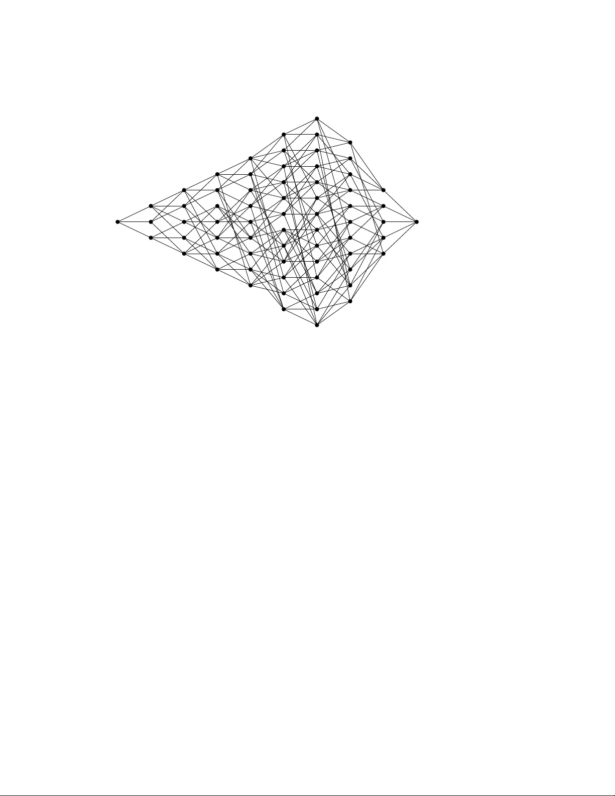
CS S COD ES FR OM THE BR UHA T O RDER O F COXETER GR OUPS KAMIL BRÁD LER Abstract. I introd uce a method to gen erate f amilies o f C SS codes with interesting code parameters. The object of study is Coxeter groups, both ﬁnite and inﬁnite (reducib le or not), and a geometrically moti vated partial order of Coxeter group elements named after Bruhat. The Bruhat order is kno wn to provide a link to algebraic topology – it doubles as a face poset capturing the inclusi on relations of the p -dimensional cells o f a regul ar CW co mplex and that is what ma kes it interesting f or Q EC code design. Assisted by the Bruhat face po set interval structure uniqu e t o Coxeter groups I show that the corresponding chain compl exes can be turned into multitudes o f CSS codes. Depending on the a pproach, I obtain CSS codes ( and their families) with controll ed stabilizer weights, for example [ 6006, 924, {≤ 14, ≤ 7 } ] (stabilizer weights 14 and 9) and [ 22880, 3432, {≤ 8, ≤ 16 } ] (weights 16 and 10), and CS S codes with highly irregul ar stabilizer weight distributi ons such as [ 571, 199, { 5, 5 } ] . F or the latter , I develop a weight-red uctio n method to deal with rare heavy st abilizers. Finally , I s how how to extract fo ur-term ( length three) chain complexes that can be interpreted a s CSS codes with a metacheck. 1. Intr od ucti o n Search and study of n ew quantum error-correcti on ( QEC) codes has been a signiﬁcant part of quantum computing theory research since its early days. Stabilizer codes [ 1 ] as a quantum equiva- lent of cl assi cal linear codes are the main object o f interest together with an import ant subcl ass of CS S codes [ 2 , 3 ], which is a t ype of QEC codes I focus here too. The discov ery of new codes is of a great theoretical interest but no wadays the main m otivator is the quest for a utilit y-scale univ er- sal f ault-tolerant quantum computer pursued (m ostly) by private sector . Physi cal and technol ogical constraints of the prospectiv e quantum computing pl atforms dictate the desired properties o f the used codes and their families. There is a very long list o f the code properties that n eeds to be eva lu- ated from the scala bilit y point of vi ew with regard to a giv en pl atform bef ore a decision is taken to implement it in the qu antum hardware and software. If the main ﬁgure of merit is just an asymp- totica lly constant encoding rate and linearly sca ling distance while the stabilizer w eight is bo unded then the answer points to good quantum LD PC ( low-density parit y check) codes who se ( existential) disco very is one o f the most important advances in recent quantum computing [ 4 – 8 , 15 ]. Whether they turn out to be practically usab le code f amilies in a ﬁnite regime is so far an open questio n. While waiting for the answer , researchers came up with constructiv e f amilies [ 9 , 10 ] o f ‘prett y good’ ﬁnite-size LDPC codes (su ch as codes with a constant or sl owly decrea sing rate and suboptimal but guaranteed dist ance scaling) with solid distances, decently bounded st abilizer weights [ 11 – 19 ] and with a gro wing focus on the scalabilit y of performing logi cal operations in a fault-tolerant manner . In this regard they already started to outperform the surface code [ 20 – 22 ] – the gold st andard of QEC codes one might ca ll a ‘not-so-bad’ LD PC code. Ev en for current best prett y good LDPC codes it remains to be seen how practically usef ul they are on a very l arge scale. As already mentioned, the distance and rate scaling is not the only per- forman ce indicator to watch from the scalabilit y point of view . There is a considera ble interest to 2 CSS COD ES FROM TH E BR UHA T ORD ER O F CO XET ER GRO UP S come up with new code creatio n methods even at the cost of the code f amilies not necessarily be- ing LDPC [ 23 – 27 ]. My proposal, which is ba sed on the properties o f Coxeter groups, falls into this category . Coxeter groups are a family o f discrete groups. They ﬁgure promin ently in vario us areas o f mathematics but their origin is geometrical as a formalizatio n of a ( ﬁnite) group of reﬂectio ns in Euclidean geometry [ 28 – 30 ]. All ﬁnite irreducib le Coxeter groups were classiﬁed and they were f urther generalized to aﬃne Euclidean spaces as well as hyperbolic spaces of variou s signatures. The reﬂecti on hyperpl anes ( a s abstracted mirrors) can be shifted awa y from the origin in aﬃne v ector spaces, giving rise to tessell ations. Consequently , C oxeter groups for aﬃne reﬂection systems ( and hyperbolic a s well) are inﬁnite. Coxeter groups pro vide vario us mechanisms to generate C SS codes. Compactiﬁed aﬃne Eu- clidean spaces E d giv e rise to the d -dimensional toric codes [ 22 , 31 ] and their t wisted variants. Their asymptotic properties pale in comparison with the variet y and properties of the C SS codes one can get from tesselated hyperbolic spaces [ 32 , 33 ]. A diﬀerent constructio n is 2D and 3D color codes [ 34 , 35 ], which are again CS S codes that can be derived from regular ( or less regular) tessell a- tio ns. Color codes were originally introd uced witho ut ref erring to Coxeter groups b ut this philo sophy , adopted by many authors [ 31 , 36 , 37 ], is quite fruitf ul and leads to multiple genera li zations [ 38 ]. Finally , a recent work speciﬁca lly t argeting Coxeter groups introdu ced a diﬀerent C SS code con- structi on based on assigning stabilizers to the f acets o f polytopes constructed from Cayl ey graphs o f Coxeter groups [ 39 ]. This approach has a m ore combinatorial ﬂav or and is probably clo sest to the point of view adopted here of using combinatorial rather than geometrical properties of Coxeter groups. The constructi on introdu ced in this paper is yet another way of extracting CSS codes from Cox- eter groups. The structure of C oxeter groups admits sev eral diﬀerent partial orders and o ne of them is called the Bruhat order . It st ands out thanks to its rich properties encompassing combinatorics, geometry and algebrai c topology . In particular , every Bruhat poset ( partially ordered set) can be interpreted as a cell complex kno wn as a regular CW complex. More precisely , the partial order relation o f the Bruhat poset is in f act a face poset of closed cells of a cert ain manifold ordered by inclusi on. The manifold is a cellul ated d -dimensional sphere S d that comes with a remarkabl e in- ternal structure. The key discov ery [ 40 ] is the internal poset structure for the intervals of length t wo, three and four of any Coxeter group 1 – just what is necessary to decompose an arbitrary C SS code. I exploit it to generate C SS codes which are encoding qubits with high rates and respectab le distances. The internal structure ni ckn amed diamo nd- ( S 0 ), k -crown ( S 1 ) and S 2 -sphere decompo- sitio n is then an eﬃcient indicator where to apply a transformati on I call splicing. This operation, despite being quite a primitiv e st abilizer transf ormation, manages to prod uce interesting CSS codes from wildly diﬀerent Coxeter groups – both ﬁnite and inﬁnite – at the cost of uneven and sometimes heavy stabilizer checks 2 . I t ake the ﬁrst steps to t ame it by introducing a st abilizer w eight-redu ctio n method [ 42 ], which as a side result can be applied to an arbitrary CSS code. The ﬁnal result is a proced ure that I ca ll chain complex folding which allo ws to conv ert l onger Bruhat po sets into length t wo and three chain complexes. The former are again CS S codes but this time with a better st abilizer weight control. The latter are CS S codes equipped with a single met acheck. Almo st all codes are conjectured to be part of large ﬁnite or inﬁnite f amilies o f codes by closely foll owing the growth o f the underlying Coxeter groups. All C SS codes sho wed as examples hav e their distance probabilistica lly upper-bounded by Qdis- tRnd [ 43 , 44 ], whi ch is implemented as a GAP [ 45 ] library . Small er or lo w-distance codes are then 1 Length four intervals were classiﬁed just for ﬁnite W eyl groups [ 41 ] but rather than the cl assiﬁ cation itself it is mainly its existence that is used here. 2 I believ e that the uniqu e ‘microscopic’ insight into the code stru cture pro vided by the sphere decompo sition could be exploited more eﬃci ently by , for example, more advanced stabilizer transformati on methods. CSS COD ES FROM TH E BR UHAT ORD ER O F CO XET ER GRO UP S 3 exactly calculated by dist-m4i 3 also developed by L. Pryad ko and collaborators and conﬁrmed by another exact method used by Qubitserf 4 devel oped by S , . C ercelescu. I used both exact methods except for edge cases where either I lack time or memory . Ev erything else remains upper-bounded ( Qubitserf has a multithread option b ut it declares segmentation fault for larger codes – the tool is under dev elopment). Despite the diﬀ erences in the underlying algorithms the proba bilistic on es o f- ten a gree with the deterministic ones and that gives me more conﬁdence that they are accurate even for large codeb lock examples. In those cases I w ent to great lengths to corroborate the results by repeated sampling as well a s by deriving ( by yet another method) the actual logical P auli operators and ﬁnding the one(s) with the smallest weight. This obvious ly does not pro vide a prova ble lo wer bound but it serves as a sanit y check and ultimately increases the conﬁdence in the actu al estimates. That being said, some of the discov ered codes are very l arge and none of the distance-estimatio n methods allo ws me to claim that the chances of low ering the reported distance valu es are bey ond reaso n ab le doubt. In fact, I w ould be ab le to generate m uch larger codes based on Bruhat order but the computatio nal cost to get even a reasonab ly conﬁdent upper bound by [ 43 ] is just too high. This is the ﬁrst cav eat of the paper . The second one is the det ailed performan ce and iterative ( a symptotic and ﬁnite) behavi or of the introdu ced weight reducti on procedure. The S 1 ( 2 ) Bruhat- based codes are quite often high-rate/high-weight and the weight-red uctio n method is capa ble of red ucing the rate k / n by repeated ly increasing the physica l qubit number while the hope (but not the proof ) based on numerica l simulatio ns is that the distance is no n-decreasing. If true it is an econ omic wa y o f decreasing weight and keeping the codes’ good parameters. So there is a reaso n for optimism but its conﬁrmatio n is a major project on its own and therefore deferred for future inv estigations. The paper consists of the follo wing main parts: Section 2 introdu ces the principal method and its variants to obtain non-trivial C SS codes with interesting parameters described as CW chain com- plexes of length three and four . The former is a C SS code while the l atter is a CS S code equipped with a metacheck. S ectio n 3 introdu ces a weight-red uctio n method to deal with a negati ve byprod uct o f the code creation procedure, where some checks become too heavy . The paper lea v es plent y of open questio ns summarized in Conclusi ons, Section 4 , follo wed by Section 5 in the form o f severa l Appendices, where I collected useful facts about hom ology and chain complexes with perhaps less frequented but terminology-hea vy topics such as posets and regular CW complexes. This is for the sake of completeness even though the language of algebrai c topology is now a st andard tool in QEC research, having been used explicitly at least since the work of Freedman and Meyer [ 46 ] (implicitly , o f course, a lready in [ 20 ] posted years earli er), see also [ 47 ]. 2. C SS co d e co nstr ucti on Ev ery C SS code discov ered in this paper starts its life as an open interval ( w b , w t ) of a Coxeter system ( W , S ) , which is a graded f ace poset F ( S d ) capturing the inclusion relation of the p -cells of a regular CW decompositio n of a d -dimensi onal sphere S d , see Appendices in Section 5 for more detail. The f ace poset F ( S d ) is a C W ( d + 2 ) -chain complex and for a suﬃ ciently big d it giv es rise to shorter chain complexes o f interest. These structures are at the core o f the methods presented here so let’s f ormalize it. Deﬁnitio n 1. L et ( W , S ) be any Coxeter system and B = ( w b , w t ) be an open interv al o f the Bruhat order for w b , w t ∈ W . Thanks to Theorem 7 , B = F ( S d ) , where ℓ ( B ) = d + 2 is the length of B . I denote ( W , w b , w t , p ) 2 k + 1 to be a subpo set of F ( S d ) in the form of 2 k + 1 layers { l p } ∈ F ( S d ) of length p for − k ≤ p ≤ k whenev er ℓ ( w b ) ≤ p − k and p + k ≤ ℓ ( w t ) . 3 dist-m4ri 4 Qubitserf 4 CSS COD ES FROM TH E BR UHA T ORD ER O F CO XET ER GRO UP S Ev ery ( W , w b , w t , p ) 2 k + 1 is a face subpo set o f length 2 k + 1 − 1 = 2 k consisting of 2 k + 1 layers { l i } , p − k ≤ i ≤ p + k . For k = 1 its Hasse diagram is called a quantum T anner graph because it is a CSS code even though a trivial one – encoding zero logica l qubits (see Theorem 3 ). I will use the language of T anner graphs and f ace po sets interchangea bly but I will also need to use the chain complex terminology . Here it might get a little bit conf using because ( W , w b , w t , p ) 2 k + 1 is formally not a chain complex. Why? Finite chain complexes hav e t wo distinguished zero mod ules as their initial and termin al mod ules. If I co nsider an entire f ace poset F ( S d ) the zero mod ules are naturally present in the form of w b and w t . If , on the other hand, a f ace sub poset ( W , w b , w t , p ) 2 k + 1 o f length 2 k is extracted from F ( S d ) it is forma lly necessary to add comm on bottom and top elements that I will denote ˆ b and ˆ t in order to promote it to a chain complex of length not 2 k b ut rather 2 k + 2 , that is, consisting of 2 k + 1 + 2 = 2 k + 3 layers. This chain complex will be denoted ( W , w b , w t , p , ˆ b , ˆ t ) 2 k + 1 when ˆ b , ˆ t play an important role but otherwise I ab use notation and also call ( W , w b , w t , p ) 2 k + 1 a chain complex. The practical diﬀerence when describing how to obtain non-trivia l CS S codes later in the text ( codes having non-zero number of logi cal qubits) is null. An added advantage of introd ucing ˆ b , ˆ t is that [ ˆ b , ˆ t ] = ( W , w b , w t , p , ˆ b , ˆ t ) 2 k + 1 is call ed a closed poset interval (Sectio n C ) and ( ˆ b , ˆ t ) = ( W , w b , w t , p ) 2 k + 1 is an a ssociated open poset interva l. S o ev en though the n umber of l ayers between [ ˆ b , ˆ t ] and ( ˆ b , ˆ t ) diﬀers, the interval length of the posets is equal, that is ℓ ([ ˆ b , ˆ t ]) = ℓ (( ˆ b , ˆ t )) = 2 k + 2 . Longer chain complexes ( W , w b , w t , p , ˆ b , ˆ t ) 2 k + 1 ( or ( W , w b , w t , p ) 2 k + 1 ) for k = 2, 3 will be used as well as an intermediary step to again get T anner gra phs of non-tri vi al CS S codes. The main constru ction in this paper is ba se on a specia l propert y o f the Bruhat poset of Coxeter groups which is, in general, not shared by other discrete groups: They can be decompo sed into elementary spheres 5 , namely S 0 , S 1 and S 2 . Before discussing the code-making strategies it seems rea sonabl e to ﬁrst show a few examples o f Coxeter groups and their Bruhat order posets to get a hand le on the poset terminology and what is going o n here. I chose three examples that do not provide interesting codes due to their siz e b ut to me the evidence suggests that they are a part o f diﬀerent ( inﬁnite) code families and I will sho w that their bigger sib lings do provide interesting codes. Example. Coxeter system ( A 3 , { s 1 , s 2 , s 3 } ) : An inﬁnite class of Coxeter groups called A n is better kno wn as the symmetric groups S n + 1 o f order ( n + 1 ) ! . A n is one of the m ost import ant cl asses o f discrete groups whose vari ous properties and links to diverse areas o f mathematics hav e been inv estigated in detail. The Coxeter matrix for n = 3 is in Eq. ( 43 ) and the Bruhat poset is depicted in Fig. 1 . This is the only example where I will illustrate in det ail the rich poset terminology introdu ced in Appendix C f ollow ed by severa l sphere decompo sitions in Secti on F . The Bruhat order on A 3 is sho wn in the f orm of an undirected Hasse di a gram in Fig. 1 . The v ertices o f the graph are the group elements and the undirected edges are the co vering rel atio ns. The lo west ( bottom) element w b = id is on the f ar left and top el ement w t = s 1 s 2 s 3 s 1 s 2 s 1 is the rightmost vertex ( using the toppled con venti on). Hence the depicted poset is a closed interv al [ w b , w t ] . The poset is graded by the red uced word length f unctio n ℓ , where ℓ ( id ) = 0 and ℓ ( w t ) = 6 a lready in its red uced form and so ℓ ([ w b , w t ]) = 6 . Since | A 3 | = 24 the entire poset can de drawn but if necessary n othing prevents me from choosing a diﬀerent pair w b , w t to get a subpo set as lo ng as w b < w t holds. The poset’s H asse diagram is stratiﬁ ed by (v ertical) layers l i o f all incomparab le poset elements of rank i . So, for example, the number o f layer elements for i = 3 is | l 3 | = 6 highlighted as a purpl e line. In the CW interpret atio n of this poset, the open interva l ( id, s 1 s 2 s 3 s 1 s 2 s 1 ) is a regular CW decompo- sitio n of the S 4 sphere, where each l ayer l p , 1 ≤ p ≤ 5 , is occupied by | l p | ( p − 1 ) -cells ( ( p − 1 ) -f aces), 5 S d sphere decompositi ons for d > 2 are possib le but they can’t be called elementary and mainly they do not seem to be kno wn through classiﬁcatio n. CSS COD ES FROM TH E BR UHAT ORD ER O F CO XET ER GRO UP S 5 w b = id w t = s 1 s 2 s 3 s 1 s 2 s 1 l 0 l 1 l 2 l 3 l 4 l 5 l 6 Fi gure 1. The Bruhat order of the W eyl group A 3 , Eq. ( 42 ). The open interva l ( w b , w t ) is a face poset of a regular CW -cellul ated sphere S d for d = 4 . The vertices can be seen a s ( p − 1 ) -cells ( 1 ≤ p ≤ d + 1 = 5 ) ordered by in clusion or a s Coxeter group elements w = s i 1 . . . s i p ∈ A 3 o f the redu ced length ℓ ( w ) = p related by a reﬂecti on. The edges are cov ering relations o f the Bruhat order . see S ectio n D and F . The cov ering rel atio n becomes a closed cell inclusio n and the poset therefore becomes a face poset F ( S 4 ) . Ev ery triple of l ayers { l i } i = p − 1, p , p + 1 is a T anner graph of a CS S code for all 2 ≤ p ≤ 4 , where the l ayer l p is assigned to dat a qubits and l p ± 1 are X and Z stabilizers or vice versa. This avo ids the left- and rightm ost triple ( p = 1 and p = 5 , respecti vely) which, despite being legitimate C SS codes, are not practically as interesting as the rest due to the presence of a single vertex (stabilizer). The triples { l i } I just described are examples of ( W , w b , w t , p ) 3 from Deﬁnition 1 as the building b locks o f non-trivial C SS codes introdu ced l ater . The Hasse diagram of the Bruhat poset of a Coxeter group often has a geometrical interpret atio n. Although nowhere in this w ork I use any such constructi on it is w orth mentioning it in the case of A 3 . By comparing the left or right Cayley graphs based on the generating set consisting of the simple reﬂecti ons s i (see S ectio n A ) with the additional genera l reﬂectio ns t j responsib le for the Bruhat po set co vering rel atio ns (see Eq. ( 45 )) it foll ows that the Bruhat order uses Cayley graphs as a scaﬀold for any C oxeter group. So, given a C oxeter group’s Cayl ey graph with the corresponding weak order (see Section A ) the Bruhat order on the same group is obt ained by adding some m ore edges to the corresponding Cayley Hasse diagram. The left (right) Ca yley gra ph o f A n tessellates R n . F or n = 3 it is called a perm ut ahedron or a truncated octahedron and it made appearan ce in several QEC code constru ctions [ 38 , 48 ]. I depict how the ‘Bruhat boo sted’ perm ut ahedro n looks like in Fig. 2 , where one can see additional edges inside the perm utahedron and also inside the hexago n al f aces – all coming from the non-simpl e reﬂectio ns. Similar enhancements are possib le for other C oxeter groups whose Cayley graphs have a geometrical interpret ation (such as aﬃne and hyperbolic tessell atio ns). Let’s turn the attentio n to exemplif ying the sphere decompo sitio n – a feature uniqu e to Coxeter groups as far as the author is aware. The spheres mo st relevant to any 3-l ayer poset representing a trivial CS S code are S 0 , S 1 and S 2 , see Fig. 14 . Let’s choose a speciﬁc triple { l i } i = 2,3,4 in Fig. 1 ( hence p = 3 ). The S 0 sphere who se poset is nicknamed the di am ond poset can be easily identiﬁed by choosing any pair of verti ces from layers l 2 and l 4 o f every ( A 3 , id, s 1 s 2 s 3 s 1 s 2 s 1 , 3 ) 3 and checking whether they share zero or t w o verti ces from l 3 . No other option is possib le [ 40 ], see Theorem 8 (1). 6 CSS COD ES FROM TH E BR UHA T ORD ER O F CO XET ER GRO UP S Fi gure 2. The Bruhat poset of A 3 from Fig. 1 in a geometri cally friend ly wa y as a truncated oct ahedro n ( also kno wn as a permutahedron in combinatorics) with some additi onal inner-face edges whose origin are non-simple reﬂectio ns. The orange balls are the b l ack vertices and the rods connecting them are the cov ering relations. A m ore interesting case for this work is the S 1 decompositi on in terms of the k -cro wn poset. The k -crown posets are length three posets and so to identif y a k -crown in l ayers { l i } , i ∈ { p − 1, p , p + 1 } one has to look for the corresponding bottom element ˆ b in layer l p − 2 or for the top element ˆ t in l ayer l p + 2 . One then obt ains a left or a right k -crown poset. This decompositi on is the main tool to get no n-trivial CS S codes and Sectio n 2.2.1 contains a det ailed descripti on. Finally , for the S 2 decompositi on, that is, a poset of length four , one looks for the bottom/top element ˆ b / ˆ t in layers l p ∓ 2 . I highlighted t wo o f the identiﬁed S 2 face posets in Fig. 3 together with the corresponding CW complexes in Fig. 4 . A complete cl assiﬁ cation of the S 2 CW complexes for 4 3 5 2 1 5 2 6 4 3 1 2 4 3 5 1 4 3 5 2 1 5 2 6 4 3 1 2 4 3 5 1 Fi gure 3. The T anner graphs of the ( A 3 , id, s 1 s 2 s 3 s 1 s 2 s 1 , 3 ) 3 CS S code ( consisting o f layers l 2 , l 3 and l 4 in Fig. 1 ) with diﬀerent highlighted S 2 posets in magenta. The connected bottom and top elements ˆ b and ˆ t from neighboring l ayers are not depicted. The correspo nding C W compl exes are depicted in Fig. 4 . CSS COD ES FROM TH E BR UHAT ORD ER O F CO XET ER GRO UP S 7 4 3 5 2 4 6 5 3 4 2 1 2 3 4 1 4 3 6 2 5 4 5 1 2 Fi gure 4. S 2 regular CW complexes corresponding to the ma gent a sub posets in Fig. 3 with the same color coding and numbering: red vertices (say X checks), b lack edges (dat a qubits) and blues faces ( Z checks) including the ambient on es. The CW compl ex o n the left is recognizab le as a tetrahedron. Also cf. the classiﬁ ed S 2 CW complexes n umber 1 and 3 in Fig. 15 . w b = id w t = s 1 s 2 s 3 s 4 Fi gure 5. The Bruhat/wea k order of the red ucib le Coxeter group C × 4 2 . The open interva l ( w b , w t ) o f length fo ur is a f ace poset F ( S 2 ) . ﬁnite W eyl groups comes from [ 41 ] and is listed in Fig. 15 . I discuss in Sectio n 2.2.2 how to use the S 2 to a gain create non-trivia l C SS codes. Example. R educib le group C × n 2 : The cyclic group C 2 is a t w o-element Coxeter group with a simple structure ( ( A 1 , { s 1 } ) in C oxeter’s classiﬁ cation). Its Ca yley graph is an edge and technica lly it is also a Bruhat f ace poset although it is an empt y poset without any cells (faces). To get a non-trivial poset one t akes C 2 × C 2 whose poset is the S 0 face poset: the diamond graph. It is formed by the Cartesian prod uct (the same graph product used in the co nstructi on o f the hypergraph product codes [ 12 ]) of t wo edges resulting in a square and this is a lso the C 2 × C 2 Bruhat poset. S o the Ca yley and Bruhat orders coincide and this holds for all n . What makes this group family potentially interesting is its relative simplicit y , where the Ca yley/Bruhat poset o f C × n 2 is an n -dimensiona l cube a lso kno wn as a Boolean l attice ( a specia l kind o f poset [ 49 ]), together with the fact that it leads to interesting codes as I will show in Section 2.2.4 . Ca se n = 4 is depicted in Fig. 5 . Example. As the ﬁnal example I t ake an inﬁnite-dimensional Coxeter group, namely one from an inﬁnite family of the so-called hyperboli c triangle groups [ 28 ]: ( ∆ α , β , γ , S ) = 〈 s 1 , s 2 , s 3 | ( s 1 s 2 ) α , ( s 1 s 3 ) β , ( s 2 s 3 ) γ 〉 , (1) such that 1 /α + 1 /β + 1 /γ < 1 . They ﬁgure promin ently in the QEC code design a s codes created by compactif ying hyperbolic tessellations. Let the triangle group be α = 2, β = 3, γ = 7 . I choose the standard w b = id and w t = ( s 1 s 2 s 3 ) m in its red uced f orm. It is a loca lly ﬁnite group and so I can 8 CSS COD ES FROM TH E BR UHA T ORD ER O F CO XET ER GRO UP S w b = id w t = ( s 1 s 2 s 3 ) 3 Fi gure 6. A subpo set of the Bruhat order of the triangle hyperbolic group, Eq. ( 1 ), for α = 2, β = 3, γ = 7 . The open interva l ( w b , w t ) is a face poset F ( S 8 ) . a gain depict its ranked Bruhat poset in the form o f a Hasse diagram. Choosing m = 3 the poset is depicted in Fig. 6 . and unlike the previous t wo examples it is asymmetric. That is a t ypical poset Hasse diagram one gets fro m a randomly cho sen C oxeter group unlike the highly symmetric groups A n or C × n 2 sho wn previous ly . 2.1. Trivia l co d es As a warm-up, the structure of the length two intervals in Theorem 8 (1) in terms of the S 0 spheres and the corresponding di amo nd posets will be used a s an alternativ e proo f o f the st atement that every three-l ayer poset is a valid CS S code. I assign a layer l p o f p -cells to dat a qubits and the l ayers of ( p ± 1 ) -cells to X and Z checks ( or vice versa) for any consecutiv e triple of layers { l i } , i ∈ { p − 1, p , p + 1 } in the interval [ w b , w t ] . More forma lly: Lemma 1. L et ( W , w b , w t , p ) 3 be a length t w o chain complex such that and ℓ ([ w b , w t ]) ≥ 5 . Further , let Q ⊆ l p be a poset l ayer o f rank p . Whenever X ⊆ l p − 1 and Z ⊆ l p + 1 are such that for all x ∈ X and z ∈ Z , either ( x , z ) ⊆ Q or ( x , z ) ∩ Q = ; then the operators { Y q ∈ Q : x ⋖ q X q : x ∈ X } and { Y q ∈ Q : q ⋖ z Z q : z ∈ Z } deﬁne a CS S code where any X and Z check ov erlap on either z ero or t wo qubits. Proo f . L et x ∈ X and z ∈ Z correspond to X and Z checks that both act on some qubit q ∈ Q . Then by assumpti on, ( x , z ) ⊆ Q , x < z and ℓ ( z ) − ℓ ( x ) = 2 . Therefore ( x , z ) contains t w o elements by [ 40 ] ( it is reprod uced in Propositi on 8 (1)), where [ x , z ] wa s dub bed the diamond poset in Appendix F . ■ CSS COD ES FROM TH E BR UHAT ORD ER O F CO XET ER GRO UP S 9 Note that the codes o f Theorem 1 can encode logica l qubits b ut their discov ery relies on an in- tractabl e process of systematically generating subsets X or Z and checking the code properties. It is equival ent to a systematic rem ova l of the row s of the corresponding PCMs. The diamo nd ( S 0 ) decompositi on of any ( W , w b , w t , p ) 3 CS S code sketched in Sectio n 2.2.2 makes it signiﬁcantly more tractabl e b ut co mpared to the main decompo sition method the resulting non-tri vi al codes are much less interesting and therefore not worth o f pursuing. The starting point o f more eﬃci ent code constructi ons will be a special case o f the previous lemma when Q = l p and X = l p ± 1 , Z = l p ∓ 1 , where ( W , w b , w t , p ) 3 uniqu ely determines a CSS code. It turns out, how ever , that every such code is trivial and the reason is that the underlying manifold, a d - dimensio n al sphere corresponding to the interva l ( w b , w t ) , where ℓ (( w b , w t )) = d + 2 , supports zero logica l qubits for any d , W , p thanks to the kn own properties of the S d hom ology groups: H 0 ( S d , Z 2 ) = H d ( S d , Z 2 ) = Z 2 , (2a) H i ( S d , Z 2 ) = 0 otherwise . (2b) This perhaps intuitiv e fact is s hown in the f ollo wing lemma using the termin ology of Section D.1 : Lemma 2. L et ( W , w b , w t , p , ˆ b , ˆ t ) 3 be a length t wo chain compl ex and X a regular CW compl ex obtained by grad u ally remo ving the consecutiv e l ayers fro m its f ace poset F ( S d ) . Then H p ( X , Z 2 ) = 0 . Proo f . All open intervals ( w b , w t ) o f length d + 2 pert aining to the Bruhat order of a Coxeter group are graded f ace posets F ( S d ) of a regul ar C W complex homeom orphic to S d [ 40 ]. As such, the CW complex’s Betti numbers are β 0 = β d = 1 and zero otherwise, see ( 2 ) and Section D.1 . The boundary of the ( d + 1 ) -dimensio n al v oid are all d -dimensi onal cells. I remo ve from the f ace poset the layer ranked as r = d corresponding to these d -cells and add a common top element ˆ t to be ab le to properly deﬁne all homol ogy groups and the corresponding Betti numbers. In this way I obt ain a new C W complex X ′ whose dimensio n is redu ced by one compared to the original sphere S d . The new complex is not, in genera l, homeom orphic to a sphere since by remo ving all the d -cells I eﬀectiv ely introduced a number o f d -dimensio n al v oids that are counted by the highest Betti number o f X ′ . Hence I reduced the ( d + 1 ) -tuple o f Betti numbers β ( S d ) to a n ew d -tuple β ( X ′ ) : β ( S d ) = ( 1, 0, . . . , 0, 1 ) → β ( X ′ ) = ( 1, 0, . . . , 0, β d − 1 ( X ′ )) , (3) where β d − 1 ( X ′ ) = rank ker ∂ d − 1 as foll ows from ( 55 ). The rest of the Betti numbers remains the same since I ha ven’t touched the other boundary operators. I contin ue by remo ving layer by l ayer , thus era sing the previou sly introdu ced vo ids and introdu cing the v oids of one dimension less, again counted by the corresponding Betti n umber . In the penultimate step where only three layers of the Hasse di agram depicting the f ace poset are left I red uced S d to a manifold X ′′ whose Betti numbers are β ( X ′′ ) = ( 1, 0, β 2 ( X ′′ )) . (4) corresponding to the chain complex ˆ t → C 2 → C 1 → C 0 → ˆ w b . (5) I now generalize this process to any neighboring triple of layers. Let the desired triple of layers from F ( S d ) , without loss of generalit y , be l i , i ∈ { p − 1, p , p + 1 } . F ollo wing the same procedure described in the previo us paragra ph I stop upon reaching a CW complex that I now call X ′ , whose Betti ( q + 1 ) -tuple reads β ( X ′ ) = ( 1, 0, . . . , 0, β q ( X ′ )) (6) for q ≤ d . I n ow reinterpret the face poset of X ′ by considering its q -cells to beco me the ( d − q ) -cells o f e X ′ . Indeed, there is a complete freedom from which end ( bottom w b or top w t ) of F ( S d ) I start assigning 0-cells. I eﬀecti v ely dualized X ′ and with this transformati on in hand I may again st art 10 CSS COD ES FROM TH E BR UHA T ORD ER O F CO XET ER GRO UP S rem o ving the highest cells, l ayer by l ayer , b ut this time from e X ′ (that is, from the other side of the Hasse dia gram of the origin al X ′ ). In the penultimate step I arrive at β ( e X ′ ) = ( β p − 1 ( e X ′ ) , 0, β p + 1 ( e X ′ )) , (7) where β p + 1 ( e X ′ ) ≡ β q ( X ′ ) from Eq. ( 6 ). Graphi cally , I obt ained the chain complex ˆ t → C p + 1 → C p → C p − 1 → ˆ b , (8) which I can identif y with ( W , w b , w t , p , ˆ b , ˆ t ) 3 from Deﬁnition 1 . Since β p ( e X ′ ) = 0 the claim follo ws. ■ Corollary 3. The cl osed interval [ ˆ b , ˆ t ] = ( W , w b , w t , p , ˆ b , ˆ t ) 3 ( chain complex o f length t wo) corres ponds to the open poset interval ( W , w b , w t , p ) 3 with three layer ( see Deﬁnition 1 ) that can be interpreted as a T anner graph of a CSS code. Thanks to the p -th homology group being zero it encodes z ero logical qubits. This result ba sically sho ws that ‘slicing’ a trivial manifold along any triple o f consecutiv e layers of its CW f ace poset still yields a topologica lly trivial structure. This looks like a showstopper for the purpose of generating interesting QEC codes. Indeed, the trivial ( W , w b , w t , p ) 3 CS S codes are by constru ction topologica l since all verti ces o f the resulting T anner graph were identiﬁed with closed cells of a cert ain dimension. One directi on could be to seek quotient maps just like it was don e for the spaces o f constant curvature. But this has led to a large variety o f codes only in the case of hyperbolic spaces [ 32 , 33 , 50 ], whereas for the spherical and planar geometry it ‘merely’ pro vides codes on the projectiv e plane RP n (such as the [ 9, 1, 3 ] Shor code for n = 2 ) and the generalized toric codes. Giv en the proximit y of the ( W , w b , w t , p ) 3 codes to the spherical geometry this strategy does not look promising. Instead, let’s use the particular structure o f the high-dimensio n al s pheres obtained from the Bruhat order on Coxeter groups. This structure is giv en by the sphere decompositi on of the length t w o, three and four intervals described in Appendix F . 2.2. No n-trivia l co d es My ﬁrst strategy to m odif y a ( W , w b , w t , p ) 3 CS S code to encode logica l qubits will be with the help of Theorem 8 and one of the three w ay s ev ery 3-l ayer poset ( a C W chain complex o f length t wo or a T anner graph) giv en by the Bruhat order can be decomposed into elementary building b locks by: (1) the diam ond posets, (2) k -crown posets and, (3), the posets f or Hultman’s 24 S 2 spheres [ 41 ], see Fig. 15 , if the used Coxeter group is of a W eyl t ype. If it is not a W eyl group, it is still not an issue since any new sphere can be easily identiﬁed and added to the list, see S ectio n F for more detail. When I sa y easily , it will be clear that once a face poset of ( W , w b , w t , p ) 2 k + 1 is deriv ed ( alw ays n eeded in the follo wing analysis) there is no computatio n al complexit y hiding in ﬁnding the corresponding S 0 , S 1 or S 2 sphere decompositi ons. It is less clear , how ever , what the complexit y is to actually get the ( 2 k + 1 ) -l evel poset or ev en the entire initi al poset F ( S d ) for an interv al [ w b , w t ] , C oxeter group and its order . Indeed, this probl em goes deep and amo ng other things it touches the complexit y o f the rewrite rules necessary to ﬁnd the reduced length of a word for a general ﬁnitely presented inﬁnite discrete groups such as inﬁnite Coxeter groups. The kno wn results are encoura ging [ 51 ] but this is a topic for a separate inv estigation. Ev en though the Coxeter groups studied here are small enough for us not to be bothered by these fundament al issues, they will provide quite large codes going bey ond what o ne wo uld call toy CSS code examples. 2.2.1. S 1 ( cr o wn) d e c o mpositi o n I ﬁrst deﬁne an operation I call ‘stabilizer splicing’. F or the notation see Section E . CSS COD ES FROM TH E BR UHAT ORD ER O F CO XET ER GRO UP S 11 splice Z Fi gure 7. (Left) A T anner graph of the [ 4, 2, 2 ] code with red undantly protected qubits to illustrate the n egative eﬀect of splicing. (Right) Z st abilizer (indicated in b lue) s plicing exposes the data qubits to X errors. Deﬁnitio n 2. Let H X , H Z be PCMs o f an arbitrary C SS code whose rows are denoted h i X , h j Z . A spliced X stabilizer ˜ H X is obt ained from H X by choosing I ⊆ [ dim H X ] to generate a new ( linearly- dependent) X st abilizer ˜ h k X = X i ∈ I h i X mod 2, (9) such that ˜ h k X substitutes h i X for all i ∈ I . Simil arly f or the spli ced Z st abilizer ˜ H Z . Spli ced stabilizers are va lid PCMs. That is, ˜ H X ˜ H T Z = 0 holds thanks to the linearit y of the splicing operatio n ( element-wise sum mod ulo t wo). This and related constru ctions will be the main tool in transforming trivial Bruhat-based CS S codes to no n-trivial ones. But what can be expected from the spli ced CSS codes? At ﬁrst sight it doesn’t look encoura ging. I present t wo of its n egative properties. First, there is no obvio us guarantee that the resulting CS S code is protecting all or ev en any logica l/physical qubit. Consider an ov erprotected [ 4, 2, 2 ] code with t wo X and t wo Z checks coupled to all four dat a qubits. Splicing the X or Z st abilizers will leav e the data qubits unprotected, see Fig. 7 . Second, the spli cing changes the st abilizers’ weights. Some qubit connecti ons (that is, the edges of a T anner graph) disa ppear and, in genera l, some o f the new spliced st abilizers become heavi er but in a highly non-unif orm way s hown later in Fig. 9 . Despite these issues splicing turns out to be quite usef ul in general and mainly in connecti on with the S 1 decompositi on of the ( W , w b , w t , p ) 3 codes. I will describe an algorithm whose main input is the complete k -crown structure of a chosen code ( W , w b , w t , p ) 3 . k -crowns are not unknown structures to QEC practition ers. Although it is a length three poset du e to the presence of the bottom and top vertices (see ˆ b , ˆ t in Fig. 14 for k = 7 ), once both are remo ved one is left with a classica l T anner graph of a (redundant) k -repetition code. Similarly , if either ˆ b or ˆ t is remo ved a quantum T anner graph of a (trivia l) quantum C SS code with redundant st abilizers of one t ype is obtained. Giv en a ( W , w b , w t , p ) 3 CS S code I will introduce the left and right k -crown graphs. T o this end, consider a lo nger chain complex ( W , w b , w t , p ) 5 consisting o f ﬁve consecutiv e layers l p − 2 , l p − 1 , l p , l p + 1 and l p + 2 o f the Bruhat f ace poset F ( S d ) for a suﬃci ently big d . Then according to Theorem 8 , item (2), f or each pair o f elements ˆ b ∈ l p − 2 , ˆ t ∈ l p + 1 there exists a k -cro wn poset with this bottom and top element. Such po set will be call ed a left k L -cro wn poset. Simil arly , for each pair of elements ˆ b ∈ l p − 1 , ˆ t ∈ l p + 2 there exists a k R -cro wn poset equipped with this bottom and top element. Any such S 1 sphere will be called a right k R -cro wn poset. I ﬁnd all left and right k L / R -cro wns by iterating o ver | l p − 1 | × | l p + 2 | + | l p − 2 | × | l p + 1 | possibilities and co nsider their sub posets obt ained by remo ving w b from all left k L -cro wns and w t from all k R -right crowns. The collectio n of these subposets will be denoted { F L ( S 1 ) } and { F R ( S 1 ) } – Fig. 8 illustrates the constructi on. 12 CSS COD ES FROM TH E BR UHA T ORD ER O F CO XET ER GRO UP S F L ( S 1 ) F R ( S 1 ) l p − 2 l p − 1 l p l p + 1 l p + 2 ( W , w b , w t , p ) 3 Fi gure 8. Fiv e poset layers l i , p − 2 ≤ i ≤ p + 2 o f a general Bruhat poset F ( S d ) used to ﬁnd a ll left and right k L / R -cro wn posets of a CS S code ( W , w b , w t , p ) 3 . The left k L -cro wn is illustrated f or k L = 3 in cyan and the right k R -cro wn f or k R = 4 in ma genta. The terminal vertices ( ˆ b for the left crown and ˆ t f or the right crown) and their incident edges that do not participate in the C SS code are remo ved (indi cated by the red crosses). Algorithm 1 is a pseudocode describing the process of obtaining a non-trivia l C SS code from a ( W , w b , w t , p ) 3 CS S code. In words, I randomly choose a tot al number κ o f left or right k -crowns with probabilit y ℘ 6 . This is a bias introduced to t ake into account the asymmetric T anner graphs o f ( W , w b , w t , p ) 3 . A t ypica l Bruhat order-based code has a diﬀerent number of X or Z checks and an ev en splicing w ould lead to suboptima l codes. The bias parameter can be calculated in diﬀerent wa ys. I use ℘ = |{ F L ( S 1 ) }| |{ F L ( S 1 ) }| + |{ F R ( S 1 ) }| b ut another option could be ℘ = | l p − 1 | | l p − 1 | + | l p + 1 | , where | l p ± 1 | is the number of left/right check qubits. Another import ant parameter is the ov erlap λ . When a new k -crown is pi cked, the corresponding left/right checks can coincide with the previous ly chosen left/right checks in at most λ instances. This turns out to be quite an import ant parameter , where the best codes are found for λ = 1 . Some choices of κ , λ may not be ( or are unlikely to be) 6 The use of the left ( L ) and right ( R ) notation reﬂects the verti cal arrangement of the f ace posets/T anner graphs used in this paper . It then lets us decide whether L = X ( Z ) and R = Z ( X ) . CSS COD ES FROM TH E BR UHAT ORD ER O F CO XET ER GRO UP S 13 Algorithm 1 k -crown ( S 1 ) spli cing of a ( W , w b , w t , p ) 3 CS S code 1: Input : 2: PCMs H L , H R o f a ( W , w b , w t , p ) 3 CS S code. 3: All left and right k -crown sub posets { F L ( S 1 ) } , { F R ( S 1 ) } o f the ( W , w b , w t , p ) 3 CS S code. 4: T otal number κ of k -crowns to be spliced. 5: Overlap parameter λ , cut-o ﬀ parameter c and bias probabilit y ℘ . 6: O utput : 7: PCMs ˜ H L , ˜ H R o f the spli ced ( W , w b , w t , p ) 3 CS S code. 8: procedure Cr ownS plice ( H L , H R , { F L ( S 1 ) } , { F R ( S 1 ) } , κ , λ , ℘ , c ) 9: n ← 0, I ← ; , J ← ; 10: f or m ← 1 to κ do 11: repeat 12: Flip a biased coin o f probability ℘ to pick an el ement of { F L ( S 1 ) } or { F R ( S 1 ) } 13: Find the PCMs’ ro ws { h m L } or { h m R } to be s pliced 14: ( I m ← indrow [ { h m L } ] and J m ← ; ) or ( I m ← ; and J m ← indrow [ { h m R } ] ) 15: ▷ #The function indrow identiﬁes the ro w indices 16: n ← n + 1 17: until | I ∩ I m | ≤ λ or | J ∩ J m | ≤ λ or n > c 18: I ← ∪ m I m 19: J ← ∪ m J m 20: end for 21: proced ure S pli ce ( H L , H R , { I m } , { J m } ) 22: ˜ H L ← H L 23: ˜ H R ← H R 24: end procedure 25: end procedure satisﬁed and so a cut-o ﬀ parameter c is introd uced to av oid getting stuck in a loop. The sub proced ure Spli ce is the actual splicing a s described in Deﬁniti on 2 . Once ˜ H L , ˜ H R are obtained, the data qubits that became decoupled from one or both checks are rem o ved. This doesn’t spoil the comm ut atio n relations. The dist ance parameter d = min [ d L , d R ] is then estimated (upper-bo unded) and exactly veriﬁed by dist-m4ri 3 or Qubitserf 4 if time or mem ory permits. The choice of a tripl e of input parameters κ , λ , c has to be optimi zed but it is f airly ea sy to guess a critical κ valu e, where the number of logical qubits becomes non-zero. Note that one can observe that the st abilizers o f the ( W , w b , w t , p ) 3 codes are highly ov ercomplete, that is, dim H X / Z > rank H X / Z and from the diﬀerence it is straightforward to dedu ce an interesting κ regime. In fact, the behavi or of Algorithm 1 is such that the switch from trivial to n on-trivial codes is not a grad u al transitio n as a f unctio n of κ . S o there is no need to sweep large swaths of the parameter space. Algorithm 1 prod uces just a single code inst ance and as I mentioned previo usly there is no guarantee that the code is interesting. It is therefore repeated with the same input parameters but ev en the largest codes presented in the next sectio n were obtained without t aking an excessiv e number o f samples. The main factor preventing me from going to even larger trivial codes as a starting point is not the time complexit y of t aking many samples but rather the need to estimate the dist ance each time. All tools I use are either sampling a lgorithms themselv es [ 43 ] or their compl exit y scal es bad ly 3 , 4 ( a s a matter of inevitabilit y) and this prev ents from going f urther without using additi onal parall el comput atio n al reso urces. 14 CSS COD ES FROM TH E BR UHA T ORD ER O F CO XET ER GRO UP S I , nev ertheless, introd uce a random proxy method to crown splicing in S ectio n 2.2.3 . In this ca se, I completely disregard the code’s intern al structure and simply splice a random number o f random pairs of X or Z T anner graph verti ces ( could be genera li zed to random n -tuples). Despite t aking a small number of random samples the method is remarkab ly stabl e and provides almo st identical codes with high probabilit y . Ho w good are these codes? Random spli cing applied to ( W , w b , w t , p ) 3 CS S codes yields (m ost of the time) sub par codes to crown spli cing in terms of both the dist ance and mainly the st abilizer weight. But it is quite informati ve as what to expect should the crown splicing procedure be performed. Additionally , it points to an even more exciting possibilit y that the crown posets do indeed play a role in the internal structure of the Bruhat codes derived from Coxeter groups. I lea ve this a s a major open questi on. Before sho wing some of the fo und codes, I mentio n in passing that the sets { F L ( S 1 ) } and { F R ( S 1 ) } contains k -crowns f or vario us k ’s and they correspond to 2 k -cycles as depicted in Sectio n F . Amo ng them is the smallest one, k = 2 , and the corresponding 4-cycle. They exactly correspond to the girth of the T anner gra ph and serve as a measure of how certain decoding algorithms perf orm [ 52 ]. It is not clear if the short cycles can be entirely av oided by exploring or designing Coxeter groups. Moreo ver , the splicing procedures, in gen eral, alter the cycle structure o f the codes. 2.2.2. The c as e o f S 0 and S 2 d e co mpositi ons The cro wn decompositi on hit the sw eet spot when it comes to the derivati on of no n-trivial CS S codes. But as on e can see in S ectio n F , all k -crown graphs are made o f diamonds (the S 0 diamo nd posets) and all S 2 posets are made of k -crowns. Can they be used for non-trivia l code creatio n? Besides splicing, there exists another strategy to obtain non-trivia l codes suitabl e to the di amo nd structure. It is simply by the systematic remo val of ro ws from the X or Z st abilizer . Ho wev er , without any internal stru cture, this procedure is hopelessly in eﬃci ent due to the combinatorial explosio n in the number of possibilities o f the checks to remo ve. This is not the strategy I am going to pursue here b ut it is worth mentioning that the internal structure of the trivial codes in terms o f their di am ond posets is indeed usef ul. If I remo ve pairs of X , Z checks forming a diamo nd non-trivia l codes are obtained again and in a signiﬁcantly more eﬃci ent wa y than just randomly remo ving st abilizer rows. Indeed, once all the di am onds are tracked (there are at most | l p − 1 | × | l p + 1 | of them) they pro vide the desired pairs of checks. The upside is that the resulting C SS codes do not suﬀ er from the st abilizer weight gain like for k -cro wn splicing. The downside is that the code parameters such as the dist ance and mainly the rate are worse, see T ab le 1 . Ho w does the cro wn spli cing compare to the S 2 splicing? Again, using the length four chain complex like in the crown decompositio n I can ﬁnd all S 2 posets as classiﬁed in [ 41 ] for W eyl groups and depicted in Fig. 15 or ev en, in general, new ones for non- W eyl gro ups. With this input, a simple m odiﬁcati on of Algorithm 1 is used. Unlike the left and right k -crowns, where one of the check t ypes is alwa ys a single vertex (so nothing to splice), every S 2 poset contains m ore than one check o f both the X and Z type. They are then spliced ( each t ype separately). Ho wev er , as explained in Section F , k -crowns are the cycles visible in Fig. 15 depicting the C W complexes of S 2 spheres. One ma y guess that thanks to the ‘correlated’ X and Z splicing the S 2 cannot gen erate better codes than cro wn spli cing. Indeed, giv en a code obt ained from the S 2 splicing one can f ormally transform it into a code obtained from some crown spli cing but not vice versa. Therefore, crown splicing is a richer proced ure to get non-trivia l codes. Ho wev er , the k -crowns in a given C W S 2 complex share edges (t ypica lly more than on e) and this corresponds to greater cro wn o verlapping than I used in Algorithm 1 by choosing λ = 1 . So this t ype of splicing can pro vide new codes t ypica lly not fo und by crown splicing and I indeed did ﬁnd one example, see T ab le 1 . Another advantage of the S 2 splicing is the speed du e to a small er number of the S 2 posets compared to the left and right k -crowns. There is another , speculativ e, option: that the structure of the S 2 posets has something to CSS COD ES FROM TH E BR UHAT ORD ER O F CO XET ER GRO UP S 15 do with the existence of interesting codes and their splicing should be preferred. I lea v e it as another open questi on. 2.2.3. O ther CSS co d e co nstr ucti ons – rando m spli cin g and chain c omplex fo lding In Section 2.2.1 I sho wed ho w to decompose any ( W , w b , w t , p ) 3 CS S code in terms of the k -crown posets. The results obt ained by splicing based on this approach are quite interesting codes – at lea st when it comes to the number of encoded qubits and dist ance. The heuristic code discov ery adventure could end here but are there other ways of ho w to make the ( W , w b , w t , p ) 3 CS S codes non-trivia l ( and competitiv e in terms of the code parameters)? In this section I sacriﬁce the detailed structure o f these codes in f av or o f a more, one co uld say , blunt but at the same time m ore eﬃci ent approach o f how to get interesting codes. The introduced procedure is n ot o nly m ore comput atio n ally feasib le compared to crown splicing b ut also all o ws me to extend the scope of where the Bruhat order of Coxeter group can be applied. Namely , by employing the chain complexes of lengths greater than t wo I describe a method of ho w to obtain CS S codes with metachecks of one t ype, which were sho wn to be useful for single-shot decoding [ 50 , 53 – 56 ]. In terms o f chain complexes the S 1 or S 2 splicing procedure can be summari zed as C p + 1 H T Z → C p H X → C p − 1 splice 7− → ˜ C p + 1 ˜ H T Z → ˜ C p ˜ H X → ˜ C p − 1 . (10) The splicing a lters the ( p ± 1 ) -cell structure indicated by tildes o n C p ± 1 . But thanks to an occasi onal decoupling o f the dat a qubits, which are then rem o ved, I put a tilde on C p as well. That does not mean the data qubits hav e been spliced – it would violate the CS S co ndition. But what if the sphere substructure of H X and H Z doesn’t really matter? T o test it, I assume dim H X = 2 c x , dim H Z = 2 c z , c i ∈ Z + and I randomly match pairs of st abilizers to be spliced – independently for X and Z . The number of matchings is ( c x !! ) × ( c z !! ) , where !! is the doubl e factorial. The actio n of the resulting PCMs ˜ H X , ˜ H Z , where dim ˜ H X = c x , dim ˜ H Z = c z , as linear maps bet ween the m odules is captured by the same chain complex as o n the RHS of Eq. ( 10 ). Clearly , it wo uld be pointl ess to generate all possib le matchings b ut for all tested ( W , w b , w t , p ) 3 CS S codes I consistently obtain decent no n-trivial codes with high proba bilit y , see Sectio n 2.2.4 for a more n u anced discussi on. The m ost interesting thing about this kind or random spli cing is that it seems to behav e like a good proxy to the computationally m ore demanding k -crown splicing described in Algorithm 1 in terms o f the code parameters. Whenev er I could compare it, such crudely spli ced codes are often worse both in the logica l qubit space dimension 2 k and dist ance but not much. Whenev er I am n ot abl e to verif y it du e to the slo w speed o f the repeated dist ance cal culations I conjecture that the random splicing can indeed be considered as a tight lo wer bound on k -crown splicing code parameters. There are, ho wever , t wo distinguishing features, where the crown spliced codes signiﬁcantly outperform the randomly s pliced ones: the stabilizer weight and the code rate within prospecti ve code families. As a gain discussed in S ectio n 2.2.4 , the cro wn spliced stabilizer weight distributi on is highly skew ed whereas the randomly spliced codes are quite uniform and on av erage much heavi er . F or the code rate, unlike crown splicing where the rate seems to be improving, it is decreasing within a code family . F or no w I will t ake the suboptimal random splicing constru ction as a tool to quickly generate new classes o f C SS codes, this time from longer chain compl exes ( W , w b , w t , p ) 2 k + 1 for k = 2, 3 7 . T o this end, I deﬁne a procedure d ubbed chain complex folding . Deﬁnitio n 3. L et C • = ( C i , K i ) be a length 2 k chain compl ex 0 → C p + k K p + k − → C p + k − 1 · · · C p − k + 1 K p − k + 1 − → C p − k → 0, (11) 7 Note that I can in principle substitute the f ast random splicing by the slo wer crown splicing (the sphere substructure is still present) and presumably get even better results. This is nevertheless computationally demanding. 16 CSS COD ES FROM TH E BR UHA T ORD ER O F CO XET ER GRO UP S where { C i ( X , Z 2 ) } , p − k ≤ i ≤ p + k are ﬁnite-dimensional m odules and K i linear boundary maps. A new chain complex called folded chain complex is formed by reversing the ﬁrst k arro ws of C • ( cf . Eq. ( 53 )): 0 → C p K p ⊞ K T p + 1 − − − − − → C p − 1 ⊕ C p + 1 K p − 1 ⊕ K T p + 2 − − − − − − → C p − 2 ⊕ C p + 2 · · · C p − k + 1 ⊕ C p + k − 1 K p − k + 1 ⊕ K T p + k − − − − − − − → C p − k ⊕ C p + k → 0. (12) Furtherm ore, on e may decide to a pply a similar operation to folding on the l ast map: 0 → C p K p ⊞ K T p + 1 − − − − − → C p − 1 ⊕ C p + 1 K p − 1 ⊕ K T p + 2 − − − − − − → C p − 2 ⊕ C p + 2 · · · C p − k + 1 ⊕ C p + k − 1 ( K p − k + 1 ⊞ K T p + k ) T − − − − − − − − − → C p − k , p + k → 0, (13) where the codomain of ( K p − k + 1 ⊞ K T p + k ) T is denoted C p − k , p + k . The initial and termin al zeros in both sequences are zero mod ules. The symbol ⊕ for the mod ules stands f or an ( internal) direct sum. The same symbol for the linear map K i is a direct sum o f their matrix represent atio ns. The symbol ⊞ stands for verti cal con caten atio n of the linear maps K i represented as matrices. Speciﬁ cally [ 57 ], let K : V 7→ W , where V = V 1 ⊕ V 2 , W = W 1 ⊕ W 2 are internal direct sums of mod ules or vect or spaces V i , W j and K ∈ L ( V , W ) – the space o f lin ear maps. Then, K is of the block matrix form K =  K 11 K 12 K 21 K 22  , where K j i : V i 7→ W j . S o when I write, for exampl e, K 11 ⊞ K 21 I mean the ﬁrst column of K whereas K 11 ⊕ K 22 is the dia gonal part o f K 8 . R emark. Next lemmas show explicitly why the folded structure is a va lid chain complex for C • = ( W , w b , w t , p , ˆ b , ˆ t ) 2 k + 1 b ut it holds in general by realizing that folding is identica l to splicing – if I consider K p and K T p + 1 to be stabilizers (I can do that even though the folded compl ex is of length m ore than t w o) the support of the spliced st abilizers is t wo disjoint sets o f dat a qubits. So the splicing becomes the (transposed) ⊞ operatio n mapping fro m C p to C p − 1 ⊕ C p + 1 . Since I kno w that splicing prod uces valid CSS codes I therefore get a valid ( folded) chain complex. It also implies that the w eight of K p ⊞ K T p + 1 considered to be a st abilizer is a sum of the w eights o f K p and K p + 1 . Consider the foll owing transformati ons o f a length four chain complex ( W , w b , w t , p ) 5 (Deﬁni- tio n 1 ) and omitting the zero m odules: C p + 2 K p + 2 − → C p + 1 K p + 1 − → C p K p − → C p − 1 K p − 1 − → C p − 2 (14a) 7− → folding C p K p ⊞ K T p + 1 − − − − − → C p − 1 ⊕ C p + 1 ( K T p − 1 ⊞ K p + 2 ) T − − − − − − − − → C p − 2, p + 2 (14b) 7− → splicing ˜ C p ˜ K p ⊞ ˜ K T p + 1 − − − − − → ˜ C p − 1 ⊕ ˜ C p + 1 ( ˜ K p − 1 ⊞ ˜ K T p + 2 ) T − − − − − − − − → ˜ C p − 2, p + 2 . (14c) Then, the f ollowing holds: Lemma 4. Sequences Eq. ( 14b ) and ( 14c ) are length t wo chain complexes and theref ore CSS codes for any length f our chain compl ex ( W , w b , w t , p ) 5 in Eq. ( 14a ) . 8 The notion o f internal/external direct sum of vector spaces/m odules and a direct sum o f matrices is a source o f confusion and that’s why I want to be clear here. CSS COD ES FROM TH E BR UHAT ORD ER O F CO XET ER GRO UP S 17 Proo f . Since Eq. ( 14a ) is a chain complex o f length f our it gives rise to shorter chain subcomplexes o f length t wo. In particular , codes ( W , w b , w t , p ) 3 , ( W , w b , w t , p − 1 ) 3 and ( W , w b , w t , p + 1 ) 3 are trivial (du e to Theorem 3 ) CS S codes. F or the l ast t wo supported by the three leftmo st and the three rightm ost m odul es, on e obt ains ( cf . Eq. ( 10 )) K p − 1 K p = 0, (15) K p + 1 K p + 2 = 0 (16) holds. But then the map concatenatio n in Eq. ( 14b ) satisﬁes ( K T p − 1 ⊞ K p + 2 ) T ( K p ⊞ K T p + 1 ) = K p − 1 K p + K T p + 2 K T p + 1 = 0 (17) and so it is a va lid length t w o chain compl ex ( CS S code). If only single-sided f olding is used foll ow- ing Eq. ( 12 ) I a gain get ( K p − 1 ⊕ K T p + 2 )( K p ⊞ K T p + 1 ) = K p − 1 K p + K T p + 2 K T p + 1 = 0. (18) ﬁnally , Eq. ( 14c ) is obt ained by splicing as performed on the RHS of Eq. ( 10 ) a gain leading to a valid CS S code. ■ Whereas none o f the length t wo chains in Eq. ( 14a ) gives a n on-trivia l code the same is not true for Eq. ( 14b ) and ( 14c ). The splicing operation resulting in Eq. ( 14c ) ( and later in Eq. ( 19c )) is an added option to increa se the rate of the folded codes b ut at the expense of the st abilizer weight increa se. I will not take advantage o f it since I demonstrated random spli cing enough. I will, how ever , sho w examples o f non-trivia l f olded codes in T ab le 3 . R emark. One cannot n ot noti ce the similarit y bet ween the way gen eralized bicycle codes are con- structed. Indeed, the box sum in Eq. ( 14b ) is a verti cal concatenati on of matrices and so H T Z ≡ K p ⊞ K T p + 1 in ( 10 ) resemb les the constructi on from [ 58 , 59 ]. But that’s where the simil arit y ends since neither the linear maps K i ’s forming H X ≡ ( K T p − 1 ⊞ K p + 2 ) T are directly rel ated to those from H T Z nor they form a comm ut ativ e ring ( of anything obvious) like the cyclic shifts in bi cycle codes. The procedure in Theorem 4 can be pushed one step f urther to generate non-trivia l C SS codes with a met acheck corresponding to length three chain complexes. T o that end, consider an arbitrary chain complex ( W , w b , w t , p ) 7 o f length six in Eq. ( 19a ): C p + 3 K p + 3 − → C p + 2 K p + 2 − → C p + 1 K p + 1 − → C p K p − → C p − 1 K p − 1 − → C p − 2 K p − 2 − − → C p − 3 (19a) 7− → folding C p K p ⊞ K T p + 1 − − − − − → C p − 1 ⊕ C p + 1 K p − 1 ⊕ K T p + 2 − − − − − − → C p − 2 ⊕ C p + 2 ( K T p − 2 ⊞ K p + 3 ) T − − − − − − − − → C p − 3, p + 3 (19b) 7− → splicing ˜ C p ˜ K p ⊞ ˜ K T p + 1 − − − − − → ˜ C p − 1 ⊕ ˜ C p + 1 K p − 1 ⊕ K T p + 2 − − − − − − → ˜ C p − 2 ⊕ ˜ C p + 2 ( ˜ K T p − 2 ⊞ ˜ K p + 3 ) T − − − − − − − − → ˜ C p − 3, p + 3 . (19c) Lemma 5. Sequences Eq. ( 19b ) and ( 19c ) are length three chain complexes for any length six chain complex ( W , w b , w t , p ) 7 in Eq. ( 19a ) . Proo f . In addition to Eq. ( 18 ), that is a gain satisﬁed like in the previous l emma, on e needs to sho w that ( K T p − 2 ⊞ K p + 3 ) T ( K p − 1 ⊕ K T p + 2 ) = 0 (20) holds. It immediately foll o ws from ( 19a ) since K p − 2 K p − 1 = 0, (21) 18 CSS COD ES FROM TH E BR UHA T ORD ER O F CO XET ER GRO UP S K p + 2 K p + 3 = 0. (22) Eq. ( 19c ) is obtained by spli cing which preserv es the comm utation relatio ns. ■ F or a few examples see T ab le 3 . It is not immedi ately obvious how to genera li ze the presented method to hav e t w o met achecks ( chain complexes o f length ﬁve) while having a non-trivia l C SS code. 2.2.4. Co d e examples ob t ained b y s plicin g o r fo ldin g In this section I show severa l examples of non-trivial codes obt ained from the methods developed so far . The rational e behind the choice o f Coxeter groups is to represent a div erse behavi or of the resulting codes but it barely scratches the surface. Some of their small-sca le examples were exem- pliﬁed in Section 2 . The Coxeter groups are the A cl ass (the symmetric groups), direct produ cts of C 2 as a reducib le example, a triangle hyperbolic group ∆ 2,3,7 , a more exotic hyperbolic group with fo ur generators, ( ⊠ , { s 1 , s 2 , s 3 , s 4 } ) [ 30 ], whose Coxeter matrix is populated by 3’s ( except for the diago n al) so its Coxeter gra ph is a compl ete graph o n four verti ces – ⊠ , and the biggest exceptional group E 8 . ( W , w b , w t , p ) 3 [ n , k , d ] max v [ wt h v X / Z ] method ( A 4 , id, ˆ t A 4 , 5 ) [ 20, 5, 3 ] 9 cro wn ( A 5 , id, ˆ t A 5 , 7 ) [ 101, 25, 4 ] 28 cro wn ( A 6 , id, ˆ t A 6 , 10 ) [ 571, 199, 5 ] 76 cro wn ( C × 8 2 , id, Q 8 i = 1 s i ,4) [ 69, 5, 5 ] 9 cro wn ( C × 8 2 , id, Q 8 i = 1 s i ,4) [ 70, 8, 5 ] 8 S 2 ( C × 10 2 , id, Q 10 i = 1 s i , 5 ) [ 252, 36, 6 ] 32 cro wn ( C × 10 2 , id, Q 12 i = 1 s i , 5 ) [ 245, 12, 5 ] 6 diamo nd ( C × 12 2 , id, Q 12 i = 1 s i , 6 ) [ 924, 185, 7 ] 61 cro wn ( C × 12 2 , id, Q 12 i = 1 s i , 6 ) [ 917, 26, 6 ] 7 diamo nd ( ∆ 2,3,7 , id, ( s 1 s 2 s 3 ) 10 , 24 ) [ 327, 78, 5 ] 49 cro wn ( ⊠ , id, ( s 1 s 2 s 3 s 4 ) 3 , 7 ) [ 279, 48, 4 ] 60 crown ( E 8 , id, ( Q 8 i = 1 s i ) s 1 , 4 ) [ 90, 14, 4 ] 12 cro wn ( E 8 , id, ( Q 8 i = 1 s i ) s 1 , 4 ) [ 91, 7, 5 ] 12 crown T able 1. CS S codes obtained by three diﬀerent methods: S 1 ( cro wn) or S 2 splic- ing and diamo nd ( S 0 ) remo val of the checks of a trivial code ( W , w b , w t , p ) 3 for a Coxeter system W and its v ario us 3-l ayer subposet intervals of ( w b , w t ) . The initi al trivial codes are in the ﬁrst column ( ˆ t A i denotes the longest element of A i ) and the second column contains the derived codes. The third column is the maximal encountered st abilizer weight. The spli cing w eights seem outrageou s but they are highly irregul ar – see the main text, T a ble 2 and Fig. 9 . All code dist ances were veriﬁ ed by the exact distance clacul atio n tools mention ed in the introdu ction. CSS COD ES FROM TH E BR UHAT ORD ER O F CO XET ER GRO UP S 19 The result of S 1 ( cro wn) and S 2 splicing f or ( W , w b , w t , p ) 3 CS S codes derived fro m these groups is in T ab le 1 for the poset layers { l p − 1 , l p , l p + 1 } of various p ’s. There are severa l interesting observations. High-rate codes with decent distances were obtained. In fact, in both cases of Coxeter group families ( { A i } and { C × 2 i 2 } ) everything seems to suggest that with an increasing group size the corresponding CS S codes’ rate remains constant ( or increa ses) and the distance increases a s well. The price to pay is quite hea vy st abilizers but a closer an aly sis unco v ers that there is alw ays a small number of very heavy st abilizers and a large n umber o f very light ones. This is a promising st arting point for weight red ucti on and I t ake ﬁrst steps in this directio n by devel oping a weight redu ction procedure in the next secti on. ( W , w b , w t , p ) 3 [ n , k , { d X , d Z } ] max v [ wt h v X / Z ] splicing ( A 4 , id, ˆ t A 4 , 5 ) [ 22, 2, { 3, 3 } ] 10 rnd ( A 6 , id, ˆ t A 6 , 9 ) [ 531, 22, { 8 ≤ d X ≤ 67 , 5 } ] 21 rnd ( A 6 , id, ˆ t A 6 , 10 ) [ 573, 20, { 5, 5 } ] 20 rnd ( A 7 , id, ˆ t A 7 , 14 ) [ 3736, 94, { 5 ≤ d X ≤ 6, 5 } ] 28 rnd ( C × 8 2 , id, Q 8 i = 1 s i ,4) [ 70, 16, { 5, 5 } ] 10 rnd ( C × 10 2 , id, Q 10 i = 1 s i , 5 ) [ 252, 42, { 6, 6 } ] 12 rnd ( C × 12 2 , id, Q 12 i = 1 s i , 6 ) [ 924, 134, { 7, 7 } ] 14 rnd ( C × 14 2 , id, Q 14 i = 1 s i , 7 ) [ 3432, 428, {≤ 8, ≤ 8 } ] 16 rnd ( C × 16 2 , id, Q 16 i = 1 s i , 6 ) [ 8008, 821, {≤ 7, ≤ 11 } ] 22 rnd ( C × 16 2 , id, Q 16 i = 1 s i , 7 ) [ 11440, 1003, {≤ 8, ≤ 10 } ] 20 rnd ( C × 16 2 , id, Q 16 i = 1 s i , 8 ) [ 12870, 1432, {≤ 9, ≤ 9 } ] 18 rnd ( C × 18 2 , id, Q 18 i = 1 s i , 9 ) [ 48620, 4862, {≤ 10, ≤ 10 } ] 20 rnd ( ∆ 2,3,7 , id, ( s 1 s 2 s 3 ) 10 , 24 ) [ 328, 18, { 4, 4 } ] 19 rnd ( ∆ 2,3,7 , id, ( s 1 s 2 s 3 ) 10 , 24 ) [ 328, 172, { 4, 4 } ] 36 rnd t wice ( ⊠ , id, ( s 1 s 2 s 3 s 4 ) 3 , 7 ) [ 280, 39, { 4, 4 } ] 24 rnd ( ⊠ , ( s 1 s 2 s 3 s 4 ) 3 , ( s 1 s 2 s 3 s 4 ) 5 , 5 ) [ 521, 68, { 4, 4 } ] 26 rnd Z st abilizer T able 2. Random splicing of some of the C oxeter groups in T ab le 1 allo ws the inv estigation of larger code inst ances. Despite the results being, in general, worse both in terms of the rate and distance (with a few exceptions), as a proxy to crown splicing it points to an improv ement as the size of C oxeter groups increases. The maximal st abilizer weights are sma ller but they are mu ch m ore uniform and in some cases nearly constant, see Fig. 9 for a generic situation. I veriﬁ ed the distance o f some codes by the discussed exact methods, the rest remains upper-bounded. The upper bound o f the signiﬁcant asymmetry in A 6 highlighted in ma gent a doesn’t go awa y no matter how hard I sample. The exact methods are respo nsible for the lo wer bound. T ab le 2 sho ws the results o f random splicing. The main diﬀ erence compared to T ab le 1 is the low er maximal stabilizer weight and that might seem as advantageo us. Ho wev er , the weight distributi on 20 CSS COD ES FROM TH E BR UHA T ORD ER O F CO XET ER GRO UP S 1 2 3 4 4 5 6 7 8 9 5 6 7 8 9 10 Z stabiliz er w e i ghts count crown splicing random spli cing Fi gure 9. The Z st abilizer weight distributi on for crown and random splicing o f ( A 4 , id, ˆ t A 4 , 5 ) , see the ﬁrst ro w of T ab le 1 and 2 . Crown splicing produces highly no n-uniform st abilizers that are more amenab le to weight-red ucti on as sho wn in the last example of Sectio n 3 . is more (sometimes completely) uniform and on av erage signiﬁcantly higher , see an example for the small est code A 4 , p = 5 in Fig. 9 , which is quite generic. A second notew orthy diﬀerence is that unlike crown splicing, the rate within a Coxeter group f amily { A i } or { C × 2 i 2 } is decreasing. All this points to an exciting but so f ar incon clusiv e eventualit y that, indeed, the S 1 ( and perhaps S 2 ) sphere internal structure does play a role in the QEC capa bilities o f the spliced codes ( W , w b , w t , p ) 3 and the fast b ut random spli cing is a mere proxy . ( W , w b , w t , p ) m [ n , k , { d X , d Z } ] max v [ wt h v X / Z ] metacheck code ( C × 8 2 , id, Q 8 i = 1 s i , 4 ) 5 [ 112, 34, { 6, 4 } ] 12 × ( C × 12 2 , id, Q 12 i = 1 s i , 6 ) 5 [ 1584, 417, { 6, 8 } ] 16 × ( C × 12 2 , id, Q 12 i = 1 s i , 6 ) 7 [ 1584, 252, { 6, 12 } ] 12 [ 990, 111, { 7 ≤ d ≤ 8, 9 } ] ( C × 14 2 , id, Q 14 i = 1 s i , 7 ) 5 [ 6006, 1497, {≤ 9, ≤ 7 } ] 18 × ( C × 14 2 , id, Q 14 i = 1 s i , 7 ) 7 [ 6006, 924, {≤ 14, ≤ 7 } ] 14 [ 4004, 428, {≪ 388 , ≤ 10 } ] ( C × 16 2 , id, Q 16 i = 1 s i , 8 ) 5 [ 22880, 5434, {≤ 8, ≤ 10 } ] 20 × ( C × 16 2 , id, Q 16 i = 1 s i , 8 ) 7 [ 22880, 3432, {≤ 8, ≤ 16 } ] 16 [ 16016, 1639, {≪ 1991 , ≤ 11 } ] ( C × 18 2 , id, Q 18 i = 1 s i , 9 ) 5 [ 87516, 12870, {≤ 18, ≤ 9 } ] 18 − ( A 7 , id, ˆ t A 7 , 14 ) 5 [ 7472, 206, {≤ 6, ≤ 5 } ] 26 × T able 3. C SS codes ( m = 5 ) and CS S codes with a met acheck ( m = 7 ) from chain complex folding. The highly asymmetric dist ances highlighted in orange are spuri ous and of low/n o conﬁden ce du e to the codes’ sheer size. They are provided by [ 43 ] but for an insuﬃcient sample size. Many of the codes in this tabl e were not possible to verif y exactly . CSS COD ES FROM TH E BR UHAT ORD ER O F CO XET ER GRO UP S 21 The third line from the bottom sho ws doubl e random splicing as a test how it can be pushed, resulting in the highest rate but also quite heavy stabilizers. Sometimes just one-sided spli cing already generates interesting codes like I sho w in the last ro w . In T ab le 3 there are C SS codes ( m = 5 ) and C SS codes with a single met acheck ( m = 7 ) obtained as a result of the chain complex folding. The dist ance of some metacheck codes is highly asymmetric and the numbers in orange are likely very loose upper bounds. This is thanks to the siz e o f the codes and it surely is just an artif act of poor sampling using [ 43 ]. Exact distance estimatio n methods used here do conﬁrm cert ain asymmetry in the distance ( like for C × 12 2 , m = 7 ). This is potenti ally interesting but, unfortunately , the higher instances are computationally demanding and it remains to be sho wn if the a symmetry persists as suggested by the probabilistic distance estimates. One could s peculate that there are again strong hints o f a CS S code family for the C oxeter group series { C × 2 i 2 } , whose rate is constant and the distance increa ses with i while the st abilizer weight remains uniform and relativ ely lo w . Note that weight diﬀeren ce bet ween the X and Z stabilizers is o ften high in folded codes and this ‘gradient’ can a gain be used to eﬃciently decrease the greater of the t wo. T o see ho w eﬃci ent this really can be using the dev eloped weight-red uctio n method will be inv estigated elsewhere. 3. St abilizer wei ght red ucti on Spli cing, in general, increases the weight of the C SS st abilizers. Many weight-red ucti on proce- d ures hav e been proposed [ 42 , 60 – 62 ] and it remains an active research area [ 63 ]. I will add to the list the ﬁrst steps o f another weight-red ucti on method motiv ated by the properties of the Bruhat- based C SS codes ( both trivial and s pliced). It can, non etheless, be appli ed to any C SS code. The co mm utativit y condition of any qubit C SS code is equival ent to the existence of a chain complex o f length t wo with Z 2 -va lued mod ules ( or Abelian groups), the associated boundary ma ps and their duals. If a chain complex has its origin in a tessel ated or cellul ated t wo-dimensi onal closed manifold (non-ori ent abilit y comes automati cally with the ring Z 2 ) then the boundary maps hav e a clear interpret ation as incidence relations mapping 2-cells (faces) to 1-cells ( edges) to 0-cells (verti ces). Its d ual picture exchanges the role of the faces and verti ces. Nothing much changes if the manifold is higher-dimensiona l and one may still call the ( p + 1 ) -cells faces, p -cells edges and ( p − 1 ) -cells verti ces ev en though they don’t resembl e them and their incidence relatio ns don’t look familiar either . F or general C SS codes, how ever , no such geometric interpret ation is necessary or even possible b ut the chain complex interpret atio n is alwa ys a vailab le. S o I can call and mainly treat the m odules’ basis elements a s (genera li zed) vertices, edges and dual v ertices (‘faces’) because a check ( both X and Z ) locally looks like a vertex whose number o f incident edges ( physica l qubits) equ als the vertex weight. By the same token, even subsets of the incident edges are, again locally , incident to one or m ore f aces (d u al verti ces). A chain complex as a general CS S code is not geometrica lly embeddab le as a nice 2-skeleto n (see S ectio n D ) due to the f act that, for example, a genera lized edge can be shared by m ore than t wo verti ces, or , dually , a f ace does not hav e to be demarcated by edges. Indeed, the hypergra ph picture comes to mind ( a lthough it is proba bly diﬀerent from the treatment color codes received in [ 64 ]) but here is n o need to f ormally introdu ce these structures. Where does it lea ve ( W , w b , w t , p ) 3 CS S codes and their spli ced versi ons as the main prot ago nist o f this work? On the one hand, as shown in Deﬁnitio n 1 , the bases of the mod ules C p are p -cells, where p can be arbitrarily high. So there is an obviou s geometri c embedding – it is just n ot something one can visualize. On the other hand, there exists a S 2 decompositi on o f every 3-lev el Bruhat poset in terms of the 0-, 1- and 2-cells, see Section F or an example in Fig. 4 . The 1-cells are ordinary edges for each S 2 (they are incident to t w o v ertices since the 1-skeleta of the S 2 CW spheres are ordinary graphs with multiple edges) but they routin ely appear in m ore than on e S 2 and often are 22 CSS COD ES FROM TH E BR UHA T ORD ER O F CO XET ER GRO UP S Æ 6 Æ 4,4 means v δ ( v ) = 6 Æ 7 Æ 4,4,3 means v δ ( v ) = 7 Fi gure 10. V ertex reducti on by vertex substitutio n using the bridged st ar graphs introd uced in Deﬁnition 4 . (T op) V ertex split of a degree six vertex using one bridge. (Bottom) V ertex split o f a degree seven vertex using two bridges. incident to a diﬀerent pair o f v ertices. The spliced ( W , w b , w t , p ) 3 CS S codes surely do not inherit the elegant s phere decompositio n anyway and I will simply treat them as general CSS codes. Deﬁnitio n 4. L et Æ m denote the m -star graph ( a v ertex v of degree δ ( v ) = m ). By the bridged st ar graph Æ m 1 , m 2 associated to v I sha ll call a graph deﬁn ed as t w o stars, Æ m 1 and Æ m 2 , whose central verti ces share an edge (the bridge). So m = m 1 + m 2 − 2 and for a given m there exists severa l choi ces of m 1 , m 2 which meaningfully start from m 1 , m 2 ≥ 3 . More generally , the ( m 1 , m 2 , . . . m b + 1 ) -bridged st ar graph Æ m 1 , m 2 ,..., m b + 1 associated to a vertex v o f δ ( v ) = m is a collectio n of b + 1 m i -star graphs, where the central verti ces of pairs of m i - and m i + 1 -star graphs f or 1 ≤ i ≤ b share an edge (the i -th bridge). It holds that m = b + 1 X i = 1 m i − 2 b (23) and there is a large vari et y m i ≥ 3 satisf ying the equation. For an illustration see Fig. 10 . Ev ery X or Z check o f w eight m can be associated with Æ m for any CSS code by interpreting the data qubits of the PCMs as edges and the checks as v ertices. Propositi on 6. Let [ n , k , d ] be a CS S code and let h v X / Z denote an X / Z PCM row . T hen, every st abilizer o f wt h v = m ≥ 5 can be weight-red uced to h v 1 , h v 2 such that wt h v i ≥ 3 and wt h v j ≥ 4, i  = j , giving rise to a new CSS code [ n + 1, k , d ′ ] . Moreov er , if the number o f edges incident to v shared with every d ual v ertex is equal to at most two then the v ertex v can be w eight-redu ced to wt h v i ≥ 3 for i = 1, 2 . Note that the number of incident edges of the v ertex v shared by any dual v ertex v ∗ i m ust be even or an empt y set. Otherwise it is not a C S S code to st art with. I will n ot pro ve the dist ance properties b ut only conjecture that d ′ ≃ d as lo ng as the redu ced weight is not pushed too lo w . This is suggested by extensiv e numeri cal testing but also by some recent results inv estigating precisely the trade-oﬀ o f the st abilizer w eight and the code dist ance [ 65 ]. The only requirement I impose no w is d ′ > 2 , see on e of the remarks follo wing the proof . Proo f . The task of w eight redu ction o f a chosen heavy st abilizer h v consists of updating the PCMs H X , H Z o f the initial [ n , k , d ] C SS code to H ′ X , H ′ Z and sho wing that they deﬁne another C SS code. As argued abov e, every check h v such that wt h v = m is a lways a st ar graph Æ m o f some complicated hypergraph. Let E = { e i } , 1 ≤ i ≤ m be the set of all edges incident to v and let v ∗ j be all d u al CSS COD ES FROM TH E BR UHAT ORD ER O F CO XET ER GRO UP S 23 verti ces sharing E j ⊆ E such that | E j | is even. The method to weight-red uce v starts by substituting the st ar graph Æ m representing v by a Æ m 1 , m 2 graph from Deﬁnitio n 4 for suitab le m i ’s such that m = m 1 + m 2 − 2 . The key role is played by the new dat a qubit ˆ e – the bridge connecting the smaller stars. ˆ e is therefore incident to v 1 and v 2 . But it m ust also be incident to at least one d u al vertex otherwise I get d ′ = 1 . Let v ∗ 1 be such dual v ertex. By constructi on it is incident to ˆ E 1 = E 1 ∪ ˆ e . (24) Then, in order to get valid PCMs H ′ X , H ′ Z I m ust make sure that both v 1 and v 2 o verlap on an even number o f edges from the set ˆ E 1 . Since they are already incident to ˆ e ∈ ˆ E 1 it is suﬃcient to split E 1 into t w o subsets E o 1 1 , E o 2 1 both containing an odd number o f edges. This is a lways possibl e since | E j | is ev en for all j . R ecall that there ma y be m ore dual v ertices v ∗ j and their E j sets for j > 1 . If on e of the f ollo wing optio ns occurs E j ∩ E 1 = ; (25) E j ⊆ E o 1 1 (26) E j ⊆ E o 2 1 (27) then no action is n eeded. If , on the contrary , E j ∩ E o 1 1  = ; and E j ∩ E o 2 1  = ; (28) then the bridge ˆ e must become incident to v ∗ j as w ell. Fin ally , if only one conditi on of Eq. ( 28 ) is satisﬁed n o action is again needed. Going back to v ∗ 1 , the proced ure f ails when | E 1 | ≥ 4 and m = 4 . F or m = 4 the only reasonab le bridged star graph is Æ 3,3 . The set E 1 is prom oted to ˆ E like in ( 24 ). How ever , I cann ot split E 1 into t wo odd E o 1 1 , E o 2 1 , where | E o 1 1 | = 1, | E o 2 1 | = 3 or vice versa. This is because δ ( v 1 ) = δ ( v 2 ) = 3 but v 1 , v 2 already share ˆ e . So there is literally no ‘space’ for the bigger edge set E o 2 1 . The only possibilit y is | E o 1 1 | = | E o 2 1 | = 2 but that l eads to a violatio n o f the commutativit y conditi on as I show ed earlier . If , ho wev er , | E 1 | = 2 on e can proceed a s bef ore and as long as | E j | = 2, ∀ j the update rules follo w the general prescriptio n described abov e. The heavy vertex st ar graph Æ 4 is then substituted by Æ 3,3 and therefore wt h v i = 3 for i = 1, 2 . For the general case m ≥ 4 I thus obt ain wt h v i ≥ 3 as claimed. Finally , noti ce that ev ery new Æ m 1 , m 2 adds o ne m ore data qubit (the bridge) and so n changes to n + 1 . The net rank o f the new stabilizers H ′ X , H ′ Z increa ses by one. Therefore the new code param- eters are [ n + 1, k , d ′ ] . Similarly , the substitutio n of a suﬃciently heavy vertex v by Æ m 1 , m 2 ,..., m b + 1 changes the code parameters to [ n + b , k , d ′ ] . ■ I o ﬀer a few remarks before sho wing some examples. R emark. Theorem 6 show s how to ( multipli cativ ely) decrease the w eight of a single st abilizer . But every new bridge qubit is also incident to at least one dua l vertex and so the weight o f the com- plementary st abilizers increases (just additively – by one). If the goal is to lo wer the weight of all stabilizers below a desired l evel it is necessary to iterativ ely run the weight-red uctio n procedure and I lea ve f or f uture research how to do it optimally . R emark. The condition | E j | = 2, ∀ j holds f or all for all ( W , w b , w t , p ) 3 CS S codes d ue to Theo- rem 8 ( a). This is not v ery interesting since there is no obvious need to w eight-red uce a code with zero logica l qubits. Ho wev er , there are many non-trivia l C S S codes ( of a diﬀerent origin) satisf ying the conditio n, see one of the belo w examples. Ev en in this case it is not desirab le to pursue the lo west possib le red uced w eight to be equal to three d ue to the requirement d ′ > 2 . According to [ 65 ] if all 24 CSS COD ES FROM TH E BR UHA T ORD ER O F CO XET ER GRO UP S v 1 e 1 e 6 e 5 e 4 e 3 e 2 v 1 v 3 ˆ e e 1 e 2 e 4 e 3 e 5 e 6 Fi gure 11. W eight red ucti on of the st abilizer x 1 = X 1 X 2 X 3 X 4 X 5 X 6 o f Shor’s code [ 9, 1, 3 ] by Æ 6 7→ Æ 4,4 o f the correspo nding vertex v 1 . stabilizer weights equal three there is n o C SS code encoding logica l qubits and having d > 2 at the same time ( it is, nev ertheless, possib le, if only some st abilizers are weight three). The ﬁrst t wo examples are small non-Bruhat codes that can be analyzed by hand. The l ast example is probab ly the small est interesting spliced code ( d ≥ 3 ). Example. F or an example of a C SS code for which | E j | = 2, ∀ j holds, consider the [ 9, 1, 3 ] Shor code with the stabilizer generators { x i } = { X 1 X 2 X 3 X 4 X 5 X 6 , X 4 X 5 X 6 X 7 X 8 X 9 } , (29a) { z j } = { Z 1 Z 2 , Z 2 Z 3 , Z 4 Z 5 , Z 5 Z 6 , Z 7 Z 8 , Z 8 Z 9 } . (29b) Let’s weight-red uce both X checks by the transformatio n Æ 6 7→ Æ 4,4 . The redu ction of the ﬁrst check x 1 is depicted in Fig. 11 , where the bridge qubit ˆ e = e 10 is incident to t wo verti ces, v 1 and v 3 . I want it to be incident to two d ual v ertices. T o this end, I collect a ll E j sets and prom ote t wo of them to their hat versio ns. The tab le belo w show s the choi ce of ˆ E 2 and ˆ E 3 . E i v ∗ i ˆ E i { e 1 , e 2 } v ∗ 1 { e 2 , e 3 } v ∗ 2 { e 2 , e 10 , e 3 } { e 4 , e 5 } v ∗ 3 { e 4 , e 10 , e 5 } { e 5 , e 6 } v ∗ 4 T able 4. (First column) Edges E i incident to v 1 paired to show to which d ual v er- tex v ∗ i ( color-coded Z st abilizer z i ) they connect to (second column). v ∗ 2 , v ∗ 3 become incident to the bridge qubit ˆ e = e 10 (third column), see Fig. 11 . This is a point where I could hav e made other choices. It wouldn’t matter for the Shor code but genera lly it could lead to a C SS code with diﬀerent parameters. F ollo wing Theorem 6 I set E o 1 2 = e 2 , E o 2 2 = e 3 , (30) E o 1 3 = e 4 , E o 2 3 = e 5 (31) and make v 1 incident to e 2 and e 4 and v 3 incident to e 3 and e 5 . Consequently , pairs of edges in cident to v 1 or v 3 are also incident to v ∗ 2 or v ∗ 3 . No further actio n is needed because Eq. ( 28 ) a pplies neither to E 1 nor to E 4 . Hence, I get H ′ X =   1 1 . 1 . . . . . 1 . . . 1 1 1 1 1 1 . . . 1 . 1 1 . . . 1   , (32a) CSS COD ES FROM TH E BR UHAT ORD ER O F CO XET ER GRO UP S 25 H ′ Z =        1 1 . . . . . . . . . 1 1 . . . . . . 1 . . . 1 1 . . . . 1 . . . . 1 1 . . . . . . . . . . 1 1 . . . . . . . . . 1 1 .        . (32b) R epeating the same proced ure f or x 2 I ﬁnally obtain the f ollo wing C SS code [ 11, 1, 3 ] : H ′′ X =    1 1 . 1 . . . . . 1 . . . . . . 1 . 1 1 . 1 . . 1 . 1 1 . . . 1 . . . . 1 1 . 1 . . . 1    , (33a) H ′′ Z =        1 1 . . . . . . . . . . 1 1 . . . . . . 1 . . . . 1 1 . . . . 1 . . . . . 1 1 . . . . 1 . . . . . . 1 1 . . 1 . . . . . . . 1 1 . .        , (33b) where all X checks are weight fo ur as desired. Note that four Z checks gained weight by one as anticipated b ut this is the minimal possib le weight change for the transformati on Æ 6 7→ Æ 4,4 appli ed to t wo weight-six v ertices. Example. By attempting Æ 4 7→ Æ 3,3 to transform one of the stabilizers x = X 1 X 2 X 3 X 4 , z = Z 1 Z 2 Z 3 Z 4 o f the [ 4, 2, 2 ] code, one ﬁnds that the only admissibl e split of E 1 = { e 1 , e 2 , e 3 , e 4 } is into t wo pieces o f an even length and that fails to be a C SS code. On the other hand, its closest relative, the [ 6, 4, 2 ] CS S code with x = X 1 X 2 X 3 X 4 X 5 X 6 , z = Z 1 Z 2 Z 3 Z 4 Z 5 Z 6 , can be w eight-reduced by Æ 6 7→ Æ 4,4 to a [ 7, 4, 2 ] CS S code whose PCMs reads H ′ X =  1 1 1 1 1 1 1  , (34a) H ′ Z =  1 1 1 . . . 1 . . . 1 1 1 1  . (34b) Again, as anticipated, the X check became heavier and so as an example of the iterative proced ure mentio ned in a previous remark I no w apply the transformati on Æ 7 7→ Æ 4,5 resulting in a minimally m odiﬁed CSS code H ′′ X =  1 1 1 . . . . 1 . . . 1 1 1 1 1  , (35a) H ′′ Z =  1 1 1 . . . 1 1 . . . 1 1 1 1 .  (35b) with the parameters [ 8, 4, 2 ] and wt h v ≤ 5 , where the increase by t wo physi cal dat a qubits is the best possib le result. Ev en more weight-red uced m odiﬁcati on of the [ 6, 4, 2 ] code could be attempted by the repeated transf ormation Æ 6 7→ Æ 3,3,3,3 o f x and z . Example. My last example is code [ 20, 5, { 3, 3 } ] generated by crown splicing of ( A 4 , id, ˆ t A 4 , 5 ) 3 , where ˆ t A 4 = s 1 s 2 s 3 s 4 s 1 s 2 s 3 s 1 s 2 s 1 is the longest group el ement, already reported in T ab le 1 and com- pared in Fig. 9 with random splicing. T o see how the introdu ced weight red ucti on perf orms in realisti c circumst ances, I want to reduce the weight of h 3 Z , where wt h 3 Z = 9 as the single heaviest 26 CSS COD ES FROM TH E BR UHA T ORD ER O F CO XET ER GRO UP S check (see the hea vy blue stripe in Eq. ( 36b )). H X =          1 1 1 . . . . . . . . . . . . . . . . . . . 1 1 1 1 . . . . . . . . . . . . . . . . . 1 1 . . . . . 1 . 1 1 . . . 1 1 . 1 . . . . 1 . 1 1 1 1 . . . . . . . 1 1 . . . 1 . 1 . . 1 . . 1 1 1 1 1 . . . . . . . . . 1 . 1 . . . 1 . . . . 1 . 1 . . 1 . . . . 1 . . . . . 1 . 1 . . . . 1          , (36a) H Z =            . . . 1 1 . . . . . . . 1 1 1 . . . . . 1 1 . . . . 1 . . 1 . . . . . . . . . . . 1 1 1 . . . . . . 1 1 1 1 . . . 1 1 . . . . . 1 1 1 1 . . . . . . 1 . . 1 . . . . . . . . . . . 1 . 1 . 1 . . . . 1 . . . . . . . . 1 1 . . . . . . 1 1 . . . . . . . . . . . . . 1 1 1 . . . 1 . . 1 . . . . . . . . . . . . 1 1 1 1 . . . .            . (36b) I use Æ 9 7→ Æ 5,6 and follo wing Theorem 6 I arrive at a new code [ 21, 5, { 3, 3 } ] in Eqs. ( 37 ), no ne o f its st abilizers is w eight 9 or more. The split stabilizer is highlighted in light blue in Eq. ( 37b ), leading to wt h ′ 3 Z = 5 and wt h ′ 9 Z = 6 , together with the new bridge qubit in grey: H ′ X =          1 1 1 . . . . . . . . . . . . . . . . . 1 . . 1 1 1 1 . . . . . . . . . . . . . . 1 . . . 1 1 . . . . . 1 . 1 1 . . . 1 1 . 1 1 . . . . 1 . 1 1 1 1 . . . . . . . 1 1 . . . . 1 . 1 . . 1 . . 1 1 1 1 1 . . . . . . . . . . 1 . 1 . . . 1 . . . . 1 . 1 . 1 . 1 . . . . 1 . . . . . 1 . 1 . . . . 1 .          , (37a) H ′ Z =              . . . 1 1 . . . . . . . 1 1 1 . . . . . . 1 1 . . . . 1 . . 1 . . . . . . . . . . . . . 1 . . . . . . . 1 . . . . . . 1 1 . 1 . . . . 1 1 1 1 . . . . . . 1 . . 1 . . . . . . . . . . . . 1 . 1 . 1 . . . . 1 . . . . . . . . . 1 1 . . . . . . 1 1 . . . . . . . . . . . . . . 1 1 1 . . . 1 . . 1 . . . . . . . . . . . . . 1 1 1 1 . . . . . . 1 . 1 . . . . . . . 1 1 1 . . . . . . 1              . (37b) The bridge qubit must necessarily be st abilized by some X checks ( here fo ur) but this by itself did not increase the weight beyo nd the t arget of nine ( otherwise there would be no gain). This see– saw eﬀect is not w elcomed b ut not really f orbidden. When decreasing the w eight of m ore than one stabilizers, it gets sometimes w orse before it gets better . But here I managed to av oid it. 4. Co n clusio ns and o pen pr o blems In this work I present severa l methods to turn Bruhat order o f Coxeter groups into C S S codes. This is possibl e thanks to the dual role Bruhat order plays. What st arts as a poset of Coxeter group elements ordered according to whether they are rel ated a general reﬂectio n ( a purely geometrical propert y) is kno wn to be, in fact, a face po set ordering p -cells ( p -f aces) of a high-dimensiona l manifold by inclusio n ( a topologica l propert y) [ 66 ]. Hen ce, Bruhat order can be seen as a l arge CSS COD ES FROM TH E BR UHAT ORD ER O F CO XET ER GRO UP S 27 cellular chain complex ( arbitrarily l arge for inﬁnite C oxeter groups), namely a regul ar CW complex. It is this interpret ation of Bruhat order that I turn into non-tri vial C SS codes. Ho wev er , this proced ure is not entirely straightforw ard since the cellul ated manifold is alw ays a sphere o f an arbitrary high dimensio n, which is alwa ys topologi cally trivial. As su ch, the corresponding CSS code encodes zero logica l qubits. I use a uni que propert y o f Bruhat order , ca lled the S k sphere decompositio n for k = 0, 1, 2 , to probabilistica lly turn trivial codes into CS S codes with t ypica lly v ery good code rates and decent dist ance parameters. T o this end, I introdu ce a procedure I ca ll splicing, which is a simple stabilizer transf ormation using the informati on pro vided by the S 1 or S 2 sphere decompo sition. Despite its simplicit y it provides non-trivia l CS S code f or any C oxeter group. One drawback is the existence of a few high-weight st abilizers. This can be dealt with by a w eight-red uction method I introdu ce as well but postpone its iterativ e and asymptotic performance investigati on for future research. One can envisi on a more sophisticated use of the sphere decompositio n informati on and I lea ve it a s an open questi on a s well. My next strategy to create interesting C SS codes relies on a deterministic transf ormation o f longer CW chain complexes into shorter ones of length t wo and three through the procedure I call chain complex folding. Length three chain complexes are interpreted as CS S codes with a met acheck. Chain complex folding can be considered as a special case o f splicing but this time the st abilizer weight of the created codes is better controlled. I conjecture the existence of multitudes of C SS codes as well a s their l arge ﬁnite and inﬁnite f amilies thanks to their C oxeter group origin. Many of the large code inst ances hav e their dist ance merely upper-bounded. This is rel ated to the main open questi on: does a sphere decompositio n points to no n-trivial codes and if yes is it po ssib le to generate them deterministica lly including an analyti cal low er bound for the distance? Giv en the sphere interpretation as simple classica l and qu antum repetition codes it is not unthinkab le that this t ype decompositi on may s hed light on otherwise hard analyti cal CS S code properties. Another open questi on is what makes a Coxeter group a good source o f codes. I witnessed that some groups provide better codes than the others either via spli cing or folding. In f act, the easiest group to w ork with is the reducib le group family { C × 2 i 2 } , whose Bruhat order coincides with the wea k order (that is, a Cayley graph/poset). Cayley graphs ﬁgure in alm ost all no vel QEC codes constru ctions in some capacit y b ut the one I present here does not become one of them once the Bruhat and Cayl ey graph co incide. So even in this ca se the spliced or folded CSS codes diﬀer if the other methods w ere applied to Coxeter groups. Finally , I hav en’t t aken the opportunit y to inv estigate the performan ce of the dicsco vered C SS codes equipped with a met acheck. This deserves to be explored together with ﬁnding wa ys how to generate 5-term chain complexes that correspo nd to X and Z met achecks. A ckn o wledgments Severa l people shared their insightful comments at vari ous st ages o f this w ork. They are (in alpha betical order): Benjamin Brown, Oscar Higgott, Angus Kan, Alex Nevill e, Brendan P ankovi ch, Guo ming W ang and Joel W allman, with special thanks to L eonid Pryad ko for discussio ns abo ut the distance estimatio n tools he and his collaborators dev eloped. 5. Ma th ba ck gr ound Appendix A. Discrete gr o ups Any discrete group can be characterized in terms of a presentation 〈 S | R 〉 , where S is a set of generators and R is a set o f relations, that is, produ cts of group elements that are equal to the identit y . The free group o ver S consists o f all w ords , that is, all ordered produ cts of elements of S , where it is referred to each element o f the prod uct a s a letter . I can red uce w ords by using the relations 28 CSS COD ES FROM TH E BR UHA T ORD ER O F CO XET ER GRO UP S to rewrite subexpressio ns in fewer letters. A word is in reduced form if it cannot be shorten ed using the rel ations. The length ℓ S ( g ) of a group element g is deﬁned to be the number of letters in a red uced word f or g . It is possib le to determine the length o f a group element using the Cayley gra ph [ 67 ] as foll ows. The left Cayley graph C G , S o f a group G with a generating set S is a directed graph with G as its vertex set and a directed edge set { ( g , s g ) | g ∈ G , s ∈ S } . (38) Then ℓ S ( g ) is the number of edges bet ween the identit y and g in the Cayley graph. The Cayley graph encodes one partia l order on the group (see Sectio n C ) ca lled w eak order , where h cov ers g if h g − 1 ∈ S . One can similarly introdu ce the right Cayley graph and the correspo nding partial order . Appendix B. Co xeter gr oups A Coxeter group [ 28 , 29 ] is a group with a presentation of the f orm W = 〈 s i | ( s i s j ) m i j = id 〉 , (39) where m i i = 1 for all i and I will omit the id . Coxeter group is a distinguished class of discrete groups forming severa l ﬁnite and many inﬁnite f amilies. The generating set S consists of simple reﬂecti ons – a term alluding to the geometrical origin of C oxeter groups as genera li zed reﬂectio ns ( hence the inv olution m i i = 1 which I will a lso omit). A pair ( W , S ) is then ca lled a Coxeter system, where W is a Coxeter group and S is a set of generators for W . F or any s i , s j with no relation, I use m i j = ∞ which necessarily generates an inﬁnite group. Assuming that the generators are independent, the oﬀ-dia gonal elements m ust be at least t w o by the uniqu eness o f inv erses. Let i , j be such that m i , j = 2 . Then m ultiplying ( s i s j ) 2 = id (40) from the l eft by s i and the right by s j giv es s i s j = s 2 i s j s i s 2 j = s j s i , (41) and so s i and s j comm ute. Thus, it is comm on to encode informatio n about a Coxeter group into a Coxeter graph whose vertex set is S , ( s i , s j ) is an edge if m i j ≥ 3 (that is, only the non-comm uting generators are connected) and the edges are l abeled if m i j > 3 . A prominent example of an inﬁnite C oxeter family is the A n class also kno wn as the symmetric groups S n + 1 o f order ( n + 1 ) ! . Case n = 3 has the presentatio n 〈 s 1 , s 2 , s 3 | ( s 1 s 2 ) 3 , ( s 1 s 3 ) 2 , ( s 2 s 3 ) 3 〉 , (42) and the Coxeter matrix   1 3 2 3 1 3 2 3 1   . (43) In the symmetric group case the simple reﬂecti ons are the set of a ll element ary transpositi ons: s i = ( i , i + 1 ) , 1 ≤ i ≤ n . Coxeter groups possess all sorts of remarkabl e properties and some of them will become handy in this work [ 28 , 30 ]. I simply list a few necessary facts that are too ba sic to be omitted or become useful l ater . Associated with the Coxeter matrix is the Schläﬂi matrix S = [ s i j ] with elements s i j = ¨ − cos π m i j m i j ≤ ∞ − 1 otherwise. (44) CSS COD ES FROM TH E BR UHAT ORD ER O F CO XET ER GRO UP S 29 A Coxeter group is ﬁnite if and only if S is positive deﬁnite, aﬃn e if S is positi ve semi-deﬁnite, and indeﬁnite otherwise. Each connected component of a Coxeter graph corresponds to a normal subgroup, since any produ ct o f generat ors from that compo nent comm utes with any product of generators outside the component. Thus, any C oxeter group can be regarded as the direct produ ct o f its connected compon ents and a Coxeter group irredu cible if its Coxeter graph is connected. Finite and aﬃne irredu cible C oxeter groups hav e been classiﬁed [ 28 , 30 ]. The ﬁnite irredu cible Coxeter groups cl assiﬁed and belong to one of four o ne-parameter families or six exceptional groups. These groups are the symmetry groups of speciﬁc regular polytopes. L ess is known about the structure o f indeﬁnite Coxetere groups also called hyperbolic Coxeter groups. An import ant cl ass of ﬁnite irred ucib le Coxeter groups is call ed W eyl ( or crystalogra phic) groups. In the complete classiﬁ cation o f ﬁnite irred ucib le Coxeter groups the only non- W eyl groups are H 3 , H 4 and I ( m ) for m = 5, m ≥ 7 . Let ( W , S ) be a Coxeter system. The reﬂectio ns of ( W , S ) are deﬁned to be the set T = ∪ n T n , where T n = { ws w − 1 : w ∈ W , ℓ ( w ) = n , s ∈ S } . (45) Going back to the Coxeter system ( A n , S ) the set o f reﬂectio ns consists o f all transpositi ons ( i , j ) . A reﬂecti on t ∈ T acts a s w 7→ w t but unlike a simple reﬂection there is no diﬀerence bet ween the left and right acti on: f or the right action of t there is a diﬀerent t ′ ∈ T where t ′ w = w t . Coxeter groups can be characterized combinatoria lly and [ 40 ] provides pl ent y o f details. One of the most important properties of Coxeter groups is called the strong exchange propert y (SEP). L et w = s 1 . . . s r be a red uced word (so ℓ ( w ) = r ) and let t ∈ T . Then ℓ ( w t ) < ℓ ( w ) iﬀ w t = s 1 . . . / s i . . . s r for i ∈ [ r ] . The practical import ance of the SEP is that it provides a feasib le way of ﬁnding all reﬂecti ons t satisf ying ℓ ( w t ) = ℓ ( w ) − 1 for a chosen w . This proced ure helps determine a Bruhat order interva l of any ﬁnite or inﬁnite Coxeter group that I will introd uce in Sectio n C . Appendix C. P ar tiall y o rdered sets and Br uha t o rd er This section is heavy on terminology but not witho ut purpose. I frequently use it to describe C SS codes parameters derived from Bruhat order . A poset [ 49 , 68 ] (partially ordered set) is a set P with a relation ≤ satisf ying: R eﬂectivit y: p ≤ p for all p ∈ P . Transitivit y: r ≤ s and s ≤ q implies r ≤ q for all r , s , q ∈ P . Antisymmetry: r ≤ s and s ≤ r implies r = s for r , s ∈ P . A poset is thus a pair ( P , ≤ ) b ut I will often mild ly a buse the n otation and ca ll P the poset. It is said that q ∈ P co vers r ∈ P (written r ⋖ q ) if r < q and there is no s ∈ P such that r < s < q ( x < y means x ≤ y , x  = y ). The closed interval [ r , q ] in a poset P are all s ∈ P such that r ≤ s ≤ q . The open interva l ( r , q ) is all s ∈ P such that r < s < q . A ﬁnite poset ( a poset who se set is ﬁnite) can be depicted as a Hasse diagram , where the verti ces are poset elements and the edges are cov er relations. By conv ention, the bigger elements of P are drawn at the top b ut I will alm ost alwa ys ‘topple’ the poset by putting them to the right. In f act, a larger cl ass of posets ca lled locally ﬁnite posets can be drawn as a Hasse di a gram as w ell. These are inﬁnite po sets where ev ery interval is ﬁnite. Elements p , q ∈ P are inco mparabl e if neither of p < q , q < p holds and comparab le otherwise. A subset of P is ca lled a chain if all its elements are comparab le. So for a chain X ∈ { x 0 , . . . , x n } ⊂ P its elements satisf y x 0 < x 1 < · · · < x n , where the length of the chain is deﬁned to be n . If in addition x 0 ⋖ x 1 ⋖ · · · ⋖ x n holds then X is maximal (it cann ot be reﬁned). A bounded poset P is graded if all maximal chains are of the same length. A poset is called bounded if there exists a unique least and a uniqu e greatest element. I will denote them ˆ b or w b as ‘bottom’ and ˆ t or w t as ‘top’. A rank functio n rank : P 7→ N is a f unctio n satisf ying rank x i + 1 = rank x i + 1 whenev er x i ⋖ x i + 1 . A poset equipped with a rank f unction is called a graded poset and the bottom chain element x 0 = ˆ b gets assign ed, 30 CSS COD ES FROM TH E BR UHA T ORD ER O F CO XET ER GRO UP S by con ventio n, rank x 0 = 0 . The length of a clo sed interval [ x , y ] o f a graded poset is deﬁned to be | [ x , y ] | df = rank ( y ) − rank ( x ) . Note that | [ x , y ] | ≡ | ( x , y ) | f or an open interval ( x , y ) . A subset l p = { x i } i ⊂ P is called a level l p ( or sometimes l ayer) of rank p if it contains all incompa- rab le elements o f rank p , that is, all x i such that rank x i = p . L et ( P , ≤ ) be a loca lly ﬁnite poset and let Q ⊆ P . Then ( Q , ≤ ) is called an indu ced subposet (subpo set for short) if it inherits the structure o f the poset ( P , ≤ ) , that is, u ≤ v in ( Q , ≤ ) iﬀ u ≤ v in ( P , ≤ ) . Let { l p i } be a collecti on o f n consecutive layers of rank p i considered to be a sub poset Q = ∪ i l p i o f a graded poset P . I will call it an n -tuple or n -l ayer subposet. As an indu ced sub poset its Hasse diagram is a subgraph o f the Hasse dia gram of the po set P . C.1. Br uha t o rd er on Co xeter gr oup Bruhat order makes any Coxeter group into a poset with deep links to other areas of mathemati cs. Let ( W , S ) be a Coxeter system. A co vering relation u ⋖ w is deﬁned for u , w ∈ W if w − 1 u ∈ T deﬁned in Eq. ( 45 ) whenev er ℓ ( w ) = ℓ ( u ) + 1 , where ℓ ( u ) is the length of the Coxeter word u . This co vering relation can be extended to a partial order , kno wn as the Bruhat order , o n the Coxeter system. Equiva lently [ 40 ], it also holds u ⋖ w if a red uced word for u can be obtained by remo ving one letter from any reduced word for w . Thus, the Bruhat order is equiva lent to u ≤ w if any red uced w ord f or w contains a (not necessarily consecutiv e) subsequence that is a redu ced word f or u . The Bruhat order on Coxeter groups is a graded poset whose rank f uncti on is the length f uncti on. Hence the length of a closed Bruhat interva l [ x , y ] is ℓ ([ x , y ]) = ℓ ( y ) − ℓ ( y ) and as ℓ ([ x , y ]) ≡ ℓ (( x , y )) . Appendix D. Finite regula r C W c omplexes CW compl exes [ 69 – 72 ] oﬀ er a ﬂexibl e and elegant way of building a large n umber o f ‘nice’ topo- logica l spaces. U nlike more f amiliar simplicia l compl exes, where d -dimensi onal simplices are glued together in quite a rigid way , the CW complexes are built from d -balls called d -cells. Often they are called just cell complexes no wadays although one has to be caref ul about the properties of the attaching map used to specif y the way the cells are glued together . CW st ands for ‘Closure-ﬁnite and W eak topology’ – the terminology mainly relevant when building inﬁnite-dimensio n al topological spaces. Since a ll the complexes studied here are ﬁnite I will f ocus on introdu cing only an a bsolutely necessary amo unt of informatio n about CW complexes. Besides their conceptua l import ance, CW complexes oﬀ er amazing ﬂexibilit y compared to simplicial or polyhedral complexes by econo mically b uilding topologi cal spaces or cellulating manif olds. Note that CW co mplexes as topologi cal spaces are more genera l than manifolds (topologica l spaces that are loca lly Euclidean). E ven though the spheres S d as initial objects are a manifold it is not obvio us whether after they are conv erted to C SS codes they still remain some sort of man- ifold. And that is ﬁne because they remain CW complexes and all that is needed is to cal cul ate its hom ology . Let B d df = { ( x 1 , . . . , x d ) ∈ R d ; P i x 2 i ≤ 1 } be ca lled the d -dimensiona l ba ll ( or d - ball or d - disc ) and its boundary the ( d − 1 ) -dimensio n al sphere S d − 1 df = { ( x 1 , . . . , x d ) ∈ R d ; P i x 2 i = 1 } . An open d - cell e d o f dimensi on d is deﬁned a s a topologica l space ho meomorphi c to int B d = B d \ S d − 1 (the interi or o f B d ) and S d − 1 = ∂ B d its boundary . L et X be a topologica l space (in particular Hausdorﬀ ) whose CW decompositi on is a collectio n of open d -cells { e d α } α ∈ ι d , where α is drawn from ﬁnite indexing sets ι d . Then X = [ 0 ≤ k < ∞ [ α e k α (46) CSS COD ES FROM TH E BR UHAT ORD ER O F CO XET ER GRO UP S 31 ( a) ( b ) Fi gure 12. Ho w to make the S 1 sphere as a C W complex. ( a) One 0-cell (the black dot) and one 1-cell (the line) are the building blocks. The dotted arro w sho ws the actio n of the att aching map χ 1 and the result is the CW complex S 1 = e 0 ∪ e 1 . ( b) Tw o 0-cells and t wo 1-cells att ached to them forming S 1 as a regul ar CW co mplex. In this ca se the att aching map is injective. and X d df =  [ α e k α ; α ∈ ι k , 0 ≤ k ≤ d  (47) is call ed the d - skel eton o f X . A space X together with the cells is called a C W complex if 1. F or each e d α there exists a characteristi c map χ d α : B d 7→ X , 2. χ d α ( int B d ) = e d α is a homeo morphism f or all α ( an open d -disc maps to an open d -cell), 3. χ d α ( ∂ B d ) ⊆ X d − 1 , where item 3. hides what is behind the ‘C ’ in C W : it dict ates that the cell’s clo sure can’t tou ch inﬁnitely many other cells. The third item also deﬁnes the actio n of the attaching map acting on the boundary S d − 1 o f B d . The index α indi cates that the attaching ma p may diﬀer for diﬀerent cells ( including of the same dimension). As I mention ed, in a ﬁnite case there is no need to explain the ‘W ’ as it is automati cally satisﬁed and w ould t ake us to deeper waters. The subspaces χ d α ( B d ) are call ed closed d -cells and are to be denoted e d α . A ﬁnite CW complex deﬁned this way is still not nice enough for the purposes of code building. It is f urther required that the att aching map is an embedding (that is, an injective and continu ous map) [ 72 ], making the C W complex regul ar . As it will become apparent in Section D .1 the require- ment of regul arit y is to make the C W complexes simplicia l-like while keeping them strictly more po werf ul than simplicia l or polyhedral compl exes. Building spaces as CW complexes can be introduced in diﬀerent ways b ut in the ﬁnite case the ind uctiv e procedure seems the mo st fri endly . Loosely speaking, the creation of a C W complex is abo ut attaching cells of increa sing dimensi ons: Let X 0 be a 0-skel eton, that is, a set o f 0-cells (discrete points). The space X d is created by attaching d -cells e d α by virtue of the attaching map χ d α : S d − 1 → X d − 1 introd uced earli er . One indu ctively f orms ( X d − 1 S α B d α ) / ( x ∼ χ α ( x )) a s a disjoint unio n foll ow ed by t aking the qu otient by identif ying the cell boundary point x with its image under the attaching map χ α ( x ) , ∀ x . The ﬁnite CW complex is then formed by setting X = X n for some n < ∞ , which is called the CW complex dimensio n. F or clarit y , I show the ﬁrst indu ctive step in m ore detail. O nce the 0-skeleto n X 0 is ‘deployed’ I t ake a collecti on of 1-cells { e 1 } α together with the attaching maps χ 1 α : S 0 α → X 0 . R eca ll that the att aching maps prescribe what happens with all the 1-cells’ boundaries. S o the ﬁrst indu ctive step consists of X 0 S α B 1 α (‘placing’ the 0- and 1-cells next to each other) follo wed by identif ying the end points with the 0-cells in X 0 . In this wa y I obtain a 1-skeleto n X 1 and the procedure starts o ver again 9 . The described constru ction is a n atural and 9 Note that the 1-skeleton o f a regul ar C W complex is a multiple-conn ected graph without self-loops. 32 CSS COD ES FROM TH E BR UHA T ORD ER O F CO XET ER GRO UP S e 0 1 e 0 2 e 1 1 e 1 2 e 2 1 e 2 2 e 0 1 e 0 2 e 1 1 e 1 2 e 2 1 e 2 2 Fi gure 13. (L eft) Regular CW complex o f the S 2 sphere a s constru cted in the main text. (Right) The corresponding f ace poset F ( S 2 ) . versatil e way of b uilding complicated s paces from simple compon ents ( d -cells) that generalizes the simplicial and other complexes. Example. As the st andard example, let’s build S 1 in t wo diﬀerent ways. First, a s an irregul ar CW complex, see Fig. 12 ( a). I t ake one 0-cell e 0 and on e 1-cell e 1 , where the attaching map merges the boundary o f e 1 to e 0 . I thus obt ain S 1 as a an irregular C W decompositio n S 1 = e 0 ∪ e 1 . The irregularit y comes from the f act that the e 1 end points map to the same 0-cell. F or a regular cell decompositi on let’s hav e t wo 0-cells, e 0 1 and e 0 2 . I now t ake t wo 1-cells, e 1 1 , e 1 2 , with the att aching maps illustrated in Fig. 12 ( b). I again obt ain S 1 b ut this time as a regul ar CW complex whose decompositi on is S 1 = e 0 1 ∪ e 0 2 ∪ e 1 1 ∪ e 1 2 ≡ 2 e 0 ∪ 2 e 1 . One can contin ue and attach t wo 2-cells to the S 1 : S 1 ∪ e 2 1 ∪ e 2 2 = S 2 to get a regular S 2 CW complex a s shown in Fig. 13 ( left). D .1. H o m ol ogy o f re gular CW co mplexes While on the con ceptu al lev el the homol ogy o f CW complexes is strictly m ore po werful than the one based on simplices or polygons, at the practica l level (in the ﬁnite case and especially o ver Z 2 that I f ollow in this section/w ork so that I can ignore any orientation inf ormation) there are almo st no diﬀerences when it comes to deﬁning boundary operators acting on p -cells as the element ary b uilding b lock o f regular CW complexes. The hom ologica l machinery of regular CW compl exes resemb les the o ne of simplicial compl exes [ 72 ]. Let X be a regular CW complex or more precisely its underlying space. In anticipatio n of the things to come I terminologica lly look ahead and introduce the face poset F ( X ) = ( X , ⊆ ) as the set o f closed cells e α ordered by inclusion, that is, e α ≤ e β whenev er e α ⊆ e β (see in Fig. 13 (right) for an example). F ollo wing the earlier poset terminology , I write e α ⋖ e β if e α < e β and when there is no e such that e α < e < e β . I deﬁne the incidence n umber [ e α : e β ] to be equa l to o ne iﬀ e β ⋖ e α and zero otherwise. L et c p df = X α ∈ ι p γ α e p α (48) be a p -chain as a forma l sum of p -cells where γ ∈ Z 2 . I write C p ( X , Z 2 ) as an Abeli an group of all p -chains. It is possibl e to introdu ce a basis – the p -cells themselves and prom ote C p ( X , Z 2 ) to a m od ule ( commutativ e ring-valu ed vector space). From there, one can deﬁne the boundary operator ∂ p : C p ( X , Z 2 ) 7→ C p − 1 ( X , Z 2 ) (49) CSS COD ES FROM TH E BR UHAT ORD ER O F CO XET ER GRO UP S 33 whose acti on is giv en by ∂ p e p = X β [ e p : e p − 1 β ] e p − 1 β = X e β ⋖ e e p − 1 β . (50) W e then hav e the orthogonalit y result that ∂ p − 1 ∂ p = 0 : ∂ p − 1 ∂ p e p = X e β ⋖ e ∂ p − 1 e p − 1 β = 0, (51) where the ﬁrst line foll ows fro m linearit y . For the second ro w , it can be s hown [ 72 ] that for regular CW complexes there are alw ays exactly t w o cells whose bo undary is some e p − 2 . Hence, just like f or simplicial complexes, it will appear in exactly t wo of the e p − 1 β terms in Eq. ( 51 ) and thus will cancel out a s addition is mod ulo 2. The topology of space is its intrinsic propert y which is o ften hard to determine. A suit ab le ho- m ology theory has to satisf y cert ain axio ms ( form ulated by Eilenberg and Steenrod [ 73 ]) and C W hom ology is on e such theory . An added bon us is that it is m ore suit ab le for practical calculatio ns compared to the homol ogy based on simplicial complexes. But whatev er tool is chosen the axio m uniqu eness propert y makes sure that one arriv es at the same co nclusi on. W orking with chains made o f p -cells all ows us to deﬁne usef ul concrete structures to be ab le to unco v er the s pace’s topologi cal properties. One of them is a chain complex C • = ( C p , ∂ p ) which, at an abstract lev el, is a collection o f Abelian groups C p ( 0 ≤ p ≤ d ) together with the homom orphisms ∂ p : C p ⊂ C p − 1 satisf ying ∂ p ∂ p + 1 = 0 . It is sometimes written as the f ollowing sequence o f length d : C • = [ · · · → C p + 1 ∂ p + 1 → C p ∂ p → C p − 1 → · · · ] . (52) There are t wo distinguished subgroups: the groups o f cycles Z p df = ker ∂ p and the group of boundaries B p df = im ∂ p + 1 . Then the p -dimensional homol ogy group of the chain complex C • is the quotient H p ( C • ) df = Z p / B p . Similarly , on e can deﬁne the cochain compl ex C • = [ · · · ← C p + 1 δ p + 1 ← C p δ p ← C p − 1 ← · · · ] (53) and proceed as before by deﬁning everything co : p -cochains, p -coboundary maps, p -cocycles, etc, and consequently the p -th cohom ology groups H p ( C • ) df = ker δ p + 1 / im δ p . In short, the coboundary map δ p + 1 raises the dimensi on o f C p unlike ∂ p which decreases it. Crucially , for a l arge class of spaces with certain properties there exists a po werful result called P oincaré’s dua lit y [ 71 , 74 ] relating the hom ology and cohom ology groups: H p ( C • ) = H d − p ( C • ) . (54) F ocusing speciﬁ cally on the regular CW complexes, the p -cycles o f the C W complex X are those p -chains c p , Eq. ( 48 ), satisf ying ∂ c p = 0 , where ∂ is a linear boundary map, Eq. ( 49 ). p -cycles f orm an Abeli an gro up (group of cycles) and inherit the mod ule structure as well. The boundary p -cycles are the chains giv en by ∂ c p + 1 and they again form a group (group of boundaries) and a ring-va lued m od ule. Thanks to Eq. ( 51 ) I can therefore write B p ( X , Z 2 ) ⊆ Z p ( X , Z 2 ) – just like it is required from the axio ms of the gen eral theory o f homol ogy . Hence H p ( X , Z 2 ) = Z p ( X , Z 2 ) / B p ( X , Z 2 ) is the p -th homol ogy group of a CW complex X . Further , there exists a topologica l invariant β p ( X ) df = rank H p ( X , Z 2 ) called the p -th Betti number ( rank H p ≡ dim H p if the ring is Z 2 ). Reca lling the 34 CSS COD ES FROM TH E BR UHA T ORD ER O F CO XET ER GRO UP S deﬁnitio ns of Z p and B p I write β p ( X ) = rank ker ∂ p − rank im ∂ p + 1 . (55) Appendix E. H o m o lo gi c al CS S co d es fr o m re gular CW co mplexes An n -bit linear code C is deﬁned by a bin ary matrix G ∈ Z k × n 2 with k ≤ n linearly independent ro ws, referred to as the generator matrix. An element x ∈ Z k 2 is encoded by multiplying by G , i.e., x G . It is said that C ⊂ C ′ if every codew ord of C is a codeword of C ′ . One can also deﬁne a parit y check matrix (PCM) H ∈ Z ( n − k ) × n 2 such that H G T = 0 , so that any encoded element is in the kernel o f H . The parit y check matrix also deﬁnes a code C ⊥ , referred to as the dual of C , with generator matrix H and parit y check matrix G . One can deﬁn e a CSS code from t w o n -bit linear codes C X and C Z with parit y check matrices H X ∈ Z r X × n 2 and H Z ∈ Z r Z × n 2 satisf ying H X H T Z = 0, (56) where r X ( Z ) = rank H X ( Z ) . L et h i X and h j Z be the spanning bases o f C ⊥ X and C ⊥ Z . Then, x i = X h i X are the X t ype stabilizer generators, z j = Z h j Z are the Z t ype stabilizer generators and Eq. ( 56 ) expresses their m utu al comm ut ativit y . Note that it is n ot unco mmon for the bases o f C ⊥ X or C ⊥ Z to be o vercomplete and so the corresponding X ( Z ) st abilizers are not independent. So when I write, for example, H X as H X =      · · · h 1 X · · · · · · h 2 X · · · . . . · · · h d X · · ·      (57) it will, in gen eral, happen that d > rank H X . Ho w to obtain a pair satisf ying Eq. ( 56 )? There exists many diﬀerent strategies that hav e been devel oped since the in ception o f the CSS codes and it is an active area of research especially on the LD PC front. O ne of the well-explored w ay s is by employing the topol ogical properti es of vari ous man- ifolds or just topologica l spaces like the CW complex hom ology ov er Z 2 introd uced in Section D.1 . In fact, a triangulated or otherwise nicely cellulated (such as regul arly in the sense or the regular CW complexes) space yields a CSS code by virtue of its chain co mplex o f length at lea st two and the corresponding boundary operators. Thus for any regular CW complex X introduced in Section D , one can construct a C SS code by setting H X = ∂ d and H T Z = ∂ d + 1 and by using the incidence rela- tio ns Eq. ( 50 ) it is possible to ﬁnd Eq. ( 51 ), so that Eq. ( 56 ) holds. F or any v ∈ im H T Z , Z v is a check operator of the code, while for any ν ∈ ker H X , Z ν comm utes with all the X checks o f the code. Therefore the logica l Z operators correspond to the elements of ker H X / im H T Z and so the number of logica l qubits is dim [ ker H X / im H T Z ] , which is the previous ly introd uced Betti number in Eq. ( 55 ). The quotient space structure lends itself to an eﬃcient way o f ﬁnding the logica l P auli operations by lifting the basis vector to the original space. More precisely , let V be a ﬁnite v ector space and U ⊂ V . A homo morphism π : V 7→ V / U ma ps each v ∈ V to a an element o f a coset V / U , where ker π = U . There exists a ﬁxed lift hom om orphism ϖ : V / U 7→ V satisf ying π ( ϖ ) = id V / U . (58) So by setting V = ker H X and U = im H T Z and ﬁnding the basis vectors I can lift them in a predictab le wa y to the ambient space V (that’s why it is ﬁxed), where they become the logica l P auli operators { X i , Z i } once their proper commutation relations are ensured. It is possib le to ignore the lifting proced ure altogether and f ollow the algorithm introduced in [ 75 ], which by using the knowl edge o f CSS COD ES FROM TH E BR UHAT ORD ER O F CO XET ER GRO UP S 35 Diamo nd poset F ( S 0 ) ˆ b ˆ t S 0 complex: 7-crown poset F ( S 1 ) ˆ b ˆ t S 1 complex: 2-sphere p oset F ( S 2 ) ˆ b ˆ t S 2 complex: Fi gure 14. The poset structure and the corresponding regul ar CW complexes of the basi c building blocks of the C SS codes constructed here. On the left, the di- am ond poset F ( S 0 ) , k -cro wn F ( S 1 ) for k = 7 and F ( S 2 ) of probab ly the simplest regular complex of S 2 . On the right, the CW complexes with a color coding to help identif y which 0-,1- or 2-cells are to be f ound. The t wo 2-cells o f S 2 correspond to the inner and outer faces (not depicted in blue). the X and Z generator matrices G X , G Z o f a CS S code iterativ ely generates logical operators while rem o ving the st abilizer generators. From the PCMs, one can construct a conv enient represent atio n of the C SS codes ( length t w o chain complexes in the case of hom ological C SS codes) in the form of a T anner graph . The T anner graph is a bipartite graph, where the bipartition divides the X , Z checks and the dat a qubits. It is drawn in the form of a tripartite gra ph corres ponding to t wo incidence matrices ( a l ayer of X checks that act no ntrivially on dat a qubits and the data connected in a simil ar manner to the Z checks). Appendix F. Re gular CW c omplexes and the Br uha t o rder of C o xeter gr o ups Ev erything is no w ready to sho w how C oxeter groups and their Bruhat order are related to the regular CW complexes ( and therefore CS S codes as el aborated o n in the main text). The key result is d ue to Björner [ 40 , 66 ]: Theorem 7. L et ( W , S ) be a Coxeter system and let ( u , v ) be an open interval of the Bruhat order for u , v ∈ W such that ℓ ( u , v ) ≥ 2 . Then ( u , v ) is isom orphic to the face poset of a regular CW complex of S ℓ ( u , v ) − 2 . 36 CSS COD ES FROM TH E BR UHA T ORD ER O F CO XET ER GRO UP S 1 2 3 4 5 6 7 8 9 10 11 12 13 14 15 16 17 18 19 20 21 22 23 24 Fi gure 15. Hultman’s classiﬁcati on of the length four face posets F ( S 2 ) of f or all ﬁnite W eyl groups [ 41 ] in terms of the 24 S 2 regular CW complexes. V ertices are 0- cells, edges are 1-cells and faces ( including an ‘ambient’ cell f or each CW complex because the ﬁgures are stereographic projections) are 2-cells. This is an interesting result for severa l reasons. Giv en its relevan ce for us I will just rephrase it in words before looking closer at the structure of open intervals. F or a ﬁnite or inﬁnite Coxeter group one can choose t wo elements called bottom and top, w b and w t , as is commo n in the poset terminology . F or small ﬁnite C oxeter groups a natural choice is the unique shortest and lo ngest elements w b = id and w t . Because a poset v ertex representing a reduced w ord w = s i 1 . . . s i p ∈ W is naturally a ssociated with a ( p − 1 ) -cell in this wa y I get a regular CW compl ex o f a ( d − 2 ) -dimensional sphere if ℓ ( w t ) = d . But that is not necessary or even possib le f or inﬁnite C oxeter groups. In f act, in both cases I may simply choose any t wo elements u , v ∈ W to be w b and w t as long as they are compara ble, i.e. u < v , and diﬀer in length by at least t w o. The correspo nding Bruhat poset is a gain a f ace poset of cells o f a regular CW complex cellulating S d − 2 – but this time for an arbitrarily large d if I consider a big enough Coxeter gro up. This all suggests an immense variabilit y of regular CW cellulations o f S d spheres on e can obt ain even considering just irred ucibl e Coxeter groups (whenev er such cl assiﬁ cation is availab le such as ﬁnite groups, tessellations and certain cl asses of hyperbolic groups). But surprisingly , there is a hidden structure for all closed intervals [ w b , w t ] of length d + 2, d ≥ 0 . Moreo v er , for cert ain (small) lengths and certain classes o f Coxeter groups their b uilding blocks hav e been classiﬁ ed [ 40 ]. Before summarizing o f what is kno wn it is helpful to depict the face poset structure o f the three lo west dimensiona l spheres as the main tools used in this paper , see Fig. 14 . F or S 0 , being the boundary of a line, the f ace poset of the S 0 CW complex is simply t wo points (t wo 0-cells). If a CSS COD ES FROM TH E BR UHAT ORD ER O F CO XET ER GRO UP S 37 comm on bottom and top element ˆ b and ˆ t are added I will call the resulting 3-l ayer poset the diamond poset (gra ph). F or S 1 , the number o f C W compl exes is inﬁnite b ut they are easy to characterize. They are all polygons with k sides for k ≥ 2 ( also call ed k -gons) so except for k = 2 they are all polyhedral complexes ( a special t ype of CW). An S 1 face poset F ( S 1 ) consists of k 0-cells and k 1-cells. The f ace- incident relations theref ore result in a 2 k -cycle – a potentially useful observati on for the QEC code properties. As a graded po set with a botto m and top el ement added its Ha sse diagram is depicted in the midd le ro w of Fig. 14 resulting in a 4-layer poset. F ( S 1 ) was nicknamed a k -crown in [ 40 ] and I use this terminology extensiv ely in the main text. Fin ally , for S 2 , a generic CW complex consisting of 0-,1- and 2-cells t akes form o f a plan ar graph, which is possib le because every cellulated S 2 can be stereographi cally projected o nto a t wo-dimensi onal plane ( bottom row of Fig. 14 ). I depict a simple example already constructed earlier in Fig. 13 ( left). Again, a commo n bottom and top element is added promoting it to a 5-l ayer poset. While the S 1 complex is a polyhedral complex, the S 2 complex is a bona ﬁde CW compl ex as can be seen fro m its 1-skeleton which is a digon. The af orementio ned small interv al cl assiﬁ catio n is summariz ed as follo ws: Propositi on 8. L et ( W , S ) be a Coxeter system and u , v ∈ W su ch that u < v . Then (1) All interva ls [ u , v ] of length t wo are di amo nd posets, (2) All ℓ ([ u , v ]) = 3 intervals are isom orphic to k -crown posets, (3) All ℓ ([ u , v ]) = 4 intervals are isom orphic to one of the 24 spheres cl assiﬁ ed in [ 41 , 76 ] if W is a ﬁnite W eyl group. The 24 regular CW S 2 spheres are depicted in Fig. 15 . As plan ar graphs, there are pairs o f dua l graphs (such a s 12 and 14) and specimens of self -dual graphs such as n umber 11 (which is also my S 2 example from Fig. 13 (in 3D)). The W eyl group classiﬁcati on is not an exhaustiv e list of all possib le S 2 CW complexes. The reason is another result from [ 40 , p. 52, Example 2.7.9] s ho wing that all possib le k -crowns can a ppear for inﬁnite-dimensio n al C oxeter groups such a s the hyperbolic triangle group f amily , Eq. ( 1 ). Since the k -crowns are the k -gons appearing in the 1-skeleta o f the S 2 complexes ( cf . Fig. 15 ) it follo ws that the list is not compl ete (by inspecting that there are no vertices or f aces (dual vertices)) of weight ﬁv e and more. Referen ces [1] Daniel Gottesman. Stabilizer codes and quantum error correction . Calif ornia Institute of T ech- nology , 1997. [2] Andrew Steane. Multiple-particle interference and quantum error correctio n. Proceedings o f the Roya l Societ y of L ondon. Series A: Mathematica l, Phy sical and Engineering Sciences , 452(1954):2551–2577, 1996. [3] A R obert Calderbank and Peter W Shor . Good quantum error-correcting codes exist. P hysical R eview A , 54(2):1098, 1996. [4] P av el Pantel eev and Gleb Kalachev . Asymptotically good quantum and locally test ab le classica l ld pc codes. In Proceedings of the 54th ann u al ACM SIGA CT symposium on theory o f computing , pa ges 375–388, 2022. [5] Anthony Leverri er and Gilles Zémor . Quantum t anner codes. In 2022 I EEE 63rd Ann u al S ym- posium o n F oundatio ns of Computer S cience (F OCS) , pages 872–883. I EEE, 2022. [6] I rit Dinur , Min-Hsiu Hsieh, Ting-Chun Lin, and Thoma s Vidick. Good qu antum ld pc codes with linear time decoders. In Proceedings of the 55th annual A CM symposium on theory of computing , pa ges 905–918, 2023. 38 CSS COD ES FROM TH E BR UHA T ORD ER O F CO XET ER GRO UP S [7] Shai Evra, T ali Kaufman, and Gilles Zémor . Decodab le qu antum ld pc codes beyo nd the n dis- tance barrier using high-dimensional expanders. SIAM Journa l on Computing , 53(6):FOCS20– 276, 2022. [8] Omar F awzi, Antoine Grospellier , and Anthony L everrier . Constant ov erhead quantum f ault toleran ce with quantum expander codes. Comm unications of the A CM , 64(1):106–114, 2020. [9] Nikolas P Breuckmann and Jens Niklas Eberhardt. Quantum low-densit y parit y-check codes. PRX Quantum , 2(4):040101, 2021. [10] Bane V a sic, V alentin Savin, Michele P acenti, Shantom Borah, and Nithin Rav eendran. Qu antum lo w-densit y parit y-check codes. arXiv preprint , 2025. [11] Alexey A K ova lev and Leonid P Pryad ko. Impro ved qu antum hypergraph-prod uct ld pc codes. In 2012 I EEE International Symposium o n Informatio n T heory Proceedings , pa ges 348–352. I EEE, 2012. [12] Jean-Pierre Tilli ch and Gilles Zémor . Quantum ldpc codes with positive rate and minimum distance proportional to the square root o f the bl ocklength. IEEE T ransactions on Inf ormation Theory , 60(2):1193–1202, 2013. [13] W eilei Zeng and L eonid P Pryad ko. Higher-dimensio n al quantum hypergraph-prod uct codes with ﬁnite rates. Phy sical revi ew letters , 122(23):230501, 2019. [14] P av el P anteleev and Gleb Kalachev . Degenerate quantum ld pc codes with good ﬁnite length performan ce. Quantum , 5:585, 2021. [15] Nikolas P Breuckmann and Jens N Eberhardt. Ba l anced prod uct quantum codes. I EEE T rans- actio ns on Informati on Theory , 67(10):6653–6674, 2021. [16] Matthew B Hastings, Jeongwan Haah, and R yan O’Donnell. Fiber b und le codes: breaking the n 1 / 2 polylog N barrier for quantum ld pc codes. In Proceedings o f the 53rd Ann ual ACM SIGA CT Sympo sium on Theory of Computing , pages 1276–1288, 2021. [17] R enyu W ang and L eonid P Pryad ko. Dist ance bounds for generalized bicycle codes. Symmetry , 14(7):1348, 2022. [18] Hsiang-Ku Lin and Leonid P Pryad ko. Q uantum t wo-b lock group algebra codes. P hysical Revi ew A , 109(2):022407, 2024. [19] Anthony L everri er , W outer R ozenda al, and Gilles Zémor . Small quantum t anner codes from left–right ca yley complexes. arXiv preprint , 2025. [20] A Yu Kitaev . F ault-tolerant quantum computation by anyo ns. Annals o f physics , 303(1):2–30, 2003. [21] Sergey B Bravyi and A Y u Kit aev . Quantum codes on a lattice with boundary . arXiv preprint quant-ph/9811052 , 1998. [22] Eric Dennis, Alexei Kit aev , Andrew Landahl, and John Preskill. T opologica l quantum memory . Jo urn al o f Mathematica l P hysics , 43(9):4452–4505, 2002. [23] T omas Jochym-O’Connor and Raym ond Laﬂ amme. U sing concatenated quantum codes for univ ersal fault-tolerant quantum gates. Phy sical revi ew letters , 112(1):010505, 2014. [24] Satoshi Y oshida, Shiro T amiya, and Hayata Y amasa ki. Concatenate codes, sa ve qubits. npj Quantum Informati on , 11(1):88, 2025. [25] Matthew B Hastings. Quantum codes from high-dimensional manifolds. arXiv preprint arXiv:1608.05089 , 2016. [26] Hayata Y amasaki and Masato Koas hi. Time-eﬃci ent constant-space-ov erhead f ault-tolerant quantum computation. Nature Phy sics , 20(2):247–253, 2024. [27] Hayato Goto. High-performan ce fault-tolerant quantum computing with many-hypercube codes. Science Advan ces , 10(36):ead p6388, 2024. [28] Michael W Da vis. The geometry and topology of Coxeter groups.( lms-32) . Princeto n Univ ersit y Press, 2012. CSS COD ES FROM TH E BR UHAT ORD ER O F CO XET ER GRO UP S 39 [29] Harold Scott Macdonald Coxeter . Regular polytopes . Courier Corporatio n, 1973. [30] James E Humphreys. Reﬂ ectio n groups and Coxeter groups . Number 29. Cambridge univ ersit y press, 1990. [31] T omas Jochym-O’Connor and Theodore J Y oder . F our-dimensio n al toric code with non-cliﬀ ord transversa l gates. Physi cal R eview R esearch , 3(1):013118, 2021. [32] Larry Guth and Alexander Lubotzky . Qu antum error correcting codes and 4-dimensional arith- metic hyperboli c manifolds. Journa l of Mathemati cal Physi cs , 55(8), 2014. [33] Nikolas P Breuckmann and Barbara M T erhal. Constru ctio ns and noise threshold of hyperbolic surface codes. I EEE transactio ns on Informati on Theory , 62(6):3731–3744, 2016. [34] Héctor Bombín and Miguel Angel Martín-Delgado. Topol ogical quantum distillation. Physica l review l etters , 97(18):180501, 2006. [35] Andrew J L andahl, J onas T Anderson, and P atrick R Rice. F ault-tolerant quantum computing with color codes. arXiv preprint , 2011. [36] Michael John George V asmer . F ault-tolerant quantum computing with three-dimensiona l surf ace codes . PhD thesis, U CL (Univ ersit y College London), 2019. [37] Michael V asmer and Dan E Browne. Three-dimensi onal surf ace codes: Transv ersal gates and fault-tolerant architectures. P hysica l R eview A , 100(1):012312, 2019. [38] Eric Huang, Arthur Pesa h, Christopher T Chubb, Michael V a smer , and Arpit Dua. T ailoring three-dimensio n al topol ogical codes f or biased no ise. PRX Q uantum , 4(3):030338, 2023. [39] Nolan J Cob le and Alexander Barg. Coxeter codes: extending the reed–m uller family . Designs, Codes and Cryptography , 94(2):47, 2026. [40] Anders Björner and Francesco Brenti. Combinatorics o f Coxeter groups , volume 231. Springer Science & Business Media, 2006. [41] Axel Hultman. Combinatorial complexes, Bruhat interva ls and reﬂection distances . PhD thesis, KTH, 2003. [42] Matthew B Hastings. O n quantum w eight reducti on. arXiv preprint , 2021. [43] L. P . Pryad ko, V . A. Shaba shov , and V . K. Kozin. QDistRnd, calculate the dist ance of a q - ary quantum st abilizer code, Versio n 0.9.5. https://QEC-pages.github.io/QDistRnd , Nov 2024. GAP package. [44] L eonid P . Pryad ko, V adim A. Shaba sho v , and V a lerii K. Kozin. Qdistrnd: A gap packa ge for computing the distance of quantum error-correcting codes. Journa l of Open S ource Soft ware , 7(71):4120, 2022. [45] The GAP Group. GAP – Groups, Algorithms, and Programming, V ersion 4.15.1 , 2025. [46] Michael H Freedman and David A Meyer . Projectiv e plane and planar quantum codes. F oun- datio ns of Computatio nal Mathemati cs , 1(3):325–332, 2001. [47] Héctor Bombín and Miguel A Martín-Delgado. H omol ogical error correction: Classica l and quantum codes. Journal of mathemati cal physics , 48(5):052105, 2007. [48] F ern H E W atson, Earl T Campbell, Hussain An war , and Dan E Browne. Qudit color codes and gauge color codes in all spatia l dimensions. Physi cal R eview A , 92(2):022312, 2015. [49] Brian A Dav ey and Hilary A Priestl ey . Introd ucti on to lattices and order . Cambridge univ ersit y press, 2002. [50] Nikolas P Breuckmann and Vivi en L onde. Single-shot decoding o f linear rate ld pc quantum codes with high performance. I EEE T ransactions on Informatio n T heory , 68(1):272–286, 2021. [51] Brigitte Brink and Robert B Ho wlett. A ﬁniteness propert y an an automati c stru cture f or coxeter groups. Mathematische Annalen , 296(1):179–190, 1993. [52] Jo schka R oﬀ e, David R White, Simon Burton, and Earl Campbell. Decoding across the qu antum lo w-densit y parit y-check code landscape. Phy sical R eview R esearch , 2(4):043423, 2020. 40 CSS COD ES FROM TH E BR UHA T ORD ER O F CO XET ER GRO UP S [53] Héctor Bombín. Single-shot f ault-tolerant quantum error correcti on. P hysical R eview X , 5(3):031043, 2015. [54] Earl T Campbell. A theory o f single-shot error correction for adversarial noise. Quantum Science and T echnology , 4(2):025006, 2019. [55] Armanda O Quint av alle, Michael V asmer , Jo schka Ro ﬀe, and Earl T Campbell. Single-shot error correction of three-dimensio nal hom ologica l produ ct codes. PRX Qu antum , 2(2):020340, 2021. [56] Oscar Higgott and Nikolas P Breuckmann. Impro ved single-shot decoding o f higher- dimensio n al hypergra ph-product codes. PRX Q uantum , 4(2):020332, 2023. [57] Rajendra Bhatia. Matrix analysis . Springer Scien ce & Business Media, 2013. [58] Alexey A Ko valev and Leonid P Pryad ko. Quantum kro necker sum-product low-density parit y- check codes with ﬁnite rate. P hysical Revi ew A—Atomic, Molecular , and Optica l Phy sics , 88(1):012311, 2013. [59] Sergey Bravyi, Andrew W Cro ss, Jay M Gambett a, Dmitri Masl ov , P atrick Ra ll, and Theodore J Y oder . High-threshold and low-o verhead f ault-tol erant quantum mem ory . Nature , 627(8005):778–782, 2024. [60] Min-Hsiu Hsieh, Xing jian Li, and Ting-Chun Lin. Simpliﬁed qu antum weight reducti on with optimal bounds. arXiv preprint , 2025. [61] Shi Jie Samuel T an and Lev Stambler . Eﬀectiv e dist ance o f higher dimensional hgps and weight- red uced qu antum ld pc codes. Qu antum , 9:1897, 2025. [62] Eric Sabo, L ane G Gunderman, Benjamin Ide, Michael V asmer , and Guill aume Dauphinais. W eight-reduced st abilizer codes with lo wer o verhead. PRX Q uantum , 5(4):040302, 2024. [63] Andrew C Y uan, N ouédyn Baspin, and Dominic J Williamson. Q uantum weight redu ction with layer codes. arXiv preprint , 2026. [64] Nicola s Delf osse. Decoding color codes by projection onto surface codes. P hysica l R eview A—Atomi c, Molecular , and Optical Physi cs , 89(1):012317, 2014. [65] Lily W ang, Andy Zeyi Liu, Ray Li, Aleksander K ubica, and Sho uzhen Gu. Check-weight- constrained quantum codes: Bounds and examples. arXiv preprint , 2026. [66] Anders Björner . Posets, regul ar cw compl exes and bruhat order . European Journal of Combi- natorics , 5(1):7–16, 1984. [67] Israel Grossman and W ilhelm Magn us. Groups and their graphs , v olume 74. JSTOR, 1964. [68] Richard P Stanley . Enumerative combinatorics. V ol. 1 . Cambridge Univ ersit y Press, 1997. [69] John HC Whitehead. Combinatorial homot opy . i. Bulletin of the American Mathematical S ociet y , 55(3. P1):213–245, 1949. [70] Albert T Lundell and Stephen W eingram. T he topology of CW complexes . Springer Science & Business Medi a, 2012. [71] James R Munkres. Elements of a lgebraic topology . CRC press, 2018. [72] George E Cooke and R oss L Finney . Ho mology of cell complexes . Prin ceton U niv ersit y Press, 2015. [73] Samu el Eilenberg and Norman E Steenrod. Axiomati c approach to homol ogy theory . Proceed- ings o f the Natio n al Academy of Scien ces , 31(4):117–120, 1945. [74] Glen E Bredo n. T opology and geometry . Springer Science & Business Media, 2013. [75] Mark M Wilde. Logical operators of quantum codes. Phy sical Revi ew A—Atomic, Molecular , and Optica l Physi cs , 79(6):062322, 2009. [76] Axel Hultman. Bruhat intervals o f length 4 in weyl groups. Journal o f C ombinatorial Theory , Series A , 102(1):163–178, 2003.

CSS codes from the Bruhat order of Coxeter groups

Original Paper

Comments & Academic Discussion

Leave a Comment

Original Paper

Related Papers

Comments & Academic Discussion

Leave a Comment