Informative Perturbation Selection for Uncertainty-Aware Post-hoc Explanations
Trust and ethical concerns due to the widespread deployment of opaque machine learning (ML) models motivating the need for reliable model explanations. Post-hoc model-agnostic explanation methods addresses this challenge by learning a surrogate model…
Authors: Sumedha Chugh, Ranjitha Prasad, Nazreen Shah
Informativ e P erturbation Selection for Uncertain t y-A w are P ost-ho c Explanations Sumedha Ch ugh 1 ( ), Ranjitha Prasad 1 , and Nazreen Shah 1 Ïndraprastha Institute of Informa tion T ec hnology Delhi (I IIT-Delhi)"‘ {sumedhac}@iiitd.ac.in Abstract. T rust and ethical concerns due to the widespread deploymen t of opaque mac hine learning (ML) mo dels motiv ating the need for reliable mo del explanations. Post-hoc mo del-agnostic explanation metho ds ad- dresses this challenge by learning a surrogate mo del that approximates the behavior of the deploy ed black-box ML mo del in the lo calit y of a sample of interest. In p ost-hoc scenarios, neither the underlying mo del parameters nor the training are a v ailable, and hence, this local neigh b or- ho od m ust be constructed b y generating p erturbed inputs in the neigh- b orhoo d of the sample of interest, and its corresp onding mo del predic- tions. W e prop ose Exp e cte d A ctive Gain for L o c al Explanations ( EAGLE ), a p ost-hoc mo del-agnostic explanation framework that form ulates p er- turbation selection as an information-theoretic activ e learning problem. By adaptiv ely sampling p erturbations that maximize the exp ected in- formation gain, EAGLE efficien tly learns a linear surrogate explainable mo del while pro ducing feature importance scores along with the uncer- tain ty/confidence estimates. Theoretically , we establish that cumulativ e information gain scales as O ( d log t ) , where d is the feature dimension and t represents the num b er of samples, and that the sample complexity gro ws linearly with d and logarithmically with the confidence parameter 1 /δ . Empirical results on tabular a nd image datasets corrob orate our theoretical findings and demonstrate that EAGLE impro ves explanation repro ducibilit y across runs, ac hieves higher neighborho od stability , and impro ves perturbation sample qualit y as compared to state-of-the-art baselines suc h as Tilia, US-LIME, GLIME and Ba yesLIME. Keyw ords: Explainable AI · Activ e learning · Uncertaint y aw are expla- nations · Expected Information Gain · Sample Complexit y 1 In tro duction Explainable AI (XAI) seeks to mak e predictions in terpretable, a goal reinforced b y regulations such as the EU AI A ct and GDPR [21]. Due to the gro wing complexit y of mo dern systems and the use of pre-trained mo dels, p ost-ho c ap- proac hes are often preferred for their broader applicability and scalability [13]. P opular p ost-hoc mo del-agnostic approac hes suc h as LIME [14], US-LIME [16], Ba yLIME [25] and GLIME [22] explain complex mo del predictions b y fitting lo- cal surrogate mo dels using constrain ts or prior assumption in sampling strategies. 2 Sumedha Ch ugh( ), Ranjitha Prasad, and Nazreen Shah Explanations provided using surrogate-based methods are statistical estimates, and hence, uncertaint y naturally arises due to (a) finite p erturbation samples, (b) randomness in sampling methods used, (c) surrogate mo del approximation error and (d) noise that arises in model predictions. Consequen tly , explanations ma y v ary significantly across instantiations and fail to capture the lo cal b eha v- ior of the blac k-b o x mo dels. Hence, explanations without measures of confidence alongside may b e misleading. This motiv ates the need for principled Bay esian approac hes that explicitly quantify uncertain ty in local explanations [19, 25]. Among Bay esian approac hes, UnRA vEL [17] utilizes Bay esian optimization for p erturbation sampling via acquisition functions that balance exploration and exploitation, but this strategy can introduce sampling bias due to rep eated se- lection of points close to the lo cal instance. Sev eral pap ers in literature employ Ba yesian linear regression as the surrogate mo del as this framework naturally captures uncertain ty in feature importance through posterior distributions while b eing computationally tractable and in terpretable. Bay esLIME [19] uses the pos- terior distributions ov er feature importance and selects p erturbations based on predictiv e v ariance as a proxy for uncertaint y in lo cal predictions, making it one of the few metho ds that leverages uncertaint y for p erturbation selection. Ho wev er, the sampling strategy in Bay esLIME is heuristic and do es not explic- itly incorp orate lo cality information when ev aluating candidate p erturbations. This raises a natural question - Can we derive principle d sample-efficient p ertur- b ation sele ction str ate gies that dir e ctly minimize explanation unc ertainty while pr eserving lo c ality, le ading to impr ove d lo c al fidelity? A principled approach to impro ving lo cal explanation stabilit y requires distin- guishing b et ween tw o fundamentally differen t sources of uncertaint y , aleatoric and epistemic [9]. F or p erturbation-based p ost-ho c explanation methods, sam- pling driven b y aleatoric noise is ineffective as it only captures irreducible v ari- abilit y in data instead of reducing the epistemic uncertain ty of the surrogate mo del used to obtain feature attributions. This motiv ates the use of activ e learn- ing whic h focuses on selecting maximally informativ e samples in regions of high epistemic uncertain ty [18, 20]. Con tributions : W e prop ose the Exp e cte d A ctive Gain for L o c al Explanations ( EAGLE ) framework, which lev erages an exp ected information gain activ e learn- ing criterion to guide p erturbation selection tow ard maximally informative re- gions. In particular, for the linear Ba yesian surrogate formulation, we prop ose a nov el acquisition function, whic h selects p erturbations that maximize the ex- p ected reduction in p osterior uncertaint y o v er the explanation coefficients while retaining locality information during p erturbation selection, ensuring that sam- pling remains fo cused on the neigh b orhoo d of the instance of interest. Based on the p osterior cov ariance matrix of the Gaussian surrogate mo del, we provide a theoretical analysis of the prop osed acquisition strategy . In particular, (a) we c haracterize the growth rate of the cumulativ e information gain and (b) derive high-probabilit y b ounds on the estimation error of the explanation weigh ts. This analysis leads to sample complexity guarantees for the prop osed approach. W e pro vide empirical results that v alidate the theoretical findings and demonstrate EA GLE: A ctive Sampling for Explanations 3 Original Data Instance EAGLE (Ours) P erturbations BayesLIME P erturbations LIME P erturbations BayLIME P erturbations GLIME P erturbations Fig. 1. Perturbation strategies on the mak e_mo ons dataset ( n = 100 ). Existing meth- o ds either sample in the vicinity of the instance disregarding the regions of epistemic uncertain ty (LIME, Ba yLIME), are constrained excessively close the instance of in- terest (GLIME), or fail to adapt to the locality and only fo cus on predictiv e v ariance (F o cus Sampling/Bay esLIME). In contrast, EAGLE (ours) selects p erturbations that re- sp ect both lo calit y and regions of high epistemic uncertaint y while cov ering b oth sides of the decision b oundary , resulting in a compact and informative neighborho od. the practical effectiv eness of EAGLE . Experiments on image datasets suc h as MNIST, ImageNet, together with tabular datasets including COMP AS, German Credit, A dult Income, and Magic (Gamma T elescope), demonstrate that EAGLE impro ves sampling quality and enhances explanation stability as compared to the state of the art baselines, based on metrics such as Jaccard similarit y , D- efficiency and Cumulativ e information gain.These results empirically corrob orate our theoretical analysis, which establishes information gain b ounds and sample complexit y guarantees for the proposed acquisition strategy . 2 Related W orks P erturbations based lo cal p ost-ho c explainers: Perturbations based lo- cal p ost-hoc explainers obtain instance level in terpretations by generating sam- ples in the neighborho o d of a target input and fitting a simple, interpretable mo del on the resulting surrogate dataset. Popular linear surrogate metho ds in- clude LIME [14] and DLIME [24] whic h learns a sparse linear surrogate under a pro ximity based kernel weigh ting. While these metho ds promise simplicit y and flexibilit y , they rely on random p erturbation generation based on sev eral design c hoices on kernel width, sampling distributions, etc. This results in instabilit y as explanations can v ary across runs, even for the same instance and model [2]. GLIME partially solved the issue of instability by constraining sampling to a sp ecific predefined region [22]. Subsequent w ork such as Tilia [23] mo ved aw ay from linear surrogate mo dels to decision trees in order to pro vide structured ex- planations. Notably , these metho ds output a single attribution vector as a point 4 Sumedha Ch ugh( ), Ranjitha Prasad, and Nazreen Shah estimate; they do not explicitly quantify uncertain ty or provide any notions of explanation reliabilit y . Stable Lo cal Explanations via Guided Sampling: Several works in liter- ature hav e fo cused on improving the stability and fidelity of lo cal explanations b y controlling the random perturbation strategy . F or instance, GLIME [22] ex- tends LIME by sampling directly from a locality fo cused distribution to ac hiev e faster con vergence and consistent explanations. US-LIME [16] improv es LIME b y selecting p erturbations that are both close to the decision boundary (via un- certain ty sampling) and close to the target instance. BayLIME [25] uses priors o ver feature attributions for stability , without considering them for p erturba- tion selection. UnRA vEL [17] uses a Gaussian pro cess (GP) within a Ba yesian optimization (BO) surrogate and a nov el acquisition to trade off lo cal fidelit y and information gain. While these metho ds collectiv ely demonstrate that infor- mativ e or constrained sampling improv es stabilit y of explanations, they rely on heuristics or fixed sampling criteria and hence, they do not eliminate instability . Ba yesian Approaches for Uncertain ty Quantification: Kno wing how m uch to trust an explanation is as important as the explanation itself. With this view in mind, many p ost ho c explainers augment feature imp ortance v alues with uncertain ty/confidence estimates. Among Bay esian approaches, UnRA vEL [17] utilizes Bay esian optimization for p erturbation sampling. A well-kno wn approach is F o cused Sampling or Ba yesLIME [19] which pro vides credible interv als for eac h feature’s con tribution, and in particular, proposes to sample perturbations with high p osterior predictiv e v ariance. No velt y: The prop osed EAGLE framework lev erages a information-theoretic ac- quisition strategy to maximize the exp ected information gain in the samples, leading to the reduction in uncertaint y in the surrogate explanation model. This strategy lets EAGLE prioritize sample queries that naturally target regions where the surrogate epistemic uncertaint y is high, enabling the metho d to explore in- formativ e areas of the p erturbation space. T o the best of the authors’ knowledge, this is the first principled framework in the literature. Based on the complexity of data and mo del, theoretical guaran tees help in choosing adequate num b er of queries to ensure sufficient growth of the cumulativ e information gain and ensure upp er bounds on the estimation error of the explanation weigh ts. 3 Problem Setting and Ba yesian Surrogate Mo deling Let f b : R d → [0 , 1] denote a black-box classifier that outputs a lab el y i for input x i ∈ R d . The goal of post-ho c mo del agnostic explainer is to explain the predic- tion y 0 = f b ( x 0 ) for a particular instance x 0 . A set of N perturbations around x 0 , denoted b y Z = { z i } N i =1 where z i ∈ R d with their blac k-box predictions f b ( z i ) is employ ed to dev elop an interpretable surrogate mo del f e . T o enforce lo calit y , z i is assigned a pro ximit y w eight π x 0 ( z i ) based on its distance from x 0 . Subsequen tly , f e is trained b y minimizing the lo calit y-aw are weigh ted loss L ( f e , f b , π x 0 ) = N X i =1 π x 0 ( z i ) f b ( z i ) − f e ( z i ) 2 . (1) EA GLE: A ctive Sampling for Explanations 5 Finally , the explanation is represen ted b y feature imp ortance scores ϕ ∈ R d de- riv ed from f e . A p opular example is LIME, where f e is linear and ϕ corresp onds to the co efficien ts of the linear mo del [14]. Ba yesian Surrogate F ormulation: Uncertaint y-aw are approac hes [19] mo del the surrogate f e using Ba yesian linear regression as: f e ( z i ) = z ⊤ i ϕ + ϵ i , ϵ i ∼ N 0 , σ 2 π x 0 ( z i ) , (2) where ϕ ∈ R d are regression coefficients represen ting feature con tributions. F ol- lo wing prior w ork, w e define a locality weigh ting function π x 0 ( z ) con trolling the size of the lo cal neighborho o d around the instance of in terest x 0 . Sp ecifically , the lo calit y weigh t π x 0 ( z i ) ensures that p erturbations closer to x 0 are mo deled with higher precision, while allowing larger v ariance for distant p oints. Placing con- jugate priors on ϕ and σ 2 where ϕ | σ 2 ∼ N (0 , σ 2 I d ) , and σ 2 ∼ In v - χ 2 ( n 0 , σ 2 0 ) , w e obtain p osterior distributions as ϕ | σ 2 , Z , y ∼ N ( ˆ ϕ , V ϕ σ 2 ) , σ 2 | Z , y ∼ Scaled - Inv - χ 2 n 0 + N , n 0 σ 2 0 + s 2 n 0 + N , where y = [ y 1 , . . . , y N ] ⊤ denotes the vector of black-box resp onses for the p ertur- bations { z i } N i =1 ∈ Z , with y i = f b ( z i ) . Equiv alen tly , the likelihoo d can b e written in terms of the w eighted design matrix Z ∈ R N × d , whose ro ws corresp ond to p er- turbations z i ∈ Z , together with the diagonal w eigh t matrix W = diag(Π x 0 ( Z )) . Here, Π x 0 ( Z ) denotes the vector of locality kernel ev aluations applied row wise to Z . F urther, the p osterior mean is giv en b y ˆ ϕ = V ϕ Z ⊤ Wy , where V ϕ = Z ⊤ WZ + I d − 1 s 2 = ( y − Z ˆ ϕ ) ⊤ W ( y − Z ˆ ϕ ) + ˆ ϕ ⊤ ˆ ϕ . (3) The p osterior mean ˆ ϕ serves as the lo cal feature imp ortance scores. The p osterior predictiv e distribution for a new p erturbation z i is a Studen t- t given as ˆ y ( z i ) | Z , y ∼ t ν = n 0 + N ˆ ϕ ⊤ z i , 1 + z ⊤ i V ϕ z i s 2 , (4) whose v ariance is giv en as v ar ( ˆ y ( z i )) = (( z T i V ϕ z i + 1) s 2 ) ν ν − 2 , where n 0 is a prior parameter. In [19], the authors use the predictiv e v ariance, v ar ( ˆ y ( z i )) as a pro xy for lo cal model uncertaint y . 4 Prop osed Approach: EAGLE W e introduce the Exp e cte d A ctive Gain for L o c al Explanations ( EAGLE ) frame- w ork which adopts an active learning strategy to iteratively select the next sam- ple p erturbation z ⋆ from a candidate p o ol P b y maximizing an acquisition func- tion A ( z ; f e ) , which quantifies the informativeness of a candidate p erturbation z for impro ving the surrogate mo del f e : z ⋆ = arg max z ∈P A E ( z ; f e ) . (5) 6 Sumedha Ch ugh( ), Ranjitha Prasad, and Nazreen Shah W e instan tiate the EAGLE acquisition function using an information-theoretic criterion that maximizes the exp ected information gain in the parameters as: A E ( z ; f e ) = E y |Z , z H ϕ | Z − H ϕ | Z ∪ { ( z , y ) } , (6) i.e.., A E ( z ; f e ) selects the sample z that result in maximum expected reduction in entrop y of the surrogate parameters ϕ . In the supplementary , we deriv e the acquisition function A E ( Z ; f e ) , whic h characterizes the expected information gain of a set of p erturbations in Z . Using such an acquisition function is complex, it is not directly suitable for sequential (greedy) or batch sample selection. In the follo wing lemma, we pro vide the acquisition function under single-step greedy approac h to maximize the predictive v ariance. Theorem 1. Consider a Bayesian line ar surr o gate mo del given in (2) and the p osterior c ovarianc e in (3) . L et the EAGLE -b ase d ac quisition function b e define d as in (6) . Then, under single-step gr e e dy ac quisition, maximizing A E ( z ) over a c andidate p o ol is e quivalent, up to additive and multiplic ative c onstants indep en- dent of z , to the fol lowing: arg max z A E ( z ; f e ) = arg max z π x 0 ( z ) z ⊤ V ϕ z . (7) Theorem 1 shows that, for a Bay esian linear surrogate mo del, maximizing the exp ected information gain used in the EAGLE framew ork is equiv alent to selecting the p erturbations that maximize the locality-w eigh ted p osterior uncertain ty . 5 Theoretical Analysis: EAGLE In this section, we analyze the sample c omplexit y of weigh ted exp ected informa- tion gain driv en p erturbation selection and c haracterize the rate at whic h un- certain ty in the surrogate explanation decreases. W e consider a Bay esian li near regression surrogate defined in (2) ov er a set of p erturbations Z = [ z 1 , . . . , z N ] , where the surrogate prediction at a p erturbation z is given by ˆ y ( z ) = z ⊤ ϕ . F ur- ther, let ϕ ⋆ ∈ R d denote the true (unknown) importance v ector represen ting the ground-truth lo cal explanation. W e assume predictions p ertaining to the t -th query sample are generated according to the linear mo del y t = z ⊤ t ϕ ⋆ + ε t , ε t ∼ N (0 , σ 2 ) , (8) and that p erturbations satisfy the b oundedness condition ∥ z t ∥ 2 ≤ 1 for all t . F rom the previous section, we know that under this mo del, the p osterior precision matrix for the p erturbations in Z is giv en by V ϕ . Here, w e in troduce a notation to represent the co v ariance matrix for after t p erturbations as V ϕ ,t . F rom (3), the cov ariance matrix up dated for the t -th sample is given as V − 1 ϕ ,t = V − 1 ϕ ,t − 1 + π x 0 ( z ) z t z ⊤ t , where z t refers to the sample obtained using A E as in (7). Expanding V − 1 ϕ ,t − 1 recursiv ely and using V ϕ , 0 = I , w e obtain V − 1 ϕ ,t = I + t X s =1 π x 0 ( z s ) z s z ⊤ s . (9) EA GLE: A ctive Sampling for Explanations 7 Algorithm 1 EAGLE : Exp ected Activ e Gain for Local Explanations Require: Black-box f b , instance x 0 , seed S , batc h size B , po ol size A , budget N 1: Generate S seed perturbations Z = { z 1 , . . . , z S } aroun d x 0 2: Query y ← [ f b ( z 1 ) , . . . , f b ( z S )] ⊤ 3: Fit surrogate: ˆ ϕ , V ϕ ← BLR ( Z , y , π x 0 ) ▷ Eq. (3) 4: for t = S + 1 to N in batc hes of B do 5: Dra w candidate p o ol P ← A perturbations near x 0 6: for e ach z ∈ P do 7: a ( z ) ← π x 0 ( z ) · z ⊤ V ϕ z ▷ Eq. (7) 8: end for 9: Select th e top B candidates: B ← argtop B a ( z ) ▷ Greedy selection 10: Query f b on B ; update Z ← Z ∪ B , y ← [ y ; f b ( B )] 11: Refit su rrogate: ˆ ϕ , V ϕ ← BLR ( Z , y , π x 0 ) 12: end for 13: return ˆ ϕ , V ϕ This formulation allows us to analyze ho w weigh ted EIG-based sampling re- duces uncertaint y in the explanation parameters and induces concentration of the p osterior mean around the ground-truth importance vector ϕ ⋆ . Lemma 1. Given Bayesian line ar r e gr ession surr o gate in (2) , the set of p ertur- b ations Z with c orr esp onding pr e dictions, ˆ y ( z ) , V ϕ , 0 = I ∈ R d × d and p osterior c ovarianc e after t queries given by (9) , assuming ∥ z t ∥ 2 ≤ 1 and 0 ≤ π x 0 ( z t ) ≤ 1 for al l t ≥ 1 , exp e cte d information gain ac quisition obtaine d in (7) le ads to t X s =1 π x 0 ( z s ) z ⊤ s V ϕ ,s − 1 z s ≤ 2 d log 1 + t d . Remark : F rom the ab o ve lemma, w e infer that as t increases, the informa- tion matrix V − 1 ϕ ,t gro ws monotonically (since each summand is positive semidef- inite), and consequently the cov ariance V ϕ ,t shrinks, reflecting reduced un- certain ty . Since the determinan t satisfies | V ϕ ,t | = Q d i =1 λ i ( V ϕ ,t ) , the deter- minan t of the p osterior matrix measures the v olume of the confidence ellip- soid. Hence log | V ϕ , 0 | − log | V ϕ ,t | = log | V ϕ , 0 | | V ϕ ,t | , quantifies the total reduction in uncertain ty v olume. In the sequel, we plot D-efficiency , which is prop ortional to te uncertaint y v olume. Note that P t s =1 π x 0 ( z s ) z ⊤ s V ϕ ,s − 1 z s represen ts the con tribution of the t samples to wards reduction in uncertain ty . F urther, this b ound demonstrates that ev en when queries are c hosen using A E to maxi- mize information gain, the total accumulated information gro ws only logarith- mically in t ; this is the diminishing returns phenomenon where early queries substan tially reduce uncertain ty , while later queries con tribute lesser. The m ul- tiplicativ e factor d indicates that the total information gain scales with the n umber of independent directions. Since d is fixed and as t → ∞ , we ha v e P t s =1 π x 0 ( z s ) z ⊤ s V ϕ ,s − 1 z s = O ( d log t ) . 8 Sumedha Ch ugh( ), Ranjitha Prasad, and Nazreen Shah Theorem 2. Given the sour c e line ar mo del in (8) , ϕ ⋆ ∈ R d as the true (un- known) imp ortanc e ve ctor and S t := P t s =1 π x 0 ( z s ) z s z ⊤ s , then for any δ ∈ (0 , 1) , with pr ob ability at le ast 1 − δ , ∥ ˆ ϕ t − ϕ ⋆ ∥ V − 1 ϕ ,t ≤ σ r d + 2 q d log 1 δ + 2 log 1 δ + ∥ ϕ ⋆ ∥ V − 1 ϕ ,t . (10) Corollary 1 (Sample Complexity for ℓ 2 -A ccuracy). Under the assump- tions of The or emm 2, supp ose that minimum eigen value of S t r epr esente d as λ min ( S t ) ≥ κt for some κ > 0 . Then for any ν > 0 and δ ∈ (0 , 1) , with pr ob a- bility at le ast 1 − δ , ∥ ˆ ϕ t − ϕ ⋆ ∥ 2 ≤ ν whenever t ≥ 1 κ ( β δ + ∥ ϕ ⋆ ∥ 2 ) 2 ν 2 − 1 , (11) wher e β δ = σ r d + 2 q d log 1 δ + 2 log 1 δ . Sample Complexit y: F rom the corollary we obtained the sufficient condition on the n umber of sample queries t as a function of data and the mo del p erfor- mance. In (11), ignoring the negligible constant term − 1 for large t , and noting that 2 q d log 1 δ ≤ d + log 1 δ , w e hav e β 2 δ = O d + log 1 δ . If ∥ ϕ ⋆ ∥ 2 is treated as a fixed constant indep enden t of t , then ( β δ + ∥ ϕ ⋆ ∥ 2 ) 2 = O d + log 1 δ . Substituting this in to the low er b ound on t giv es t = O d + log (1 /δ ) κν 2 . The result abov e states that, the required n umber of queries under A E acqui- sition function grows linearly with the dimension d , lo garithmically with the confidence parameter 1 /δ , and quadratically with the in verse accuracy 1 /ν 2 . Th us, achieving higher precision demands a quadratic increase in samples, while increasing confidence only incurs a mild logarithmic p enalt y . Relationship to Existing Lo cal Surrogate Metho ds: P erturbation-based explanation metho ds primarily differ in how they generate samples in the neigh- b orhoo d of x 0 , and the explainer they emplo y . LIME generates p erturbations z ∼ p ( z ) independently from a predefined distribution and fits a lo cally w eighted linear surrogate by minimizing P n i =1 π x 0 ( z i ) f ( z i ) − z ⊤ i w 2 , where π x 0 ( z ) is a lo calit y kernel assigning higher weigh ts to p erturbations closer to x 0 . I n this form ulation, p erturbations are sampled indep enden tly of their informativ eness. GLIME, which generalizes sev eral methods suc h as ALIME, DLIME, etc, modi- fies this pro cedure by absorbing the kernel weigh t into the sampling distribution; b y sampling p erturbations from a lo cal distribution prop ortional to the kernel, z ∼ q ( z ) ∝ π x 0 ( z ) . While this improv es stability , p erturbations are still dra wn i.i.d. from a fixed distribution, i.e., the sampling pro cess do es not adapt to the information con tained in previously observ ed p erturbations. Uncertaint y Sam- pling LIME (US-LIME) extends the p erturbation strategy of LIME then selects EA GLE: A ctive Sampling for Explanations 9 samples that are b oth close to the instance and near the black-box decision b oundary using an uncertain ty-sampling criterion based on class probabilities. Unlik e LIME-based methods that emplo y linear surrogates, Tilia uses a decision tree surrogate to capture nonlinear feature interactions. How ever, for all of the ab o v e metho ds, perturbations are still generated from a predefined distribution around x 0 with heuristic or self-defined notions of uncertain ty . Another family of explainers is the mo del-agnostic p ost-hoc Bay esian explain- ers, such as BayLIME and Ba yesLIME, which extend the LIME framew ork by mo deling the imp ortance w eights as random v ariables and performing Ba yesian linear regression to obtain p osterior uncertain ty o ver these w eights. The details of modeling in Bay esLIME are as given in Sec. 3. Ba yesLIME relies on a heuris- tic, namely the v ariance of the predictions v ar ( ˆ y ( z )) for subsampling from a randomly sampled p ool around x 0 . In particular, given the perturbations in Z , the lo calit y k ernel π x ( · ) influences the surrogate mo del only through the w eights assigned to the already observ ed p erturbations via V ϕ and s 2 . When ev aluating a new candidate p erturbation z , Ba yesLIME considers the predictiv e v ariance whic h in turn do es not consist of the lo calit y information of the curren t sample z , via π x ( z ) . Hence, Ba yesLIME’s acquisition strategy is not lo calit y-aw are when c ho osing new p erturbations. The quan tity z T V ϕ z , common to b oth Bay esLIME and EAGLE , is the squared Euclidean norm of z in the geometry induced by V ϕ . In tuitively , this quantit y measures ho w strongly the candidate p erturbation lies in directions where the p osterior cov ariance of the explanation parameters are large. The v ariable s 2 is a global scaling factor, and do es not contain any information regarding the lo calit y . In contrast, EAGLE is a principled approac h where we derived the nov el acquisition function as arg max z π x 0 ( z ) z ⊤ V ϕ z . Here, the quadratic term z ⊤ V ϕ z plays the same role as in Ba y esLIME. Ho w ever, the distinguishing factor is the term π x 0 ( z ) whic h enforces locality around the instance being explained. In tuitively , this rule prioritizes p erturbations that b oth lie close to x 0 and pro vide maximal information ab out uncertain directions of the surrogate parameters. In addition, the principled deriv ation of EAGLE allows us to establish theoretical guarantees regarding information gain and sample complexit y . 6 Exp erimen ts W e empirically ev aluate the prop osed EAGLE framework to ev aluate whether the information gain–based acquisition strategy of EAGLE impro v es perturba- tion sampling by reducing surrogate uncertaint y . W e compare against existing p erturbation-based explanation methods across tabular and image datasets Datasets: W e ev aluate our EAGLE framew ork across six datasets spanning tab- ular and image mo dalities, c hosen to reflect a range of feature dimensionalities, decision b oundaries, and application domains. T abular Datasets: W e consider four widely used tabular b enchmarks, (a) COM- P AS is a dataset con taining demographic and criminal history features used to predict t wo-y ear recidivism ris k [12], (b) German Credit dataset consists of fea- 10 Sumedha Chugh( ), Ranjitha Prasad, and Nazreen Shah tures encoding financial and personal attributes, used to classify applicants as go od or bad credit risks [8], (c) A dult Income dataset contains records from the 1994 U.S. Census, with the task of predicting whether an individual’s annual income exceeds a certain threshold based on demographic and employmen t fea- tures [4], and (d) Magic (Gamma T elescope) dataset comprises features derived from Mon te Carlo simulations of high energy gamma particles, used to distin- guish gamma signal ev ents from hadronic background [5]. These four datasets v ary in size, feature coun t, and class balance, providing a comprehensiv e bench- mark for ev aluating explanation stabilit y and faithfulness in the tabular setting. Image Datasets: W e additionally ev aluate EAGLE on tw o image classification tasks to assess its applicability to high dimensional inputs, where explanations op erate o ver interpretable sup erpixel regions. The tw o datasets are as follows: (a) MNIST is a dataset of 28 × 28 grayscale handwritten digit images [11], and (b) ImageNet (224 × 224 images) is dra wn from the ILSVR C-2012 c hallenge and presents a sub- stan tially more challenging setting with high-resolution natural images [15]. The ImageNet exp erimen ts test EAGLE ’s scalability to realistic image classification scenarios where the num ber of sup erpixel features and the complexity of the decision b oundary are significan tly higher than in MNIST. Exp erimen tal Setup: F or all tabular datasets, we train a Random F orest clas- sifier with 100 estimators as the blac k-b o x mo del, using an 80 / 20 train-test split with standard scaling applied to the features. It achiev es test accuracy of 83 . 7% , 71 . 5% , 83 . 1% , and 86 . 8% on COMP AS, German Credit, Adult Income, and Magic, respectively . F or image datasets, w e segmen t each input in to su- p erpixel regions using SLIC [1]. ImageNet images are segmented in to 50 sup er- pixels for natural images, while simpler MNIST images are segmented into 20 sup erpixels. F or MNIST, we use a Con volutional Neural Netw ork (CNN) with t wo la yers, ac hieving 99 . 15% test accuracy . F or ImageNet, we use a pretrained V GG-16 mo del (torc hvision), ac hieving an accuracy of 93% . The acquisition process b egins with S = 10 seed perturbations, after which sam- ples are selected in batches of B = 10 from a candidate p o ol of A = 1000 , up to a total budget of N = 500 queries. W e ev aluate 50 test instances (samples of in terest) p er dataset. The Bay esian linear regression surrogate uses prior with precision λ = d , scaling the regularization strength with the input dimensional- it y . The kernel width is set to 0 . 75 √ d , where d is the num b er of input features, follo wing the standard LIME configuration. Baselines: W e compare our approach against several p erturbation-based lo- cal explanation methods and their v ariants that differ in p erturbation generation strategies and surrogate mo deling approaches. In particular, we ev aluate our pro- p osed acquisition function within the EAGLE framew ork and compare it against the follo wing baselines. LIME [14](2016): generates lo cal explanations by sampling p erturbations around an instance and fitting a lo calit y-w eighted sparse linear surrogate model. GLIME [22](2023): impro ves LIME by generating p erturbations using a k ernel- based sampling strategy that preserves feature dep endencies in the data distri- bution. EA GLE: A ctive Sampling for Explanations 11 Ba yLIME [25](2021) extends LIME b y employing a Ba y esian linear mo del and prior for uncertain ty in feature importance estimates. DLIME [24](2021) improv es explanation stability b y generating p erturbations from clusters learned from the dataset rather than random sampling. US-LIME [16](2024) mo dels uncertaint y in the p erturbation pro cess to produce more reliable lo cal explanations. Tilia [23](2025) replaces the linear surrogate with a shallo w decision tree to b etter capture nonlinear local decision b oundaries. Ba yesLIME [19](2021) Also called F o cus Sampling selects perturbations that are most informativ e for improving the Ba yesian surrogate model. UnRA vEL [17](2022) selects p erturbations using GP based BO to maximize the relev ance of sampled instances for local surrogate training. 6.1 Comparison with Baselines Explanation Stabilit y: A stable explanation metho d should pro duce consis- ten t feature attributions across independent runs on the same instance. T o ev al- uate this, we measure the pairwise o verlap b et w een the top- 5 features selected across repeated explanations using Jaccard similarity . Giv en t w o feature sets S i and S j of size k , Jaccard ( i, j ) = | S i ∩ S j | | S i ∪ S j | , a veraged o ver all pairs of runs and all test instances. A Jaccard score of 1 indi- cates that ev ery run identifies the same top features, while low er v alues indicate instabilit y in the explanation. In T able 1, w e compare the stability p erformance of EAGLE against the baseline explanation metho ds across tabular and image datasets. EAGLE consisten tly achiev es the highest or near-highest stability across most datasets, demonstrating the effectiv eness of the prop osed strategy . On tab- ular datasets, EAGLE significan tly outp erforms existing metho ds such as LIME, Ba yLIME, and GLIME. On image datasets, EAGLE also pro vides the most sta- ble explanations, outp erforming p erturbation-based baselines by a substantial margin. While some baselines such as Tilia and US-LIME achiev e competitive results on sp ecific datasets, their performance v aries considerably across tasks, indicating limited robustness. In contrast, EAGLE maintains consisten tly strong p erformance across b oth tabular and image domains. Note that DLIME is not ev aluated on image datasets b ecause its clustering-based neigh b orhoo d construc- tion do es not directly extend to high-dimensional image inputs. Ev aluation of Sampling Quality: W e assess ho w efficiently each p erturba- tion strategy extracts information from the black-box mo del, comparing EAGLE ’s acquisition functions against existing Bay esian p ost-hoc explanation metho ds us- ing tw o complementary metrics. D-efficiency defined as | V 0 | | V t | 1 /d , measures the reduction in v olume of the posterior co v ariance ellipsoid relative to the prior [3]. This aligns with theory (Lemma 1), as it measures the amount of information gain as query samples are accrued. Higher D-efficiency indicates that the selected 12 Sumedha Chugh( ), Ranjitha Prasad, and Nazreen Shah T able 1. Exp lanation stabilit y (Jaccard Similarity ↑ ). Mean ov er 50 instances (stan- dard deviation in subscript, b est in bold , second-best underlined). Method T abular Datasets Image Datasets COMP AS GERMAN ADUL T MAGIC MNIST ImageNet LIME 0 . 772 ± 0 . 110 0 . 645 ± 0 . 108 0 . 669 ± 0 . 045 0 . 647 ± 0 . 092 0 . 733 ± 0 . 152 0 . 704 ± 0 . 137 GLIME 0 . 635 ± 0 . 082 0 . 546 ± 0 . 111 0 . 559 ± 0 . 107 0 . 624 ± 0 . 080 0 . 519 ± 0 . 290 0 . 920 ± 0 . 08 Tilia 0 . 834 ± 0 . 077 0 . 721 ± 0 . 068 0 . 783 ± 0 . 045 0 . 647 ± 0 . 092 0 . 733 ± 0 . 178 0 . 734 ± 0 . 142 US-LIME 0 . 525 ± 0 . 077 0 . 400 ± 0 . 150 0 . 419 ± 0 . 106 0 . 587 ± 0 . 118 0 . 749 ± 0 . 151 0 . 760 ± 0 . 148 UnRA vEL 0 . 501 ± 0 . 055 0 . 332 ± 0 . 121 0 . 276 ± 0 . 084 0 . 427 ± 0 . 051 0 . 148 ± 0 . 035 0 . 099 ± 0 . 034 DLIME 0 . 409 ± 0 . 033 0 . 121 ± 0 . 062 0 . 155 ± 0 . 024 0 . 352 ± 0 . 026 – – Bay esLIME 0 . 770 ± 0 . 097 0 . 631 ± 0 . 074 0 . 674 ± 0 . 110 0 . 617 ± 0 . 096 0 . 765 ± 0 . 130 0 . 755 ± 0 . 015 BayLIME 0 . 779 ± 0 . 105 0 . 678 ± 0 . 104 0 . 663 ± 0 . 045 0 . 648 ± 0 . 093 0 . 720 ± 0 . 155 0 . 739 ± 0 . 187 EAGLE (Ours) 0 . 802 ± 0 . 118 0 . 775 ± 0 . 132 0 . 822 ± 0 . 151 0 . 785 ± 0 . 082 0 . 861 ± 0 . 103 0 . 825 ± 0 . 107 0 100 200 300 400 500 P e r t u r b a t i o n s ( n ) 1 2 3 4 5 D -efficiency ADUL T D - e f f . CIG BayesLIME BayLIME EAGLE (Ours) 5 10 15 CIG COMP AS GERMAN ADUL T MAGIC 0 1000 2000 3000 AUCC (D -efficiency) D -efficiency COMP AS GERMAN ADUL T MAGIC 0 1000 2000 3000 4000 5000 6000 AUCC (CIG) CIG BayesLIME BayLIME EAGLE (Ours) Fig. 2. A ctive sampling conv ergence b eha viour: EAGLE consistently impro ves both D - efficiency and cum ulative information gain, leading to higher A UCC across datasets. p erturbations shrink uncertain t y more uniformly across all surrogate coefficient directions. This metric is inv ariant under reparametrization, making it a robust c hoice for comparing acquisition strategies. While D-efficiency captures the geo- metric reduction in posterior uncertaint y , it do es not reflect the absolute amoun t of information gained. W e complement this metric with cum ulativ e information gain (CIG) whic h quan tifies the total differen tial entrop y reduction o ver the p er- turbation budget [7]. In the leftmost plot in Fig. 2, w e observ e that D-efficiency increases linearly (for A dult dataset), justifying the logarithmic b eha vior (across t ), as predicted by Lemma 1. EAGLE exhibits a steep er conv ergence tra jectory from the earliest acquisition steps, attaining a D-efficiency appro ximately 1 . 5 × that of Bay esLIME and BayLIME at n = 500 . This faster growth reflects that p erturbations selected b y EAGLE reduce the p osterior cov ariance more efficiently p er query alongside p er-step en tropy as confirmed by the CIG curve (pl ots for all datasets are pro vided in the supplementary material). 6.2 Ablation Study In this section, we inv estigate the sensitivity of EAGLE to key design choices. W e first ev aluate sample efficiency b y measuring the query budget at which EAGLE matches the p erformance of Bay esLIME (Section 3), using it as a base- line since b oth metho ds share the same BLR surrogate, isolating the effect of EA GLE: A ctive Sampling for Explanations 13 the acquisition strategy . W e then ablate on prior precision, candidate po ol size, and superpixel granularit y . W e use D-efficiency the Comprehensiv e Consistency Metric (CCM) [6], defined as CCM = (1 − ASFE ) × ARS , whic h combines sign-flip entrop y , giv en as ASFE (A verage Sign Flip Entrop y) and rank similarit y giv en as ARS (A v erage Rank Similarit y) across indep enden t runs. A CCM close to 1 indicates stable explanations under a given configuration. Sample Efficiency: W e quantify the sample efficiency of EAGLE by measur- ing the crossov er budget, the num b er of queries at which EAGLE first matches the D-efficiency and CCM that F o cused Sampling attains at its full budget of N = 500 . T able 2 rep orts the sample efficiency of the proposed approac h rela- tiv e to Bay esLIME across fiv e datasets under tw o complementary metrics. F or D-efficiency , EAGLE matches or exceeds FS@500 on every test instance across all datasets, requiring only 310-390 queries to achiev e equiv alent design qualit y , yielding savings of 22% to 38%. F or CCM, crossov er o ccurs in the large ma- jorit y of instances, with savings ranging from 52% to 88%, this confirms ho w aggressiv ely our metho d concen trates the p osterior, in m uch lo wer run times. D-efficiency ↑ CCM ↑ Runtime(s) ↓ Dataset Bay esLIME@500 EAGLE @ Saving Bay esLIME@500 EAGLE @ Saving Bay esLIME EAGLE COMP AS 9.623 390 22% 0.604 70 86% 14.56 8.16 GERMAN 3.705 340 32% 0.653 180 64% 23.63 15.61 ADUL T 3.724 310 38% 0.662 240 52% 17.27 10.46 MAGIC 7 .050 310 38% 0.579 110 78% 31.29 26.72 MNIST 3.094 380 24% 0.648 60 88% 3.36 0.69 ImageNet 2.448 390 22% 0.816 200 60% 34.73 7.08 T able 2. Query savings achiev ed by EAGLE o v er Ba y esLIME across tabular and image datasets. Bay esLIME@500 rep orts the v alue attained b y Bay esLIME at n =500 queries; EAGLE @ giv es the budget at whic h EAGLE reaches the same quality . The final columns rep ort wall-clock runtime p er explanation at n =500 queries. Hyp erparameter Sensitivit y: W e ablate three k ey hyperparameters of EAGLE : (1) the prior precision λ , (2) the candidate p o ol size P , and (3) the num ber of sup erpixel segments d . The prior precision controls regularization strength in the Bay esian linear surrogate, directly influencing the p osterior cov ariance V ϕ from whic h acquisition scores are derived. F or tabular datasets, w e v ary λ/d ∈ { 0 . 01 , 0 . 1 , 1 , 10 , 100 } and p o ol size P ∈ { 100 , 250 , 500 , 1000 , 2000 } , hold- ing all other parameters at their default v alues. F or image datasets, the n umber of sup erpixel segments determines the resolution at which EAGLE explains the blac k-b o x prediction; fewer segments yield coarse, region-level attributions, while more segments pro duce finer explanations at the cost of a high dimensional sur- rogate. W e v ary the n umber of SLIC segments ov er { 10 , 15 , 20 , 30 , 40 , 45 } with 14 Sumedha Chugh( ), Ranjitha Prasad, and Nazreen Shah 1 0 2 1 0 1 1 0 0 1 0 1 1 0 2 P r i o r p r e c i s i o n ( / d ) 1 0 1 1 0 2 D -efficiency D - e f f . CCM 500 1000 1500 2000 P o o l s i z e ( ) 4 6 8 10 12 D -efficiency 10 15 20 25 30 35 40 45 S u p e r p i x e l s ( d ) 4 6 8 10 12 14 D -efficiency 0.3 0.4 0.5 0.6 0.7 0.8 0.9 1.0 CCM 0.5 0.6 0.7 0.8 0.9 CCM 0.0 0.2 0.4 0.6 0.8 1.0 CCM COMP AS GERMAN ADUL T MAGIC MNIST ImageNet Fig. 3. Hyp erparameter sensitivit y of EAGLE , reporting D-efficiency (solid) and CCM (dashed). (a) Prior precision λ/d : the default λ = d balances p osterior concentration and explanation consistency . (b) P o ol size |P | : EAGLE maintains strong performance across all p ool sizes, requiring no careful tuning. (c) Sup erpixel count: EAGLE adapts effectiv ely to increasing dimensionalit y on b oth MNIST and ImageNet. a fixed p erturbation budget of N = 500 . Figure 3(a) shows that D-efficiency increases monotonically with λ across all tabular datasets, as stronger prior reg- ularization concen trates the p osterior. CCM improv es up to λ/d ≈ 10 , where reg- ularization stabilizes feature rankings, then declines at λ/d = 100 for COMP AS, A dult Income and Magic as o ver-regularization collapses co efficien t magnitudes, reducing meaningful differentiation betw een features. The default setting λ = d pro vides a fav orable trade-off b etw een p osterior concentration and explanation consistency . In Figure 3(b), b oth D-efficiency and CCM remain stable across all candidate p o ol sizes; this robustness shows that EAGLE do es not require large candidate p ools to achiev e goo d p erformance, reducing computational o v erhead. Figure 3(c) sho ws that D-efficiency decreases with superpixel coun t on b oth im- age datasets, consistent with the O ( d log t ) scaling established in Lemma 1. CCM for ImageNet stabilizes at higher superpixel coun ts ( d > 20 ) as the underlying images are visually complex, giving the surrogate enough structure to learn con- sisten t attributions. In contrast, MNIST CCM degrades b ey ond d = 20 since the small 28 × 28 images lack sufficient structure for fine-grained sup erpixels, leading to noisy attributions. Run time comparison: In T able 6.2, we compare the run time of different ex- planation metho ds as the sampling budget increases. LIME-based metho ds are the fastest due to their simple p erturbation and linear surrogate framew ork. Ho wev er, their explanations are often unstable and sensitive to sampling v aria- tions, making them less reliable despite the low computational cost. In con trast, EAGLE improv es explanation reliabilit y while maintaining comp etitiv e runtime. Compared to Bay esLIME, EAGLE consistently ac hieves low er runtime across all budgets. F or example, at N =500 , EAGLE requires 8 . 16 seconds on a v erage, while Ba yesLIME tak es 14 . 56 seconds. These results sho w that the proposed sampling strategy impro ves efficiency while pro ducing more reliable explanations with only a mo dest increase in computational cost. Exp erimen ts run on AMD Ryzen Threadripp er 3960X (24-core, 48-thread) CPU. Each cell reports mean ± std o ver 5 instances × 5 rep eats. EA GLE: A ctive Sampling for Explanations 15 Method Category Runtime(s) on COMP AS N =50 N =100 N =200 N =500 LIME LIME-based 0 . 028 ± 0 . 001 0 . 038 ± 0 . 001 0 . 056 ± 0 . 003 0 . 113 ± 0 . 003 BayLIME LIME-based 0 . 029 ± 0 . 002 0 . 039 ± 0 . 001 0 . 058 ± 0 . 003 0 . 139 ± 0 . 022 GLIME LIME-based 0 . 032 ± 0 . 001 0 . 045 ± 0 . 004 0 . 079 ± 0 . 004 0 . 160 ± 0 . 012 DLIME LIME-based 0 . 020 ± 0 . 003 0 . 023 ± 0 . 003 0 . 029 ± 0 . 004 0 . 044 ± 0 . 004 Tilia LIME-based 0 . 041 ± 0 . 001 0 . 061 ± 0 . 004 0 . 095 ± 0 . 010 0 . 241 ± 0 . 017 US-LIME LIME-based 0 . 234 ± 0 . 025 0 . 389 ± 0 . 031 0 . 714 ± 0 . 055 1 . 653 ± 0 . 106 Bay esLIME Ba yesian Activ e 1 . 047 ± 0 . 149 2 . 520 ± 0 . 218 5 . 189 ± 0 . 415 14 . 562 ± 0 . 838 EAGLE (ours) Bay esian Activ e 0 . 651 ± 0 . 059 1 . 386 ± 0 . 069 3 . 195 ± 0 . 095 8 . 160 ± 0 . 188 UnRA vEL BO+GP 68 . 420 ± 23 . 941 73 . 026 ± 28 . 844 85 . 330 ± 38 . 904 102 . 286 ± 10 . 256 T able 3. W all-clock run time (seconds, mean ± std) p er explanation on the COMP AS dataset across sample budgets N ∈ { 50 , 100 , 200 , 500 } . 7 Conclusions W e in tro duce EAGLE , an active learning framew ork that selects informativ e per- turbations using information-theoretic acquisition functions and estimates confi- dence in feature attributions through Bay esian surrogate modeling. W e pro vide theoretical bounds on the information gain and establish high-probability guar- an tees on the estimation error of explanation w eights, leading to sample complex- it y bounds. Empirically , EAGLE consistently improv es explanation stabilit y and sampling efficiency across datasets, ac hieving stronger Jaccard similarity and faster information gain con vergence compared to existing p erturbation-based baselines. These results mark an imp ortant milestone in dev eloping mathemat- ically grounded active learning metho ds for reliable p ost-hoc explainability of blac k-b o x mo dels. References 1. A chan ta, R., Sha ji, A., Smith, K., Lucchi, A., F ua, P ., Süsstrunk, S.: SLIC su- p erpixels compared to state-of-the-art sup erpixel metho ds. IEEE TP AMI 34 (11), 2274–2282 (2012) 2. Alv arez-Melis, D., Jaakkola, T.S.: On the robustness of in terpretability metho ds. arXiv preprin t arXiv:1806.08049 (2018) 3. A tkinson, A.C., Donev, A.N., T obias, R.D.: Optim um Exp erimen tal Designs, with SAS. Oxford Univ ersity Press, Oxford (2007) 4. Bec ker, B., K ohavi, R.: A dult (Census Income) (1996) 5. Bo c k, R.K.: MA GIC Gamma T elescop e (2004) 6. Bora, R.P ., T erhörst, P ., V eldhuis, R., Ramachandra, R., Ra ja, K.: Belief: Ba yesian sign en trop y regularization for lime framework. In: UAI (2025) 7. Chaloner, K., V erdinelli, I.: Bay esian exp erimen tal design: A review. Statistical Science 10 (3), 273–304 (1995) 8. Hofmann, H.: Statlog (German Credit Data). UCI Machine Learning Repository (1994) 16 Sumedha Chugh( ), Ranjitha Prasad, and Nazreen Shah 9. Kendall, A., Gal, Y.: What uncertain ties do w e need in bay esian deep learning for computer vision? In: A dv ances in Neural Information Processing Systems 30, pp. 5574–5584. Curran Asso ciates, Inc. (2017) 10. Lauren t, B., Massart, P .: A daptiv e estimation of a quadratic functional b y model selection. Annals of sta tistics pp. 1302–1338 (2000) 11. LeCun, Y., Bottou, L., Bengio, Y., Haffner, P .: Gradien t-based learning applied to do cumen t rec ognition. Proceedings of the IEEE 86 (11), 2278–2324 (1998) 12. ProPublica: Compas recidivism risk scores analysis (2016) 13. Retzlaff, C.O., Angerschmid, A., Saranti, A., Schneeberger, D., Röttger, R., Müller, H., Holzinger, A.: P ost-ho c vs an te-ho c explanations: xai design guidelines for data scien tists. Cogn. Syst. Res. 86 (C) (2024) 14. Rib eiro, M.T., Singh, S., Guestrin, C.: " wh y should i trust y ou?" explaining the predictions of an y classifier. In: Pro ceedings of the 22nd ACM SIGKDD interna- tional co nference on knowledge discov ery and data mining. pp. 1135–1144 (2016) 15. Russak ovsky , O., Deng, J., Su, H., Krause, J., Satheesh, S., Ma, S., Huang, Z., Karpath y , A., Khosla, A., Bernstein, M., Berg, A.C., F ei-F ei, L.: Imagenet large scale visual recognition challenge. International Journal of Computer Vision (IJCV) 11 5 (3), 211–252 (2015) 16. Saadatfar, H., Kiani-Zadegan, Z., Ghahremani-Nezhad, B.: Us-lime: Increasing fi- delit y in lime using uncertain ty sampling on tabular data. Neuro computing 597 , 127969 (2024) 17. Saini, A., Prasad, R.: Select wisely and explain: A ctiv e learning and probabilistic lo cal p ost-hoc explainabilit y . In: AAAI/ACM AIES. p. 599–608 (2022) 18. Settles, B.: A ctive learning literature survey (2009) 19. Slac k, D., Hilgard, A., Singh, S., Lakk ara ju, H.: Reliable p ost hoc explanations: Mo deling uncertain ty in explainabilit y . A dv ances in neural information processing systems 34 , 9391–9404 (2021) 20. Smith, F.B., K ossen, J., T rollop e, E., v an der Wilk, M., F oster, A., Rainforth, T.: Rethinking aleatoric and epistemic uncertain ty . arXiv preprin t 2412.20892 (2024) 21. So vrano, F., Vitali, F., Palmirani, M.: Making things explainable vs explaining: Requiremen ts and challenges under the gdpr. In: Rodríguez-Doncel, V., Palmirani, M., Araszkiewicz, M., Casanov as, P ., Pagallo, U., Sartor, G. (eds.) AI Approaches to the Complexity of Legal Systems XI-XII. pp. 169–182. Springer International Publishing, Cham (2021) 22. T an, Z., Tian, Y., Li, J.: GLIME: General, stable and lo cal lime explanation. In: NeurIPS. v ol. 36, pp. 30669–30694 (2023) 23. V entura, M., Cerquitelli, T.: Tilia: Enhancing lime with decision tree surrogates. In: Proceedings of the 30th International Conference on Intelligen t User Interfaces (IUI ’25 ). Association for Computing Mac hinery (2025) 24. Zafar, M.R., Khan, N.: Deterministic lo cal in terpretable mo del-agnostic explana- tions for stable explainabilit y . Machine Learning and Knowledge Extraction 3 (3), 525–541 (2021) 25. Zhao, X., Huang, W., Huang, X., Robu, V., Flynn, D.: Ba ylime: Ba yesian lo cal in terpretable model-agnostic explanations. In: Uncertaint y in artificial intelligence. pp. 887–8 96. PMLR (2021) EA GLE: A ctive Sampling for Explanations 17 Supplemen tary Material 1 A dditional Theoretical Results Lemma 1 and Pro of: Consider a Bayesian line ar surr o gate mo del given in (2) wher e the p osterior c ovarianc e is given by (3) . L et the EAGLE -b ase d ac quisition function b e define d as the mar ginal exp e cte d r e duction in entr opy of the surr o gate p ar ameters ϕ obtaine d by querying a c andidate p erturb ation z , A E ( z ) = E y | z , Z h H p ( ϕ | D ) − H p ( ϕ | Z ∪ { ( z ) } ) i . Then, under single-step gr e e dy ac quisition, maximizing A E ( z ) over a c andidate p o ol is e quivalent, up to additive and multiplic ative c onstants indep endent of z , to maximizing the pr e dictive varianc e, arg max z A E ( z ) = arg max z π x 0 ( z ) z ⊤ V ϕ z . Pr o of. Augmenting the curren t p erturbation set Z with a single candidate p er- turbation z , yielding the augmented set Z + = Z ∪ { z } . Substituting the definition of the acquisition function yields A EIG ( z ) = E y | z , Z h H p ( ϕ | Z , y ) − H p ( ϕ | Z + , y + ) i , (12) Under the linear–Gaussian surrogate model, the posterior cov ariance up date dep ends only on the queried p erturbation z and not on the predictions y , whic h allo ws the exp ectation o ver y to be restated as: E y | z , Z h H p ( ϕ | Z + , y + ) i = H p ( ϕ | Z + ) . Using the result in Thm. 3, the information gain for a single p erturbation simplifies to A E ( z ) = 1 2 log | V ϕ | − 1 2 log | V + ϕ ( z ) | , (13) expressing the acquisition function as the reduction in log-volume of the p os- terior cov ariance. In the weigh ted surrogate formulation, eac h p erturbation z is asso ciated with a lo calit y weigh t π x 0 ( z ) . Consequen tly , the p osterior precision up date after querying a new perturbation is given b y the weigh ted update V − 1 ϕ + π x 0 ( z ) zz ⊤ . (14) A ccordingly , the p osterior co v ariance after querying z is V + ϕ ( z ) = V − 1 ϕ + π x 0 ( z ) zz ⊤ − 1 . (15) 18 Sumedha Chugh( ), Ranjitha Prasad, and Nazreen Shah Using the iden tity | A − 1 | = | A | − 1 , w e obtain | V + ϕ ( z ) | = V − 1 ϕ + π x 0 ( z ) zz ⊤ − 1 . (16) The matrix determinant lemma states that for an in vertible matrix A and v ectors u , v , | A + uv ⊤ | = | A | 1 + v ⊤ A − 1 u . Using the ab o v e identit y in (16) yields V − 1 ϕ + π x 0 ( z ) zz ⊤ = | V − 1 ϕ | 1 + π x 0 ( z ) z ⊤ V ϕ z . (17) Substituting (17) into (16) w e obtain | V + ϕ ( z ) | = | V ϕ | 1 + π x 0 ( z ) z ⊤ V ϕ z . (18) Substituting (18) into the expression for acquisition function leads to the w eighted expected information gain acquisition function given as A E ( z ) = 1 2 log 1 + π x 0 ( z ) z ⊤ V ϕ z . (19) Since the logarithm is a strictly monotonically increasing function, the ordering of candidate perturbations induced by the EIG acquisition function is preserv ed b y its argument. Using (19), the EIG acquisition function is therefore equiv a- len tly written as A E ( z ) = arg max z π x 0 ( z ) z ⊤ V ϕ z . (20) □ Theorem 2 and pro of Consider a Bayesian line ar r e gr ession surr o gate in (2) , the set of p erturb ations Z with c orr esp onding pr e dictions, ˆ y ( z ) , V ϕ , 0 = I ∈ R d × d and p osterior c ovarianc e after t queries given by (9) . Assuming ∥ z t ∥ 2 ≤ 1 and 0 ≤ π x 0 ( z t ) ≤ 1 for al l t ≥ 1 , exp e cte d information gain b ase d ac quisition as obtaine d in (7) le ads to t X s =1 π x 0 ( z s ) z ⊤ s V ϕ ,s − 1 z s ≤ 2 d log 1 + t d . Pr o of. F rom (7), in the t -th step the perturbations are selected greedily by max- imizing w eighted expected information gain as z t = arg max z π x 0 ( z ) z ⊤ V ϕ ,t − 1 z . Using the identit y V − 1 ϕ ,t = V − 1 ϕ ,t − 1 + π x 0 ( z t ) z t z ⊤ t , and using the matrix deter- minan t lemma, we obtain the follo wing: | V ϕ ,t | = | V ϕ ,t − 1 | 1 + π x 0 ( z t ) z ⊤ t V ϕ ,t − 1 z t , (21) EA GLE: A ctive Sampling for Explanations 19 where | · | represen ts the determinant operator. T aking logarithm on both sides and rearranging log | V ϕ ,t − 1 | − log | V ϕ ,t | = log 1 + π x 0 ( z t ) z ⊤ t V ϕ ,t − 1 z t . T elescoping from s = 1 to t , log | V ϕ , 0 | − log | V ϕ ,t | = t X s =1 log 1 + π x 0 ( z s ) z ⊤ s V ϕ ,s − 1 z s . Using the inequality log (1 + x ) ≥ x 1+ x for x ≥ 0 , and the fact that z ⊤ s V ϕ ,s − 1 z s ≤ 1 since ∥ z s ∥ 2 ≤ 1 and V ϕ ,s − 1 ⪯ I , w e obtain log | V ϕ , 0 | − log | V ϕ ,t | ≥ 1 2 t X s =1 π x 0 ( z s ) z ⊤ s V ϕ ,s − 1 z s . (22) Since V ϕ , 0 = I , | V ϕ , 0 | = 1 and hence log | V ϕ , 0 | = 0 . This leads to log | V ϕ , 0 |− log | V ϕ ,t | = log | V − 1 ϕ ,t | . Let λ 1 , . . . , λ d b e the eigenv alues of V − 1 ϕ ,t . Using | V − 1 ϕ ,t | = Q d i =1 λ i and the AM- GM inequalit y , we ha ve that | V − 1 ϕ ,t | = d Y i =1 λ i ≤ 1 d d X i =1 λ i ! d = T r( V − 1 ϕ ,t ) d ! d . (23) T aking logarithms, log | V − 1 ϕ ,t | ≤ d log T r( V − 1 ϕ ,t ) d ! . (24) W e now bound the trace of the p osterior precision matrix in order to arrive at the final result. Since V − 1 ϕ ,t = I + P t s =1 π x 0 ( z s ) z s z ⊤ s , taking traces giv es T r( V − 1 ϕ ,t ) = d + t X s =1 π x 0 ( z s ) ∥ z s ∥ 2 2 . (25) Since ∥ z s ∥ 2 ≤ 1 and π x 0 ( z s ) ≤ 1 , w e hav e T r( V − 1 ϕ ,t ) ≤ d + t . Substituting in to (24), w e obtain − log | V ϕ ,t | = log | V − 1 ϕ ,t | ≤ d log d + t d = d log 1 + t d . (26) Substituting the ab o v e in (22), we obtain 1 2 t X s =1 π x 0 ( z s ) z ⊤ s V ϕ ,s − 1 z s ≤ log | V ϕ , 0 | − log | V ϕ ,t | ≤ d log 1 + t d , (27) 20 Sumedha Chugh( ), Ranjitha Prasad, and Nazreen Shah and hence, P t s =1 π x 0 ( z s ) z ⊤ s V ϕ ,s − 1 z s ≤ 2 d log 1 + t d . As t → ∞ implies log 1 + t d = O (log t ) , we conclude t X s =1 π x 0 ( z s ) z ⊤ s V s − 1 z s = O ( d log t ) . □ Theorem 1 and Pro of Consider the sour c e line ar mo del in (8) , ϕ ⋆ ∈ R d denote the true (unknown) imp ortanc e ve ctor and let S t = t X s =1 π x 0 ( z s ) z s z ⊤ s , V ϕ ,t = ( I + S t ) − 1 , and the p osterior me an after t samples is given as ˆ ϕ t = V ϕ ,t P t s =1 z s y s . Then for any δ ∈ (0 , 1) , with pr ob ability at le ast 1 − δ , ∥ ˆ ϕ t − ϕ ⋆ ∥ V − 1 ϕ ,t ≤ σ r d + 2 q d log 1 δ + 2 log 1 δ + ∥ ϕ ⋆ ∥ V − 1 ϕ ,t . (28) Pr o of. Given S t , the p osterior mean after t samples is given as ˆ ϕ t = V ϕ ,t P t s =1 z s y s . First, we define the noise-w eighted design v ector ξ t = P t s =1 p π x 0 ( z s ) ε s z s . Since the ε s are indep enden t Gaussian v ariables, w e hav e that ξ t ∼ N 0 , σ 2 S t . F rom the definition of the estimator, w e hav e ˆ ϕ t = V ϕ ,t ( S t ϕ ⋆ + ξ t ) . Since V ϕ ,t S t = I − V ϕ ,t , w e obtain ˆ ϕ t − ϕ ⋆ = V ϕ ,t ξ t − V ϕ ,t ϕ ⋆ . W e define V − 1 ϕ ,t -norm for an y v ector x as ∥ x ∥ V − 1 ϕ ,t = q x ⊤ V − 1 ϕ ,t x . Since V ϕ ,t ≻ 0 , this defines a v alid norm. W e apply the triangle inequalit y; since ∥ · ∥ V − 1 ϕ ,t is a norm, the triangle inequalit y applied on the expression ab ov e leads to ∥ ˆ ϕ t − ϕ ⋆ ∥ V − 1 ϕ ,t = ∥ V ϕ ,t ξ t − V ϕ ,t ϕ ⋆ ∥ V − 1 ϕ ,t ≤ ∥ V ϕ ,t ξ t ∥ V − 1 ϕ ,t + ∥ V ϕ ,t ϕ ⋆ ∥ V − 1 ϕ ,t . Since, for an y vector x , ∥ V ϕ ,t x ∥ V − 1 ϕ ,t = ∥ x ∥ V ϕ ,t , w e simplify the ab o ve as ∥ ˆ ϕ t − ϕ ⋆ ∥ V − 1 ϕ ,t ≤ ∥ V ϕ ,t ξ t ∥ V − 1 ϕ ,t + ∥ ϕ ⋆ ∥ V ϕ ,t . (29) Using V ϕ ,t = ( I + S t ) − 1 ⪯ S − 1 t , w e hav e ∥ V ϕ ,t ξ t ∥ 2 V − 1 ϕ ,t = ξ ⊤ t V ϕ ,t ξ t ≤ ξ ⊤ t S − 1 t ξ t . (30) EA GLE: A ctive Sampling for Explanations 21 Let u t = S − 1 / 2 t ξ t . Then u t ∼ N (0 , σ 2 I d ) , and ξ ⊤ t S − 1 t ξ t = u ⊤ t u t . Evidently , 1 σ 2 u ⊤ t u t ∼ χ 2 d , where χ 2 d refers to Chi-square distribution with d degrees of freedom. Applying the Lauren t-Massart inequality (Lemma 1 in [10]) we ha ve with probabilit y at least 1 − δ , u ⊤ t u t ≤ σ 2 d + 2 q d log 1 δ + 2 log 1 δ . Substituting the ab o v e in (29), we obtain the final result. □ Corollary 1 and Pro of Under the assumptions of The or em 1, supp ose that λ min ( S t ) ≥ κt for some κ > 0 . Then for any ε > 0 and δ ∈ (0 , 1) , with pr ob a- bility at le ast 1 − δ , ∥ ˆ ϕ t − ϕ ⋆ ∥ 2 ≤ ν whenever t ≥ 1 κ ( β δ + ∥ ϕ ⋆ ∥ 2 ) 2 ν 2 − 1 , wher e β δ = σ r d + 2 q d log 1 δ + 2 log 1 δ . Pr o of. F rom Theorem 1, with probability at least 1 − δ , ∥ ˆ ϕ t − ϕ ⋆ ∥ V − 1 ϕ ,t ≤ β δ + ∥ ϕ ⋆ ∥ 2 . F or the symmetric matrix V ϕ ,t ≻ I , we hav e V ϕ ,t ⪯ λ max ( V ϕ ,t ) I , and hence, λ max ( V ϕ ,t ) V − 1 ϕ ,t ⪰ I . Then, for an y vector x , ∥ x ∥ 2 2 = x ⊤ x ≤ λ max ( V ϕ ,t ) x ⊤ V − 1 ϕ ,t x = λ max ( V ϕ ,t ) ∥ x ∥ 2 V − 1 ϕ ,t . Hence, ∥ ˆ ϕ t − ϕ ⋆ ∥ 2 ≤ p λ max ( V ϕ ,t ) ∥ ˆ ϕ t − ϕ ⋆ ∥ V − 1 ϕ ,t . Since V ϕ ,t = ( I + S t ) − 1 , we ha ve λ max ( V ϕ ,t ) = 1 λ min ( I + S t ) . F urther ∥ ϕ ⋆ ∥ V − 1 ϕ ,t ≤ ∥ ϕ ⋆ ∥ 2 since V − 1 ϕ ,t ≺ I . Hence, ∥ ˆ ϕ t − ϕ ⋆ ∥ 2 ≤ β δ + ∥ ϕ ⋆ ∥ 2 p λ min ( I + S t ) . (31) Using λ min ( S t ) ≥ κt for some κ > 0 , w e ha ve λ min ( I + S t ) ≥ 1 + κt . Hence, ∥ ˆ ϕ t − ϕ ⋆ ∥ 2 ≤ β δ + ∥ ϕ ⋆ ∥ 2 √ 1 + κt . (32) F or ∥ ˆ ϕ t − ϕ ⋆ ∥ 2 ≤ ν to hold, a sufficien t condition is β δ + ∥ ϕ ⋆ ∥ 2 √ 1 + κt ≤ ε. Solving for t , w e obtain t ≥ 1 κ ( β δ + ∥ ϕ ⋆ ∥ 2 ) 2 ε 2 − 1 . 22 Sumedha Chugh( ), Ranjitha Prasad, and Nazreen Shah 1.1 Proof of Theorem 3 Lemma 2 (Prior distribution of ϕ ). L et ϕ | σ 2 ∼ N ( 0 , σ 2 I d ) and σ 2 ∼ Scaled - In v - χ 2 ( n 0 , σ 2 0 ) . Then the mar ginal prior obtaine d by inte gr ating out σ 2 is a multivariate Student- t : p ( ϕ ) = Z p ( ϕ | σ 2 ) p ( σ 2 ) dσ 2 = T n 0 0 , σ 2 0 I d . Pr o of. The conditional distribution is p ( ϕ | σ 2 ) = (2 π ) − d/ 2 ( σ 2 ) − d/ 2 exp − 1 2 σ 2 ϕ ⊤ ϕ , (33) and the prior on the noise v ariance is p ( σ 2 ) = ( n 0 σ 2 0 / 2) n 0 / 2 Γ ( n 0 / 2) ( σ 2 ) − (1+ n 0 / 2) exp − n 0 σ 2 0 2 σ 2 . (34) Multiplying (33) and (34) and collecting terms in σ 2 : p ( ϕ | σ 2 ) p ( σ 2 ) = C ( σ 2 ) − (1+( n 0 + d ) / 2) exp − A 2 σ 2 , where A = ϕ ⊤ ϕ + n 0 σ 2 0 and C collects all factors indep enden t of σ 2 . T o in tegrate out σ 2 , substitute u = A/ (2 σ 2 ) , so that dσ 2 = − A u − 2 / 2 du . Then p ( ϕ ) = Z ∞ 0 C A 2 u − (1+( n 0 + d ) / 2) e − u A 2 u − 2 du ∝ A − ( n 0 + d ) / 2 . The integral ov er u is a Gamma integral and ev aluates to a constant. Substituting bac k A = ϕ ⊤ ϕ + n 0 σ 2 0 : p ( ϕ ) ∝ ϕ ⊤ ϕ + n 0 σ 2 0 − ( n 0 + d ) / 2 = 1 + ϕ ⊤ ϕ n 0 σ 2 0 − ( n 0 + d ) / 2 · ( n 0 σ 2 0 ) − ( n 0 + d ) / 2 . (35) Recognising (35) as the k ernel of a d -dimensional Studen t- t with n 0 degrees of freedom, lo cation 0 , and scale matrix σ 2 0 I d , w e conclude p ( ϕ ) = T n 0 ( 0 , σ 2 0 I d ) . Lemma 3 (Posterior distribution of ϕ ). Given the Bayesian line ar surr o- gate in (2) with p erturb ations Z and black-b ox r esp onses y = [ y 1 , . . . , y N ] ⊤ , the p osterior obtaine d by mar ginalizing σ 2 is a multivariate Student- t : p ( ϕ | Z , y ) = Z p ( ϕ | σ 2 , Z , y ) p ( σ 2 | Z , y ) dσ 2 = T n 0 + N ˆ ϕ , ν 1 n 0 + N V ϕ , (36) wher e ν 1 = n 0 σ 2 0 + s 2 , and ˆ ϕ , V ϕ , s 2 ar e define d in (3) . The c onditional distri- butions ar e ϕ | σ 2 , Z , y ∼ N ˆ ϕ , σ 2 V ϕ , (37) σ 2 | Z , y ∼ Scaled - Inv - χ 2 n 0 + N , ν 1 n 0 + N . (38) EA GLE: A ctive Sampling for Explanations 23 Pr o of. The conditional p osterior (37) giv es p ( ϕ | σ 2 , Z , y ) = (2 π ) − d/ 2 det σ 2 V ϕ − 1 / 2 exp − 1 2 σ 2 ( ϕ − ˆ ϕ ) ⊤ V − 1 ϕ ( ϕ − ˆ ϕ ) , (39) and the marginal p osterior on σ 2 (38) giv es p ( σ 2 | Z , y ) = ( ν 1 / 2) ( n 0 + N ) / 2 Γ ( n 0 + N ) / 2 ( σ 2 ) − (1+( n 0 + N ) / 2) exp − ν 1 2 σ 2 . (40) Multiplying (39) and (40) and collecting p o wers of σ 2 : p ( ϕ | σ 2 , Z , y ) p ( σ 2 | Z , y ) = C 1 ( σ 2 ) − (1+( n 0 + N + d ) / 2) exp − A 1 2 σ 2 , (41) where A 1 = ( ϕ − ˆ ϕ ) ⊤ V − 1 ϕ ( ϕ − ˆ ϕ ) + ν 1 and C 1 absorbs all factors indep endent of σ 2 . Substituting u = A 1 / (2 σ 2 ) and in tegrating out σ 2 (iden tical c hange-of- v ariables as in Lemma 2): p ( ϕ | Z , y ) = Z ∞ 0 C 1 A 1 2 u − (1+( n 0 + N + d ) / 2) e − u A 1 2 u − 2 du ∝ A − ( n 0 + N + d ) / 2 1 . (42) Substituting bac k: p ( ϕ | Z , y ) ∝ 1 + 1 ν 1 ( ϕ − ˆ ϕ ) ⊤ V − 1 ϕ ( ϕ − ˆ ϕ ) − ( n 0 + N + d ) / 2 . (43) Expression (43) is the kernel of a d -dimensional Student- t with n 0 + N de- grees of freedom, lo cation ˆ ϕ , and scale matrix ν 1 n 0 + N V ϕ . Hence p ( ϕ | Z , y ) = T n 0 + N ˆ ϕ , ν 1 n 0 + N V ϕ . Theorem 3. Given a Bayesian line ar r e gr ession surr o gate and a set of p erturb a- tions Z = [ z 1 , . . . , z N ] with c orr esp onding pr e dictions y , the exp e cte d information gain over the surr o gate imp ortanc e p ar ameters ϕ is given by A ( Z ; f e ) = 1 2 log | V ϕ | + log C 1 − log C 2 , (44) wher e V ϕ and the weight matrix ϕ ar e define d as in Se ction 3, r 1 = 1 2 ( n 0 + N ) , and ν 1 = n 0 σ 2 0 + s 2 . The c onstants C 1 and C 2 ar e given by C 1 = ( π ν 1 ) r 1 / 2 Γ ( r 1 / 2) B r 1 2 , ν 1 2 + ν 1 + r 1 2 " ψ ν 1 + r 1 2 − ψ ν 1 2 # , C 2 = ( n 0 σ 2 0 π ) n 0 / 2 Γ ( n 0 / 2) B n 0 2 , n 0 σ 2 0 2 + n 0 2 " ψ n 0 2 − ψ n 0 σ 2 0 2 # . 24 Sumedha Chugh( ), Ranjitha Prasad, and Nazreen Shah Pr o of. The exp ected information gain is defined as A ( Z ; f e ) = E p ( y | Z ) H[ p ( ϕ )] − H[ p ( ϕ | Z , y )] . (45) Let x ∼ T ν ( µ , Σ ) b e a d -dimensional Studen t- t with ν degrees of freedom, lo cation µ , and scale matrix Σ . Its differen tial entrop y is H[ x ] = 1 2 log | Σ | + log ( ν π ) d/ 2 Γ ( d/ 2) B d 2 , ν 2 + ν + d 2 ψ ν + d 2 − ψ ν 2 . (46) F rom Lemma 2, p ( ϕ ) = T n 0 ( 0 , σ 2 0 I d ) . Applying (46) with ν = n 0 and Σ = σ 2 0 I d : H[ p ( ϕ )] = d 2 log σ 2 0 + log ( n 0 π ) d/ 2 Γ ( d/ 2) B d 2 , n 0 2 + n 0 + d 2 ψ n 0 + d 2 − ψ n 0 2 . (47) Since n 0 and σ 2 0 are fixed hyperparameters, we write H[ p ( ϕ )] = d 2 log σ 2 0 + log C 2 . F rom Lemma 3, p ( ϕ | Z , y ) = T n 0 + N ˆ ϕ , ν 1 n 0 + N V ϕ with ν 1 = n 0 σ 2 0 + s 2 . Applying (46) with ν = n 0 + N and Σ = ν 1 n 0 + N V ϕ : H[ p ( ϕ | Z , y )] = 1 2 log ν 1 n 0 + N V ϕ + log (( n 0 + N ) π ) d/ 2 Γ ( d/ 2) B d 2 , n 0 + N 2 + n 0 + N + d 2 ψ n 0 + N + d 2 − ψ n 0 + N 2 = 1 2 log | V ϕ | + d 2 log ν 1 n 0 + N + log C ′ 1 , (48) where C ′ 1 denotes the brac k eted expression ev aluated at ν = n 0 + N . W e absorb the scaling in to log C 1 . The log | V ϕ | term dep ends on Z but not on y , and hence, it passes through the exp ectation in (45). Substituting Steps 2 and 3 in to (45): A ( Z ; f e ) = E p ( y | Z ) H[ p ( ϕ )] − H[ p ( ϕ | Z , y )] = d 2 log σ 2 0 + log C 2 − 1 2 log | V ϕ | + d 2 log ν 1 n 0 + N + log C 1 = − 1 2 log | V ϕ | + log C 2 − log C 1 + d 2 log σ 2 0 − d 2 log ν 1 n 0 + N . (49) The last t wo scalar terms dep end only on fixed hyperparameters and the data- dep enden t quantit y ν 1 . In the main text these are absorb ed in to the constan ts C 1 and C 2 , yielding the stated result. □ EA GLE: A ctive Sampling for Explanations 25 100 200 300 400 500 Number of P erturbations 2 4 6 8 A-efficiency COMP AS 100 200 300 400 500 Number of P erturbations GERMAN 100 200 300 400 500 Number of P erturbations ADUL T 100 200 300 400 500 Number of P erturbations MAGIC BayesLIME BayLIME EAGLE (Ours) Fig. 4. Con vergence of A-efficiency as a function of perturbation budget across tabu- lar datasets. EAGLE consistently ac hieves higher A-efficiency with fewer p erturbations compared to Ba yesLIME and BayLIME, indicating more informative p erturbation se- lection. 7.0 7.5 8.0 A-efficiency 0.0 0.5 1.0 Cumulative Probability COMP AS 2.4 2.6 2.8 3.0 3.2 3.4 A-efficiency GERMAN 2.5 3.0 3.5 4.0 A-efficiency ADUL T 6.0 6.5 7.0 7.5 A-efficiency MAGIC BayesLIME BayLIME EAGLE (Ours) Fig. 5. Empirical cumulativ e distribution functions (ECDF) of cum ulative information gain (CIG) at n =500 across test instances. Curv es further to the right indicate higher information gain. EAGLE consistently dominates the baselines across all datasets. 2 A dditional Exp erimen tal Results 2.1 Sampling Qualit y A-efficiency is defined as T r( V 0 ) / T r( V t ) , captures the reduction in total marginal v ariance of the surrogate co efficien ts. While D-efficiency summarizes the joint p osterior volume, A-optimalit y seeks to minimize the trace of the in verse of the information matrix, resulting in minimizing the av erage v ariance of the estimates of the regression co efficien ts. This mak es A-efficiency particularly sensitive to in- dividual p o orly estimated features, flagging acquisition strategies that leav e some co efficien ts under-constrained even when the o verall p osterior volume is small. Higher v alues indicate greater av erage precision across all co efficien t estimates. EAGLE ac hieves consistently higher A-efficiency than b oth baselines across all datasets, with the gap widening o ver the perturbation budget. The ECDF plots in Fig. 5 confirm that at n = 500 , nearly all test instances under EAGLE attain higher CIG than the b est instances under Ba yesLIME or BayLIME, indicating that the improv ement is uniform across instances rather than driven by a few outliers. 2.2 Uncertain t y in Explanations While Jaccard similarity measures whether explanations are consistent across runs, it treats all feature attributions equally regardless of how confident the 26 Sumedha Chugh( ), Ranjitha Prasad, and Nazreen Shah 0 200 400 P e r t u r b a t i o n s ( n ) 5 10 D - e f f i c i e n c y COMP AS 0 200 400 P e r t u r b a t i o n s ( n ) 1 2 3 4 GERMAN 0 200 400 P e r t u r b a t i o n s ( n ) 2 4 ADUL T 0 200 400 P e r t u r b a t i o n s ( n ) 5 10 MAGIC 5 10 10 20 5 10 15 5 10 CIG D - e f f . CIG BayesLIME BayLIME EAGLE (Ours) Fig. 6. Conv ergence of D-efficiency (solid lines) and cumulativ e information gain (CIG, dashed lines) as a function of p erturbation budget n across tabular datasets. Results are a veraged ov er test instances. EAGLE consistently achiev es higher efficiency with fewer p erturbations compared to the baselines. 8 9 10 11 12 D -efficiency 0.0 0.5 1.0 Cumulative Probability COMP AS 3.00 3.25 3.50 3.75 4.00 D -efficiency GERMAN 3.5 4.0 4.5 5.0 5.5 D -efficiency ADUL T 7 8 9 10 11 D -efficiency MAGIC BayesLIME BayLIME EAGLE (Ours) Fig. 7. Empirical cumulativ e distribution functions (ECDF) of D-efficiency at n = 500 across test instances for all tabular datasets. Curves further to the righ t indicate higher efficiency . EAGLE consistently dominates the baselines. mo del is in each estimate. F or an explainer to b e trustw orthy , it m ust also con vey whic h attributions are reliable and which remain uncertain. Bay esian surrogate metho ds uniquely provide this through p osterior credible interv als. Credible in- terv al width ( 90% ) rep orts the mean width of the 90% credible interv als across all surrogate co efficien ts as shown in figures 2.2 and and 10. Narro w interv als in- dicate confident separation of important features from unimportant ones, while wide and ov erlapping in terv als indicate that attributions are p o orly estimated, making it difficult to distinguish genuinely imp ortant features from noise. Fig- ure 2.2 shows per-feature attributions with 90% credible in terv als for randomly c hosen instances from the German Credit and Adult Income datasets, where EAGLE consistently achiev es the tightest interv als across all features, indicating that its acquisition strategy concen trates p osterior more effectively than the baselines. Figure 10 illustrates EAGLE on a spam classification task, where each w ord’s color intensit y enco des the magnitude of its attribution (green for p ositiv e, red for negative contribution tow ard SP AM) and b order thickness enco des the 90% credible interv al width. T ogether, these results confirm that EAGLE ’s infor- mation gain driv en samplin g not only improv es p oint estimate stabilit y (T able 1) but also yields tigh ter uncertaint y quantification across modalities. EA GLE: A ctive Sampling for Explanations 27 0 200 400 P e r t u r b a t i o n s ( n ) 5 10 D - e f f i c i e n c y COMP AS 0 200 400 P e r t u r b a t i o n s ( n ) 1 2 3 4 GERMAN 0 200 400 P e r t u r b a t i o n s ( n ) 2 4 ADUL T 0 200 400 P e r t u r b a t i o n s ( n ) 5 10 MAGIC 5 10 10 20 5 10 15 5 10 CIG D - e f f . CIG BayesLIME BayLIME EAGLE (Ours) Fig. 8. Empirical cumulativ e distribution functions (ECDF) of cum ulative information gain (CIG) at n = 500 across test instances. EAGLE achiev es higher cumulativ e infor- mation gain across datasets, reflecting more informativ e perturbation selection. 0 5 10 15 20 25 F e a t u r e ( s o r t e d b y | j | ) 0.0 0.1 j ± 9 0 % C I GERMAN 0.0 2.5 5.0 7.5 10.0 12.5 15.0 17.5 F e a t u r e ( s o r t e d b y | j | ) 0.2 0.0 ADUL T BayesLIME BayLIME EAGLE (Ours) Fig. 9. P er-feature attribution estimates with 90% credible interv als (shaded regions), sorted by magnitude, for a randomly selected instance from the German Credit and A dult Income datasets. EAGLE consistently achiev es the tightest credible interv als across features, indicating lo wer uncertain ty in its explanations compared to Bay esLIME and Ba yLIME Original message Prediction: SPAM Hi mom, thanks for the great lunch yesterday. Also don't forget to call 08001234567 NOW to win your FREE prize! Positive contribution Negative contribution Intensity: Higher importance Border: Higher uncertainty EAGLE Hi mom, thanks for the great lunch yesterday. Also don't forget to call 08001234567 NOW to win your FREE prize! Fig. 10. Visualization of explanations obtained using EAGLE for text spam detection dataset. Green highligh ts positive contributions tow ard the SP AM prediction, red indi- cates negative contributions, and border thic kness represen ts attribution uncertaint y .
Original Paper
Loading high-quality paper...
Comments & Academic Discussion
Loading comments...
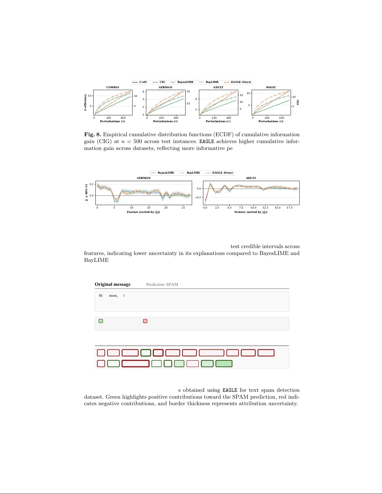
Leave a Comment