Free Final Time Adaptive Mesh Covariance Steering via Sequential Convex Programming

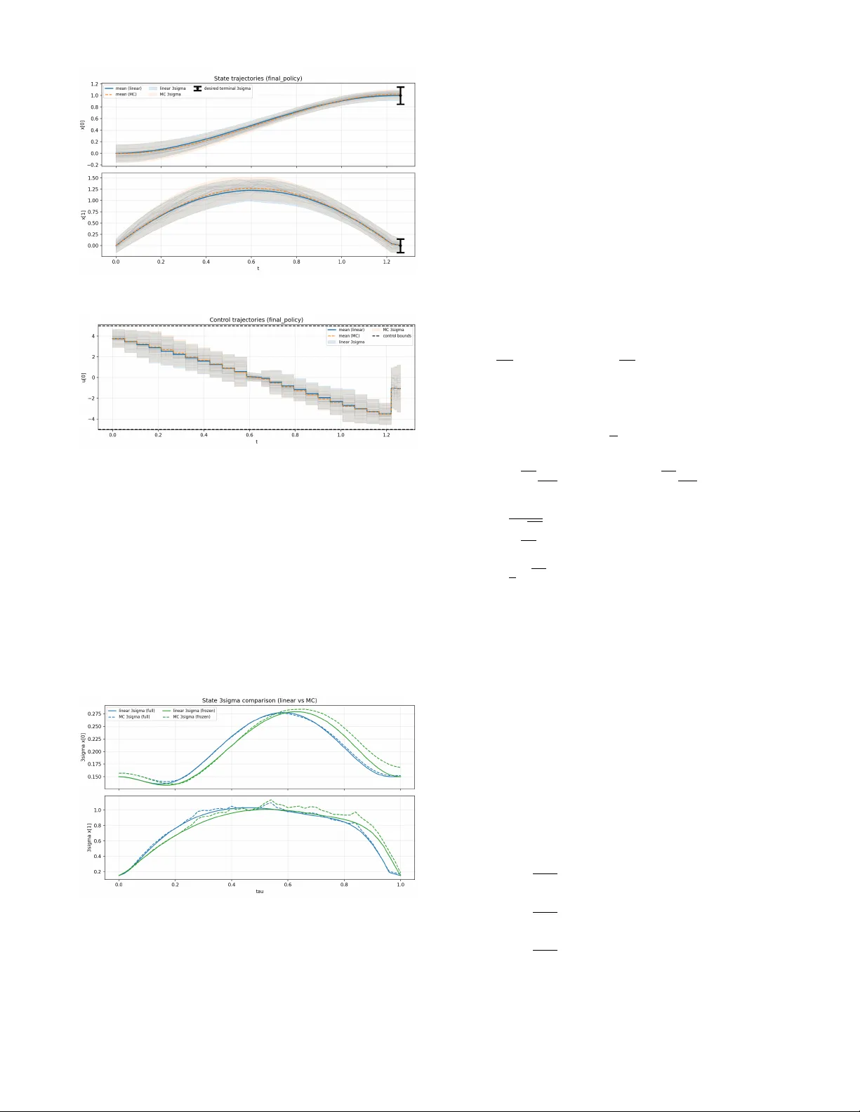
Fr ee Final T ime Adaptiv e Mesh Cov ariance Steering via Sequential Con vex Pr ogramming Joshua Pilipovsk y Abstract — In this paper we develop a sequential-con vex- programming (SCP) framework for free-final-time covariance steering of nonlinear stochastic differential equations (SDEs) subject to both additive and multiplicative diffusion. W e cast the free-final-time objectiv e through a time-normalization and introduce per -interv al time-dilation variables that induce an adaptive discretization mesh, enabling the simultaneous op- timization of the control policy and the temporal grid. A central difficulty is that, under multiplicative noise, accurate covariance propagation within SCP r equires retaining the first-order diffusion linearization and its coupling with time dilation. W e theref ore derive the exact local linear stochastic model (preserving the multiplicative structure) and introduce a tractable discretization that maintains the associated diffu- sion terms, after which each SCP subproblem is solved via conic/semidefinite covariance-steering relaxations with termi- nal moment constraints and state/contr ol chance constraints. Numerical experiments on a nonlinear double-integrator with drag and v elocity-dependent diffusion validate free-final-time minimization through adaptive time allocation and improved covariance accuracy relative to frozen-diffusion linearizations. I . I N T R O D U C T I O N Successiv e con vexification (SCvx) and, more broadly , se- quential con vex programming (SCP) methods have become a leading paradigm for noncon vex optimal control due to their polynomial-time conv ex subproblems, strong empirical reliability , and increasingly mature con vergence/feasibility guarantees [1], [2], [3]. In aerospace guidance and trajectory optimization, these methods hav e enabled real-time-capable pipelines for problems with nonlinear dynamics, noncon ve x state/control constraints, and free-final-time objectiv es [4]. In their standard form, SCvx discretizes the continuous-time problem on a fixed temporal mesh, con ve xifies the dynamics and noncon vex constraints about a reference trajectory , and enforces progress through trust-region and penalty mecha- nisms (e.g., virtual controls and constraint softening). Extending this paradigm to stochastic optimal control is substantially more challenging because one must simulta- neously steer the mean trajectory and propagate/control un- certainty under probabilistic safety requirements. Cov ariance control (and, in finite horizon form, cov ariance steering (CS)) addresses this by shaping the first two moments of the state distribution via feedback control, and has led to conv ex, scalable synthesis methods for linear stochastic systems with terminal cov ariance and chance constraints [5], [6], [7], [8]. These de velopments have supported a growing body of constrained stochastic guidance applications, including J. Pilipovsky is a Senior Research Engineer at R TX T echnology Research Center (R TRC), East Hartford, CT , 06119, USA. Email: joshua.y .pilipovsky@rtx.com spacecraft proximity operations and lo w-thrust trajectory design [9], [10], [11]. A natural next step is to combine the tractability and relia- bility of SCvx with the distribution-shaping guarantees of CS for nonlinear stochastic systems. Iterati ve co v ariance steering (iCS) [10], [12], [13], [14] follows this strate gy by repeatedly linearizing a nonlinear stochastic dif ferential equation (SDE), solving a con ve x CS subproblem for the local model, and up- dating the reference within an SCP loop. For additiv e noise, local cov ariance propagation is relativ ely straightforward; howe ver , many applications are more naturally modeled with multiplicative noise, where the diffusion depends on the state and/or control (e.g., atmospheric-density-dri ven entry uncertainty , attitude-dependent disturbances, and throttle- /pointing-dependent propulsion uncertainty). In this setting, cov ariance dynamics depend on the first-order diffusion linearization, and the resulting CS constraints can become noncon vex unless suitable liftings/relaxations are introduced [15], [16]. Moreo ver , within SCP/iCS, mismatch between the cov ariance propagation used in the conv ex subproblem and the true local stochastic dynamics can accumulate and degrade constraint satisfaction and conv ergence. Many guidance and mission-design problems are also intrinsically fr ee-final-time . In deterministic SCvx, this is commonly handled by time normalization and a time-dilation variable, which preserves a fixed number of discretization nodes while introducing a con vex surrogate for final time [4]. Adaptiv e-mesh SCP variants further generalize this idea by optimizing interval-wise time dilation or reallocating discretization density [17], [3], [18], [19]. In stochastic problems, ho we ver , time dilation scales not only the drift but also the diffusion, and therefore directly af fects covariance growth. T o our knowledge, a principled CS formulation that jointly optimizes the temporal mesh and the cov ariance steering policy for nonlinear SDEs with multiplicative noise has not been pre viously dev eloped. The purpose of this paper is to close this gap. W e consider a nonlinear continuous-time SDE with control-affine (possibly nonlinear) drift and state/control- dependent diffusion, subject to terminal mean/cov ariance requirements and con vex chance constraints along the trajec- tory , and seek a feedback polic y that minimizes final time . W e time-normalize the dynamics to τ ∈ [0 , 1] and introduce per- interval time-dilation variables { σ k } N − 1 k =0 , which induce an adaptiv e physical-time mesh while keeping the normalized discretization fix ed. A key technical ingredient is a first- order discretization of the local linear multiplicativ e-noise model that preserves the diffusion linearization including its time-dilation dependence , together with one-step mean- square error bounds. This yields more accurate co v ariance propagation inside the SCP loop under multiplicative noise and enables the integration of lossless conv ex relaxations for multiplicativ e-noise CS within each con ve x subproblem. Contributions The main contributions of this work are as follows. 1) T o the authors’ knowledge, the first free-final-time cov ariance-steering formulation for nonlinear SDEs, using interv al-wise time-dilation v ariables to jointly optimize the control policy and temporal mesh within an SCP/iCS framew ork. 2) An exact first-order dif fusion linearization under time normalization (including time-dilation coupling), to- gether with a discrete-time local stochastic model and mean-square error bounds that support accurate cov ariance propagation under multiplicati ve noise. 3) A tractable SCvx ⋆ -based solution method whose con- ve x subproblems incorporate lossless conv ex relax- ations for multiplicati ve-noise covariance steering and con vex chance constraints, demonstrated on a nonlin- ear double-integrator example with drag and velocity- dependent diffusion. I I . N O T A T I O N All random objects are defined on a common proba- bility space (Ω , F , P ) . Deterministic vectors are denoted by lowercase letters ( u ∈ R m ), matrices by uppercase letters ( V ∈ R n × m ), and random vectors by boldface ( x ∈ R n ). W e denote the sets of symmetric, posi- tiv e semidefinite, and positiv e definite matrices by S n , S n + , and S n ++ , respecti vely . A continuous-time signal o ver t ∈ [ t 0 , t 1 ] is written { x t } t ∈ [ t 0 ,t 1 ] . Given a filtration {F τ } τ ≥ 0 , we write E k [ · ] : = E [ · | F τ k ] . For ζ ∈ R r , [ ζ ] + : = [max( ζ 1 , 0) , . . . , max( ζ r , 0)] ⊺ represents the vec- torized maximum. For non-negati ve quantities a and b , we write a ≲ b if there exists a finite constant C > 0 such that a ≤ C b. Finally , [ a ; b ] and [ A ; B ] denote vertical concatenation of compatible vectors and matrices. I I I . P R O B L E M S T A T E M E N T Consider a dynamical system governed by the nonlinear stochastic differential equation (SDE) d x t = f  x t , u t  d t + g  x t , u t  d w t , t ∈ [0 , t f ] , (1) where x t ∈ R n is the state, u t ∈ R m is the control input, w t ∈ R d is a d -dimensional Brownian motion, and t f > 0 is the final time. In this work, we assume that t f is fr ee . The state is initially normally distributed as x 0 ∼ N ( µ i , Σ i ) , (2) where µ i ∈ R n and Σ i ∈ S n ++ , and the terminal distribution is constrained to be x t f ∼ N ( µ f , Σ f ) , (3) where µ f ∈ R n and Σ f ∈ S n ++ . Let X ⊂ R n and U ⊂ R m denote the allow able conv ex sets for state and input, which we assume are giv en by the polytopes X = N x \ j =1 { x : α ⊺ j x + β j ≤ 0 } , U = N u \ j =1 { u : a ⊺ j u + b j ≤ 0 } , (4) where α j ∈ R n , a j ∈ R m and β j , b j ∈ R define the indi- vidual half-spaces. The above choice is for simplicity; other con vex (e.g., norm-based) or even nonconv ex (e.g., obstacle- av oidance) admissible regions can be handled within the SCP framew ork in Section V [13], [20]. W e impose continuous- time joint chance constraints P ( x t ∈ X ∀ t ∈ [0 , t f ]) ≥ 1 − ∆ x , (5a) P ( u t ∈ U ∀ t ∈ [0 , t f ]) ≥ 1 − ∆ u , (5b) where ∆ x , ∆ u ∈ (0 , 0 . 5] are joint risk tolerances. W e consider an objective function which aims to minimize the regularized final time J ( x , u , t f ) = η t f + J reg ( x , u ) , (6) where η > 0 weighs the free-final time, and J reg ≥ 0 denotes a mean/covariance regularization which will be precisely defined in Section IV -G. W e define the set π of admissi- ble control inputs as the set of (random) control signals { u t } t ∈ [0 ,t f ] where the input u t is an affine function of the state. In total, the F ree-Final T ime C ov ariance S teering (FFT -CS) is giv en as follows Pr oblem 1 (FFT -CS): For a giv en initial distrib ution (2), find a control policy that minimizes (6) subject to (1) and (5), such that (3) holds. I V . P RO B L E M R E F O R M U L A T I O N T o find a locally optimal solution to Problem 1, we utilize the frame work of Sequential Con vex Programming (SCP), which aims to iterati vely build and solve approximate (yet tractable) con ve x sub-problems of Problem 1. The ov erall iterativ e scheme is presented in Algorithm 1 and is discussed in detail in Section V. In this section, we outline the main steps that must be performed to arriv e at a tractable con ve x CS sub-problem, namely (i) time scaling, (ii) linearization, (iii) discretization, and (iv) con vex reduction. A. T ime Scaling Since the final time t f is free, it is con venient (and in this context, necessary) to scale the time horizon [0 , t f ] to a fix ed interv al. Let t : [0 , 1] → [0 , t f ] be a continuously differentiable and nondecreasing function of a parameter τ with t (0) = 0 and t (1) = t f , and define the time-dilation factor σ τ : = d t/ d τ ≥ 0 . Under this change of v ariables, the dynamics (1) are equiv alently written on the fixed interv al τ ∈ [0 , 1] as d x τ = σ τ f ( x τ , u τ ) d τ + √ σ τ g ( x τ , u τ ) d w τ . (7) Moreov er , it is straightforward to see that t f = Z 1 0 σ τ d τ , (8) so the objectiv e (6) is equiv alently written as J ( x , u , σ ) = η Z 1 0 σ τ d τ + J reg ( x , u ) . (9) The nonlinear SDE (7) and objective (9) are no w written ov er a fixed horizon, at the cost of introducing the additional decision v ariable σ τ . This time scaling procedure, which is now customary in deterministic optimal control SCP algo- rithms [4], [3], [21], has scarcely been applied to stochastic optimal control problems. Throughout, the normalized state process { x τ } τ ∈ [0 , 1] is assumed adapted to the natural filtration F τ : = σ  x 0 , { w s : 0 ≤ s ≤ τ }  , τ ∈ [0 , 1] , (10) generated by the initial condition x 0 and the driving Bro w- nian motion d w τ . For con venience, explicit expressions for the linearization and discretization matrices that appear in the sequel are collected in Appendix A and Appendix B. B. Linearization W e linearize (7) about a reference trajectory ˆ z τ : = ( ˆ x τ , ˆ u τ , ˆ σ τ ) . For clarity , write the diffusion column-wise as g = [ g 1 , . . . , g d ] ∈ R n × d . Define the augmented control input ˜ u τ : = [ u ⊺ τ , σ τ ] ⊺ ∈ R m +1 and the matrices F τ : =  B τ c τ  , ˜ F ( i ) τ : = h ˜ B ( i ) τ ˜ c ( i ) τ i . Then the first-order It ˆ o linearization yields d x τ = ( A τ x τ + F τ ˜ u τ + d τ ) d τ + d X i =1  ˜ A ( i ) τ x τ + ˜ F ( i ) τ ˜ u τ + ˜ d ( i ) τ  d w ( i ) τ . (11) The matrices and vectors in volved in this linearization are giv en e xplicitly in Appendix A. Remark 1: In contrast to prior SCP/iCS formulations [13], [14], [10], [12] that freeze the diffusion at the reference (i.e., ˜ A ( i ) τ = ˜ F ( i ) τ = 0 ), (11) retains the full first-order dif fusion linearization, including the time-dilation dependence through √ σ τ . This yields more accurate local moment propagation inside SCP , at the cost of a multiplicativ e-noise linear model (and hence generally non-Gaussian state distributions). C. Discr etization W e discretize (11) on a partition P : = ( τ 0 , . . . , τ N ) with τ 0 = 0 , τ N = 1 and step sizes ∆ τ k : = τ k +1 − τ k . It is important to note that ev en if the time-scaled step size is fixed, i.e., ∆ τ k ≡ ∆ τ , the physical time step need not be constant, since ∆ t k = R ∆ τ 0 σ τ d τ . For brevity , we write x t k = x k , u t k = u k , and so on for all other decision v ariables. W e assume a zero-order hold (ZOH) on the augmented control input, that is, ˜ u τ ≡ ˜ u k , ∀ τ ∈ [ τ k , τ k +1 ) . (12) Under ZOH on σ τ , the objectiv e (9) is approximated by the Riemann sum J ( x k , ˜ u k ) ≈ η N − 1 X k =0 σ k ∆ τ k + J reg ( x k , u k ) , (13) which is linear in the decision variables { σ k } . Let Φ( τ , s ) denote the state transition matrix (STM) associated with ˙ z = A τ z , i.e., ∂ ∂ τ Φ( τ , s ) = A τ Φ( τ , s ) , Φ( s, s ) = I . (14) Under the ZOH assumption (12), the linear SDE (11) admits the exact mild solution on [ τ k , τ k +1 ] : x k +1 = A k x k + ν k + d X i =1 Z τ k +1 τ k Φ( τ k +1 , τ )  ˜ A ( i ) τ x τ + ˜ ν ( i ) τ  d w ( i ) τ , (15) where ν k : = F k ˜ u k + d k , ˜ ν ( i ) τ : = ˜ F ( i ) τ ˜ u k + ˜ d ( i ) τ . The deterministic discretization terms ( A k , F k , d k ) together with the averaged diffusion coef ficients ( ˜ A ( i ) k , ˜ F ( i ) k , ˜ d ( i ) k ) are giv en in Appendix B. Therein, we also present a computationally efficient (and parallelizable) procedure to compute these matrices by solving a small augmented linear ODE, av oiding per-interv al numerical quadrature. The only intractable term in (15) is the stochastic integral, since x τ appears inside the integrand. In the follo wing, we ov ercome this issue by (i) freezing the state inside the integrand and (ii) approximating with a constant integrand. Assumption 1 (F r ozen state in the diffusion inte grand): On each interval [ τ k , τ k +1 ] , we approximate the diffusion integrand in (15) by freezing the state at the left endpoint: x τ ≈ x k , ∀ τ ∈ [ τ k , τ k +1 ] . (16) For each channel i ∈ { 1 , . . . , d } and τ ∈ [ τ k , τ k +1 ] , define the F τ k -measurable integrand H k,i ( τ ; x k , ˜ u k ) : = Φ( τ k +1 , τ )  ˜ A ( i ) τ x k + ˜ ν ( i ) τ  ∈ R n . (17) Stack the channels as H k ( τ ; x k , ˜ u k ) : =  H k, 1 ( τ ) · · · H k,d ( τ )  ∈ R n × d , (18) ∆ w k : =  ∆ w k, 1 · · · ∆ w k,d  ⊺ ∈ R d , (19) where ∆ w k,i : = w ( i ) τ k +1 − w ( i ) τ k and hence ∆ w k ∼ N (0 , ∆ τ k I d ) with statistics E [∆ w k ] = 0 , E [∆ w k ∆ w ⊺ k ] = ∆ τ k I d . (20) Moreov er , since x k is F τ k -measurable and Bro wnian incre- ments are independent of F τ k , we have ∆ w k ⊥ ⊥ F τ k (and hence ∆ w k is independent of x k ). Furthermore, define the av eraged (projected) integrand ¯ H k ( x k , ˜ u k ) : = 1 ∆ τ k Z τ k +1 τ k H k ( τ ; x k , ˜ u k ) d τ ∈ R n × d . (21) W e approximate the It ˆ o integral in (15) by the constant- integrand It ˆ o integral as Z τ k +1 τ k H k ( τ ; x k , ˜ u k ) d w τ ≈ Z τ k +1 τ k ¯ H k ( x k , ˜ u k ) d w τ = ¯ H k ( x k , ˜ u k ) ∆ w k . (22) Note that ¯ H k ( · ) ∈ R n × d is column-wise af fine in ( x k , ˜ u k ) , i.e., for each channel i , ¯ H k,i ( x k , ˜ u k ) = ˜ A ( i ) k x k + ˜ F ( i ) k ˜ u k + ˜ d ( i ) k . (23) Combining Assumption 1 with (22), we obtain the tractable discrete-time approximation of (15) x k +1 ≈ A k x k + ν k + ¯ H k ( x k , ˜ u k ) ∆ w k . (24) The approximation (22) is optimal (in conditional mean- square) within the class of constant integrands; see Ap- pendix C. Naturally , one may wonder how much error the abov e approximation scheme incurs compared to exact discretization. W e now formalize one-step mean-square error bounds for (i) freezing x τ 7→ x k inside the diffusion integrand, and (ii) projecting the frozen It ˆ o inte gral onto ¯ H k ∆ w k . Theor em 1 (One-step diffusion discr etization error): Fix the time step k ∈ { 0 , . . . , N − 1 } and consider the exact mild update x ex k +1 in (15). Let x fr k +1 : = A k x k + ν k + Z τ k +1 τ k H k ( τ ; x k , ˜ u k ) d w τ , denote the fr ozen state update, and let x ap k +1 denote the pr ojected (fully approximated) state update in (24). Denote the associated errors e ( x ) k +1 : = x ex k +1 − x fr k +1 (freezing) and e ( p ) k +1 : = x fr k +1 − x ap k +1 (projection). Assume Assumption 2 (in Appendix D) holds on T k = [ τ k , τ k +1 ] . Then the conditional mean-square errors satisfy E k h ∥ e ( x ) k +1 ∥ 2 i ≲ ∆ τ 2 k  1 + ∥ x k ∥ 2 + ∥ ˜ u k ∥ 2  , (25a) E k h ∥ e ( p ) k +1 ∥ 2 i ≤ 1 12 L H,k ( x k , ˜ u k ) 2 ∆ τ 3 k , (25b) where L H,k ( x k , ˜ u k ) is the one-step time-Lipschitz modulus of the map τ 7→ H k ( τ ; x k , ˜ u k ) . Pr oof: See Appendix E. Remark 2: For small steps, the freezing error is O (∆ τ 2 k ) while the projection error is O (∆ τ 3 k ) . Hence, the freezing er- ror dominates the diffusion discretization error in the present scheme. Compared to existing methods [12], [10] that freeze the diffusion at the current reference before linearization, which incurs an error O (∆ τ ) , the proposed method which performs exact first-order linearization but approximate dis- cretization has an error an order-of-magnitude smaller . D. Moment Pr opagation T o encode the mean and covariance constraints (3) as well as reformulate the chance constraints (5), it is necessary to propagate the mean and covariance of the state. W e first expand the discretized dynamics (24) into a more familiar form to facilitate the analysis. T o this end, note the following equiv alence x k +1 = A k x k + ν k + d X i =1  ˜ A ( i ) k x k + ˜ ν ( i ) k  ∆ w ( i ) k = A k x k + F k ˜ u k + D k , (26) where A k : = A k + P d i =1 ˜ A ( i ) k ∆ w ( i ) k , F k : = F k + P d i =1 ˜ F ( i ) k ∆ w ( i ) k , and D k : = d k + P d i =1 ˜ d ( i ) k ∆ w ( i ) k . Struc- turally , the resultant dynamical system (26) is that of a linear system perturbed by (correlated) multiplicative and additi ve noise. Next, and similar to the deri vation in [16], we compute the first two moments of the uncertain affine system (26). Theor em 2 (One-step moment pr opagation): Let ¯ x k : = E [ x k ] denote the mean state and let Σ x k : = E [( x k − ¯ x k )( x k − ¯ x k ) ⊺ ] , Σ x k ˜ u k : = E [( x k − ¯ x k )( ˜ u k − E [ ˜ u k ]) ⊺ ] , Σ ˜ u k : = E [( ˜ u k − E [ ˜ u k ])( ˜ u k − E [ ˜ u k ]) ⊺ ] denote the state co v ariance, state–control cross covariance, and control cov ariance, respectively . Then the one-step mean and cov ariance propagation associated with (26) is ¯ x k +1 = A k ¯ x k + F k E [ ˜ u k ] + d k , (27a) Σ x k +1 = A k Σ x k A ⊺ k + A k Σ x k ˜ u k F ⊺ k + F k Σ ⊺ x k ˜ u k A ⊺ k + F k Σ ˜ u k F ⊺ k + ∆ τ k d X i =1  ˜ A ( i ) k Σ x k ( ˜ A ( i ) k ) ⊺ + ˜ A ( i ) k Σ x k ˜ u k ( ˜ F ( i ) k ) ⊺ + ˜ F ( i ) k Σ ⊺ x k ˜ u k ( ˜ A ( i ) k ) ⊺ + ˜ F ( i ) k Σ ˜ u k ( ˜ F ( i ) k ) ⊺ + q ( i ) k ( q ( i ) k ) ⊺  , (27b) where q ( i ) k : = ˜ A ( i ) k ¯ x k + ˜ F ( i ) k E [ ˜ u k ] + ˜ d ( i ) k . Pr oof: See Appendix F. E. P olicy parameterization W e employ affine state-deviation feedback of the form ˜ u k = ˜ v k + ˜ K k ( x k − ¯ x k ) , (28) where ˜ v k : = [ v k ; σ k ] ∈ R m +1 and ˜ K k : = [ K k ; 0 1 × n ] ∈ R ( m +1) × n . Under the parameterization (28), the statistics of the control input satisfy E [ ˜ u k ] = ˜ v k , Σ ˜ u k = ˜ K k Σ x k ˜ K ⊺ k , and Σ x k ˜ u k = Σ x k ˜ K ⊺ k . Substituting into (27) yields ¯ x k +1 = A k ¯ x k + F k ˜ v k + d k , (29a) Σ x k +1 = ( A k + F k ˜ K k ) Σ x k ( A k + F k ˜ K k ) ⊺ + ∆ τ k · d X i =1  ( ˜ A ( i ) k + ˜ F ( i ) k ˜ K k ) Σ x k ( ˜ A ( i ) k + ˜ F ( i ) k ˜ K k ) ⊺ + q ( i ) k ( q ( i ) k ) ⊺  . (29b) From the resulting moment propagation in (29), it is apparent that the mean dynamics (29a) are linear in the decision variables { ¯ x k , v k , σ k } . Equation (29b), on the other hand, makes explicit the nonlinear coupling between Σ x k and ˜ K k . This issue will be resolv ed in Section IV -G through a suitable lossless relaxation. F . Chance Constraints Because the exact diffusion linearization induces multi- plicativ e noise, the discretized local model (24) is generally non-Gaussian ev en for Gaussian initial conditions. W e there- fore enforce chance constraints through a sufficient distribu- tionally robust surrogate based only on the propagated first two moments (27), namely the distributionally rob ust chance constraints (DR-CC) inf P x τ ∈C ( µ τ , Σ x τ ) P x τ ( x t ∈ X , ∀ τ ∈ [0 , 1]) ≥ 1 − ∆ x , (30a) inf P u τ ∈C ( v τ , Σ u τ ) P u τ ( u τ ∈ U , ∀ τ ∈ [0 , 1]) ≥ 1 − ∆ u , (30b) where C ( µ, Σ) denotes the Chebyshev ambiguity set of all distributions whose first two moments are equal to ( µ, Σ) . W e enforce (30) at the grid nodes τ k (rather than con- tinuously in time); continuous-time DR-CC enforcement via isoperimetric reformulations is possible [3] but omitted here. Using the polytopic sets in (4), we impose inf P x k ∈C ( µ k , Σ x k ) P x k ( α ⊺ j x k + β j ≤ 0 , ∀ j, k ) ≥ 1 − ∆ x , (31a) inf P u k ∈C ( v k , Σ u k ) P u k ( a ⊺ j u k + b j ≤ 0 , ∀ j, k ) ≥ 1 − ∆ u . (31b) The joint DR-CC in (31) are non-conv ex and intractable, in general [20]. W e employ a standard relaxation using Boole’ s inequality [22] to reformulate the joint DR-CC as the individual DR-CC inf P x k ∈C ( µ k , Σ x k ) P x k ( α ⊺ j x k + β j ≤ 0) ≥ 1 − δ x j,k , (32a) inf P u k ∈C ( v k , Σ u k ) P u k ( a ⊺ j u k + b j ≤ 0) ≥ 1 − δ u j,k , (32b) N x X j =1 N X k =1 δ x j,k ≤ ∆ x , N u X j =1 N − 1 X k =0 δ u j,k ≤ ∆ u , (32c) where δ x j,k , δ u j,k ∈ (0 , 0 . 5] represent the state and input risk allocations, respectively . In general, these variables are unknown and must be optimized jointly with that of the state and control variables at run-time. Ho we ver , in this work, we employ the standard approximation of fixing the risk variables to the constant allocation δ x j,k = ∆ x / ( N N x ) and δ u j,k = ∆ u / ( N N u ) . W e remark, ho we ver , that it is possible to jointly optimize the risk allocation with the controller using a two-step approach [23], [9]. Finally , we use results from the distributionally robust optimization literature [24] to e valuate the minimization problems in (32) in closed form, yielding α ⊺ j µ k + β j + Q ( δ x j,k ) q α ⊺ j Σ x k α j ≤ 0 , (33a) a ⊺ j v k + b j + Q ( δ u j,k ) q a ⊺ j Σ u k a j ≤ 0 , (33b) where Q ( δ ) ≜ p δ − 1 (1 − δ ) . G. Con vex reduction W e now reformulate the non-conv ex constraints in the co- variance propagation and distributionally robust (DR) chance constraints into a tractable con vex form suitable for SCP subproblems. Specifically , the one-step covariance recursion (29b) contains (i) nonlinear terms coupling the covariance and feedback variables (Σ x k , ˜ K k ) , and (ii) quadratic outer- product terms coupling the mean and feedforward v ariables ( ¯ x k , ˜ v k ) . In addition, the DR chance constraints (33) are non- con vex due to the square-root dependence on the state and input cov ariances. W e address the cov ariance-recursion non- con vexities via lifting and Schur-complement relaxations, and then conv exify the chance constraints through auxiliary variables and first-order linearization. The resulting con- straints are conic/semidefinite representable and therefore compatible with the SCP subproblems. Nonlinearity in (Σ x k , ˜ K k ) : In a similar vein to [8], we introduce the change of variables U k : = ˜ K k Σ x k ∈ R ( m +1) × n . (34) Whenev er Σ x k ≻ 0 , we ha ve ˜ K k = U k Σ − 1 x k and hence ˜ K k Σ x k ˜ K ⊺ k = U k Σ − 1 x k U ⊺ k , (35) which is jointly noncon ve x in ( U k , Σ x k ) . W e con vexify via the LMI relaxation Y k ⪰ U k Σ − 1 x k U ⊺ k . (36) Using the Schur complement (and the fact that Σ x k ≻ 0 ), (36) is equiv alent to  Y k U k U ⊺ k Σ x k  ⪰ 0 . (37) Bilinearity in ( ¯ x k , ˜ v k ) : For each ( i, k ) , define the auxiliary decision variable ˜ Σ ik ⪰ ˜ q ( i ) k ( ˜ q ( i ) k ) ⊺ , ˜ q ( i ) k = ˜ A ( i ) k ¯ x k + ˜ F ( i ) k ˜ v k + ˜ d ( i ) k . (38) Again by the Schur complement, (38) is equiv alent to the LMI " ˜ Σ ik ˜ q ( i ) k ( ˜ q ( i ) k ) ⊺ 1 # ⪰ 0 . (39) Substituting (34)–(39) into the cov ariance propagation (29b) yields the following con vex constraint system Σ x k +1 = A k Σ x k A ⊺ k + A k U ⊺ k F ⊺ k + F k U k A ⊺ k + F k Y k F ⊺ k + ∆ τ k d X i =1  ˜ A ( i ) k Σ x k ( ˜ A ( i ) k ) ⊺ + ˜ A ( i ) k U ⊺ k ( ˜ F ( i ) k ) ⊺ + ˜ F ( i ) k U k ( ˜ A ( i ) k ) ⊺ + ˜ F ( i ) k Y k ( ˜ F ( i ) k ) ⊺ + ˜ Σ ik  , (40a)  Y k U k U ⊺ k Σ x k  ⪰ 0 , (40b)  ˜ Σ ik ˜ A ( i ) k ¯ x k + ˜ F ( i ) k ˜ v k + ˜ d ( i ) k ⋆ 1  ⪰ 0 , ∀ i ∈ { 1 , . . . , d } , (40c) for all time steps k = 0 , . . . , N − 1 . The con- straints in (40) are af fine in the decision variables { ¯ x k , Σ x k , ˜ v k , U k , Y k , ˜ Σ ik } . It is natural to ask whether the relaxations (36) and (38) introduce conserv atism in the cov ariance propagation and, consequently , in the terminal co- variance constraints (3). In general, (40a) over -approximates the one-step covariance. Let P k denote the true state co- variance under the linearized dynamics (29b). Then Σ x k ⪰ P k for all k = 0 , . . . , N (with equality at k = 0 ), so enforcing Σ x N = Σ f is sufficient to guarantee P N ⪯ Σ f . Moreov er , with a suitable regularization of the objective (13), the relaxations become lossless at optimality; i.e., the relaxed and original cov ariance-steering problems share the same optimal decision v ariables and objecti ve v alue (see Theorem 3, Appendix G). Next, we conv exify the DR chance constraints (33). W e first relax the input-cov ariance terms by replacing Σ u k with Y k . Since Y k ⪰ Σ u k , this yields sufficient (generally conservati ve) input constraints. W e then introduce auxiliary variables κ x,j,k , κ u,j,k ≥ 0 satisfying κ 2 x,j,k ≥ α ⊺ j Σ x k α j , κ 2 u,j,k ≥ a ⊺ j Y k a j . Under this lifting, the DR chance constraints become linear in ( µ k , v k , κ x,j,k , κ u,j,k ) , while the remaining non-conv exity is isolated in the quadratic inequalities defining κ x,j,k and κ u,j,k . Gi ven reference values ( ˆ κ x,j,k , ˆ κ u,j,k ) (initialized as discussed in Section V), we linearize these inequalities to obtain α ⊺ j ¯ x k + β j + Q ( δ x j,k ) κ x,j,k ≤ 0 , (41a) α ⊺ j Σ x k α j − ˆ κ 2 x,j,k − 2 ˆ κ x,j,k ( κ x,j,k − ˆ κ x,j,k ) ≤ 0 , (41b) a ⊺ j v k + b j + Q ( δ u j,k ) κ u,j,k ≤ 0 , (41c) a ⊺ j Y k a j − ˆ κ 2 u,j,k − 2 ˆ κ u,j,k ( κ u,j,k − ˆ κ u,j,k ) ≤ 0 . (41d) Finally , for completeness we note that the initial and terminal distributional constraints on the state are conv ex by design, since we assume the moments are decision variables in the resulting program. As a result, the boundary moment constraints are simply written as ¯ x 0 = µ i , Σ x 0 = Σ i , (42a) ¯ x N = µ f , Σ x N = Σ f . (42b) V . S E Q U E N T I A L C O N V E X P R O G R A M M I N G In this section, we present the full FFT -iCS SCP pro- cedure used to compute a local solution of Problem 1. At iteration ℓ , the nonlinear time-scaled SDE is linearized and discretized about a current reference, the resulting con vex penalty cov ariance-steering subproblem is solved, and the candidate step is accepted or rejected according to the standard SCvx ⋆ ratio test. In the following, we state the initialization, diagnostics, and update formulas explicitly . The first step is to construct an initial reference trajectory and time-dilation profile ( ˆ x (0) , ˆ u (0) , ˆ σ (0) ) for the system linearization. This initialization is problem dependent; in practice, any boundary-consistent deterministic or mean-only steering solution, or any near-feasible interpolating trajectory with admissible control and mesh v ariables, may be used. Giv en ( ˆ x (0) , ˆ u (0) , ˆ σ (0) ) , the remaining chance-constraint lin- earization variables are initialized from a preliminary un- constrained FFT -CS solve 1 , exactly as in [10]. From the resulting cov ariances { Σ ⋆ x k , Y ⋆ k } , we set ˆ κ (0) x,j,k = q α ⊺ j Σ ⋆ x k α j , ˆ κ (0) u,j,k = q a ⊺ j Y ⋆ k a j . T ogether with the remaining primal v ariables produced by the warm start, this yields the full reference tuple ˆ z (0) for Problem 2. W e denote by ˆ y ( ℓ ) : =  ˆ x ( ℓ ) , ˆ u ( ℓ ) , ˆ σ ( ℓ ) , ˆ κ ( ℓ )  1 This can be interpreted as a zeroth (warm-start) iteration. In practice, the corresponding optimal decision variables may also be passed as the initial guess for the first chance-constrained solve, which often improves solver con ver gence. the subset of ˆ z ( ℓ ) required for linearization and discretization. The associated local model data are summarized by Z ( ℓ ) = dis P ◦ lin D ( ˆ y ( ℓ ) ) , where D denotes the time-scaled nonlinear system (7) and P the partition in (24). There are two well-kno wn pathologies of SCP subprob- lems: (i) artificial infeasibility and (ii) artificial unbounded- ness . T o address the former, we introduce virtual controls / buffer variables in the linearized constraints and penalize them in the objective. T o address the latter , we impose trust-region constraints around the current linearization point. Specifically , we soften the linearized mean dynamics and the linearized chance-constraint quadratic surrogates via ¯ x k +1 − A k ¯ x k − F k ˜ v k − d k = ξ k , (43a) α ⊺ j Σ x k α j − 2 ˆ κ x,j,k κ x,j,k + ˆ κ 2 x,j,k ≤ ζ x,j,k , (43b) a ⊺ j Y k a j − 2 ˆ κ u,j,k κ u,j,k + ˆ κ 2 u,j,k ≤ ζ u,j,k , (43c) where ξ k ∈ R n and ζ x,j,k , ζ u,j,k ≥ 0 are penalized using the augmented-Lagrangian penalty [2] J pen ( ξ , ζ | w , λ, µ ) = µ ⊺ ξ + w 2 ∥ ξ ∥ 2 2 + λ ⊺ ζ + w 2 ∥ [ ζ ] + ∥ 2 2 , (44) with multipliers µ ∈ R N n and λ ∈ R ( N x + N u ) N and penalty weight w > 0 . Artificial unboundedness is mitigated by the trust region         W x W ˜ u W κ     ¯ x − ˆ x ˜ v − [ ˆ u ; ˆ σ ] κ − ˆ κ         ∞ ≤ ∆ tr , (45) where W x , W ˜ u , W κ ≻ 0 are scaling matrices and ∆ tr > 0 is the trust-region radius. Putting these ingredients together , the con ve x penalty cov ariance-steering subproblem solved at each SCP iteration is the following. Pr oblem 2 (P-CS): Let the primal decision v ariables be z : =  { ¯ x k } N k =0 , { Σ x k } N k =0 , { ˜ v k } N − 1 k =0 , { U k , Y k } N − 1 k =0 , { ˜ Σ ik } d, N − 1 i =1 ,k =0 , { κ x,j,k } N x , N j =1 ,k =1 , { κ u,j,k } N u , N − 1 j =1 ,k =0  , and define the penalty variables ξ := { ξ k } N − 1 k =0 , ζ :=  { ζ x,j,k } N x , N j =1 ,k =1 , { ζ u,j,k } N u , N − 1 j =1 ,k =0  . Define L := R n × S n ++ × R m × R + × R ˜ m × n × S ˜ m + × S n + × R N x + × R N u + as the per-stage feasible cone, where ˜ m = m + 1 . The penalty cov ariance-steering problem is min z ,ξ,ζ η N − 1 X k =0 ∆ τ k σ k + J reg ( z ) + J pen ( ξ , ζ ) s.t. (43a) ← soft mean constraints (40) ← covariance constraints (41a) , (41c) , (43b) , (43c) ← soft chance constraints (45) ← trust re gion constraints (42) ← boundary constraints z ∈ L , ξ ∈ R N n , ζ ∈ R ( N x + N u ) N + . T o define the SCvx ⋆ diagnostics, let J ( ℓ ) nl ( z ) : = J ( z ) + J pen  g nl ( z ) , h nl ( z ) | w ( ℓ ) , λ ( ℓ ) , µ ( ℓ )  , (46a) L ( ℓ ) cvx ( z , ξ , ζ ) : = J ( z ) + J pen  ξ , ζ | w ( ℓ ) , λ ( ℓ ) , µ ( ℓ )  , (46b) where, for all k = 0 , . . . , N − 1 , the nonlinear residual maps are giv en by g nl ,k ( z ) : = ¯ x k +1 −  ¯ x k + Z τ k +1 τ k σ k f ( ¯ x τ , v k ) d τ  , h nl ,x,j,k ( z ) : = α ⊺ j Σ x k +1 α j − κ 2 x,j,k +1 , j = 1 , . . . , N x , h nl ,u,j,k ( z ) : = a ⊺ j Y k a j − κ 2 u,j,k , j = 1 , . . . , N u , and g nl ( z ) and h nl ( z ) collect these equality and inequality residuals, respectiv ely . Thus, after solving Problem 2 at itera- tion ℓ and obtaining ( z ⋆ , ξ ⋆ , ζ ⋆ ) , we define the nonlinear cost improv ement, linearized cost improvement, and nonlinear infeasibility by ∆ J ( ℓ ) : = J ( ℓ ) nl  ˆ z ( ℓ )  − J ( ℓ ) nl  z ⋆  , (47a) ∆ L ( ℓ ) : = J ( ℓ ) nl  ˆ z ( ℓ )  − L ( ℓ ) cvx  z ⋆ , ξ ⋆ , ζ ⋆  , (47b) χ ( ℓ ) : =      g nl ( z ⋆ ) [ h nl ( z ⋆ )] +      2 . (47c) A subtle but important point is that the definition (47b) uses the same iteration-dependent augmented-Lagrangian quantities  w ( ℓ ) , λ ( ℓ ) , µ ( ℓ )  in both terms. This mirrors the SCvx ⋆ construction in [2] and preserves the key property ∆ L ( ℓ ) ≥ 0 ; if one instead mixes different iterations’ penalty parameters, then this monotonicity can be lost. The step-acceptance ratio is then defined by ρ ( ℓ ) : = ∆ J ( ℓ ) / ∆ L ( ℓ ) (48) and the candidate step is accepted whenever ρ ( ℓ ) ≥ ρ 0 . Con vergence is declared when both optimality and feasibility hav e con verged, namely , | ∆ J ( ℓ ) | ≤ ϵ opt ∩ χ ( ℓ ) ≤ ϵ feas . (49) When an accepted step also satisfies the asymptotic e xactness condition | ∆ J ( ℓ ) | < δ ( ℓ ) , (50) the augmented-Lagrangian quantities are updated using the nonlinear residuals as µ ( ℓ +1) = µ ( ℓ ) + w ( ℓ ) g nl ( z ⋆ ) , λ ( ℓ +1) =  λ ( ℓ ) + w ( ℓ ) h nl ( z ⋆ )  + , w ( ℓ +1) = min  β w ( ℓ ) , w max  , δ ( ℓ +1) = ( | ∆ J ( ℓ ) | , δ ( ℓ ) = ∞ , γ δ ( ℓ ) , otherwise , (51) where β > 1 and γ ∈ (0 , 1) . If (50) is not satisfied, then µ , λ , w , and δ are left unchanged. Finally , the trust-region radius is updated according to the standard SCvx rule ∆ ( ℓ +1) tr =      max  ∆ ( ℓ ) tr /α 1 , ∆ min  , ρ ( ℓ ) < ρ 1 , ∆ ( ℓ ) tr , ρ 1 ≤ ρ ( ℓ ) < ρ 2 , min  α 2 ∆ ( ℓ ) tr , ∆ max  , ρ ( ℓ ) ≥ ρ 2 , (52) where ρ 0 < ρ 1 < ρ 2 and α 1 , α 2 > 1 . The complete FFT -iCS SCvx ⋆ procedure is summarized in Algorithm 1. Algorithm 1 FFT -iCS SCvx * Input: ϵ opt , ϵ feas , ˆ z (0) , ˆ y (0) , ∆ (0) tr , ∆ min , ∆ max , w (0) , w max , ρ 0 , ρ 1 , ρ 2 , α 1 , α 2 , β , γ Output: local solution ( v ⋆ , K ⋆ ) 1: ℓ ← 0 , ∆ J (0) ← ∞ , χ (0) ← ∞ , δ (0) ← ∞ , λ (0) ← 0 , µ (0) ← 0 2: while not con ver ged and ℓ < ℓ max do ▷ Eq. (49) 3: Z ( ℓ ) ← dis P ◦ lin D ( ˆ y ( ℓ ) ) 4: { z ⋆ , ξ ⋆ , ζ ⋆ } ← solv e Problem 2 5: Compute { ∆ J ( ℓ ) , ∆ L ( ℓ ) , χ ( ℓ ) } ▷ Eq. (47) 6: Set ˆ z ( ℓ +1) ← ˆ z ( ℓ ) , λ ( ℓ +1) ← λ ( ℓ ) , µ ( ℓ +1) ← µ ( ℓ ) , w ( ℓ +1) ← w ( ℓ ) , δ ( ℓ +1) ← δ ( ℓ ) 7: if ∆ L ( ℓ ) = 0 then 8: ρ ( ℓ ) ← 1 9: else 10: ρ ( ℓ ) ← ∆ J ( ℓ ) / ∆ L ( ℓ ) 11: if ρ ( ℓ ) ≥ ρ 0 then 12: ˆ z ( ℓ +1) ← z ⋆ ▷ accept the step 13: extract ˆ y ( ℓ +1) from ˆ z ( ℓ +1) 14: if | ∆ J ( ℓ ) | < δ ( ℓ ) then 15: Update { µ, λ, w , δ } ( ℓ +1) ▷ Eq. (51) 16: Update ∆ ( ℓ +1) tr ▷ Eq. (52) 17: ℓ ← ℓ + 1 18: return ˆ z ( ℓ ) Algorithm 1 makes explicit the three quantities that are central to the SCP logic: the actual nonlinear improvement ∆ J ( ℓ ) , the predicted con v ex-model improvement ∆ L ( ℓ ) , and the nonlinear infeasibility χ ( ℓ ) . The ratio ρ ( ℓ ) gov erns step acceptance and trust-region adaptation, while the condition (50) determines when the augmented-Lagrangian multipliers are adv anced. In this way , the algorithm balances progress in optimality and feasibility while preserving the robustness properties of SCvx ⋆ established in [2]. V I . N U M E R I C A L E X A M P L E W e consider a double integrator system affected by both drag forces and a velocity-dependent disturbance. Let the state be x := [ r ; v ] ∈ R 2 in terms of position and velocity , and control input be u := a ∈ R in terms of the acceleration. The dynamics are assumed to be d  r t v t  =  v t a t − C D v t ∥ v t ∥ 2  d t +  0 g 0 + g 1 ∥ v t ∥ 2  d w t , (53) T ABLE I: SCvx* parameters ϵ { ρ 0 , ρ 1 , ρ 2 } { α 1 , α 2 , β , γ , w max } { ∆ (0) , ∆ min , ∆ max } 10 − 5 { 0 , 0 . 25 , 0 . 7 } { 2 , 3 , 2 , 0 . 9 , 10 6 } { 0 . 1 , 10 − 10 , 10 } ov er the interval t ∈ [0 , t f ] , with the final time t f unknown. The coefficient C D = 0 . 15 represents the nonlinear drag coefficient, and g 0 , g 1 > 0 denote the base diffusion and state-dependent diffusion gains, which we will be giv en depending on the context. For the discretization, we choose N = 30 steps with a uniform time-scaled partition P = ( τ 0 , . . . , τ N ) such that ∆ τ k ≡ ∆ τ = 0 . 02 . The SCvx* parameters are given in T able I, where we use the same tolerance ϵ = ϵ feas = ϵ opt for both the objective decrease and constraint feasibility , and ℓ max = 100 maximum iterations. For the re gularized objectiv e in Problem 2, we choose J reg = N − 1 X k =0 ∆ τ  tr( Q Σ x k ) + tr( R Y k )  + d X i =1 ϵ ˜ Σ tr( W ˜ Σ ˜ Σ ik ) , (54) where ϵ ˜ Σ = 10 − 4 and W ˜ Σ = I to satisfy the lossless- relaxation conditions (see Appendix G). W e choose Q = diag (10 , 1) and R = 0 . 1 as the state and control covariance weights, respectiv ely . The initial state is chosen with mean µ i = [0 , 0] ⊺ and covariance Σ i = 0 . 15 I 2 , and the desired final state is chosen with mean µ f = [1 , 0] ⊺ and cov ariance Σ f = Σ i . W e enforce the control chance constraints | u | ≤ u max = 5 , with ∆ u = 0 . 1 , distributed uniformly across all time steps and sides. The conv ex SDP in Problem 2 is solved using the cvxpy optimization suite [25] with the mosek solver [26]. F or numerical stability , we enforce bounds on the time dilation factor as 0 . 4 = σ min ≤ σ k ≤ σ max = 1 . 6 for all k = 0 , . . . , N − 1 . For Monte Carlo validation, we use N mc = 1 , 000 rollouts of the nonlinear SDE (53) simulated by Milstein’ s method with n sub = 10 sub-steps per normalized interval; see Appendix H for the numerical integration details. A. Additive Noise In this first example, we set g 0 = 0 . 2 and g 1 = 0 (purely additiv e noise) to isolate the effect of free-final- time optimization. W e sweep η ∈ [0 , 10] to assess both time minimization and SCP con ver gence. T able II shows con vergence within the iteration budget for all tested v alues (reported as ℓ conv ) and a monotonic decrease in the optimal final time as η increases. The value η = 0 corresponds to the T ABLE II: Selected Optimal Free Final Times η 0 0.2 0.5 0.8 1 2 10 t ⋆ f 1.60 1.43 1.35 1.28 1.22 1.08 0.99 ℓ conv 12 11 28 44 62 64 52 standard CS objecti ve [8] with no final-time penalty , so the optimizer driv es the time-dilation variables to the maximum attainable final time 2 σ max as the baseline solution. Further increasing η causes the optimal time to decrease be yond this point, as expected, until it tapers out at approximately one, which represents the minimum value the final time can decrease such that the problem still remains feasible (i.e., as η → ∞ ). T o illustrate the con ver gence of the FFT -iCS algorithm, we choose a representativ e value η = 1 and show the decay of the nonlinear cost improvement | ∆ J | as well as the nonlinear constraint infeasibility χ , in Figure 1. The SCvx* Fig. 1: FFT -iCS con ver gence metrics. algorithm successfully conv er ges in 62 iterations, and the con verged solution satisfies both the state terminal cov ariance constraints as well as the control input chance constraints; Figure 2 sho ws the Monte Carlo state and control samples under the conv er ged optimal policy ( K ⋆ k , v ⋆ k ) . Even when simulated against the full non-linear SDE (53), we find that the empirical terminal position variance is σ mc p,N = 0 . 135 < σ p,f = √ 0 . 15 and the true worst-case control input risk over the entire horizon is max j,k δ ⋆ j,k = 0 . 078 < δ j,k = 0 . 1 . B. Multiplicative Noise T o illustrate the proposed full diffusion linearization of the proposed approach, we no w set a large multiplicativ e noise via g 1 = 1 and compare the resulting con ver ged optimal tra- jectories with that of a fr ozen dif fusion linearization approach (e.g., [12], [13], [14]). For these simulations, we change the SCvx* parameters to β = 1 . 5 , ∆ (0) = 0 . 03 , ∆ max = 0 . 5 , and both the full and frozen diffusion linearization methods con verge in 16 and 33 iterations, respectively . Figure 3 shows the ev olution of the state cov ariance for both the (proposed) full diffusion linearization method as well the frozen dif fusion method. It is clear that ev en though both methods successfully steer the terminal state cov ariance 2 W ith η = 0 , the final time is unpenalized; increasing σ k increases the av ailable physical time per normalized interval, which weakly enlarges the feasible set and typically reduces the required control effort (and associated penalties). Hence, under the box constraints σ min ≤ σ k ≤ σ max , the optimizer saturates σ ⋆ k = σ max for all k . (a) Mean state and 3 σ state covariance trajectories with respect to linear (blue) and nonlinear (orange) models. (b) Mean control and 3 σ control covariance trajectories with respect to linear (blue) and nonlinear (orange) models. Fig. 2: Conv erged FFT -iCS optimal state and control trajec- tories for η = 1 . with respect to the linearized system to its intended final value (all solid lines align at t f ), the discrepancy in the true nonlinear cov ariance (estimated through MC sample cov ariance) is much dif ferent. Indeed, for the position, we hav e that σ full , mc p,N − σ p,f = − 0 . 002 while σ frozen , mc p,N − σ p,f = 0 . 04 , therefore the proposed method is not only nonlinear feasible at conv ergence, but also enjoys a 95% improv ement in cov ariance propagation (and reduction) accuracy . Fig. 3: State 3 σ standard deviation under (solid) linear cov ariance propagation, and (dashed) empirical nonlinear SDE Monte Carlo. V I I . C O N C L U S I O N In this work, we presented a free-final-time iterative cov ariance-steering ( FFT-iCS ) method that jointly opti- mizes interv al-wise time allocation and an affine deviation- feedback policy for nonlinear SDEs with additive and mul- tiplicativ e diffusion. The approach is built on a locally v alid discrete-time model that preserves the first-order dif fusion linearization under time dilation, leading to tractable SDP subproblems with terminal moment constraints and distrib u- tionally rob ust chance constraints. Future w ork will tar get higher-dimensional guidance applications and extensions to stopping-time/first-reach specifications. A P P E N D I X A. Continuous-time linearization The matrices and vectors in volved in the linearization of (7) are computed as follows. For the drift term σ f ( x, u ) , A τ = ˆ σ τ ∂ f ∂ x     ˆ z τ , B τ = ˆ σ τ ∂ f ∂ u     ˆ z τ , c τ = f ( ˆ x τ , ˆ u τ ) , d τ = ˆ σ τ f ( ˆ x τ , ˆ u τ ) − A τ ˆ x τ − B τ ˆ u τ − c τ ˆ σ τ = − A τ ˆ x τ − B τ ˆ u τ . For each dif fusion channel √ σ g i ( x, u ) , ˜ A ( i ) τ = p ˆ σ τ ∂ g i ∂ x     ˆ z τ ˜ B ( i ) τ = p ˆ σ τ ∂ g i ∂ u     ˆ z τ ˜ c ( i ) τ = 1 2 √ ˆ σ τ g i ( ˆ x τ , ˆ u τ ) , ˜ d ( i ) τ = p ˆ σ τ g i ( ˆ x τ , ˆ u τ ) − ˜ A ( i ) τ ˆ x τ − ˜ B ( i ) τ ˆ u τ − ˜ c ( i ) τ ˆ σ τ = 1 2 p ˆ σ τ g i ( ˆ x τ , ˆ u τ ) − ˜ A ( i ) τ ˆ x τ − ˜ B ( i ) τ ˆ u τ . B. Exact mild solution and discr etization terms As mentioned in the main text, the (e xact) mild solution of (11) on [ τ k , τ k +1 ] satisfies (15), where the deterministic discretization terms are A k : = Φ( τ k +1 , τ k ) , (55a) F k : = Z τ k +1 τ k Φ( τ k +1 , τ ) F τ d τ , (55b) d k : = Z τ k +1 τ k Φ( τ k +1 , τ ) d τ d τ . (55c) In addition, for the projected diffusion discretization used in (23), the av eraged (projected) matrices/vectors are given as ˜ A ( i ) k := 1 ∆ τ k Z τ k +1 τ k Φ( τ k +1 , τ ) ˜ A ( i ) τ d τ , (56a) ˜ F ( i ) k := 1 ∆ τ k Z τ k +1 τ k Φ( τ k +1 , τ ) ˜ F ( i ) τ d τ , (56b) ˜ d ( i ) k := 1 ∆ τ k Z τ k +1 τ k Φ( τ k +1 , τ ) ˜ d ( i ) τ d τ . (56c) The integrals in (55)–(56) can be computed without nu- merical quadrature by inte grating a single augmented linear ODE forward on each interv al. Define, for τ ∈ [ τ k , τ k +1 ] , the matrix-valued functions S F ( τ ) := Z τ τ k Φ( τ , s ) F s d s ∈ R n × ( m +1) , (57a) s d ( τ ) := Z τ τ k Φ( τ , s ) d s d s ∈ R n , (57b) and for each diffusion channel i ∈ { 1 , . . . , d } , S ( i ) ˜ A ( τ ) := Z τ τ k Φ( τ , s ) ˜ A ( i ) s d s ∈ R n × n , (58a) S ( i ) ˜ F ( τ ) := Z τ τ k Φ( τ , s ) ˜ F ( i ) s d s ∈ R n × ( m +1) , (58b) s ( i ) ˜ d ( τ ) := Z τ τ k Φ( τ , s ) ˜ d ( i ) s d s ∈ R n . (58c) Differentiating the definitions in (57)–(58) and using (14) yields the coupled ODEs ˙ Φ( τ ) = A τ Φ( τ ) , Φ( τ k ) = I , (59a) ˙ S F ( τ ) = A τ S F ( τ ) + F τ , S F ( τ k ) = 0 , (59b) ˙ s d ( τ ) = A τ s d ( τ ) + d τ , s d ( τ k ) = 0 , (59c) ˙ S ( i ) ˜ A ( τ ) = A τ S ( i ) ˜ A ( τ ) + ˜ A ( i ) τ , S ( i ) ˜ A ( τ k ) = 0 , (59d) ˙ S ( i ) ˜ F ( τ ) = A τ S ( i ) ˜ F ( τ ) + ˜ F ( i ) τ , S ( i ) ˜ F ( τ k ) = 0 , (59e) ˙ s ( i ) ˜ d ( τ ) = A τ s ( i ) ˜ d ( τ ) + ˜ d ( i ) τ , s ( i ) ˜ d ( τ k ) = 0 . (59f) Evaluating at τ = τ k +1 giv es, directly , A k = Φ( τ k +1 ) , F k = S F ( τ k +1 ) , d k = s d ( τ k +1 ) , (60) and similarly , for each i , ˜ A ( i ) k = 1 ∆ τ k S ( i ) ˜ A ( τ k +1 ) , ˜ F ( i ) k = 1 ∆ τ k S ( i ) ˜ F ( τ k +1 ) , ˜ d ( i ) k = 1 ∆ τ k s ( i ) ˜ d ( τ k +1 ) . (61) For efficient implementation, it is con venient to stack all unknowns into one augmented matrix so that (59a)–(59f) are solved in one ODE call. Let M ( τ ) := h Φ( τ ) S F ( τ ) s d ( τ ) S (1) ˜ A ( τ ) · · · S ( d ) ˜ A ( τ ) S (1) ˜ F ( τ ) · · · S ( d ) ˜ F ( τ ) s (1) ˜ d ( τ ) · · · s ( d ) ˜ d ( τ ) i , (62) where we interpret each vector s ( τ ) ∈ R n as an n × 1 block. Then M ( τ ) satisfies the compact linear ODE ˙ M ( τ ) = A τ M ( τ )+ R ( τ ) , M ( τ k ) =  I 0 0 · · · 0  , (63) with a right-hand side matrix R ( τ ) formed by horizontally stacking the corresponding inhomogeneities R ( τ ) =  0 F τ d τ ˜ A (1) τ · · · ˜ A ( d ) τ ˜ F (1) τ · · · ˜ F ( d ) τ ˜ d (1) τ · · · ˜ d ( d ) τ  . Thus, for each k , one integrates (63) ov er [ τ k , τ k +1 ] and then extracts the blocks at τ k +1 according to (60)–(61). Gi ven a reference trajectory ˆ z τ (hence kno wn coefficient functions on each interval), the ODE (63) is independent acr oss k . Therefore the set { A k , F k , d k , ˜ A ( i ) k , ˜ F ( i ) k , ˜ d ( i ) k } N − 1 k =0 can be computed in parallel over k (and vectorized over the stacked blocks in M within each interval). C. Optimality of diffusion pr ojection Lemma 1 (Orthogonal pr ojection): Fix the time step k ∈ { 0 , . . . , N − 1 } and condition on F τ k . Among all constant matrices G ∈ R n × d , the choice G = ¯ H k , with ¯ H k giv en in (21), uniquely minimizes the conditional mean-square error E k "     Z τ k +1 τ k H k ( τ ) d w τ − G ∆ w k     2 # . (64) Pr oof: Using ∆ w k = w τ k +1 − w τ k = R τ k +1 τ k I d d w τ , it follows that G ∆ w k = Z τ k +1 τ k G d w τ , and therefore Z τ k +1 τ k H k ( τ ) d w τ − G ∆ w k = Z τ k +1 τ k ( H k ( τ ) − G ) d w τ . Conditioned on F τ k , the integrand is square-integrable and deterministic (under the local one-step approximation in (16)), so the conditional It ˆ o isometry giv es J ( G ) := E k "     Z τ k +1 τ k H k ( τ ) d w τ − G ∆ w k     2 # = E k "     Z τ k +1 τ k ( H k ( τ ) − G ) d w τ     2 # = Z τ k +1 τ k ∥ H k ( τ ) − G ∥ 2 F d τ . (65) Hence the stochastic minimization reduces to the determin- istic least-squares problem min G ∈ R n × d Z τ k +1 τ k ∥ H k ( τ ) − G ∥ 2 F d τ . Let ∆ τ k := τ k +1 − τ k and define ¯ H k := 1 ∆ τ k Z τ k +1 τ k H k ( τ ) d τ . Expanding the square and differentiating with respect to G yields ∇ G J ( G ) = − 2 Z τ k +1 τ k H k ( τ ) d τ + 2∆ τ k G. Setting ∇ G J ( G ) = 0 gives the unique minimizer G ⋆ = 1 ∆ τ k Z τ k +1 τ k H k ( τ ) d τ = ¯ H k , where uniqueness follo ws from strict con ve xity of J in G (equiv alently , its Hessian is 2∆ τ k I ≻ 0 in vectorized coordinates). D. Assumptions and auxiliary lemmas for Theor em 1 W e state a local regularity assumption directly on the time-normalized nonlinear SDE coefficients , from which the bounds used in the one-step error analysis follo w . Assumption 2 (Local smoothness): Fix a time step k ∈ { 0 , . . . , N − 1 } and interv al T k := [ τ k , τ k +1 ] . Consider the nonlinear SDE (7), where f : T k × R n × R m → R n and g ( i ) : T k × R n × R m → R n for i = 1 , . . . , d . Assume the following: 1) Local smoothness. The map f is C 1 in ( x , u ) and continuous in τ , and each g ( i ) is C 1 , 1 in ( x , u ) and continuous in τ , on a neighborhood of a compact set K k ⊂ R n × R m . 2) Bounded reference tube. The current SCP reference pair ( ˆ x τ , ˆ u τ ) satisfies ( ˆ x τ , ˆ u τ ) ∈ K k , ∀ τ ∈ T k , and τ 7→ ( ˆ x τ , ˆ u τ ) is Lipschitz on T k . Remark 3: Assumption 2 is a local one-step regularity condition. In SCP implementations, the iterate is kept in a bounded neighborhood of the current reference by trust- region constraints, so the compact set K k is natural. By continuity on the compact set T k × K k , all coefficient values and Jacobians needed for the local linearization are uniformly bounded on T k . Consequently , the associated state transition matrix (STM) is uniformly bounded on T k , and for fixed ( x k , ˜ u k ) the frozen integrand τ 7→ H k ( τ ; x k , ˜ u k ) is Lipschitz on T k . Lemma 2 (Local conditional moment bounds): Under Assumption 2, there exist deterministic constants C (2) k , C (∆) k < ∞ such that the following hold for the local linearized SDE under ZOH for all τ ∈ T k : (i) sup s ∈ [ τ k ,τ ] E k ∥ x s ∥ 2 ≤ C (2) k  1 + ∥ x k ∥ 2 + ∥ ˜ u k ∥ 2  a.s. (66) (ii) E k  ∥ x τ − x k ∥ 2  ≤ C (∆) k ( τ − τ k )  1+ ∥ x k ∥ 2 + ∥ ˜ u k ∥ 2  . (67) Pr oof: For s ∈ [ τ k , τ ] , write the local linearized SDE under ZOH as d x s = b s d s + Σ s d w s , with b s := A s x s + F s ˜ u k + d s , and Σ s =  ˜ A (1) s x s + ˜ F (1) s ˜ u k + ˜ d (1) s , . . . ˜ A ( d ) s x s + ˜ F ( d ) s ˜ u k + ˜ d ( d ) s  ∈ R n × d . By Assumption 2 and Remark 3, all coefficient matri- ces/vectors A s , F s , d s , ˜ A ( i ) s , ˜ F ( i ) s , ˜ d ( i ) s are uniformly bounded on T k . Hence there exists a deterministic constant C > 0 such that, for all s ∈ T k , ∥ b s ∥ 2 + ∥ Σ s ∥ 2 F ≤ C  1 + ∥ x s ∥ 2 + ∥ ˜ u k ∥ 2  a.s. (68) W e first prov e (66). Apply It ˆ o’ s formula to ϕ ( x ) = ∥ x ∥ 2 = x ⊤ x . Since ∇ ϕ ( x ) = 2 x and ∇ 2 ϕ ( x ) = 2 I , d ∥ x s ∥ 2 =  2 x ⊤ s b s + ∥ Σ s ∥ 2 F  d s + 2 x ⊤ s Σ s d w s . Integrating from τ k to s yields ∥ x s ∥ 2 = ∥ x k ∥ 2 + Z s τ k  2 x ⊤ r b r + ∥ Σ r ∥ 2 F  d r + Z s τ k 2 x ⊤ r Σ r d w r . Now take the conditional expectation gi ven F τ k . Since x k is F τ k -measurable and the It ˆ o integral has zero conditional mean, E k ∥ x s ∥ 2 = ∥ x k ∥ 2 + Z s τ k E k  2 x ⊤ r b r + ∥ Σ r ∥ 2 F  d r . Using 2 x ⊤ b ≤ ∥ x ∥ 2 + ∥ b ∥ 2 giv es E k ∥ x s ∥ 2 ≤ ∥ x k ∥ 2 + Z s τ k E k  ∥ x r ∥ 2 + ∥ b r ∥ 2 + ∥ Σ r ∥ 2 F  d r . Applying (68) and absorbing constants into C , E k ∥ x s ∥ 2 ≤ ∥ x k ∥ 2 + C Z s τ k  1 + ∥ ˜ u k ∥ 2  d r + C Z s τ k E k ∥ x r ∥ 2 d r . Define y ( s ) := E k ∥ x s ∥ 2 . Since s − τ k ≤ ∆ τ k , y ( s ) ≤ A k + C Z s τ k y ( r ) d r , A k := ∥ x k ∥ 2 + C ∆ τ k  1 + ∥ ˜ u k ∥ 2  . By Gronwall’ s inequality , y ( s ) ≤ A k e C ( s − τ k ) ≤ A k e C ∆ τ k , s ∈ [ τ k , τ ] . Absorbing deterministic factors depending only on local regularity data and ∆ τ k into a constant C (2) k giv es (66). W e now prov e (67). Write x τ − x k = Z τ τ k b s d s + Z τ τ k Σ s d w s . Using a similar procedure to that utilized abov e, we obtain the bound E k ∥ x τ − x k ∥ 2 ≤ 2( τ − τ k ) Z τ τ k E k ∥ b s ∥ 2 d s + 2 Z τ τ k E k ∥ Σ s ∥ 2 F d s. Applying (68) and then (66) yields E k ∥ x τ − x k ∥ 2 ≤ C (∆) k ( τ − τ k )  1 + ∥ x k ∥ 2 + ∥ ˜ u k ∥ 2  , after absorbing deterministic constants into C (∆) k . Lemma 3 (Lipschitz variance bound): Let h > 0 and let ψ : [0 , h ] → R p be Lipschitz with constant L . Let ¯ ψ := 1 h Z h 0 ψ ( t ) d t. Then Z h 0 ∥ ψ ( t ) − ¯ ψ ∥ 2 d t ≤ L 2 12 h 3 . (69) Pr oof: W e first deriv e the identity Z h 0 ∥ ψ ( t ) − ¯ ψ ∥ 2 d t = 1 2 h Z h 0 Z h 0 ∥ ψ ( t ) − ψ ( s ) ∥ 2 d s d t. (70) Indeed, expanding the square and using the definition of ¯ ψ , Z h 0 ∥ ψ ( t ) − ¯ ψ ∥ 2 d t = Z h 0 ∥ ψ ( t ) ∥ 2 d t − 2 Z h 0 ψ ( t ) ⊤ ¯ ψ d t + Z h 0 ∥ ¯ ψ ∥ 2 d t = Z h 0 ∥ ψ ( t ) ∥ 2 d t − h ∥ ¯ ψ ∥ 2 . On the other hand, Z h 0 Z h 0 ∥ ψ ( t ) − ψ ( s ) ∥ 2 d s d t = Z h 0 Z h 0  ∥ ψ ( t ) ∥ 2 + ∥ ψ ( s ) ∥ 2 − 2 ψ ( t ) ⊤ ψ ( s )  d s d t = 2 h Z h 0 ∥ ψ ( t ) ∥ 2 d t − 2      Z h 0 ψ ( t ) d t      2 = 2 h Z h 0 ∥ ψ ( t ) ∥ 2 d t − 2 h 2 ∥ ¯ ψ ∥ 2 . Dividing by 2 h yields (70). No w apply the Lipschitz bound ∥ ψ ( t ) − ψ ( s ) ∥ 2 ≤ L 2 | t − s | 2 . Using (70), it follows that Z h 0 ∥ ψ ( t ) − ¯ ψ ∥ 2 d t ≤ L 2 2 h Z h 0 Z h 0 | t − s | 2 d s d t = L 2 2 h · h 4 6 = L 2 12 h 3 , which prov es (69). E. Pr oof of Theor em 1 Pr oof: Step 1 (freezing err or). Subtracting the frozen update from the exact mild update (15) gives e ( x ) k +1 = d X i =1 Z τ k +1 τ k Φ( τ k +1 , τ ) ˜ A ( i ) τ ( x τ − x k ) d w ( i ) τ . Define M k,i ( τ ) := Φ( τ k +1 , τ ) ˜ A ( i ) τ . By conditional It ˆ o isometry , E k ∥ e ( x ) k +1 ∥ 2 = d X i =1 Z τ k +1 τ k E k  ∥ M k,i ( τ )( x τ − x k ) ∥ 2  d τ ≤ d X i =1 Z τ k +1 τ k ∥ M k,i ( τ ) ∥ 2 E k ∥ x τ − x k ∥ 2 d τ . By Assumption 2 and Remark 3, there exists a deterministic constant C M ,k < ∞ such that ∥ M k,i ( τ ) ∥ ≤ C M ,k , ∀ τ ∈ T k , ∀ i = 1 , . . . , d. Applying Lemma 2(ii) and using Z τ k +1 τ k ( τ − τ k ) d τ = 1 2 ∆ τ 2 k yields E k ∥ e ( x ) k +1 ∥ 2 ≤ C ( x ) k ∆ τ 2 k  1 + ∥ x k ∥ 2 + ∥ ˜ u k ∥ 2  , which prov es (25a). Step 2 (pr ojection err or). By definition of the projected update, e ( p ) k +1 = Z τ k +1 τ k  H k ( τ ) − ¯ H k  d w τ . Conditional It ˆ o isometry (c.f. Appendix C) gives E k h ∥ e ( p ) k +1 ∥ 2 i = Z τ k +1 τ k ∥ H k ( τ ) − ¯ H k ∥ 2 F d τ . By Assumption 2 and Remark 3, the map τ 7→ H k ( τ ; x k , ˜ u k ) is Lipschitz on T k for fixed ( x k , ˜ u k ) . Let L H,k ( x k , ˜ u k ) denote a corresponding Lipschitz constant. Applying Lemma 3 on an interval of length ∆ τ k yields E k h ∥ e ( p ) k +1 ∥ 2 i ≤ 1 12 L H,k ( x k , ˜ u k ) 2 ∆ τ 3 k , which prov es (25b). F . Pr oof of Theor em 2 Pr oof: Let δ x k : = x k − ¯ x k and δ ˜ u k : = ˜ u k − E [ ˜ u k ] . From (24) and (23), x k +1 = A k x k + F k ˜ u k + d k + d X i =1  ˜ A ( i ) k x k + ˜ F ( i ) k ˜ u k + ˜ d ( i ) k  ∆ w ( i ) k . T aking expectations and using E [∆ w ( i ) k ] = 0 yields (27a). For the co variance, write x k = ¯ x k + δ x k and ˜ u k = E [ ˜ u k ] + δ ˜ u k and collect terms to obtain the deviation dynamics δ x k +1 = A k δ x k + F k δ ˜ u k + d X i =1 q ( i ) k ∆ w ( i ) k + d X i =1  ˜ A ( i ) k δ x k + ˜ F ( i ) k δ ˜ u k  ∆ w ( i ) k , with q ( i ) k as in Theorem 2. Using independence of ∆ w k and F τ k , E [∆ w ( i ) k ] = 0 , and E [(∆ w ( i ) k ) 2 ] = ∆ τ k , all cross-terms with odd powers of ∆ w ( i ) k vanish, and mixed-channel terms vanish by independence. A straightforward expansion yields the desired result (27b). G. Losslessness of the LMI r elaxations Theor em 3: Consider Problem 2. Assume Σ x k ≻ 0 for all k = 0 , . . . , N − 1 and that the problem is feasible. If the regularization satisfies ∂ J reg ∂ Y k ≻ 0 , ∂ J reg ∂ ˜ Σ ik ≻ 0 , ∀ k = 0 , . . . , N − 1 , ∀ i = 1 , . . . , d, (71) then there exists an optimal solution z ⋆ of Problem 2 that satisfies the relaxations with equality , i.e., Y ⋆ k = U ⋆ k (Σ ⋆ x k ) − 1 ( U ⋆ k ) ⊺ , ˜ Σ ⋆ ik = ˜ q ( i ) k ( z ⋆ ) ˜ q ( i ) k ( z ⋆ ) ⊺ , (72) for all k = 0 , . . . , N − 1 and all i = 1 , . . . , d . In particular , the LMI relaxations (40b)–(40c) are lossless under (71). Pr oof: W e pro ve losslessness by contradiction using a feasible-descent ( ε -) argument. The ke y observ ation is that the relaxation variables ( Y k , ˜ Σ ik ) enter Problem 2 only through the semidefinite constraints (40b)–(40c) and through the objectiv e via J reg . a) Step 1 (tightness of (40b) ): Fix k ∈ { 0 , . . . , N − 1 } and consider an optimal solution z ⋆ of Problem 2. Denote U ⋆ k and Σ ⋆ x k ≻ 0 the corresponding values. Since Σ ⋆ x k ≻ 0 , the LMI (40b) is equiv alent (by Schur complement) to Y ⋆ k ⪰ U ⋆ k (Σ ⋆ x k ) − 1 ( U ⋆ k ) ⊺ . Define the slack ∆ k : = Y ⋆ k − U ⋆ k (Σ ⋆ x k ) − 1 ( U ⋆ k ) ⊺ ⪰ 0 . If ∆ k = 0 we are done. Suppose for contradiction that ∆ k  = 0 . For any ε ∈ (0 , 1] , define the perturbed v ariable Y k ( ε ) : = Y ⋆ k − ε ∆ k . W e v erify that Y k ( ε ) preserves feasibility . Using the defini- tion of ∆ k , Y k ( ε ) = Y ⋆ k − ε  Y ⋆ k − U ⋆ k (Σ ⋆ x k ) − 1 ( U ⋆ k ) ⊺  = (1 − ε ) Y ⋆ k + ε U ⋆ k (Σ ⋆ x k ) − 1 ( U ⋆ k ) ⊺ . Since Y ⋆ k ⪰ U ⋆ k (Σ ⋆ x k ) − 1 ( U ⋆ k ) ⊺ and 1 − ε ≥ 0 , it follows that Y k ( ε ) ⪰ U ⋆ k (Σ ⋆ x k ) − 1 ( U ⋆ k ) ⊺ , hence (40b) remains satisfied with all other decision variables fixed. Moreover , Y k ( ε ) ⪰ 0 because it is the sum of the PSD matrix U ⋆ k (Σ ⋆ x k ) − 1 ( U ⋆ k ) ⊺ and the PSD matrix (1 − ε )∆ k . Thus, replacing Y ⋆ k by Y k ( ε ) yields a feasible point of Problem 2 for ev ery ε ∈ (0 , 1] . Now consider the objecti ve change. Since J reg is con ve x and differentiable in Y k and satisfies ∂ J reg ∂ Y k ≻ 0 , the direc- tional deri v ati ve of J reg at Y ⋆ k along − ∆ k is strictly ne gati ve: d d ε J reg  Y ⋆ k − ε ∆ k , ˜ Σ ⋆      ε =0 = −  ∂ J reg ∂ Y k ( Y ⋆ k , ˜ Σ ⋆ ) , ∆ k  < 0 . Therefore, for sufficiently small ε > 0 , replacing Y ⋆ k by Y k ( ε ) strictly decreases the objectiv e while preserving feasi- bility , contradicting optimality of z ⋆ . Hence ∆ k = 0 , proving Y ⋆ k = U ⋆ k (Σ ⋆ x k ) − 1 ( U ⋆ k ) ⊺ . b) Step 2 (tightness of (40c) ): Fix ( i, k ) and consider the corresponding optimal values in z ⋆ . Since the scalar bottom-right entry in (40c) is 1 > 0 , the Schur complement yields ˜ Σ ⋆ ik ⪰ ˜ q ( i ) k ( z ⋆ ) ˜ q ( i ) k ( z ⋆ ) ⊺ . Define the slack ∆ ik : = ˜ Σ ⋆ ik − ˜ q ( i ) k ( z ⋆ ) ˜ q ( i ) k ( z ⋆ ) ⊺ ⪰ 0 . If ∆ ik  = 0 , define ˜ Σ ik ( ε ) : = ˜ Σ ⋆ ik − ε ∆ ik for ε ∈ (0 , 1] . As abov e, feasibility of (40c) is preserved for all such ε . Since ∂ J reg ∂ ˜ Σ ik ≻ 0 , the directional deriv ati ve of the regularizer along − ∆ ik is strictly negati ve, so for small ε > 0 the objective strictly decreases while maintaining feasibility , contradicting optimality . Therefore ∆ ik = 0 and ˜ Σ ⋆ ik = ˜ q ( i ) k ( z ⋆ ) ˜ q ( i ) k ( z ⋆ ) ⊺ . Applying Steps 1–2 for all indices yields (72) and com- pletes the proof. H. Numerical SDE Solution In the numerical examples in Section VI, it is neces- sary to compute the solution to a continuous-time SDE to demonstrate the ef ficacy of the proposed FFT -iCS solution. T o this end, we use Milstein’ s method to approximate the solution to the SDE (7), with both weak and strong order of conv ergence O (∆ τ ) [27]. T o this end, over a uniform partition P = ( τ 0 , . . . , τ N ) with interval width ∆ τ = 1 / N , the approximate solution is gi ven by the follo wing recursion. For ev ery Monte Carlo run j = 1 , . . . , N mc , we first sample the initial state as x ( j ) 0 from N ( µ i , Σ i ) . The state at the end time step is then given by x ( j ) k +1 = x ( j ) k + σ ⋆ k f ( x ( j ) k , u ( j ) k )∆ τ + p σ ⋆ k g ( x ( j ) k , u ( j ) k )∆ w ( j ) k + d X i =1 σ ⋆ k 2 g i ( x ( j ) k , u ( j ) k ) ∂ g i ∂ x ( x ( j ) k , u ( j ) k )  (∆ w ( i,j ) k ) 2 − ∆ τ  , (73) where u ( j ) k = v ⋆ k + K ⋆ k ( x ( j ) k − ¯ x k ) is the optimal control input with ¯ x k from (29a), and ∆ w ( j ) k is sampled from the Brownian increment N (0 , ∆ τ I d ) . R E F E R E N C E S [1] Y . Mao, M. Szmuk, X. Xu, and B. Acikmese, “Successive con ve xifi- cation: A superlinearly conver gent algorithm for non-conv ex optimal control problems, ” 2018, [2] K. Oguri, “Successi ve con vexification with feasibility guarantee via augmented lagrangian for non-conve x optimal control problems, ” in 62nd IEEE Conference on Decision and Control (CDC) , Marina Bay Sands, Singapore, Dec. 13–15, 2023, pp. 3296–3302. [3] P . Elango, D. Luo, A. G. Kamath, S. Uzun, T . Kim, and B. Ac ¸ ıkmes ¸ e, “Continuous-time successive conv exification for constrained trajectory optimization, ” Automatica , vol. 180, p. 112464, 2025. [4] M. Szmuk and B. Acikmese, “Successiv e conve xification for 6-dof mars rocket powered landing with free-final-time, ” in AIAA Guidance, Navigation, and Contr ol Conference , Kissimmee, Florida, Jan. 8–12, 2018. [5] E. Bakolas, “Finite-horizon covariance control for discrete-time stochastic linear systems subject to input constraints, ” Automatica , vol. 91, pp. 61–68, 2018. [6] Y . Chen, T . T . Georgiou, and M. Pav on, “Optimal steering of a linear stochastic system to a final probability distribution – Part I, ” IEEE T ransactions on Automatic Contr ol , vol. 61, no. 5, pp. 1158–1169, 2016. [7] K. Okamoto, M. Goldshtein, and P . Tsiotras, “Optimal covariance control for stochastic systems under chance constraints, ” IEEE Contr ol Systems Letters , vol. 2, no. 2, pp. 266–271, 2018. [8] F . Liu, G. Rapakoulias, and P . Tsiotras, “Optimal covariance steering for discrete-time linear stochastic systems, ” IEEE T ransactions on Automatic Contr ol , vol. 70, no. 4, pp. 2289–2304, 2025. [9] J. Pilipovsky and P . Tsiotras, “Cov ariance steering with optimal risk allocation, ” IEEE T ransactions on Aerospace and Electr onic Systems , vol. 57, no. 6, pp. 3719–3733, 2021. [10] N. Kumagai and K. Oguri, “Robust cislunar low-thrust trajectory optimization under uncertainties via sequential covariance steering, ” Journal of Guidance, Contr ol, and Dynamics , vol. 48, no. 12, pp. 2725–2743, 2025. [11] J. Ridderhof, J. Pilipovsky , and P . Tsiotras, “Chance-constrained co- variance control for low-thrust minimum-fuel trajectory optimization, ” in AAS/AIAA Astrodynamics Specialist Confer ence , Lake T ahoe, CA, Aug 9–13, 2020. [12] J. Ridderhof, K. Okamoto, and P . Tsiotras, “Nonlinear uncertainty control with iterative covariance steering, ” in IEEE 58th Confer ence on Decision and Control (CDC) , Nice, France, Dec. 11–13, 2019, pp. 3484–3490. [13] K. Oguri and G. Lantoine, “Stochastic sequential conv ex programming for robust lo w-thrust trajectory design under uncertainty , ” in AAS/AIAA Astr odynamics Specialist Conference , 2022. [14] B. Benedikter , A. Zavoli, Z. W ang, S. Pizzurro, and E. Cav allini, “Con ve x approach to cov ariance control with application to stochastic low-thrust trajectory optimization, ” Journal of Guidance, Control, and Dynamics , vol. 45, no. 11, pp. 2061–2075, 2022. [15] I. M. Balci and E. Bakolas, “Co variance steering of discrete-time linear systems with mixed multiplicative and additive noise, ” in American Contr ol Confer ence (ACC) , San Diego, CA, May 31 – June 2, 2023, pp. 2586–2591. [16] J. W . Knaup and P . Tsiotras, “Computationally efficient cov ariance steering for systems subject to parametric disturbances and chance constraints, ” in 62nd IEEE Conference on Decision and Contr ol (CDC) , Marina Bay Sands, Singapore, Dec. 13–15, 2023, pp. 1796– 1801. [17] N. Kumagai and K. Oguri, “ Adaptive-mesh sequential con vex pro- gramming for space trajectory optimization, ” Journal of Guidance, Contr ol, and Dynamics , vol. 47, no. 10, pp. 2213–2220, 2024. [18] X. Zhou, R.-Z. He, H.-B. Zhang, G.-J. T ang, and W .-M. Bao, “Se- quential conv ex programming method using adaptive mesh refinement for entry trajectory planning problem, ” Aerospace Science and T ech- nology , vol. 109, p. 106374, 2021. [19] S. T afazzol and E. T aheri, “Incorporating the nonlinearity inde x into adaptive-mesh sequential conve x optimization for minimum-fuel low-thrust trajectory design, ” in AAS/AIAA Astrodynamics Specialist Confer ence , Boston, MA, Aug. 10–14, 2025. [20] T . Lew , R. Bonalli, and M. Pavone, “Chance-constrained sequential con ve x programming for robust trajectory optimization, ” in Eur opean Contr ol Conference (ECC) , Saint Petersburg, Russia, May 12–15, 2020, pp. 1871–1878. [21] A. G. Kamath, P . Elango, Y . Y u, S. Mceo wen, G. M. Chari, J. M. Carson III, and B. Ac ¸ ıkmes ¸ e, “Real-time sequential conic optimization for multi-phase rock et landing guidance, ” IF A C-P apersOnLine , v ol. 56, no. 2, pp. 3118–3125, 2023, 22nd IF A C W orld Congress. [22] A. Pr ´ ekopa, “Boole-Bonferroni inequalities and linear programming, ” Operations Researc h , vol. 36, no. 1, pp. 145–162, 1988. [23] M. Ono and B. C. Williams, “Iterativ e risk allocation: A new approach to robust model predictive control with a joint chance constraint, ” in 47th IEEE Conference on Decision and Control , Cancun, Mexico, Dec. 9–11, 2008, pp. 3427–3432. [24] G. C. Calafiore and L. El Ghaoui, “On distributionally robust chance- constrained linear programs, ” Journal of Optimization Theory and Applications , vol. 130, no. 1, pp. 1–22, 2006. [25] S. Diamond and S. Boyd, “CVXPY: A Python-embedded modeling language for conv ex optimization, ” Journal of Machine Learning Resear ch , vol. 17, no. 83, pp. 1–5, 2016. [26] M. ApS, The MOSEK Python Fusion API manual. V ersion 11.0. , 2025. [Online]. A vailable: https://docs.mosek.com/latest/pythonfusion/index.html [27] P . E. Kloeden and E. Platen, Numerical Solution of Stochastic Differ - ential Equations , ser . Stochastic Modelling and Applied Probability . Berlin, Heidelberg: Springer , 1992, vol. 23.