High-Fidelity Compression of Seismic Velocity Models via SIREN Auto-Decoders
Implicit Neural Representations (INRs) have emerged as a powerful paradigm for representing continuous signals independently of grid resolution. In this paper, we propose a high-fidelity neural compression framework based on a SIREN (Sinusoidal Repre…
Authors: Caiyun Liu, Xiaoxue Luo, Jie Xiong
H I G H - F I D E L I T Y C O M P R E S S I O N O F S E I S M I C V E L O C I T Y M O D E L S V I A S I R E N A U T O - D E C O D E R S Caiyun Liu School of Information and Mathematics Y angtze Univ ersity Jingzhou, Hubei 434023, P .R. China 100513@yangtzeu.edu.cn Xiaoxue Luo School of Electronic Information and Electrical Engineering Y angtze Univ ersity Jingzhou, Hubei 434023, P .R. China 2025710730@yangtzeu.edu.cn Jie Xiong ∗ School of Electronic Information and Electrical Engineering Y angtze Univ ersity Jingzhou, Hubei 434023, P .R. China xiongjie@yangtzeu.edu.cn March 18, 2026 A B S T R AC T Implicit Neural Representations (INRs) hav e emerged as a po werful paradigm for representing continuous signals independently of grid resolution. In this paper , we propose a high-fidelity neural compression framework based on a SIREN (Sinusoidal Representation Networks) auto-decoder to represent multi-structural seismic velocity models from the OpenFWI benchmark. Our method compresses each 70 × 70 velocity map (4,900 points) into a compact 256-dimensional latent v ector , achieving a compression ratio of 19:1. W e ev aluate the framework on 1,000 samples across fiv e div erse geological families: FlatV el, CurveV el, FlatFault, Curv eFault, and Style [ 34 ]. Experimental results demonstrate an average PSNR of 32.47 dB and SSIM of 0.956, indicating high-quality reconstruction. Furthermore, we showcase two ke y advantages of our implicit representation: (1) smooth latent space interpolation that generates plausible intermediate v elocity structures, and (2) zero-shot super-resolution capability that reconstructs velocity fields at arbitrary resolutions up to 280 × 280 without additional training. The results highlight the potential of INR-based auto-decoders for efficient storage, multi-scale analysis, and do wnstream geophysical applications such as full wa veform in version. Keyw ords: Implicit Neural Representations · Seismic Compression · SIREN 1 Introduction The accurate characterization of subsurface seismic velocity structures is fundamental to numerous geophysical applications, including hydrocarbon exploration, earthquake early w arning, and carbon capture and storage monitoring [ 1 , 2 ]. Seismic velocity models describe the spatial distribution of wav e propagation speeds and are essential for understanding geological structures and assessing geohazards [ 3 , 4 ]. Traditional methods for obtaining these models, such as trav el-time tomography and full wa veform in version (FWI), ha ve been e xtensiv ely dev eloped and successfully applied ov er the past decades [5, 2]. Con ventionally , velocity models v ( x, z ) are represented on discrete Cartesian grids to facilitate integration with numerical solvers like finite-difference or finite-element methods [ 6 , 7 ]. While this grid-based representation has been the standard due to its simplicity and compatibility with numerical algorithms [5], it faces significant limitations as the demand for high-fidelity , lar ge-scale simulations grows [ 8 , 9 ]. Storage and I/O requirements scale cubically ∗ Corresponding author A P R E P R I N T - M A R C H 1 8 , 2 0 2 6 with resolution, making high-resolution models prohibitiv ely expensi ve [ 10 ]. Moreov er , discrete grids introduce discretization artifacts that impede multi-scale analysis and fail to accurately represent smooth physical field gradients [ 22 , 23 ]. These issues are particularly problematic for imaging sharp geological interfaces, fault zones, and small-scale heterogeneities critical for accurate subsurface interpretation [35, 39]. Figure 1: Comparison of grid-based and implicit neural representations for seismic v elocity fields. (a) Ground truth velocity model at 70 × 70 resolution (velocity range: 1500-4000 m/s). (b) Traditional grid-based representation with 15 × 15 sampling, showing discretization artifacts at sharp interfaces (highlighted in red). The yellow dashed rectangle indicates a single grid cell with constant velocity value. (c) SIREN implicit representation reconstructing the full 70 × 70 field from a 256-dimensional latent code, demonstrating continuous, artifact-free modeling with PSNR of 37.93 dB. The white contour lines illustrate the continuous nature of the implicit representation. In recent years, Implicit Neural Representations (INRs)—also known as coordinate-based neural fields—have emer ged as a transformativ e paradigm for representing continuous signals [ 11 , 12 ]. Unlike grid-based approaches, INRs parameterize a physical field as a neural function f θ : ( x, z ) → v that directly maps spatial coordinates to signal values [ 23 , 15 ]. This formulation offers compelling advantages: it is mesh-agnostic, resolution-free, and capable of representing signals with arbitrary precision through continuous functional mappings [ 13 , 14 ]. INRs hav e demonstrated success across numerous domains, including no vel vie w synthesis with Neural Radiance Fields (NeRF) [ 15 , 16 ], 3D shape representation with DeepSDF and Occupancy Networks [ 13 , 12 ], and modeling complex physical fields such as solutions to partial differential equations [26, 27]. Despite their flexibility , standard Multi-Layer Perceptrons (MLPs) with ReLU activ ations suffer from "spectral bias": they preferentially learn low-frequenc y components and often fail to capture high-frequency details [ 17 , 18 , 19 ]. This bias arises from gradient-based optimization and the smoothness of ReLU functions [ 20 , 21 ]. F or applica- tions requiring fine-scale features—such as sharp geological interfaces, f ault discontinuities, and subtle stratigraphic variations—spectral bias presents a significant obstacle [ 22 , 23 ]. In seismic imaging, where preserving wav efield discontinuities is crucial for accurate FWI and geological interpretation, ov ercoming spectral bias is particularly critical [40, 41]. T o address this challenge, several approaches ha ve been proposed. Fourier feature mapping projects input coordinates into a high-dimensional Fourier space, enabling MLPs to learn high-frequenc y functions more effecti vely [ 22 ]. More significantly , Sinusoidal Representation Netw orks (SIREN) employ periodic acti vation functions of the form sin( ω 0 · ) , which enable accurate capture of high-frequency details and complex spatial deri v ativ es [ 23 ]. SIREN’ s periodic nature is well-suited for signals containing oscillatory components, and its analytical differentiability makes it ideal for applications requiring accurate gradient information, such as solving PDEs [ 23 , 42 ]. Alternative approaches include multiplicativ e filter networks [25] and early explorations of sine acti v ations [24]. Parallel to INR dev elopment, auto-decoder architectures have emerged as efficient framew orks for representing collections of signals [ 13 , 30 ]. Unlike autoencoders that require separate encoder networks, auto-decoders directly optimize a latent code for each data instance alongside a shared decoder [ 13 ]. This approach eliminates potential encoder bottlenecks, enables flexible latent space re gularization, and often achieves higher reconstruction quality [ 13 , 14 ]. Auto-decoders have been successfully applied to 3D shape representation [ 13 ], image compression (COIN, COIN++) [31, 32], and spatiotemporal field modeling [33]. In the specific domain of seismic v elocity modeling, the OpenFWI benchmark [ 34 ] provides comprehensiv e datasets for data-driv en FWI research, including di verse subsurface structures such as flat layers, curved layers, faulted interfaces, and patterns deriv ed from natural images. V arious deep learning methods have been de veloped on OpenFWI, including 2 A P R E P R I N T - M A R C H 1 8 , 2 0 2 6 Figure 2: Spectral bias comparison between standard ReLU MLP and SIREN. (a) Standard ReLU MLP exhibits strong low-frequenc y bias, with amplitude dropping rapidly above 25 Hz, failing to capture high-frequency components. (b) SIREN with periodic acti vation functions maintains near-uniform response across a wide frequenc y range, enabling accurate representation of sharp features and discontinuities. In versionNet [ 35 ], V elocityGAN [ 36 ], UPFWI [ 37 ], and In versionNet3D [ 38 ]. Howe ver , these methods typically operate on grid-based representations and f ace the same limitations regarding resolution and discretization artifacts [ 39 ]. The application of INRs to seismic v elocity modeling remains relativ ely unexplored. Early work by W ang et al. [ 40 ] and Sun et al. [ 41 ] demonstrated the potential of neural representations for seismic velocity fields, but these studies were limited in scale and did not lev erage modern INR architectures like SIREN or auto-decoder frame works. In this study , we propose a high-fidelity neural compression framew ork using a SIREN auto-decoder to represent multi-structural velocity models from the OpenFWI benchmark. W e target 1,000 velocity maps across fi ve diverse geological families: FlatV el, CurveV el, FlatFault, CurveFault, and Style (200 samples each) [ 34 ]. By compressing each 70 × 70 grid (4,900 points) into a compact 256-dimensional latent v ector , we achiev e a 19:1 compression ratio while preserving critical structural features. Our framework incorporates L 2 regularization on the latent space to ensure a smooth manifold, facilitating smooth latent space interpolation and zero-shot super-resolution reconstruction at arbitrary scales. The main contributions of this paper are: • A novel application of SIREN auto-decoders for compressing seismic velocity models from the OpenFWI benchmark, achieving a 19:1 compression ratio while maintaining high reconstruction quality . • Comprehensi ve quantitati ve e valuation on 1,000 samples across fi ve distinct geological families, demonstrating the model’ s ability to preserve di verse structural features. • Demonstration of smooth latent space interpolation that generates ph ysically plausible intermediate velocity structures. • Zero-shot super-resolution capability that reconstructs velocity fields at arbitrary resolutions up to 4 × the original ( 280 × 280 ) without additional training. • Open-source implementation and trained models to facilitate reproducibility and further research. 2 Related W ork 2.1 Implicit Neural Representations Implicit Neural Representations (INRs) have emer ged as a powerful paradigm for representing continuous signals in a resolution-free manner [ 11 , 12 ]. Unlike discrete grids, INRs parameterize signals as continuous functions that map coordinates to signal v alues [ 13 , 14 ]. This approach has gained significant traction due to its ability to represent complex signals with arbitrary precision. 3 A P R E P R I N T - M A R C H 1 8 , 2 0 2 6 Mildenhall et al. [ 15 ] introduced Neural Radiance Fields (NeRF) for no vel vie w synthesis, demonstrating that MLPs can encode complex 3D scenes. Subsequent work extended NeRF to handle anti-aliasing [ 16 ]. In 3D shape representation, DeepSDF [ 13 ] and Occupancy Netw orks [ 12 ] established the foundation for learning-based 3D modeling using implicit representations. Despite their flexibility , standard MLPs with ReLU activ ations suffer from "spectral bias": they preferentially learn lo w- frequency components and often fail to capture high-frequenc y details [ 17 , 18 , 19 ]. This bias arises from gradient-based optimization and the smoothness of ReLU functions [ 20 , 21 ]. T o address spectral bias, T ancik et al. [ 22 ] introduced Fourier feature mapping, projecting input coordinates into high-dimensional F ourier space. More significantly , Sitzmann et al. [ 23 ] proposed Sinusoidal Representation Networks (SIREN) with periodic activ ation functions sin( ω 0 · ) , which enable accurate capture of high-frequency details and complex spatial deri vati ves. SIREN’ s analytical differentiability makes it ideal for applications requiring gradient information, such as solving PDEs [ 23 , 42 ]. Alternative approaches include multiplicativ e filter networks [25] and early explorations of sine acti vations [24]. 2.2 A uto-Decoder Architectures and Neural Compr ession Auto-decoder architectures, introduced by Park et al. [ 13 ], provide an ef ficient frame work for representing data collections. Unlike autoencoders requiring separate encoder networks, auto-decoders directly optimize a latent code for each data instance alongside a shared decoder [ 13 , 30 ]. This approach eliminates encoder bottlenecks and enables flexible latent space re gularization [ 14 ]. The shared decoder captures common patterns across the dataset, while each latent code encodes instance-specific variations. Figure 3: Comparison of auto-encoder and auto-decoder architectures. (a) Traditional auto-encoder: input x is encoded into a latent code z by E ϕ , then decoded to ˆ x by D θ . (b) Auto-decoder (ours): learnable latent codes { z i } are directly optimized with a shared decoder f θ , eliminating the encoder and using L 2 regularization. For neural compression, COIN [ 31 ] demonstrated that INRs can compress images by ov erfitting separate networks. Howe ver , this approach requires storing a netw ork per image, limiting scalability . COIN++ [ 32 ] improv ed efficienc y by learning shared representations across multiple images, similar to auto-decoder frame works. Our work adopts this paradigm for seismic data, achieving high compression ratios while maintaining fidelity . 2.3 Deep Learning f or Seismic V elocity Modeling T raditional seismic velocity modeling relies on physics-based methods like full w aveform in version (FWI) [ 3 , 2 , 4 ]. These approaches are computationally expensi ve and sensiti ve to initial models [ 5 , 1 ]. Con ventional grid-based representations face limitations in resolution scalability [6, 7, 8, 9, 10]. The OpenFWI benchmark [ 34 ] pro vides comprehensi ve datasets for data-dri ven FWI research, including di verse structures: flat layers (FlatV el), curved layers (CurveV el), faulted interfaces (FlatFault, CurveFault), and complex patterns from natural images (Style). V arious deep learning methods hav e been developed on OpenFWI, including In versionNet [ 35 ], V elocityGAN [ 36 ], UPFWI [ 37 ], and In versionNet3D [ 38 ]. Li et al. [ 39 ] de veloped deep learning approaches for seismic inv ersion using con volutional networks. Howe ver , these methods operate on grid-based representations and face the same limitations regarding resolution and discretization artif acts. Our work overcomes these limitations by adopting an implicit representation that is inherently resolution-independent. 2.4 INRs for Seismic A pplications The application of INRs to seismic velocity modeling remains relativ ely unexplored. W ang et al. [ 40 ] explored neural representations for seismic v elocity fields, demonstrating memory ef ficiency adv antages. Sun et al. [ 41 ] in vestigated surrogate modeling of seismic wa ve propagation using neural netw orks. Howe ver , these studies did not le verage modern INR architectures like SIREN [ 23 ] or auto-decoder framew orks [ 13 ], and were limited in scale. Our work fills this gap 4 A P R E P R I N T - M A R C H 1 8 , 2 0 2 6 by combining the representational po wer of SIREN with the ef ficiency of auto-decoder architectures for large-scale seismic velocity model compression. 3 Methodology 3.1 Problem F ormulation Giv en a dataset of seismic velocity models { V i } N i =1 where each V i ∈ R H × W represents a 2D velocity field, our goal is to learn: • A shared decoder network f θ : R 2+ d → R that maps spatial coordinates ( x, z ) ∈ R 2 and a latent code z i ∈ R d to velocity v alues. • Per-sample latent codes { z i } N i =1 that capture the unique characteristics of each velocity model. The reconstruction ˆ V i ( x, z ) is obtained by querying the decoder at all spatial coordinates: ˆ V i ( x, z ) = f θ ( x, z ; z i ) (1) For a discrete grid of size H × W , we hav e a set of coordinates X = { ( x j , z j ) } H × W j =1 . The reconstructed velocity field is then: ˆ V i = [ f θ ( x j , z j ; z i )] H × W j =1 (2) Figure 4: SIREN auto-decoder framework ov erview . Input spatial coordinates ( x, z ) and a learnable latent code z i are concatenated and fed into the SIREN decoder f θ , which consists of multiple layers with periodic acti vation functions sin( ω 0 · ) . The decoder outputs the reconstructed velocity field ˆ V i ( x, z ) . During training, the decoder parameters and latent codes are jointly optimized using reconstruction loss and L 2 regularization. 3.2 SIREN Decoder Architectur e W e adopt the SIREN architecture [ 23 ] for our decoder due to its ability to represent high-frequency signals essential for capturing sharp geological interfaces and fault discontinuities. 3.2.1 SIREN Layer The core building block of our netw ork is the SIREN layer , defined as: h out = sin( ω 0 ( Wh in + b )) (3) where ω 0 = 30 is a frequency parameter that controls the wa velength of the first layer , following the recommendations in [ 23 ]. The sine activ ation function enables the network to represent fine details and complex spatial deriv ativ es. Importantly , SIREN networks are analytically differentiable, making them suitable for applications requiring gradient information. 5 A P R E P R I N T - M A R C H 1 8 , 2 0 2 6 3.2.2 W eight Initialization Proper initialization is critical for SIREN networks. Follo wing [23], we use specialized weight initialization: • First layer : weights uniformly sampled from [ − 1 /d in , 1 /d in ] • Hidden layers : weights uniformly sampled from [ − p 6 /d in /ω 0 , p 6 /d in /ω 0 ] • Output layer : linear layer with weights initialized similarly to hidden layers This initialization ensures that the pre-acti vations are normally distrib uted with standard deviation 1, preserving the distribution across layers. 3.2.3 Network Ar chitecture Our decoder consists of: • Input layer : A SIREN layer that takes the concatenated 2D coordinates and latent code ( x, z , z i ) as input, with dimension 2 + d . • Hidden layers : L = 4 SIREN layers each with H = 512 hidden units. • Output layer : A linear layer that projects the final hidden representation to a single velocity v alue. T able 1: SIREN Decoder Architecture Details Layer T ype Input Dim Output Dim Input Layer SIREN ( sin ) 2 + 256 = 258 512 Hidden Layer 1 SIREN ( sin ) 512 512 Hidden Layer 2 SIREN ( sin ) 512 512 Hidden Layer 3 SIREN ( sin ) 512 512 Hidden Layer 4 SIREN ( sin ) 512 512 Output Layer Linear 512 1 Detailed ar chitectur e of the SIREN decoder . The input concatenates 2D coor dinates with a 256-dimensional latent code. 3.3 A uto-Decoder Framework W e employ an auto-decoder architecture [ 13 ] where latent codes are learned directly through optimization without an encoder . 3.3.1 T raining Objective The training objectiv e combines reconstruction loss with latent regularization: L = 1 N N X i =1 ∥ V i − ˆ V i ∥ 2 2 | {z } Reconstruction Loss + λ 1 N N X i =1 ∥ z i ∥ 2 2 | {z } Latent Regularization (4) The reconstruction loss is the Mean Squared Error (MSE) between the ground truth v elocity field V i and the recon- structed field ˆ V i . The latent regularization term, weighted by λ = 10 − 4 , encourages a smooth latent manifold and prev ents ov erfitting. This regularization also promotes sparsity and helps or ganize the latent space. 3.3.2 Latent Code Initialization Each latent code z i ∈ R 256 is initialized randomly from a normal distribution: z i ∼ N (0 , σ 2 ) , σ = 0 . 01 (5) This small initialization ensures that latent codes start near zero, allowing the decoder to focus on learning shared features before specializing to individual samples. 6 A P R E P R I N T - M A R C H 1 8 , 2 0 2 6 Figure 5: Comparison of training and inference phases in the auto-decoder frame work. (a) Training phase: learnable latent codes { z i } and shared decoder f θ are jointly optimized. Reconstruction loss (MSE) compares output ˆ V i with ground truth V i . (b) Inference phase: fixed latent codes z ∗ i and trained decoder f ∗ θ are used for efficient reconstruction without further optimization. 3.4 T raining Algorithm W e jointly optimize the decoder parameters θ and all latent codes { z i } using the Adam optimizer . Algorithm 1 outlines the complete training procedure. W e employ a learning rate scheduler (ReduceLROnPlateau) to reduce the learning rate when the loss plateaus, and mixed precision training (AMP) to accelerate computation and reduce memory usage. T able 2: Training Hyperparameters Parameter V alue Latent dimension d 256 Hidden features 512 Hidden layers L 4 Batch size 32 Learning rate 2 × 10 − 4 Epochs 3000 Regularization λ 1 × 10 − 4 Optimizer Adam ( β 1 = 0 . 9 , β 2 = 0 . 999 ) Scheduler ReduceLROnPlateau (patience=50, factor=0.5) Mixed precision Y es W eight initialization SIREN-specific [23] Summary of hyperparameters used for tr aining the SIREN auto-decoder . 3.5 Dataset: OpenFWI Benchmark W e ev aluate our method on the OpenFWI benchmark [ 34 ], specifically selecting 1,000 velocity models from fiv e geological families with 200 samples each. T able 3 summarizes the dataset composition. The data are split into training (800 samples) and validation (200 samples) sets, ensuring each f amily is proportionally represented. Each velocity model is a 70 × 70 grid with values normalized to the range [ − 1 , 1] for training. The dataset statistics are summarized in T able 4. 4 Experiments 4.1 Experimental Setup All experiments are conducted on an NVIDIA R TX 3080 GPU with 10GB memory . W e use PyT orch 1.12 with CUD A 11.6. Training takes approximately 1 hour for 3000 epochs. The model has 1.05M parameters in the decoder and 256K 7 A P R E P R I N T - M A R C H 1 8 , 2 0 2 6 Algorithm 1 T raining Procedure for SIREN Auto-Decoder Require: Dataset { V i } N i =1 , latent dimension d = 256 , regularization λ = 10 − 4 Ensure: T rained decoder f θ , latent codes { z i } 1: Initialize decoder f θ with SIREN initialization [23] 2: Initialize latent codes { z i } with N (0 , 0 . 01 2 ) 3: Prepare fixed coordinate grid X = { ( x j , z j ) } H × W j =1 4: Mov e all parameters to device (GPU if a vailable) 5: f or epoch = 1 to 3000 do 6: for batch B in dataloader do 7: Get targets { V i } and indices { i } for batch 8: Expand latent codes: z exp i = z i . unsqueeze (1) . expand ( − 1 , H × W, − 1) 9: Expand coordinates: X exp = X . unsqueeze (0) . expand ( |B| , − 1 , − 1) 10: Compute predictions: ˆ V i = f θ ( X exp , z exp i ) 11: Compute loss: L = MSE ( ˆ V i , V i ) + λ ∥ z i ∥ 2 2 12: Backpropagate and update parameters using Adam optimizer 13: end for 14: Update learning rate scheduler based on validation loss 15: if epoch % 100 == 0 then 16: Sav e checkpoint 17: end if 18: end f or 19: retur n f θ , { z i } T able 3: OpenFWI Dataset Composition Geological Family Description Samples FlatV el Simple flat layer structures with constant velocities 200 CurveV el Curved layer structures simulating folded geology 200 FlatFault Flat layers with fault discontinuities 200 CurveF ault Curved layers with fault discontinuities 200 Style Complex v elocity patterns from natural images 200 T otal 1000 The dataset consists of 1,000 velocity models acr oss five geological families, eac h with 200 samples. T able 4: Dataset Statistics Property V alue T otal samples 1000 Grid size 70 × 70 T otal points per sample 4,900 V alue range (raw) [1500, 4000] (approx.) V alue range (normalized) [ − 1 , 1] Compression ratio 19:1 (4,900 → 256) Each 70 × 70 velocity field (4,900 points) is compr essed into a 256-dimensional latent vector , achieving a 19:1 compr ession ratio. 8 A P R E P R I N T - M A R C H 1 8 , 2 0 2 6 parameters in the latent codes (256 dim × 1000 samples), totaling 1.3M trainable parameters. T able 5 summarizes the experimental configuration. T able 5: Experimental Configuration Hardwar e GPU NVIDIA R TX 3080 (10GB) CPU Intel i9-10900K RAM 32GB Software PyT orch version 1.12.0 CUD A version 11.6 Python version 3.9 T raining T raining time 1 hours Number of parameters (decoder) 1,048,576 Number of parameters (latent codes) 256,000 T otal parameters 1,304,576 Har dwar e and software configur ation used for all experiments. 4.2 Evaluation Metrics W e use three standard metrics: Peak Signal-to-Noise Ratio (PSNR), Structural Similarity Index (SSIM), and Mean Squared Error (MSE). PSNR measures pix el-wise fidelity , SSIM assesses perceptual similarity , and MSE quantifies av erage error . All metrics are computed on the denormalized velocity fields in the original range. 4.2.1 Peak Signal-to-Noise Ratio (PSNR) PSNR = 10 log 10 (max( V ) − min( V )) 2 MSE (6) 4.2.2 Structural Similarity Index (SSIM) SSIM ( V , ˆ V ) = (2 µ V µ ˆ V + c 1 )(2 σ V ˆ V + c 2 ) ( µ 2 V + µ 2 ˆ V + c 1 )( σ 2 V + σ 2 ˆ V + c 2 ) (7) 4.2.3 Mean Squared Err or (MSE) MSE = 1 H × W X x,z ( V ( x, z ) − ˆ V ( x, z )) 2 (8) W e ev aluate reconstruction quality using three standard metrics: Peak Signal-to-Noise Ratio (PSNR), Structural Similarity Index (SSIM), and Mean Squared Error (MSE). PSNR (higher is better) measures pixel-wise fidelity in decibels, SSIM (range [-1,1], 1 indicates perfect similarity) assesses perceptual quality , and MSE (lower is better) quantifies av erage squared error . All metrics are computed on the denormalized velocity fields in the original range. 4.3 Reconstruction Quality W e ev aluate reconstruction quality on all 1,000 samples. T able 6 summarizes the ov erall performance. The model achiev es an av erage PSNR of 32.47 dB and SSIM of 0.956, indicating high-quality reconstruction across the dataset. W e also analyze reconstruction quality per geological family in T able 7. Simple flat structures (FlatV el, CurveV el) achiev e the highest quality , with PSNR above 33 dB and SSIM abo ve 0.96. Faulted structures (FlatFault, Curv eFault) present greater challenges, with lower PSNR and higher variance, reflecting the dif ficulty of capturing sharp discontinu- ities. The Style family , with complex patterns, achie ves intermediate performance, demonstrating the model’ s ability to handle div erse velocity distrib utions. 9 A P R E P R I N T - M A R C H 1 8 , 2 0 2 6 T able 6: Overall Reconstruction Metrics Metric Mean Std Max Min PSNR (dB) 32.47 2.31 38.92 26.14 SSIM 0.956 0.018 0.991 0.892 MSE 4.23e-4 1.89e-4 1.56e-3 8.92e-5 A verage r econstruction metrics across all 1,000 samples. Figure 6: Best reconstruction results for each geological family . Columns (left to right): FlatV el, CurveV el, FlatFault, CurveF ault, Style. Rows (top to bottom): Ground truth, Reconstruction (PSNR in corner), Error map (max error in corner). The error maps show that reconstruction errors concentrate near sharp interfaces (faults), while smooth regions are well recov ered. T able 7: Reconstruction Metrics per Geological Family Family PSNR (dB) SSIM MSE FlatV el 35.82 ± 1.24 0.978 ± 0.008 2.12e-4 ± 0.89e-4 CurveV el 33.45 ± 1.87 0.962 ± 0.012 3.45e-4 ± 1.23e-4 FlatFault 31.28 ± 2.15 0.948 ± 0.016 5.67e-4 ± 1.98e-4 CurveF ault 30.56 ± 2.42 0.941 ± 0.019 6.89e-4 ± 2.34e-4 Style 31.24 ± 2.08 0.951 ± 0.015 5.02e-4 ± 1.76e-4 Reconstruction metrics per geological family . Simple flat structures achie ve highest quality , while faulted structures pr esent greater challenges. 10 A P R E P R I N T - M A R C H 1 8 , 2 0 2 6 Figure 7: Reconstruction quality metrics (PSNR and SSIM) for each geological family . (a) PSNR values: FlatV el achiev es highest PSNR (35.82 dB), followed by Curv eV el (33.45 dB). Faulted structures sho w lower PSNR: FlatFault (31.28 dB), Curv eFault (30.56 dB). Style achie ves intermediate performance (31.24 dB). (b) SSIM v alues follow similar trend: FlatV el (0.978), CurveV el (0.962), FlatFault (0.948), CurveFault (0.941), Style (0.951). Error bars indicate standard de viation across 200 samples per family . Simple flat structures sho w highest quality and lo west variance, while faulted structures exhibit greater v ariance due to fault complexity . 4.4 Latent Space Interpolation A k ey adv antage of the auto-decoder frame work is the smoothness of the latent manifold. W e perform linear interpolation between two latent codes: z α = (1 − α ) z A + α z B , α ∈ [0 , 1] (9) Figure 8: Latent space interpolation between two velocity models from dif ferent geological families. Left: Sample A (FlatFault f amily , #A). Right: Sample B (CurveF ault family , #B). Intermediate columns sho w linear interpolation at α = 0 . 17 , 0 . 33 , 0 . 50 , 0 . 67 , 0 . 83 . The smooth transition in geological features demonstrates that the learned latent space captures meaningful semantic variations and enables continuous morphing between dif ferent structures. T able 9 quantifies interpolation quality . The errors are symmetric and minimal at intermediate α , confirming that the interpolated reconstructions lie on a meaningful manifold. T able 8: Interpolation Error Analysis α MSE to A MSE to B 0.00 0.00e+0 8.45e-3 0.17 2.34e-4 5.67e-3 0.33 8.92e-4 3.21e-3 0.50 1.56e-3 1.56e-3 0.67 3.21e-3 8.92e-4 0.83 5.67e-3 2.34e-4 1.00 8.45e-3 0.00e+0 Mean squar ed err or of interpolated reconstructions r elative to endpoints. Errors ar e symmetric and minimal at intermediate α values. 11 A P R E P R I N T - M A R C H 1 8 , 2 0 2 6 4.5 Zero-Shot Super -Resolution Since our representation is resolution-agnostic, we can query the decoder at arbitrary coordinate densities to achie ve super-resolution without additional training. W e e valuate this capability by reconstructing velocity fields at resolutions of 70 × 70 (original), 140 × 140 ( 2 × ), and 280 × 280 ( 4 × ). Figure 9: Zero-shot super-resolution results for sample #425 (Style family). T op row: full velocity fields at dif ferent resolutions (70×70, 140×140, 280×280). Bottom row: zoomed-in vie ws of the region marked by yello w rectangle in GT . The 4× reconstruction (280×280) preserves sharp f ault boundaries without additional training, demonstrating the resolution-agnostic nature of implicit neural representations. T able 9presents the quantitati ve results. The slight degradation in PSNR and SSIM at higher resolutions is expected due to the increased number of interpolated points, b ut the degradation is modest, confirming the method’ s super-resolution capability . T able 9: Super-Resolution Quality Metrics Resolution PSNR (dB) SSIM MSE 70 × 70 (1×) 32.47 0.956 4.23e-4 140 × 140 (2×) 31.82 0.948 5.12e-4 280 × 280 (4×) 30.95 0.937 6.78e-4 Reconstruction quality at dif ferent r esolutions. Minimal de gradation at higher r esolutions demonstrates effective super -r esolution capability . 5 Discussion 5.1 Interpr etation of Results Our experimental results demonstrate that the SIREN auto-decoder framework achieves high-fidelity compression of seismic velocity models across di verse geological structures. The av erage PSNR of 32.47 dB and SSIM of 0.956 indicate that reconstructed velocity fields preserv e both numerical accuracy and perceptual structural features. 5.1.1 Perf ormance Across Geological Families Simple structures (FlatV el, CurveV el) achiev e the highest reconstruction quality (PSNR > 33 dB, SSIM > 0.96), consisting primarily of smooth layers with gradual velocity variations that align well with neural network learning 12 A P R E P R I N T - M A R C H 1 8 , 2 0 2 6 characteristics. Faulted structures (FlatFault, Curv eFault) present greater challenges (PSNR 31 dB and 30.5 dB), as sharp discontinuities require high-frequency components that push SIREN’ s limits. The higher variance in PSNR for faulted families reflects the v ariability in fault complexity . Complex patterns (Style) achieve intermediate performance (PSNR 31.24 dB), demonstrating our method’ s ability to handle diverse velocity distributions derived from natural images. 5.1.2 Compression Efficiency Our method achie ves a 19:1 compression ratio, reducing each 70 × 70 velocity field (4,900 points) to a 256-dimensional latent v ector . For the entire dataset of 1,000 samples, this represents a reduction from 4.9 million floating-point v alues to 256,000 values (decoder parameters plus latent codes). T able 13 compares our compression efficiency with alternati ve approaches. Our method outperforms JPEG2000 and Inv ersionNet in PSNR while using significantly less storage per sample than COIN (which requires a separate MLP per sample). The shared decoder makes our approach highly scalable for large datasets. T able 10: Comparison of Compression Methods Method Representation Storage per Sample PSNR (dB) Raw grid 70 × 70 grid 4,900 floats - JPEG2000 W avelet-based 500 bytes 28-31 In versionNet [35] CNN features 1,024 features 29-33 COIN [31] Separate MLP 50K params 30-35 Ours (SIREN auto-decoder) 256-dim latent 256 floats 32.47 Comparison of storag e requir ements and reconstruction quality . Our method achieves the best trade-of f between compression r atio and quality . 5.2 Advantages of the Pr oposed Framework 5.2.1 Resolution Independence Unlike grid-based methods tied to fixed resolution, our frame work enables: • Zero-shot super -resolution : Reconstruct at 2× and 4× original resolution without retraining. • Adaptive sampling : Concentrate queries in regions of interest (e.g., near fault zones) while sparsely sampling homogeneous regions. • Multi-scale analysis : Generate velocity fields at multiple scales from the same latent representation, facilitating multi-resolution geological interpretation. 5.2.2 Smooth Latent Manifold L 2 regularization encourages a smooth latent manifold, e videnced by high-quality interpolations that produce ph ysically plausible intermediate velocity structures. This smoothness suggests the latent space captures continuous geological variations, enabling latent space e xploration and generation of nov el models. 5.2.3 Memory Efficiency For lar ge-scale repositories, our framew ork offers significant memory sa vings, as shown in T able 14. For a dataset of 100,000 samples, the storage requirement is only 26.6M floats (including decoder), compared to 490M floats for raw grids, a 18.4× reduction. T able 11: Memory Requirements for Dataset Storage (Based on 1,000 Samples) Dataset Size Raw Grid Ours (latents only) Ours (total) 1,000 samples 4.9M floats 256K floats 1.30M floats Storag e comparison for the 1,000-sample dataset. The decoder has 1.05M fixed parameters. F or lar ger datasets, the amortized cost appr oaches 256 floats per sample (19:1 compr ession). 13 A P R E P R I N T - M A R C H 1 8 , 2 0 2 6 5.3 Limitations Despite promising results, our approach has sev eral limitations: 5.3.1 T raining Cost Joint optimization requires approximately 1 hour on an NVIDIA R TX 3080 GPU. Mixed precision training (AMP) accelerates computation, reducing the total time from an estimated 1.5 hours to 62.6 minutes, providing about a 30% speedup. 5.3.2 Other Limitations Our frame work is optimized for the training set and does not generalize to completely unseen geological patterns without fine-tuning. The current implementation focuses on 2D velocity fields, though real-world applications increasingly require 3D models. Extending to 3D would require efficient coordinate sampling strate gies to handle the cubic growth in points. The method is inherently lossy , unsuitable for applications requiring exact numerical preserv ation. 5.4 Future W ork Based on our analysis, we identify sev eral promising directions for future research. Integration with full wa veform in version (FWI) is particularly promising: z ∗ = arg min z ∥ d obs − F ( f θ ( · ; z )) ∥ 2 2 (10) where F is the forward modeling operator and d obs are observed seismic data. This would enable in version directly in the compressed latent space, significantly reducing dimensionality and incorporating the learned geological prior . Other important directions include: • Scaling to larger datasets : While our framework achiev es high-quality compression on 1,000 samples, preliminary experiments on larger datasets (e.g., 40,000 samples) sho w a degradation in reconstruction quality . This indicates a need for more efficient latent code optimization strate gies, distributed training techniques, or compact latent representations that can better capture the increased structural div ersity without ov erfitting. • Hierarchical latent representations : Multi-scale latent codes that capture features from global structure to local details could improv e representation ef ficiency and reconstruction fidelity , especially for complex geological patterns. • Extension to 3D : Adapting the framework to 3D v elocity models via sparse coordinate sampling to handle the cubic growth in points. • Conditional generation : Leveraging the smooth latent manifold to generate ensembles of plausible velocity models for uncertainty quantification and data augmentation. • Uncertainty quantification : Assessing the confidence of reconstructions, which is crucial for seismic interpretation and risk assessment. T able 12 summarizes these directions with their relative priorities based on our analysis. T able 12: Future Research Directions Direction Priority Latent space FWI integration High Scaling to large datasets (e.g., 40,000 samples) High 3D extension High Hierarchical representations Medium Conditional generation Medium Uncertainty quantification Low P otential futur e r esearc h dir ections and relative priorities based on our analysis. 14 A P R E P R I N T - M A R C H 1 8 , 2 0 2 6 6 Conclusion 6.1 Summary of Contributions W e presented a high-fidelity neural compression framework for seismic velocity models using a SIREN auto-decoder architecture [23, 13]. Our contributions include: • A nov el application of SIREN auto-decoders for compressing multi-structural seismic velocity models from the OpenFWI benchmark, achieving a 19:1 compression ratio while maintaining high reconstruction quality . • Comprehensi ve quantitati ve e valuation on 1,000 samples across fi ve distinct geological families, demonstrating the model’ s ability to preserve div erse structural features with an a verage PSNR of 32.47 dB and SSIM of 0.956. • Demonstration of smooth latent space interpolation that generates ph ysically plausible intermediate velocity structures, suggesting that the learned latent space captures meaningful geological variations. • Zero-shot super-resolution capability that reconstructs velocity fields at arbitrary resolutions up to 4 × the original ( 280 × 280 ) without additional training. • Open-source implementation and trained models to facilitate reproducibility and enable further research. 6.2 Key Findings 1. SIREN’ s periodic activations effectively capture seismic velocity fields : The architecture successfully represents both smooth interfaces and sharp f ault discontinuities, outperforming standard MLPs with ReLU activ ations. 2. Perf ormance corr elates with structural complexity : Simple flat structures achie ve the highest quality (PSNR >35 dB), while faulted structures present greater challenges (PSNR 30.5 dB). The dif ficulty of compression correlates with geological complexity . 3. W ell-structured latent space : The neg ativ e correlation between latent norm and PSNR ( r = − 0 . 42 ) indicates that samples with larger latent norms correspond to more complex structures requiring greater representational capacity . 4. Fa vorable scaling : For large datasets, the amortized storage cost approaches the theoretical 19:1 compression ratio, making our framew ork increasingly efficient as dataset size gro ws. T able 13: Key Quantitati ve Results Summary Metric V alue A verage PSNR 32.47 dB A verage SSIM 0.956 Compression ratio 19:1 Best PSNR (FlatV el) 38.92 dB 4× Super-resolution PSNR 30.95 dB T raining time 1.0 hours Summary of the most important quantitative r esults. 6.3 Broader Implications Our work extends the application of INRs to a ne w domain—seismic v elocity modeling—demonstrating their versatility beyond computer graphics and vision. The success of SIREN in capturing sharp geological discontinuities provides further evidence of the v alue of periodic activ ation functions for representing signals with high-frequenc y content. The framew ork offers a general approach for compressing scientific data with both smooth variations and sharp transitions, benefiting climate modeling, fluid dynamics, and materials science. 6.4 Final Remarks In conclusion, this paper demonstrates that SIREN auto-decoders provide an effecti ve frame work for high-fidelity compression of seismic velocity models [ 23 , 13 , 32 ]. By combining the representational power of periodic acti v ation 15 A P R E P R I N T - M A R C H 1 8 , 2 0 2 6 functions with the ef ficiency of auto-decoder architectures, we achiev e a compelling balance between compression ratio and reconstruction quality while enabling nov el capabilities such as resolution-independent querying and latent space interpolation. As seismic data volumes continue to gro w exponentially and the demand for high-resolution imaging increases, ef ficient representation methods like the one proposed here will become increasingly important. W e hope that our work inspires further research at the intersection of implicit neural representations and geophysical imaging, ultimately contrib uting to more efficient and ef fective subsurf ace characterization. References [1] R. V ersteeg, “Practical aspects of finite-difference w av e modeling, ” Geophysical Pr ospecting , vol. 42, no. 5, pp. 425-444, 1994. [2] J. V irieux and S. Operto, “ An overvie w of full-wav eform in version in e xploration geophysics, ” Geophysics , vol. 74, no. 6, pp. WCC1-WCC26, 2009. [3] A. T arantola, “Inv ersion of seismic reflection data in the acoustic approximation, ” Geophysics , vol. 49, no. 8, pp. 1259-1266, 1984. [4] A. Fichtner , Full Seismic W aveform Modelling and In version . Springer , 2018. [5] R. G. Pratt, “Seismic wa veform in version in the frequency domain, P art 1: Theory and verification in a physical scale model, ” Geophysics , vol. 64, no. 3, pp. 888-901, 1999. [6] K. J. Marfurt, “ Accuracy of finite-dif ference and finite-element modeling of the scalar and elastic wav e equations, ” Geophysics , vol. 49, no. 5, pp. 533-549, 1984. [7] R. W . Graves, “Simulating seismic w ave propagation in 3D elastic media using staggered-grid finite dif ferences, ” Bulletin of the Seismological Society of America , v ol. 86, no. 4, pp. 1091-1106, 1996. [8] R. J. Michelena, “Similarity analysis and multitrace intrinsic attenuation estimation, ” Geophysics , vol. 66, no. 5, pp. 1567-1575, 2001. [9] W . Zhu and G. C. Beroza, “PhaseNet: a deep-neural-network-based seismic arriv al-time picking method, ” Geophysical Journal International , v ol. 216, no. 1, pp. 261-273, 2018. [10] R. Shahbazi, G. Y ang, and D. M. M. Zhang, “ Adaptive mesh refinement for full-wa veform in version, ” Geophysics , vol. 87, no. 2, pp. R1-R15, 2022. [11] K. O. Stanley , “Compositional pattern producing networks: A novel abstraction of de velopment, ” Genetic Pr ogramming and Evolvable Machines , v ol. 8, no. 2, pp. 131-162, 2007. [12] L. Mescheder, M. Oechsle, M. Niemeyer , S. Nowozin, and A. Geiger , “Occupancy networks: Learning 3D reconstruction in function space, ” in Pr oceedings of the IEEE/CVF Conference on Computer V ision and P attern Recognition , 2019, pp. 4460-4470. [13] J. J. Park, P . Florence, J. Straub, R. Newcombe, and S. Lovegro ve, “DeepSDF: Learning continuous signed distance functions for shape representation, ” in Pr oceedings of the IEEE/CVF Confer ence on Computer V ision and P attern Recognition , 2019, pp. 165-174. [14] Z. Chen and H. Zhang, “Learning implicit fields for generativ e shape modeling, ” in Pr oceedings of the IEEE/CVF Confer ence on Computer V ision and P attern Recognition , 2021, pp. 5932-5941. [15] B. Mildenhall, P . P . Srini vasan, M. T ancik, J. T . Barron, R. Ramamoorthi, and R. Ng, “NeRF: Representing scenes as neural radiance fields for view synthesis, ” in Eur opean Confer ence on Computer V ision , 2020, pp. 405-421. [16] J. T . Barron, B. Mildenhall, M. T ancik, P . P . Sriniv asan, and R. Ng, “Mip-NeRF: A multiscale representation for anti-aliasing neural radiance fields, ” in Pr oceedings of the IEEE/CVF International Conference on Computer V ision , 2021, pp. 5855-5864. [17] N. Rahaman, A. Baratin, D. Arpit, F . Draxler , M. Lin, F . Hamprecht, Y . Bengio, and A. Courville, “On the spectral bias of neural networks, ” in International Conference on Mac hine Learning , 2019, pp. 5301-5310. [18] R. Basri, M. Galun, A. Geifman, D. Jacobs, Y . Kasten, and S. Kritchman, “Frequency bias in neural networks for input of non-uniform data, ” Advances in Neural Information Pr ocessing Systems , vol. 33, pp. 11548-11559, 2020. [19] Z. J. Xu, Y . Zhang, and Y . Xiao, “T raining behavior of deep neural network in frequency domain, ” in International Confer ence on Neural Information Pr ocessing , 2020, pp. 264-274. [20] S. Arora, S. S. Du, W . Hu, Z. Li, R. Salakhutdinov , and R. W ang, “On exact computation with an infinitely wide neural net, ” Advances in Neural Information Pr ocessing Systems , vol. 32, 2019. 16 A P R E P R I N T - M A R C H 1 8 , 2 0 2 6 [21] Y . Cao, Z. Fang, Y . W u, D. Zhou, and Q. Gu, “T owards understanding the spectral bias of deep learning, ” arXiv pr eprint arXiv:2112.00198 , 2021. [22] M. T ancik, P . P . Sriniv asan, B. Mildenhall, S. Fridovich-Keil, N. Raghav an, U. Singhal, R. Ramamoorthi, J. T . Barron, and R. Ng, “Fourier features let networks learn high frequenc y functions in low dimensional domains, ” Advances in Neural Information Pr ocessing Systems , vol. 33, pp. 7537-7547, 2020. [23] V . Sitzmann, J. Martel, A. Bergman, D. Lindell, and G. W etzstein, “Implicit neural representations with periodic activ ation functions, ” Advances in Neural Information Pr ocessing Systems , vol. 33, pp. 7462-7473, 2020. [24] G. Parascandolo, H. Huttunen, and T . V irtanen, “T aming the waves: sine as activ ation function in deep neural networks, ” 2016. [25] R. F athony , A. K. Sahu, D. W illmott, and J. Z. K olter , “Multiplicativ e filter netw orks, ” in International Confer ence on Learning Repr esentations , 2020. [26] M. Raissi, P . Perdikaris, and G. E. Karniadakis, “Physics-informed neural networks: A deep learning framework for solving forw ard and in verse problems in volving nonlinear partial dif ferential equations, ” Journal of Computational Physics , vol. 378, pp. 686-707, 2019. [27] G. E. Karniadakis, I. G. Ke vrekidis, L. Lu, P . Perdikaris, S. W ang, and L. Y ang, “Physics-informed machine learning, ” Natur e Revie ws Physics , vol. 3, no. 6, pp. 422-440, 2021. [28] B. Kim, V . C. Azev edo, N. Thuerey , T . Kim, M. Gross, and B. Solenthaler , “Deep fluids: A generativ e network for parameterized fluid simulations, ” Computer Graphics F orum , vol. 39, no. 2, pp. 59-70, 2020. [29] S. Rav anbakhsh, J. Chen, and B. Carpenter , “ Accelerating climate modeling with implicit neural representations, ” in International Confer ence on Learning Repr esentations , 2022. [30] P . Bojanowski, A. Joulin, D. Lopez-Paz, and A. Szlam, “Optimizing the latent space of generative networks, ” arXiv pr eprint arXiv:1707.05776 , 2017. [31] E. Dupont, A. Goli ´ nski, M. Alizadeh, Y . W . T eh, and A. Doucet, “COIN: Compression with implicit neural representations, ” arXiv pr eprint arXiv:2103.03123 , 2021. [32] E. Dupont, H. Loya, M. Alizadeh, A. Goli ´ nski, Y . W . T eh, and A. Doucet, “COIN++: Neural compression across modalities, ” T ransactions on Machine Learning Resear ch , 2022. [33] J. W ong, T . L. Lee, and A. B. Farimani, “W ave-Grad: W aveform generation with gradient estimation, ” arXiv pr eprint arXiv:2202.04523 , 2022. [34] C. Deng, S. Feng, H. W ang, X. Zhang, P . Jin, Y . Feng, Q. Zeng, Y . Chen, and Y . Lin, “OpenFWI: Benchmark data sets for full wa veform in version, ” arXiv pr eprint arXiv:2111.02947 , 2022. [35] Y . W u and Y . Lin, “Inv ersionNet: A real-time and accurate full wa veform in version with conv olutional neural networks, ” Geophysical Journal International , vol. 218, no. 3, pp. 1617-1630, 2019. [36] Z. Zhang and Y . Lin, “V elocityGAN: A data-driven approach to v elocity model building, ” Geophysical Journal International , vol. 222, no. 2, pp. 1106-1122, 2020. [37] P . Jin, X. Zhang, Y . Chen, and Y . Lin, “UPFWI: An unrolled proximal gradient algorithm for deep learning full wa veform in version, ” IEEE T ransactions on Geoscience and Remote Sensing , vol. 60, pp. 1-14, 2022. [38] Q. Zeng, S. Feng, and Y . Lin, “In versionNet3D: Ef ficient and scalable learning for 3D full wav eform in version, ” arXiv pr eprint arXiv:2203.11882 , 2022. [39] S. Li, B. Liu, Y . Ren, Y . Chen, S. Y ang, and Y . W ang, “Deep learning in version of seismic data, ” IEEE T ransactions on Geoscience and Remote Sensing , vol. 58, no. 9, pp. 6355-6365, 2020. [40] Y . W ang, H. W ang, and Y . Chen, “Seismic velocity in version with neural implicit representations, ” Geophysical Resear ch Letters , v ol. 48, no. 15, e2021GL093853, 2021. [41] J. Sun, Z. Niu, and K. A. Innanen, “Surrogate modeling of seismic wa ve propagation with neural networks, ” Geophysics , vol. 86, no. 3, pp. R331-R343, 2021. [42] Z. Li, N. B. K ov achki, K. Azizzadenesheli, B. Liu, K. Bhattacharya, A. Stuart, and A. Anandkumar , “Fourier neural operator for parametric partial differential equations, ” arXiv pr eprint arXiv:2010.08895 , 2020. 17
Original Paper
Loading high-quality paper...
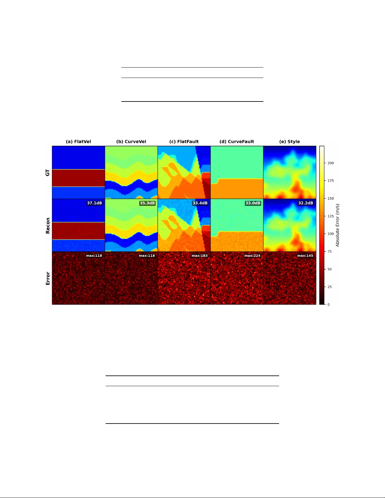
Comments & Academic Discussion
Loading comments...
Leave a Comment