Mixed difference integer-valued GARCH model for $ \mathbb{Z}$-valued time series

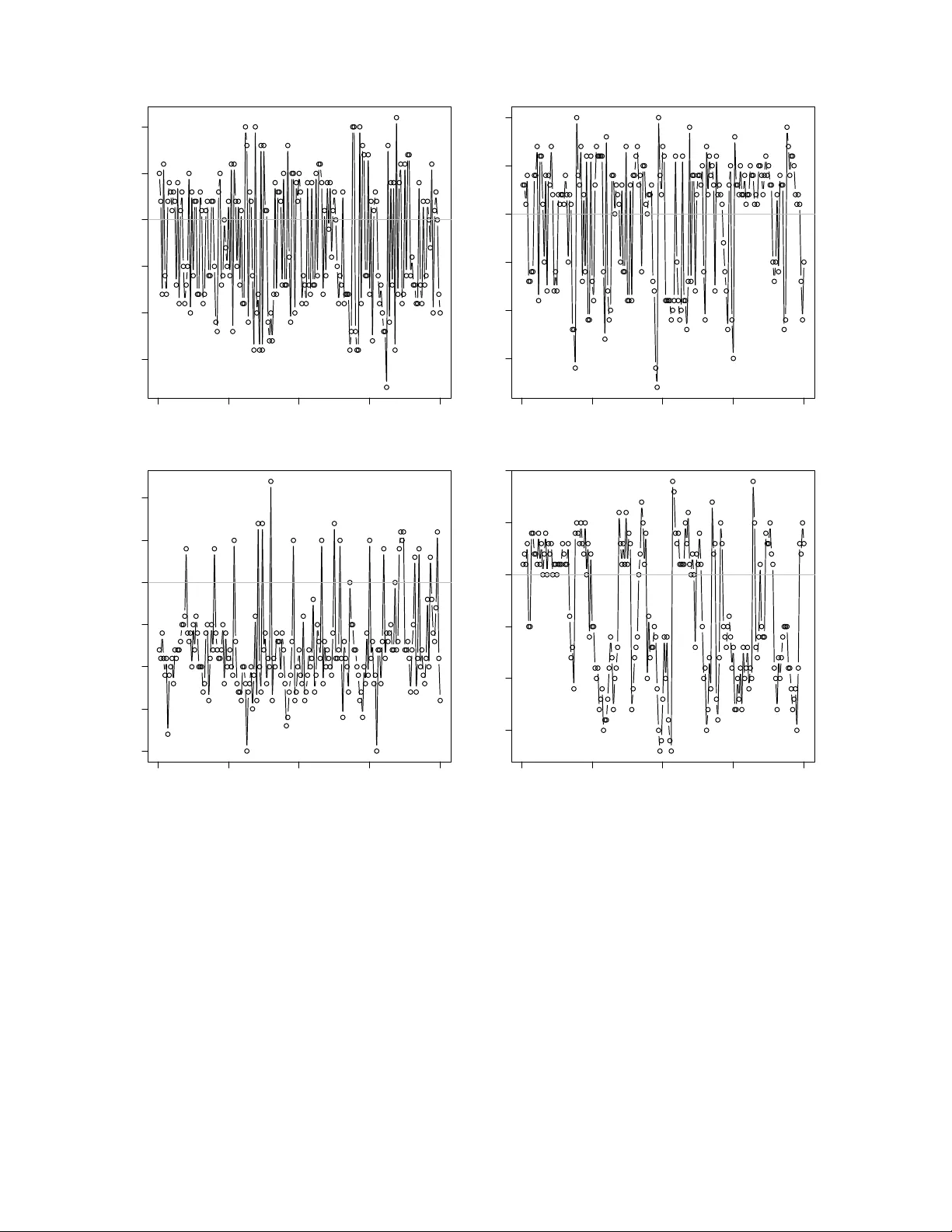
Mixed diﬀerence in teger-v alued GAR CH mo del for Z -v alued time series Ab delhakim Aknouc he ∗ , Christian F rancq † and Y uic hi Goto ‡ § Abstract In this pap er, w e in tro duce ﬂexible observ ation-driven Z -v alued time series models constructed from mixtures of negativ e and non-negative components. Compared to mo dels based on the standard Sk ellam distribution or on a diﬀerence of tw o integer- v alued v ariables, our sp eciﬁcation oﬀers greater v ersatility . F or example, it easily allo ws for sk ewness and bimo dalit y . F urthermore, the observ ation of one comp onen t of the mixture makes interpretation and statistical analysis easier. W e establish conditions for stationarity and mixing, and develop a mixed Poisson quasi-maximum lik eliho o d estimator with prov en asymptotic prop erties. A p ortman teau test is prop osed to di- agnose residual serial dep endence. The ﬁnite-sample performance of the metho dology is assessed via simulation, and an empirical application on tic k prices demonstrates its practical usefulness. JEL Classiﬁc ation: C22, C12 and C13 Keywor ds : Discrete diﬀerence distribution; GAR CH for tic k-by-tic k data, Mixed diﬀerence; Mixed Poisson QMLE; Random-weigh ting b o otstrap; Z -v alued time series. ∗ Qassim Univ ersity , e-mail: aknouche_ab@y aho o.com † CREST and Univ ersity of Lille, e-mail: christian.francq@ensae.fr ‡ Kyush u Universit y , e-mail: yuichi.goto@math.kyush u-u.ac.jp § The three authors con tributed equally to the pap er and are listed alphab etically 1 1 In tro duction Signed in teger-v alued ( Z -v alued) time series are common in applications suc h as ﬁnance (price changes), macro economics (interest rates in discrete steps), credit rating (agencies rate en tities on a discrete s cale), ecology (temp eratures), sp orts (score diﬀerences) and sometimes result from diﬀerenced coun t series. Existing modeling approac hes for Z -v alued time series fall into three categories. The ﬁrst category relies on sto c hastic models in v olving signed thinning operators, based on mo d- iﬁcations of the INAR model ( Kim and P ark , 2008 ; Kac hour and T ruquet , 2011 ; Alzaid and Omair , 2014 ) or in teger-v alued random co eﬃcient autoregressions ( Aknouc he et al. , 2025 ). Ho wev er, these models lead to complex likelihoo ds in volving intractable con volu- tions, making estimation more diﬃcult. The second approach is based on parameter-driven (or state-space) form ulations ( Rydb erg and Shephard , 2003 ; Liesenfeld et al. , 2006 ; Shahtah- massebi , 2011 ; Shahtahmassebi and Mo yeed , 2014 ; K o opman et al. , 2017 ; Barra and K o op- man , 2018 ). Although these form ulations are ﬂexible, laten t dynamics render the lik eliho o d in tricate, whic h mak es estimation computationally demanding and complicates prediction. The third approac h is based on observ ation-driv en GARCH-lik e representations, sp eciﬁcally , b y m ultiplying non-negativ e INGARCH mo dels b y a sign selector, which is an indep endent and iden tically distributed (i.i.d.) Bernoulli or i.i.d. three-p oint random v ariable that takes v alues in {− 1 , 0 , 1 } (see Hu and Andrews ( 2021 ); Xu and Zhu ( 2022 ); Li et al. ( 2024 )). The la ws of the innov ations of these time series mo dels are diﬀerence distributions, such as the standard Skellam distribution ( Irwin , 1937 ; Skellam , 1946 ) or the diﬀerence of tw o more general indep endent in teger-v alued v ariables. Unlike parameter-driv en mo dels, this approac h oﬀers mathematical tractability . In particular, the conditional likelihoo d is a v ailable, and prediction is straightforw ard. Therefore, this pap er focuses on this approach, but we adopt a ﬂexible semi-parametric approach and we relax the indep endence assumption on the tw o comp onen ts of the diﬀerence distribution (goals in a fo otball matc h are not independent) as w ell as the restrictiv e assumption of an independent sign selector. In this pap er, we prop ose a highly ﬂexible framework for Z -v alued time series: the dy- 2 namic Mixed Diﬀerence INGAR CH (MD-INGAR CH) model. Our approach generates a series as a mixed diﬀerence b et ween tw o non-negativ e components, with a Bernoulli selector determining which comp onen t is activ e at each time. The core inno v ation of our mo del is that the Bernoulli selector sequence itself can b e non-i.i.d. (e.g., follo wing its o wn IN- GAR CH pro cess). This crucial feature enables the conditional transition p robabilit y of the series’ sign to evolv e ov er time, a level of realism unattainable by existing mo dels based on an i.i.d. sign selector. F urthermore, unlik e usual existing mo dels that imply symmetry or unimo dality , our framework naturally accommo dates asymmetric and multimodal condi- tional distributions. Finally , we adopt a semi-parametric approac h. This means that w e do not assume that the conditional distributions of the tw o INGARCHs in the mixed diﬀerence are Poisson-distributed or follo w an y other sp eciﬁc distribution. Thanks to estimation b y a quasi-maxim um lik eliho o d approach in particular, our results remain v alid for a wide range of unsp eciﬁed conditional distributions. In ﬁnancial econometrics, mo deling high-frequency price changes is complicated by their discrete integer-v alued natu re and the well-documented asymmetry in volatilit y dynamics– often termed the “leverage eﬀect”. Existing mo dels either ignore the discreteness (con tin uous- v alued GAR CH mo dels) or impose restrictiv e independence assumptions on price mo vemen t directions and do not directly mo del the volatilit y 1 . W e address this issue by introducing a mo del that captures both magnitude dynamics and the state-dep enden t probability of price increases (i.e., tic k-b y-tick price v ariations), providing a uniﬁed framework for analyzing mark et microstructure and v olatilit y clustering. The pap er is organized as follows. Section 2 formally introduces the MD-INGARCH mo del, highlighting its adv an tages ov er existing approaches. Section 3 establishes conditions for the existence of stationary and ergodic solutions, and for the b eta-mixing prop erty . Section 4 prop oses a mixed P oisson quasi-maxim um likelihoo d estimator and shows its strong 1 Standard coun t time series models are called “INGAR CH” but this terminology is misleading b ecause, unlik e GAR CH models, these models are for the conditional mean rather than the conditional v ariance (whic h is determined b y the conditional distribution and the conditional mean) 3 consistency and asymptotic normality . A p ortmanteau test with b o otstrap impro vemen ts for mo del diagnostics is also dev elop ed. Finite-sample p erformance is in vestigated via sim ulation in Section 5 . The mo del’s practical utility is demonstrated through a real-data application in Section 6 . Section 7 concludes by fo cusing on applications in ﬁnancial econometrics. All pro ofs are collected in a supplemen tary ﬁle, and any reference to this ﬁle b egins with the letter ‘S’. 2 A mixed diﬀerence INGAR CH mo del In resp onse to the increased demand for mo deling dependent discrete pro cesses, the study of non-negative in teger-v alued time series has b ecome widespread. Popular mo dels include in teger-v alued autoregressive (INAR) mo dels (see for example McKenzie , 1985 ; Al-Osh and Alzaid , 1987 ) and integer-v alued generalised autoregressiv e conditional heteroscedasticit y (INGAR CH) mo dels (see for example F erland et al. , 2006 ). More recen tly , hierarchical mo dels hav e b een prop osed ( Catania and Di Mari , 2021 ), with further dev elopments detailed in Armillotta and F okianos ( 2023 ), Aknouche and F rancq ( 2023 ), Armillotta and Gorgi ( 2024 ), Goto and F ujimori ( 2025 ), among others. In this section, we introduce a new class of Z -v alued time series mo dels based on the concept of mixed diﬀerence. 2.1 Mo del Let F 1 λ and F 2 λ ∗ denote distribution functions supp orted on N 0 = { 0 , 1 , ... } and N = { 1 , 2 , ... } , resp ectiv ely , with means λ > 0 and λ ∗ > 1 , respectively . Let { B t , t ∈ Z } b e a { 0 , 1 } -v alued sequence. W e will deﬁne a Z -v alued process { Y t , t ∈ Z } whose sign is positive if { B t = 1 } and negative if { B t = 0 } . Let F t denote the sigma ﬁeld generated b y { Y u , u ≤ t } . Let π t = P ( B t = 1 | F t − 1 ) . The pro cess { Y t , t ∈ Z } is said to follo w a dynamic mixe d diﬀer enc e INGAR CH (MD-INGAR CH) model if for eac h t ∈ Z Y t = B t X 1 t − (1 − B t ) X 2 t , X st | F t − 1 ∼ F s λ st , s = 1 , 2 , (2.1) 4 where λ st = ω s + q X i =1 α si | Y t − i | + p X j =1 β sj λ s,t − j , s = 1 , 2 , (2.2) and ω 1 > 0 , α si ≥ 0 , β sj ≥ 0 . The condition ω 2 > 1 suﬃces to ensure λ 2 t > 1 a.s. for an y t . W e how ever impose the weak er condition 0 < 1 − P p j =1 β 2 j < ω 2 since λ 2 t = ω 2 + q X i =1 α 2 i | Y t − i | + p X j =1 β 2 j λ 2 ,t − j ≥ ω 2 + p X j =1 β 2 j λ 2 ,t − j , and then, denoting b y B the bac kshift op erator (1 − p X j =1 β 2 j B j ) λ 2 t ≥ ω 2 ⇒ λ 2 t ≥ ω 2 1 − P p j =1 β 2 j , whic h entails λ 2 t > 1 a.s. In the case p = q = 1 , we will use the simpliﬁed notation α s = α s 1 and β s = β s 1 . It is assumed that B t and X st ( s = 1 , 2 ) are conditionally indep endent given F t − 1 . The conditional mean and v ariance are then E ( Y t |F t − 1 ) = π t λ 1 t − (1 − π t ) λ 2 t , V ar ( Y t |F t − 1 ) = π t V ar ( X 1 t |F t − 1 ) + (1 − π t ) V ar ( X 2 t |F t − 1 ) + π t (1 − π t ) ( λ 1 t + λ 2 t ) 2 . Let us giv e some examples of F 1 λ , F 2 λ , and { B t } . Example 1 (Poisson MD-INGARCH model) . Prominent examples of F 1 λ and F 2 λ are the cdfs of the Poisson distribution P ( λ 1 t ) and the (right) shifted P oisson distribution S P ( λ 2 t ) , resp ectiv ely . The conditional distribution of Y t is given b y Y t |F t − 1 ∼ π t P ( λ 1 t ) + (1 − π t ) − S P ( λ 2 t ) , (2.3) where − S P ( λ ) stands for the cdf of a negative shifted P oisson v ariable Z := − X − 1 with mean − λ and probabilit y mass function (pmf ) f Z ( z ) = e − λ +1 ( λ − 1) − z − 1 ( − z − 1)! , z ∈ { ..., − 2 , − 1 } , X = − Z − 1 ∼ P ( λ − 1) being P oisson distributed with λ > 1 . 5 Example 2 (mixed Poisson MD-INGAR CH) . Other examples of F 1 λ and F 2 λ are, for giv en a mixing cumulativ e distribution function G on [0 , ∞ ) , the asso ciated mixed P oisson distri- bution deﬁned b y the masses p k = Z ∞ 0 ( λx ) k k ! e − λx dG ( x ) , k = 0 , 1 , . . . , and its shifted distribution, resp ectiv ely . P articularly , if we c ho ose G as a c.d.f. of Gamma distribution with shap e r and scale p/ (1 − p ) , the mixed P oisson distribution is a negative binomial distribution N B ( r , p ) , where r is the num b er of successes and p is the probabilit y of success on each trial. Mixed P oisson distributions are often used in insurance (see Willmot et al. , 2001 ) and hav e already b een used for coun t time series mo dels (see Christou and F okianos , 2015 ; Barreto-Souza and Simas , 2016 ). Example 3 (i.i.d. Bernoulli sequences) . Obvious example of { B t } is i.i.d. Bernoulli se- quences. Example 4 (Bernoulli INGARCH mo del) . An imp ortant example of { B t } is the Bernoulli INGAR CH (1 , 1) model P  B t = 1 | F B t − 1  = π t , π t = c + aB t − 1 + bπ t − 1 , t ∈ Z , (2.4) where F B t = σ { B t − u , u ≥ 0 } denotes the σ -algebra generated b y { B t − u , u ≥ 0 } and c, a and b are constants satisfying c > 0 , a ≥ 0 , b ≥ 0 with a + b + c < 1 (see, e.g., Diop and Kengne , 2017 ). Note that F B t − 1 ⊂ F t − 1 , and that B t and F t − 1 are conditionally independent given F B t − 1 in the sense that P ( B t = 1 | F t − 1 ) = P  B t = 1 | F B t − 1 , F t − 1  = P  B t = 1 | F B t − 1  . Since the Bernoulli distribution belongs to the one-parameter exp onential family , Theorems 3.1–3.2 in Aknouc he and F rancq ( 2021 ) ensure that { B t } is strictly stationary , ergo dic and b eta-mixing. Note that the INGARCH sequence { B t } is just i.i.d. when a = b = 0 with π t = c and reduces to a Marko v chain when b = 0 with π t = P ( B t = 1 | B t − 1 ) = c + aB t − 1 . 6 Remark 1 (Link with the threshold AR CH model) . The MD-INGAR CH model shares similarities with asymmetric GARCH mo dels, particularly the threshold ARCH (T ARCH) mo del prop osed b y Zak oian ( 1994 ) and expanded up on by Pan et al. ( 2008 ). The T AR CH mo del breaks down the symmetric eﬀect of p ositive and negative sho c ks on the curren t v olatility of the standard GAR CH mo del introduced b y Bollerslev ( 1986 ). F or simplicit y assume that B t follo ws a Bernoulli ARCH(1), i.e. b = 0 in ( 2.4 ). With an appropriate choice of the parameters, the MD-INGAR CH conditional mean E ( Y t | F t − 1 ) = λ 1 t π t − λ 2 t (1 − π t ) can b e (nearly) zero, as is the case for the T AR CH. Its v olatility can then b e measured b y E ( | Y t | | F t − 1 ) = cλ 1 t + (1 − c ) λ 2 t + B t − 1 a ( λ 1 t − λ 2 t ) . When applying the mo del to price increments, it is often observed that volatilit y increases more after a price drop ( i.e. B t − 1 = 0 ) than after an increase ( i.e. B t − 1 = 1 ) of the same magnitude. This stylized fact of ﬁnancial series can b e accounted for by setting λ 2 t > λ 1 t (see the empirical application of Section 6 ). An imp ortant diﬀerence with T AR CH mo dels, ho wev er, is that the MD-INGAR CH is applied to discretized data. This connection to the T ARCH mo del has imp ortant implications for ﬁnancial economet- rics. First, it allo ws us to quantify the asymmetric impact of past returns on future volatilit y in a setting where price changes are constrained to integer v alues—a common feature of tic k-by-tic k data that contin uous-v alued mo dels ignore. Second, b y mo deling E ( | Y t | | F t − 1 ) explicitly , w e can test h yp otheses ab out lev erage eﬀects (e.g., λ 2 t > λ 1 t ) using standard W ald or likelihoo d ratio tests. Third, the Bernoulli INGAR CH structure for π t pro vides a direct estimate of the time-v arying probability of a price increase, whic h is of indep endent interest in market microstructure research (e.g., predicting order ﬂo w im balance). Figure 1 illustrates time series plots generated from the follo wing Poisson MD-INGARCH mo del with a Bernoulli INGAR CH structure: Y t |F t − 1 ∼ π t P ( λ 1 t ) + (1 − π t ) − S P ( λ 2 t ) and B t |F B t − 1 ∼ Ber( π t ) where λ st = ω s + 0 . 3 | Y t − 1 | + 0 . 3 λ s,t − 1 for s = 1 , 2 and π t = c + aB t − 1 + bπ t − 1 7 with ω 1 = 1 and ω 2 = 4 . When a = b = 0 , B t reduces to a Bernoulli random v ariable with a constant success probabilit y c (Example 3 ). In this case, the sign transitions of the time series are random, as shown in the left panels. Conv ersely , the right panels depict the case of ( a, b )  = (0 , 0) (Example 4 ). In the b ottom-righ t panel, when B t − 1 = 1 (resp. 0 ), the conditional sign transition probabilit y is 0 . 9 (resp. 0 . 1 ), demonstrating a strong dep endence on past v alues. The top-right panel illustrates a more complex scenario where the transition probabilit y dep ends not only on B t − 1 but also on π t − 1 . Figure 2 displa ys pmfs for several densities. T op-left panel corresp onds to the pmf for the Sk ellam distribution with parameters λ 1 and λ 2 , reﬂecting the mo deling approach in Alomani et al. ( 2018 ) and Cui et al. ( 2021 ). F or λ 1 = λ 2 , the distribution is symmetric. When λ 1 < λ 2 , the distribution is righ t-skew ed, and when λ 1 > λ 2 , it is left-skew ed. The Sk ellam family is relativ ely simple and lac ks ﬂexibilit y in representing complex shap es. The other panels corresp ond to mixtures of non-negativ e and negative distributions, illustrating our proposed mo deling approac h. Speciﬁcally , we use P oisson and negative binomial distributions for non-negativ e v alues, and negativ ely shifted P oisson and negativ e binomial distrib utions for negativ e v alues, com bined with v arious mixing ratios. Our proposed mo deling framew ork oﬀers extensive ﬂexibilit y , enabling the represen tation of distributions with features suc h as sk ewness and bimo dality . 2.2 Mixed diﬀerence v ersus diﬀerence This section explains our c hoice of a mixture-based approac h ov er a direct diﬀerence ap- proac h. Let X 1 and X 2 b e tw o in teger-v alued random v ariables not necessarily indep endent and v alued in N 0 and N , respectively , with pmfs f X i ( · ) . Let also B a Bernoulli random v ariable indep endent of X 1 and X 2 with parameter π ∈ (0 , 1) . Deﬁne the Z -v alued random v ariable Y b y Y := B X 1 − (1 − B ) X 2 . Then, the pmf is given, for each z ∈ Z , b y f Y ( z ) = P ( Y = z ) = { π f X 1 ( z ) } 1 z ≥ 0 { (1 − π ) f X 2 ( − z ) } 1 z< 0 . (2.5) 8 0 50 100 150 200 −15 −10 −5 0 5 10 c=0.5, a=0, b=0 1:n X 0 50 100 150 200 −15 −10 −5 0 5 10 c=0.5, a=0.4, b=0.1 1:n X 0 50 100 150 200 −20 −15 −10 −5 0 5 10 c=0.1, a=0, b=0 1:n X 0 50 100 150 200 −15 −10 −5 0 5 10 c=0.1, a=0.8, b=0 1:n X Figure 1: Plots of time series generated b y the MD-INGARCH mo del with n = 200 . The left panels corresp ond to the case where ( a, b ) = (0 , 0) , indicating random transitions of the sign of the time series. The righ t panels corresp ond to the case where ( a, b )  = (0 , 0) , where the conditional transition probabilit y of the sign dep ends on past v alues, demonstrating more structured dynamics. 9 −10 −5 0 5 10 0.00 0.05 0.10 0.15 0.20 0.25 0.30 densities of Skellam(lambda1,lambda2) k density (lambda1,lambda2)=(1,1) (lambda1,lambda2)=(2,2) (lambda1,lambda2)=(3,3) (lambda1,lambda2)=(1,2) (lambda1,lambda2)=(1,3) (lambda1,lambda2)=(2,1) (lambda1,lambda2)=(3,1) −10 −5 0 5 10 0.00 0.05 0.10 0.15 0.20 densities of 0.6*P ois(lambda1)+0.4*shiftedNB(p,r2) with p=0.5 k density lambda1=1 lambda1=2 lambda1=3 lambda1=4 lambda1=5 r2=1 r2=2 r2=3 r2=3 r2=4 r2=5 −10 −5 0 5 10 0.00 0.05 0.10 0.15 densities of 0.5*P ois(lambda1) and 0.5*ShiftedP ois(lambda2) k density lambda1=1 lambda1=2 lambda1=3 lambda1=4 lambda1=5 lambda2=1 lambda2=2 lambda2=3 lambda2=4 lambda2=5 −10 −5 0 5 10 0.00 0.05 0.10 0.15 0.20 0.25 densities of 0.5*NB(p,r1) and 0.5*ShiftedNB(p,r2) with p=0.5 k density r1=1 r1=2 r1=3 r1=4 r1=5 r2=1 r2=2 r2=3 r2=4 r2=5 −10 −5 0 5 10 0.00 0.05 0.10 0.15 0.20 densities of 0.6*P ois(lambda1) and 0.4*shiftedP ois(lambda2) k density lambda1=1 lambda1=2 lambda1=3 lambda1=4 lambda1=5 lambda2=1 lambda2=2 lambda2=3 lambda2=4 lambda2=5 −10 −5 0 5 10 0.00 0.05 0.10 0.15 0.20 0.25 0.30 densities of 0.6*NB(p,r1) and 0.4*shiftedNB(p,r2) with p=0.5 k density r1=1 r1=2 r1=3 r1=4 r1=5 r2=1 r2=2 r2=3 r2=4 r2=5 Figure 2: Probability mass functions for v arious distributions. The top-left panel sho ws the Sk ellam distribution, corresp onding to the approac h in Alomani et al. ( 2018 ); Cui et al. ( 2021 ), while the other panels sho w mixtures of p ositive and negativ e distributions with diﬀeren t mixing ratios, corresponding to our approach. 10 In other w ords, Y ≥ 0 if and only if B = 1 (i.e. Y < 0 if and only if B = 0 ), so B is observ able (and indicates the sign of Y ). Thus Y is a mixture of X 1 and − X 2 , whic h we call “ mixe d diﬀer enc e ” b etw een X 1 and X 2 . The mixed diﬀerence can b e considered as an alternativ e to the standard diﬀerence X 1 − X 2 whic h sup erp oses X 1 and − X 2 . Compared to the con volution X 1 − X 2 , the mixed diﬀerence B X 1 − (1 − B ) X 2 has a muc h simpler distribution given by ( 2.5 ) without the need to assume the indep endence b etw een X 1 and X 2 . In particular, many distributions for X 1 and X 2 are allo wed, such as Poisson, negative binomial, generalized Poisson, and ev en b ounded-v alued discrete distributions suc h as Binomial and b eta-Binomial. Note that the fact that B is observ able when Y is observed greatly simpliﬁes the estimation of the distribution of B from data and thus the parameters of the distributions of X 1 and X 2 . F rom the deﬁnition of Y , X 1 and X 2 are not allo wed to b e equal b ecause they do not assume the same supp ort. This assumption is made to make the supp orts of X 1 and X 2 forming a partition of Z , which in turn will imply B observ able when Y is. Otherwise, that is, when X 1 and X 2 are b oth N 0 -v alued then B is not observ able when Y = 0 b ecause suc h a v alue can come from b oth X 1 and − X 2 . Note ﬁnally that Y = (2 B − 1) X has a symmetric distribution on Z when π = 0 . 5 . F or the abov e reasons, w e prop ose a mixture-based approac h instead of a sup erp osition of t wo opp osite discrete indep enden t random v ariables. 3 Prop erties of the MD-INGAR CH mo del This section presents the theoretical prop erties of the MD-INGARCH mo del. Let F λ b e a discrete cumulativ e distribution function (cdf ) with mean λ = R ∞ 0 xdF λ ( x ) . In Aknouche and F rancq ( 2021 ), F λ is said to satisfy a “sto c hastic-equal-mean order prop erty” if λ ≤ λ ∗ ⇒ F − λ ( u ) ≤ F − λ ∗ ( u ) , ∀ u ∈ (0 , 1) , (3.1) where F − λ is the generalized in v erse of F λ . Denote by F the class of suc h cdfs. Not only P oisson in Example 1 and mixed Poisson distributions in Example 2 satisfy ( 3.1 ), but also all mem b ers of the one-parameter exponential family (e.g., Poisson, negativ e binomial, ...), the 11 double Poisson, the negativ e binomial distribution with time-v arying n um b er of failures, the zero-inﬂated P oisson distribution, the zero-inﬂated negativ e binomial distribution, and mixed distributions of any distribution satisfying ( 3.1 ) enjoy the property ( 3.1 ). See Aknouche and F rancq ( 2021 ) for the details. In con trast to fully parametric Z -v alued time series mo dels—suc h as the INGAR CH mo del of Hu and Andrews ( 2021 ) and the GZG mo del of Xu and Zh u ( 2022 )—our approach is semi-parametric. W e model the conditional means λ st parametrically , but mak e only minimal assumptions ( i.e. F s λ ∈ F ) ab out the form of the conditional distributions. Assume there exist constan ts π + 1 ∈ (0 , 1) and π + 0 ∈ (1 − π + 1 , 1) suc h that π t ≤ π + 1 and 1 − π t ≤ π + 0 almost surely (a.s.). (3.2) Set r = max ( p, q ) and consider the matrix A ( l ) giv en b y A ( l ) =   α 1 l π + 1 + β 1 l α 1 l π + 0 α 2 l π + 1 α 2 l π + 0 + β 2 l   , 1 ≤ l ≤ r . Let A be deﬁned as A =            A (1) A (2) · · · A ( r − 1) A ( r ) I 2 0 2 × 2 · · · 0 2 × 2 0 2 × 2 0 2 × 2 I 2 · · · 0 2 × 2 0 2 × 2 . . . . . . . . . . . . . . . 0 2 × 2 0 2 × 2 · · · I 2 0 2 × 2            and denote by ρ ( A ) the spectral radius of A , i.e., the maxim um absolute eigen v alues of A . 3.1 Stationarit y conditions The follo wing result giv es a suﬃcien t condition for the existence of a stationary and ergo dic solution to the MD-INGAR CH mo del. Prop osition 3.1. Assume that F 1 λ and F 2 λ satisfy ( 3.1 ) and have r esp e ctive supp orts N 0 = { 0 , 1 , ... } and N = { 1 , 2 , ... } . Assume that { B t , t ∈ Z } is stationary and er go dic with ( 3.2 ) . 12 Ther e exists a stationary and er go dic pr o c ess { Y t } satisfying ( 2.1 ) - ( 2.2 ) if ρ ( A ) < 1 . (3.3) This solution satisﬁes E | Y t | < ∞ and E λ st < ∞ for s = 1 , 2 . (3.4) If ther e exists a stationary pr o c ess { Y t } satisfying ( 2.1 ) - ( 2.2 ) and ( 3.4 ) then p X j =1 β sj < 1 for s = 1 , 2 . (3.5) Ob viously , the suﬃcien t stationarity condition ( 3.3 ) implies the necessary stationarity condition ( 3.5 ), but the former is generally muc h more restrictive. The follo wing proposition sho ws that this suﬃcien t condition is optimal in the case of Example 3 . Prop osition 3.2. If { B t } is i.i.d. (Example 3 ), with P ( B t = 1) = π ∈ (0 , 1) , then Pr op osi- tion 3.1 holds with A ( l ) =   α 1 l π + β 1 l α 1 l (1 − π ) α 2 l π α 2 l (1 − π ) + β 2 l   , 1 ≤ l ≤ r. Mor e over, the c ondition ( 3.3 ) is ne c essary and suﬃcient for the existenc e of a stationary solution such that E λ st < ∞ for s = 1 , 2 . If { B t } is a Marko v c hain, with transition probabilities p ( i, j ) = P ( B t = j | B t − 1 = i ) ∈ (0 , 1) for i, j ∈ { 0 , 1 } , then Prop osition 3.1 holds with π + 1 = max { p (0 , 1) , p (1 , 1) } and π + 0 = max { p (1 , 0) , p (0 , 0) } . F or the Bernoulli INGARCH mo del (Example 4 ), Prop osition 3.1 holds with π + 1 = a + b + c and π + 0 = 1 − c . A necessary condition, sharper than ( 3.5 ), for the existence of a stationary solution with a ﬁnite mean is given b y the following result. Prop osition 3.3. Consider the c ase wher e { B t } is an i.i.d. Bernoul li se quenc e with p ar am- eter π ∈ (0 , 1) . If ther e exists a stationary pr o c ess { Y t } satisfying ( 2.1 ) - ( 2.2 ) and ( 3.4 ) then 13 ( 3.5 ) and π 1 − p X j =1 β 1 j ! − 1 q X i =1 α 1 i + (1 − π ) 1 − p X j =1 β 2 j ! − 1 q X i =1 α 2 i < 1 (3.6) hold. Under the conditions of the previous prop osition, w e ha ve E | Y t | =     1 − π q P i =1 α 1 i 1 − p P j =1 β 1 j − (1 − π ) q P i =1 α 2 i 1 − p P j =1 β 2 j     − 1     π ω 1 1 − p P j =1 β 1 j + (1 − π ) ω 2 1 − p P j =1 β 2 j     . F or example, when p = q = 1 , the means of Y t and | Y t | are giv en b y E ( | Y t | ) = π ω 1 (1 − β 2 ) + (1 − π ) ω 2 (1 − β 1 ) (1 − β 1 )(1 − β 2 ) − π α 1 (1 − β 2 ) − (1 − π ) α 2 (1 − β 1 ) , E ( Y t ) = π ω 1 + α 1 E ( | Y t | ) 1 − β 1 − (1 − π )  ω 2 + α 2 E ( | Y t | ) 1 − β 2  . The next prop osition shows that the explicit necessary conditions ( 3.5 ) and ( 3.6 ) can be necessary and suﬃcien t. Prop osition 3.4. Consider a pr o c ess { Y t } satisfying ( 2.1 ) – ( 2.2 ) and ( 3.4 ) . Supp ose p = q = 1 and { B t } is an i.i.d. Bernoul li se quenc e with p ar ameter π ∈ (0 , 1) . Then, the c onditions ( 3.5 ) and ( 3.6 ) ar e e quivalent to ( 3.3 ) . 3.2 Mixing conditions F or a real pro cess { X t , t ∈ Z } and −∞ ≤ t ≤ s ≤ ∞ we use the notation X t : s = ( X t , X t +1 , . . . , X s ) and X s : t = ( X s , X s − 1 , . . . , X t ) . Let { Y t , t ∈ Z } b e the stationary pro- cess deﬁned in the proof of Prop osition 3.1 . Denote b y B the Borel sigma-algebra of R ∞ . F or h ≥ 0 , let the β -mixing co eﬃcien t β Y ( h ) = E sup A ∈B | P ( Y t + h : ∞ ∈ A | Y −∞ : t ) − P ( Y t + h : ∞ ∈ A ) | . W e can think of β Y ( h ) as a kind of measure of the dep endence b et ween the past and future of the pro cess { Y t , t ∈ Z } , if the past and future are separated by h dates (see Bradley ( 2005 ) for 14 a survey on mixing). The geometric decrease of the β -mixing co eﬃcients sho wn in the next prop osition is a desirable probabilistic prop ert y which, for instance, en tails the existence of a cen tral limit theorem on general transformations of the pro cess (see e.g. Herrndorf , 1984 ). Prop osition 3.5. Supp ose { B t } fol lows the Bernoul li INGARCH (1 , 1) mo del of Example 4 and the other assumptions of Pr op osition 3.1 , in p articular ( 3.3 ) , ar e satisﬁe d. Ther e exists a stationary and er go dic MD-INGAR CH pr o c ess { Y t , t ∈ Z } satisfying ( 2.1 ) - ( 2.2 ) , and ther e exist c onstants K > 0 and ϱ ∈ (0 , 1) such that β Y ( h ) ≤ K ϱ h , h ≥ 0 . 4 Inference Let Y 1 , Y 2 , ..., Y n b e a ﬁnite sample-path generated from model ( 2.1 ) and B 1 , B 2 , ..., B n b e the corresp onding observ ation-sign indicators. Assume that the generating pro cess { B t } has the Bernoulli INGAR CH (1 , 1) representation of Example 4 . Our ﬁrst aim is to estimate the true parameter θ 0 =  ϕ ⊤ 0 , ψ ⊤ 0  ⊤ ∈ Θ := Φ × Ψ where ϕ 0 = ( a 0 , b 0 , c 0 ) ⊤ ∈ Φ ⊂ (0 , 1) × [0 , 1) 2 and ψ ⊤ 0 =  ψ ⊤ 01 , ψ ⊤ 02  ∈ Ψ = Ψ 1 × Ψ 2 with ψ 0 s = ( ω 0 s , α 0 s 1 , ..., α 0 sq , β 0 s 1 , ..., β 0 sp ) ⊤ ∈ Ψ s ⊂ (0 , ∞ ) × [0 , ∞ ) q + p for s = 1 , 2 . Since we do not w ant to make strong parametric assumptions on the conditional distributions F 1 λ and F 2 λ , we prop ose a semi-parametric estimator, more precisely , the mixed Poisson maxim um quasi-lik eliho o d (MP-QML) estimator. W riting in ( 2.2 ) the true intensities λ st := λ st ( ψ 0 s ) in terms of the true parameter ψ 0 s , let λ st ( ψ s ) ( s = 1 , 2 ) b e the generic in tensit y function deﬁned for any generic parameter ψ :=  ψ ⊤ 1 , ψ ⊤ 2  ⊤ ∈ Ψ and all t ∈ Z by λ st ( ψ s ) = ω s + q X i =1 α si | Y t − i | + p X j =1 β sj λ s,t − j ( ψ s ) , s = 1 , 2 , (4.1) where ψ s = ( ω s , α s 1 , ..., α sq , β s 1 , ..., β sp ) ⊤ . The sequence { λ st ( ψ s ) , t ∈ Z } uniformly exists almost surely whenev er p X j =1 β sj < 1 , s = 1 , 2 (4.2) 15 for every ψ s ∈ Ψ s . Since the β sj ’s are p ositiv e, by Corollary 2.2 in F rancq and Zakoian ( 2019 ), when the Ψ s ’s are compact, ( 4.2 ) is equiv alent to max ψ s ∈ Ψ s ρ ( B s ) < 1 , s = 1 , 2 (4.3) where B s :=         β s 1 β s 2 · · · β sp 1 0 · · · 0 . . . . . . . . . . . . 0 · · · 1 0         . As λ st ( ψ s ) is not computable from a ﬁnite dataset, let e λ 10 , ..., e λ 1 , 1 − p , e λ 20 , ..., e λ 2 , 1 − p , Y 0 , ..., Y 1 − q b e ﬁxed starting v alues and deﬁne e λ st ( ψ s ) to b e a data-computable coun ter- part of λ st ( θ ) giv en by e λ st ( ψ s ) = ω s + q X i =1 α si | Y t − i | + p X j =1 β sj e λ s,t − j ( ψ s ) , t ≥ 1 . Similarly , for an y ϕ ∈ Φ , let π t ( ϕ ) b e the probability parameter function giv en by π t ( ϕ ) = c + aB t − 1 + bπ t − 1 ( ϕ ) , t ∈ Z (4.4) and let e π t ( ϕ ) b e an observ able proxy of π t ( ϕ ) given b y e π t ( ϕ ) = c + aB t − 1 + b e π t − 1 ( ϕ ) , t ≥ 1 , for some arbitrary ﬁxed initial v alues for B 0 and e π 0 . Note that ( 4.4 ) is well-deﬁned since b ∈ [0 , 1) . It will b e seen that under ( 4.2 ), the choice of initial v alues e λ 10 , ..., e λ 1 , 1 − p , e λ 20 , ..., e λ 2 , 1 − p , Y 0 , ..., Y 1 − q , B 0 , e π 0 is unimp ortant asymptotically . 4.1 Mixed P oisson QMLE Mo del ( 2.1 ) en tails f Y t |F t − 1 ( y ) = ( π t f X 1 t ( y )) 1 y ≥ 0 ((1 − π t ) f − X 2 t ( y )) 1 y< 0 16 where f Y t |F t − 1 ( y ) = P ( Y t = y | F t − 1 ) denotes the conditional pmf. If X 1 t w ere Poisson distributed with mean λ 1 t , and X 2 t w ere shifted Poisson distributed with mean λ 2 t (i.e. X 2 t = Z t + 1 with Z t ∼ P ( λ 2 t − 1) ), then the log-conditional pmf of Y t w ould b e given b y log( f Y t |F t − 1 ( y )) = (log ( π t ) − λ 1 t + y log ( λ 1 t ) − log ( y !)) 1 y ≥ 0 + (log (1 − π t ) − λ 2 t + 1 − ( y + 1) log ( λ 2 t − 1) − log(( − y − 1)!)) 1 y < 0 . Th us, w e prop ose to estimate the true parameter θ 0 using the mixed P oisson QMLE (MP-QMLE), which is a measurable solution to the following problem b θ n = arg max θ ∈ Θ e L n ( θ ) with e L n ( θ ) = 1 n n X t =1 e ℓ t ( θ ) (4.5) where e ℓ t ( θ ) =  log ( e π t ( ϕ )) − e λ 1 t ( ψ 1 ) + Y t log( e λ 1 t ( ψ 1 ))  1 Y t ≥ 0 +  log (1 − e π t ( ϕ )) − e λ 2 t ( ψ 2 ) − ( Y t + 1) log ( e λ 2 t ( ψ 2 ) − 1)  1 Y t < 0 . (4.6) T o study the consistency and asymptotic normalit y of the MP-QMLE giv en by ( 4.5 ) w e consider the follo wing assumptions. Assumption 1. A1. Conditions of Prop osition 3.1 (at θ 0 ) and ( 4.2 ) (or equiv alently ( 4.3 )) are satisﬁed. A2. W e ha v e E ( X τ st ) < ∞ for some τ > 1 , s = 1 , 2 . A3(i). The polynomials α 0 s ( z ) = q P i =1 α 0 si z i and β 0 s ( z ) = 1 − p P j =1 β 0 sj z j ha ve no common ro ot, α 0 s (1)  = 0 , and α 0 sq + β 0 sp  = 0 , s = 1 , 2 . A3(ii). The co eﬃcien t a 0  = 0 . A4. The parameter space Θ is compact and θ 0 ∈ Θ . A5. The true parameter θ 0 is in the in terior of Θ . A6. F or s = 1 , 2 and some ε > 0 w e ha ve E  V ar( X st |F t − 1 ) λ st ( ψ 0 s )  1+ ε < ∞ . 17 These assumptions are standard and resem ble those giv en for similar QMLEs of in teger- v alued mo dels. See e.g. Ahmad and F rancq ( 2016 ) for the P oisson QMLE. In particular A3(i) - A3(ii) are identiﬁabilit y conditions. If A3(ii) w ould not hold we could write π t = c 0 = c 0 (1 − b ) + bπ t − 1 under man y forms. Let D → n →∞ and a.s. → n →∞ denote, resp ectively , the con vergence in distribution and almost sure con v ergence as n → ∞ . W e will show the existence and in vertibilit y of Π = E  1 π t ( ϕ 0 ) (1 − π t ( ϕ 0 )) ∂ π t ( ϕ 0 ) ∂ ϕ ∂ π t ( ϕ 0 ) ∂ ϕ ⊤  J 1 = E  Y t λ 2 1 t ( ψ 01 ) ∂ λ 1 t ( ψ 01 ) ∂ ψ 1 ∂ λ 1 t ( ψ 01 ) ∂ ψ ⊤ 1 1 [ Y t ≥ 0]  , I 1 = E   Y t − λ 1 t ( ψ 01 ) λ 1 t ( ψ 01 )  2 ∂ λ 1 t ( ψ 01 ) ∂ ψ 1 ∂ λ 1 t ( ψ 01 ) ∂ ψ ⊤ 1 1 [ Y t ≥ 0]  J 2 = E  Y t +1 ( λ 2 t ( ψ 02 ) − 1) 2 ∂ λ 2 t ( ψ 02 ) ∂ ψ 2 ∂ λ 2 t ( ψ 02 ) ∂ ψ ⊤ 2 1 [ Y t < 0]  , I 2 = E   Y t + λ 2 t ( ψ 02 ) λ 2 t ( ψ 02 ) − 1  2 ∂ λ 2 t ( ψ 02 ) ∂ ψ 2 ∂ λ 2 t ( ψ 02 ) ∂ ψ ⊤ 2 1 [ Y t < 0]  , where σ 2 st = V ar ( X st | F t − 1 ) . Let the blo c k-diagonal matrices J = diag ( Π , J 1 , J 2 ) , Σ = diag  Π − 1 , J − 1 1 I 1 J − 1 1 , J − 1 2 I 2 J − 1 2  . Theorem 4.1. i) Under A1 - A4 , b θ n a.s. → n →∞ θ 0 . (4.7) ii) If, in addition, A5 - A6 hold, then √ n  b θ n − θ 0  = J − 1 1 √ n n X t =1 ∆ t ξ t + o P (1) D → n →∞ N (0 , Σ ) , (4.8) where ∆ t = diag  1 π t (1 − π t ) ∂ π t ∂ ϕ , 1 λ 1 t ∂ λ 1 t ∂ ψ 1 , 1 λ 2 t − 1 ∂ λ 2 t ∂ ψ 2  ∈ F t − 1 and ξ ⊤ t = { B t − π t , B t ( X 1 t − λ 1 t ) , (1 − B t )( X 2 t − λ 2 t ) } such that { ξ t , F t } is a martingale diﬀerence sequence. T o apply ( 4.8 ), an estimator of Σ is required. The matrix Π can b e estimated empirically b y b Π := 1 n n X t =1 1 e π t  b ϕ n   1 − e π t  b ϕ n  ∂ e π t  b ϕ n  ∂ ϕ ∂ e π t  b ϕ n  ∂ ϕ ⊤ . 18 Similar empirical estimators b J 1 , b I 1 , b J 2 and b I 2 are deﬁned. W e then set b J = diag ( b Π , b J 1 , b J 2 ) and b Σ = diag  b Π − 1 , b J − 1 1 b I 1 b J − 1 1 , b J − 1 2 b I 2 b J − 1 2  when the matrix b J is inv ertible, whic h holds true almost surely when n is large enough. Remark 2. When X 1 t is P oisson distributed and X 2 t is shifted Poisson distributed, we hav e V ar ( X 1 t |F t − 1 ) = λ 1 t ( ψ 01 ) and V ar ( X 2 t |F t − 1 ) = λ 2 t ( ψ 01 ) − 1 . Hence the equalities I 1 = J 1 and I 2 = J 2 hold so Σ simpliﬁes to diag  Π − 1 , J − 1 1 , J − 1 2  , which is the inv erse of the Fisher information matrix. Thus, in this case, the MP-QMLE is asymptotically eﬃcien t. Remark 3. Note that the ﬁrst-order conditions of the optimization problem ( 4.5 )-( 4.6 ) deﬁne b ϕ n , b ψ 2 n and b ψ 1 n indep enden tly . Therefore b θ n is deﬁned b y b ϕ n = arg max ϕ ∈ Φ 1 n n X t =1 log ( e π t ( ϕ )) 1 Y t ≥ 0 + log (1 − e π t ( ϕ )) 1 Y t < 0 b ψ 1 n = arg max ψ 1 ∈ Ψ 1 1 n n X t =1  − e λ 1 t ( ψ 1 ) + Y t log( e λ 1 t ( ψ 1 ))  1 Y t ≥ 0 b ψ 2 n = arg max ψ 2 ∈ Ψ 2 1 n n X t =1  − e λ 2 t ( ψ 2 ) − ( Y t + 1) log ( e λ 2 t ( ψ 2 ) − 1))  1 Y t < 0 . Since the latter estimates are computationally muc h easier than ( 4.5 )-( 4.6 ), we will adopt them in applications. Note that the block-diagonal form of Σ is consistent with the fact that b θ n is obtained b y computing three separate MP-QMLEs. 4.2 Go o dness-of-ﬁt tests In this section, w e present a p ortman teau test to ev aluate the suitability of MD-INGAR CH mo dels. These tests examine whether the ﬁrst residual auto correlations (up to a certain lag) are join tly signiﬁcant. Portman teau tests are among the most popular diagnostic tools in time series analysis. F or a reference b o ok dev oted to this class of tests, see Li ( 2003 ). F or more recen t sources, see Boubacar Mainassara et al. ( 2022 ) and the references therein. F or a Portman teau test for in teger-v alued time series, see also Ahmad ( 2016 ). 19 The residuals of the MD-INGARCH mo del are b ϵ 1 , . . . , b ϵ n , where b ϵ t = e ϵ t ( b θ n ) with e ϵ t ( θ ) := Y t − I { Y t ≥ 0 } e λ 1 t ( ψ 1 ) + I { Y t < 0 } e λ 2 t ( ψ 2 ) , 1 ≤ t ≤ n, and the con ven tion e ϵ t ( · ) ≡ 0 when t < 1 or t > n . Let ϵ t ( θ ) = Y t − I { Y t ≥ 0 } λ 1 t ( ψ 1 ) + I { Y t < 0 } λ 2 t ( ψ 2 ) and ϵ t = ϵ t ( θ 0 ) . Under the assumption of Theorem 4.1 , { ϵ t } is uncorrelated: for h > 0 w e ha v e E ( ϵ t − h ϵ t ) = E { ϵ t − h E ( ϵ t | F t − 1 ) } = 0 . The empirical residual auto correlation at lag h is deﬁned b y b ρ h = b γ h b γ 0 , b γ h = 1 n n X t =1 b ϵ t b ϵ t − h . The idea b ehind the go o dness-of-ﬁt p ortmanteau test is that, if the mo del is correctly sp ec- iﬁed and the other assumptions of Theorem 4.1 hold, then the residuals should b e close to the innov ations, and thus the b ρ h ’s should all be close to zero. F or some ﬁxed in teger k > 0 , let the vector b ρ 1: k = ( b ρ 1 , . . . , b ρ k ) ⊤ . W e are going to sho w that, under the assumptions of Theorem 4.1 , √ n b ρ 1: k D → n →∞ N ( 0 , V 0 ) for some in vertible matrix V 0 . T o deﬁne V 0 w e need to in tro duce the follo wing matrices. Let E be the k × k matrix with generic elemen t E ( i, j ) = E ϵ 2 t ϵ t − i ϵ t − j . Let D be the k × d matrix whose line i is D ( i, · ) = E ϵ t ∂ ∂ θ ⊤ ϵ t + i ( θ 0 ) , where d = 2( p + q ) + 3 is the dimension of θ . Let C b e the k × d matrix whose line i is C ( i, · ) = E ϵ t ϵ t − i ∂ ∂ θ ⊤ ℓ t ( θ 0 ) . W e also need the d × d matrix J = diag ( Π , J 1 , J 2 ) . In the next theorem, we will show that V 0 = 1 ( E ϵ 2 t ) 2  E + C J − 1 D ⊤ + D J − 1 C ⊤ + D Σ D ⊤  . Let the empirical estimators b E := 1 n n X t =1 b ϵ 2 t b ϵ t − i b ϵ t − j ! 1 ≤ i,j ≤ k , b D := 1 n n X t =1 b ϵ t ∂ ∂ θ j b ϵ t + i ! 1 ≤ i ≤ k, 1 ≤ j ≤ d , b E ϵ 2 t := 1 n n X t =1 b ϵ 2 t , b C := 1 n n X t =1 b ϵ t b ϵ t − i ∂ ∂ θ j e ℓ t ( b θ n ) ! 1 ≤ i ≤ k, 1 ≤ j ≤ d , and let b V b e the empirical estimator of V 0 obtained by plugging. W e generally ha ve b ρ 1: k a.s. → n →∞ ρ 1: k and b V a.s. → n →∞ V (4.9) 20 with ρ 1: k = 0 k and V = V 0 when the mo del is correctly sp eciﬁed, and p ossibly with ρ 1: k  = 0 k when the model is missp eciﬁed. Let χ 2 k ( α ) b e the α -quan tile of the chi-squared distribution with k degrees of freedom. F or the existence of the matrices D and E , we need the following momen t condition. A7. F or s = 1 , 2 w e hav e E X 4 st < ∞ . W e also need the follo wing identiﬁabilit y condition. A8. With probability one, the random v ariable X 1 t − λ 1 t + X 2 t − λ 2 t is not zero. The previous assumption is v ery mild, but necessary in order to rule out pathological distri- butions, as illustrated b y the follo wing example. Remark 4 (An example sho wing that A8 is not v acuous) . Assume that X 1 t = X 2 t = c for some constan t c ∈ N suc h that (for some particular v alues of ω , α and β ) λ st ≡ c = ω + αc + β c , then A8 is not satisﬁed. Theorem 4.2. Supp ose π t follo ws the Bernoulli INGARCH(1,1) mo del of Example 4 . Under A1 - A8 , we ha ve the null H 0 : ( 4.9 ) holds with ρ 1: k = 0 k and V = V 0 is non-singular, and the test of rejection region C = { n b ρ ⊤ 1: k b V − 1 b ρ 1: k > χ 2 k (1 − α ) } has the asymptotic lev el α ∈ (0 , 1) . Under the alternative H 1 : ( 4.9 ) holds with ρ 1: k  = 0 k , if V is in vertible, the test of rejection region C is consisten t. T o better con trol ﬁrst-kind error, w e apply the random-w eighting (R W) b o otstrapping metho d (see Zh u ( 2016 ) and its references). Let a sequence of p ositiv e i.i.d. random v ariables { w ∗ t } , indep endent of the data sequence { Y t } , with b oth mean and v ariance one. Step 1 of Zh u’s R W metho d consists of computing a b o otstrapp ed estimator of θ 0 through the n umerical optimization of an R W ob jective function. T o reduce the computational burden of this ﬁrst step, we used the tric k prop osed by Kreiss et al. ( 2011 ) and Shimizu ( 2013 ) and 21 deﬁne b θ ∗ n = b θ n + b J − 1 1 n n X t =1 ( w ∗ t − 1) ∂ ∂ θ e ℓ t  b θ n  . This tric k sa ves time b y using a Newton-Raphson type iteration instead of a full n umerical optimization to compute the b o otstrap estimator. W e then pro ceed to Step 2 of Zh u’s R W metho d and compute the bo otstrapp ed quantities b ρ ∗ 1: k =      e ρ ∗ 1  b θ ∗ n  . . . e ρ ∗ k  b θ ∗ n       − b ρ 1: k , where e ρ ∗ h ( · ) = e γ ∗ h ( · ) b γ 0 and e γ ∗ h ( θ ) = 1 n n X t =1 w ∗ t e ϵ t ( θ ) e ϵ t − h ( θ ) . Theorem 4.3. Supp ose π t follo ws the Bernoulli INGAR CH(1,1) mo del of Example 4 . Con- ditional on almost all realization of { Y t } , under A1 - A8 , √ n b ρ ∗ 1: k con verges in distribution to the centered Gaussian distribution with v ariance V as n → ∞ . Let b ρ ∗ (1) 1: k , . . . , b ρ ∗ ( B ) 1: k b e B indep endent replications of b ρ ∗ 1: k , and let b V ∗ n their empirical v ariance. In view of the previous theorem, it is natural to consider the tests based on the follo wing p-v alues p 1 ,n := 1 − Ψ k  n b ρ ⊤ 1: k b V ∗− 1 n b ρ 1: k  and p 2 ,n := 1 B B X j =1 1 n b ρ ∗ ( j ) ⊤ 1: k b ρ ∗ ( j ) 1: k > b ρ ⊤ 1: k b ρ 1: k o , where Ψ k ( · ) denotes the cum ulative distribution function of the c hi-square distribution with k degrees of freedom. W e reject H 0 whenev er p j,n < 0 . 05 . Based on the Mon te Carlo exp erimen ts w e conducted, it seems that B = 500 replications are suﬃcien t and that the metho d is not v ery sensitive to the distribution of ω ∗ t , so that the standard exp onential distribution used in Zh u ( 2016 ) is appropriate. 22 5 Numerical study In this section, we conduct numerica l simulations to ev aluate the ﬁnite-sample performance of the proposed metho d. 5.1 P arameter estimation First, w e ev aluate the ﬁnite-sample performance of the mixed P oisson QMLE. The pro ce- dure is as follows: F or eac h time series length n ∈ { 1800 , 3600 , 7200 } , we generate 1000 indep enden t tra jectories from the MD-INGAR CH model Y t |F t − 1 ∼ π t P ( λ 1 t ) + (1 − π t ) − S P ( λ 2 t ) (5.1) or Y t |F t − 1 ∼ π t N B  p, pλ 1 t (1 − p )  + (1 − π t ) − S N B  p, pλ 2 t (1 − p )  (5.2) with a Bernoulli INGAR CH structure B t |F B t − 1 ∼ Ber( π t ) , where λ st = ω s + 0 . 3 | Y t − 1 | + 0 . 3 λ s,t − 1 for s = 1 , 2 and π t = 0 . 2 + 0 . 2 B t − 1 + 0 . 2 π t − 1 with p = 0 . 5 , ω 1 = 1 , and ω 2 = 2 . Then, w e compute the mixed Poisson (Q)MLE. Based on the estimators’ asymptotic distribution, w e also obtain appro ximations of their standard deviations. Figure 3 reports boxplots of the bias (estimator minus true v alue) for eac h parameter. F or eac h sample size, the lab els P ois and NB corresp ond to the cases where the data are generated from the mixed P oisson and mixed negative binomial mo dels, resp ectively , while estimation is carried out b y the mixed P oisson (Q)MLE in b oth cases. The estimation biases for all parameters are close to zero, and the disp ersion of the estimates decreases as the sample size n increases. As exp ected, the v ariability is generally larger when the data are generated from the mixed negative binomial mo del than from the mixed P oisson mo del. 23 −0.10 −0.05 0.00 0.05 0.10 c Bias (estimator − true) Pois n=1800 NB n=1800 Pois n=3600 NB n=3600 Pois n=7200 NB n=7200 −0.05 0.00 0.05 a Bias (estimator − true) Pois n=1800 NB n=1800 Pois n=3600 NB n=3600 Pois n=7200 NB n=7200 −0.4 −0.2 0.0 0.2 0.4 b Bias (estimator − true) Pois n=1800 NB n=1800 Pois n=3600 NB n=3600 Pois n=7200 NB n=7200 −1.0 −0.5 0.0 0.5 1.0 omega1 Bias (estimator − true) Pois n=1800 NB n=1800 Pois n=3600 NB n=3600 Pois n=7200 NB n=7200 −0.10 −0.05 0.00 0.05 0.10 alpha1 Bias (estimator − true) Pois n=1800 NB n=1800 Pois n=3600 NB n=3600 Pois n=7200 NB n=7200 −0.3 −0.2 −0.1 0.0 0.1 0.2 0.3 beta1 Bias (estimator − true) Pois n=1800 NB n=1800 Pois n=3600 NB n=3600 Pois n=7200 NB n=7200 −1.0 −0.5 0.0 0.5 1.0 omega2 Bias (estimator − true) Pois n=1800 NB n=1800 Pois n=3600 NB n=3600 Pois n=7200 NB n=7200 −0.10 −0.05 0.00 0.05 0.10 alpha2 Bias (estimator − true) Pois n=1800 NB n=1800 Pois n=3600 NB n=3600 Pois n=7200 NB n=7200 −0.3 −0.2 −0.1 0.0 0.1 0.2 0.3 beta2 Bias (estimator − true) Pois n=1800 NB n=1800 Pois n=3600 NB n=3600 Pois n=7200 NB n=7200 Figure 3: Boxplots of the bias (estimator minus true v alue) for each parameter based on 1000 replications. F or each parameter, the six b oxplots correspond to n = 1800 , 3600 , 7200 under data generated from the mixed Poisson mo del (P ois) and the mixed negative binomial mo del (NB). In all cases, estimation is carried out by mixed Poisson (Q)MLE. 24 Figure 4 presents a comparison b etw een the asymptotic standard errors and the empirical standard deviations of the mixed Poisson QMLE. The boxplots summarize the estimated standard deviations obtained from the asymptotic v ariance expressions, and the solid lines represen t the empirical standard deviations computed ov er replications. The v ariances under data generated from the mixed P oisson mo dels are smaller than those under data generated from the mixed NB mo dels. As the sample size increases, the v ariances decrease. Moreov er, in most cases, the empirical standard deviations lie within the corresp onding b oxplots of the estimated standard errors, indicating that the asymptotic v ariance form ulas pro vide reasonable appro ximations in ﬁnite samples. Finally , the v ariance estimators of c , ω 1 , and ω 2 tend to exhibit an upw ard bias. Conv ersely , the estimators of b , β 1 , and β 2 exhibit a do wnw ard bias. 5.2 P ortman teau test Second, we ev aluate the p erformance of the random w eight-based p ortmanteau test. W e generate time series of length n ∈ { 300 , 600 , 900 } from diﬀeren t mo dels under the n ull and alternativ e hypotheses. Under the n ull hypothesis, the data are generated from the models describ ed in Section 5.1 . Under the alternativ e hypothesis, w e mo dify these mo dels to a log-linear form, where λ st = exp ( ω s + 0 . 2 log ( | X t − 1 | + 1) + 0 . 2 log ( λ s,t − 1 )) . W e then ﬁt the time series using the MD-INGAR CH(1,1) mo del and apply the test with B = 500 bo otstrap replications and lag order d = 10 . Here, the lag order d sp eciﬁes how man y lags of the residual auto correlation are included in the test statistic. The random w eights are generated from an i.i.d. standard exp onen tial distribution. This pro cedure is rep eated 1000 times, and w e compute the empirical size and p o wer of the test. Figure 5 sho ws empirical rejection probability under the n ull and alternative hypotheses. The test based on p 1 ,n exhibits accurate size con trol, while the test based on p 2 ,n tends to be undersized, that is, its rejection probabilities fall b elow the nominal signiﬁcance level. The 25 0.00 0.01 0.02 0.03 0.04 0.05 0.06 0.07 c ASE / SD Pois n=1800 NB n=1800 Pois n=3600 NB n=3600 Pois n=7200 NB n=7200 0.000 0.005 0.010 0.015 0.020 0.025 a ASE / SD Pois n=1800 NB n=1800 Pois n=3600 NB n=3600 Pois n=7200 NB n=7200 0.00 0.05 0.10 0.15 b ASE / SD Pois n=1800 NB n=1800 Pois n=3600 NB n=3600 Pois n=7200 NB n=7200 0.0 0.1 0.2 0.3 0.4 0.5 0.6 0.7 omega1 ASE / SD Pois n=1800 NB n=1800 Pois n=3600 NB n=3600 Pois n=7200 NB n=7200 0.00 0.01 0.02 0.03 0.04 0.05 alpha1 ASE / SD Pois n=1800 NB n=1800 Pois n=3600 NB n=3600 Pois n=7200 NB n=7200 0.00 0.05 0.10 0.15 beta1 ASE / SD Pois n=1800 NB n=1800 Pois n=3600 NB n=3600 Pois n=7200 NB n=7200 0.0 0.1 0.2 0.3 0.4 0.5 omega2 ASE / SD Pois n=1800 NB n=1800 Pois n=3600 NB n=3600 Pois n=7200 NB n=7200 0.000 0.005 0.010 0.015 0.020 0.025 0.030 0.035 alpha2 ASE / SD Pois n=1800 NB n=1800 Pois n=3600 NB n=3600 Pois n=7200 NB n=7200 0.00 0.02 0.04 0.06 0.08 0.10 beta2 ASE / SD Pois n=1800 NB n=1800 Pois n=3600 NB n=3600 Pois n=7200 NB n=7200 Figure 4: Boxplots of estimated standard deviations of the mixed P oisson QMLE based on the asymptotic v ariance form ulas, with empirical standard deviations computed o v er replications o verlaid as solid lines, for n = 1800 , 3600 , and 7200 , under data generated from the mixed P oisson model (P ois) and the mixed negativ e binomial mo del (NB). 26 c hoice b etw een the Poisson and negative binomial data-generating pro cesses has minimal impact on the results, as the empirical rejection probabilities are nearly identical in b oth cases. Both tests exhibit reasonable p o wer. 6 Empirical analysis of Bank of America returns 6.1 In-sample mo del ﬁtting and diagnostics T o ev aluate ﬁnite-sample performance of the prop osed model on real-w orld data, we analyze the rescaled integer-v alued returns of Bank of America. The dataset consists of 4,193 obser- v ations recorded every 2 minutes b et ween Nov ember 19 and December 19, 2025. The returns are rescaled by the minimum tic k size of one cen t, ensuring that the resulting observ ations are Z -v alued. Th e data was retrieved from Y aho o Finance ( Y aho o , 2026 ) via the yﬁnance API ( Aroussi , 2025 ) Figure 6 displays the sto ck price, the rescaled daily returns, their histogram, and the partial auto correlation function (P ACF) plots of the returns and of their signs. While the original sto c k price exhibits a clear trend, the rescaled returns app ear to b e stationary . The distribution app ears approximately symmetric around zero, although the righ t tail con tains some relativ ely large p ositiv e observ ations. The P ACF plots reveal signiﬁcan t serial dep en- dence in both the rescaled returns and their signs. The data con tains 15.9% zero v alues. W e then ﬁt the data using an MD-INGAR CH mo del with p = q = 1 and { B t } following Bernoulli INGAR CH(1,1). The estimated v alues of parameters based on mixed Poisson QMLE are given in T able 1 . Given that the estimates ( b α 1 , b β 1 ) are close to ( b α 2 , b β 2 ) , the ﬁtted T able 1: P arameter estimates of the Poisson MD-INGARCH mo del for the rescaled daily price diﬀerences of Bank of America. Numbers in parentheses are estimated standard errors. b c b a b b b ω 1 b α 1 b β 1 b ω 2 b α 2 b β 2 0.035 0.010 0.930 0.079 0.143 0.813 0.282 0.112 0.824 (0.18) (0.02) (0.02) (0.14) (0.03) (0.01) (0.24) (0.03) (0.01) 27 300 500 700 900 0.00 0.05 0.10 0.15 0.20 H 0 n rejection probability P ois: p 1,n P ois: p 2,n NB: p 1,n NB: p 2,n 300 500 700 900 0.0 0.2 0.4 0.6 0.8 1.0 H 1 n rejection probability P ois: p 1,n P ois: p 2,n NB: p 1,n NB: p 2,n Figure 5: Empirical sizes and p ow ers of the p ortmanteau tests based on p 1 ,n and p 2 ,n across diﬀeren t time series lengths n at the nominal lev el of 0.05, where the data are generated from P oisson (Pois) and negativ e binomial (NB) linear MD-INGAR CH (1,1) mo dels under the n ull hypothesis (left panel) and log-linear MD-INGARCH mo dels (1,1) under the alternativ e h yp othesis (righ t panel), and are ﬁtted using the same linear MD-INGARCH(1,1) mo dels. The v ertical and horizon tal axes represent the rejection probabilit y and the time series length, resp ectiv ely . 28 51 52 53 54 55 56 0 1000 2000 3000 4000 time P oint Price Stock Price of Bank of America −25 0 25 50 0 1000 2000 3000 4000 time P oint Ticks Rescaled return Y 0 200 400 600 −20 −18 −16 −14 −12 −10 −8 −6 −4 −2 0 2 4 6 8 10 12 14 16 18 20 Y Count Histogram of Y −0.04 −0.02 0.00 0.02 0 10 20 30 Lag ACF P ACF of Y −0.02 0.00 0.02 0.04 0 10 20 30 Lag ACF P ACF of B Figure 6: The panels in the ﬁrst and second ro ws show time series plots for the sto ck price and the rescaled price diﬀerences of Bank of America, resp ectively . The panel in third row displa ys a histogram of the rescaled data. The left and righ t panels in the forth ro w presen t the auto correlation function (ACF) plots of the rescaled data and their signs, resp ectiv ely . 29 mo del exhibits only mild asymmetry , whic h is consisten t with the observ ations from the histogram. The ﬁnding b β 2 > b β 1 suggests that negativ e price mo vemen ts ha ve longer-lasting eﬀects on future volatilit y than p ositive mo vemen ts–a pattern consisten t with the leverage eﬀect in equity markets. Con v ersely , b α 1 > b α 2 indicates that non-negative dynamics exhibit a sligh tly stronger reaction to recen t sho cks. Figure 7 indicates that λ 1 t  b ψ 1 n  displa ys greater v ariability compared to λ 2 t  b ψ 2 n  . Ov erall, the p ersistence lev els measured b y b α j + b β j are comparable across regimes: b α 1 + b β 1 = 0 . 956 for p ositive sh o c ks and b α 2 + b β 2 = 0 . 936 for negative sho c ks, indicating near-unit-ro ot behavior. This is consistent with the widely do cumen ted p ersistence in ﬁnancial v olatility . Regarding the switc hing mechanism, the estimated parameter b a = 0 . 010 is small, suggesting that the switching p robabilit y π t exhibits lo w v ariabilit y o v er time. This b ehavior is visually supp orted b y the estimated path of π t  b ψ n  in Figure 7 . The near-unit-ro ot estimate of b c + b a + b b = 0 . 975 in the sign pro cess suggests that the probabilit y of a price increase is highly p ersisten t, p otentially reﬂecting slo wly c hanging mark et sentimen t or information ﬂow. 0 1000 2000 3000 4000 0.50 0.52 0.54 0.56 0.58 0.60 0.62 π t Index pit 0 1000 2000 3000 4000 0 2 4 6 8 10 12 14 λ 1t Index lambda1 0 1000 2000 3000 4000 0 2 4 6 8 10 12 14 λ 2t Index lambda2 Figure 7: Plots of π t  b ψ n  (left), λ 1 t  b ψ 1 n  (middle), and λ 2 t  b ψ w 2 n  (righ t), where the red dashed reference lines corresp ond to the empirical mean of B t (left), X 1 t (middle), X 2 t (righ t). The prop osed p ortman teau test with B = 5000 yields p 1 ,n = 0 . 511 and p 2 ,n = 0 . 655 , indicating no evidence against the ﬁtted mo del. Hence, w e conclude that the ﬁtted mo del 30 adequately captures the dynamics of the tick data. 6.2 Distributional adequacy via PIT diagnostics The Bank of America dataset exhibits ov erdisp ersion: its ov erall sample mean and v ari- ance are 0.0790 and 24.28, resp ectiv ely . When decomp osed into non-negative and negativ e comp onen ts, the non-negativ e observ ations ha v e a sample mean of 2.792 and a v ariance of 16.95, while the negative observ ations hav e a sample mean of − 3 . 67 and a v ariance of 10.17. Both comp onents therefore displa y pronounced o verdispersion. An y adequate mo del, therefore, needs to explicitly accoun t for this feature. T o assess distributional adequacy , we construct non-randomized probability integral transform (PIT) histograms following Chris- tou and F okianos ( 2014 ), and compare our prop osed mo dels with existing Z -v alued time series mo dels. The existing models considered in the comparison are brieﬂy summarized as follo ws. Cui et al. ( 2021 ): a mo diﬁed Skellam INGAR CH mo del. Hu and Andrews ( 2021 ): a Poisson INGAR CH mo del multiplied b y an i.i.d. Bernoulli sequence. Xu and Zh u ( 2022 ): a shifted geometric INGAR CH mo del multiplied b y an i.i.d. sequence taking v alues in {− 1 , 0 , 1 } . W e consider mixed P oisson and mixed negative binomial (NB) mo dels. P arameter estimation is based on Mixed P oisson QMLE. F or the mixed NB mo del, the disp ersion parameters r 1 and r 2 , corresponding to the non-negativ e and negativ e parts, respectively , are estimated b y ˆ r 1 :=    1 n n X t =1  Y t − e λ 1 t  b ψ 1 n  2 I { Y t ≥ 0 } − e π t  b ϕ n  e λ 1 t  b ψ 1 n  e π t  b ϕ n  e λ 2 1 t  b ψ 1 n     − 1 and ˆ r 2 :=    1 n n X t =1  Y t + e λ 2 t  b ψ 2 n  2 I { Y t < 0 } −  1 − e π t  b ϕ n   e λ 2 t  b ψ 2 n  − 1   1 − e π t  b ϕ n   e λ 2 t  b ψ 2 n  − 1  2    − 1 . 31 These estimators are constructed by exploiting the fact that the discrepancy b et ween non- parametric and NB-based conditional v ariance estimates forms a martingale diﬀerence se- quence. The estimated disp ersion parameters are ˆ r 1 = 0 . 804 and ˆ r 2 = 1 . 449 . Figure 8 displa ys the resulting non-randomized PIT histograms for the prop osed mo dels and comp eting approaches. If the conditional distribution is correctly sp eciﬁed, the PIT v alues should b e approximately uniformly distributed on (0 , 1) . Consequen tly , the relative frequency in each of the J = 10 bins of the PIT histogram is exp ected to b e close to 1 /J . The visual reference bands represen t p oint wise 95% interv als based on a normal appro ximation to the bin wise frequencies under i.i.d. uniformit y and are included solely for visual guidance. Both the prop osed mixed Poisson mo del and the mo del of Hu and Andrews ( 2021 ) exhibit signiﬁcan t distortions around 0.5. This pattern indicates that Poisson-based sp eciﬁcations fail to adequately capture the 15.9% zero inﬂation. Although the data exhibits substantial o ver-dispersion, these mo dels app ear to prioritize ﬁtting the extreme v alues at the exp ense of zero inﬂation. Due to the inherent mean-v ariance equality of the Poisson distribution, the need to accommo date o ver-dispersion forces an inﬂation of the mean parameter, whic h in turn leads to a severe under-estimation of the p oint mass at zero. The mo del of Cui et al. ( 2021 ) exhibits pronounced deviations from 1 /J at b oth extremes. Although this mo del incorp orates a sp eciﬁc mo diﬁcation for the zero mass to handle zero inﬂation, it remains fundamen tally based on the Sk ellam distribution, whic h inherits the ligh t-tailed nature of the Poisson distribution. In contrast, the prop osed NB-based mo del and the geometric-based mo del of Xu and Zh u ( 2022 ) exhibit PIT histograms that are closer to uniformity . The sup erior p erformance of the prop osed NB-based mo del can b e attributed to the properties of the NB distribution. F or a giv en mean, a smaller disp ersion parameter sim ultaneously leads to a larger probability mass at zero and hea vier tails. The small estimated v alues b r 1 = 0 . 804 and b r 2 = 1 . 449 allo w the mo del to capture b oth the zero inﬂation and the heavy tails. Similarly , while the mo del of Xu and Zh u ( 2022 ) is based on the geometric distribution, whic h is a sp ecial case of the NB distribution with r = 1 , it achiev es an excellent ﬁt b y directly assigning probabilit y mass to 32 zero through its sp eciﬁc m ultiplication mec hanism. Ov erall, our proposed mo del ac hieves a comparable or sup erior distributional ﬁt b y utilizing the ﬂexibilit y of the negativ e binomial sp eciﬁcation. 6.3 Out-of-sample ev aluation of sign dynamics Out-of-sample ev aluation is conducted to examine whether mo deling sign dynamics via a Bernoulli INGARCH pro cess improv es predictive p erformance relative to tw o b enchmarks: a ﬁxed probabilit y of 0 . 5 and the expanding sample mean. W e employ the mean absolute error (MAE): MAE 1 := 1 n − m + 1 n X t = m    B t − e π t  b ϕ t − 1:1     , MAE 2 := 1 n − m + 1 n X t = m | B t − 0 . 5 | , MAE 3 := 1 n − m + 1 n X t = m      B t − 1 t − 1 t − 1 X j =1 B j      , where b ϕ t − 1:1 denotes the estimator based on the expanding subsample X 1 , . . . , X t − 1 with initial training sizes m ∈ { 1000 , 1500 , 2000 , 2500 , 3000 , 3500 , 4000 } . Then, w e apply the Dieb old–Mariano test (see Hyndman and Khandak ar , 2008 ) for the h yp otheses H MAE 2 0 : E (MAE 1 − MAE 2 ) = 0 vs H MAE 2 1 : E (MAE 1 − MAE 2 ) < 0 and H MAE 3 0 : E (MAE 1 − MAE 3 ) = 0 vs H MAE 3 1 : E (MAE 1 − MAE 3 ) < 0 . The results in T able 2 rev eal that the Bernoulli INGAR CH mo del outp erforms the b enc h- T able 2: P-v alues of Dieb old-Mariano test based on mean absolute error. m 1000 1500 2000 2500 3000 3500 4000 H MAE 2 0 < 0 . 001 < 0 . 001 < 0 . 001 < 0 . 001 < 0 . 001 < 0 . 001 < 0 . 001 H MAE 3 0 0.007 0.001 0.016 0.003 0.028 0.095 0.078 mark MAE 2 with a signiﬁcance level of 0.001 across all m . Moreov er, the mo del also sho ws 33 0.2 0.4 0.6 0.8 0.0 0.1 0.2 0.3 0.4 AFG Pois u frequency bin height 1/J visual reference band 0.2 0.4 0.6 0.8 0.0 0.1 0.2 0.3 0.4 AFG NB u frequency bin height 1/J visual reference band 0.2 0.4 0.6 0.8 0.0 0.1 0.2 0.3 0.4 CLZ u frequency bin height 1/J visual reference band 0.2 0.4 0.6 0.8 0.0 0.1 0.2 0.3 0.4 HA u frequency bin height 1/J visual reference band 0.2 0.4 0.6 0.8 0.0 0.1 0.2 0.3 0.4 XZ u frequency bin height 1/J visual reference band Figure 8: Non-randomized PIT histograms for the Bank of America data. AFG P ois and AF G NB denote the proposed mixed Poisson and mixed negativ e binomial INGARCH-t yp e mo dels, resp ectively , while CLZ, HA, and XZ refer to the competing Z -v alued time series mo dels prop osed b y Cui et al. ( 2021 ), Hu and Andrews ( 2021 ), and Xu and Zhu ( 2022 ), resp ectiv ely . The top row corresp onds to the prop osed mo dels, whereas the b ottom row sho ws the competing approac hes. Under a correct conditional distributional sp eciﬁcation, the PIT v alues are appro ximately uniformly distributed, so that eac h bin has an exp ected heigh t of 1 /J with J = 10 . The horizontal reference bands indicate p oin t wise 95% in terv als based on a normal appro ximation to the binwise frequencies under i.i.d. uniformity and are included solely for visual guidance. 34 sup erior predictive p erformance compared to the b enchmark MAE 3 for m ≤ 3000 at the 0.05 signiﬁcance lev el. This suggests that the time-v arying conditional probabilit y π t captured b y the INGARCH dynamics provides more accurate sign predictions than a simple static estimate of the sample mean. F or m = 3500 and 4000 , although the INGARCH mo del still main tains lo wer MAE v alues, the p-v alues for H MAE 3 0 increase ab ov e 0.05. This may b e attributed to the decreasing num b er of out-of-sample observ ations a v ailable for the test as m increases, whic h reduces the p ow er of the Dieb old-Mariano test. 7 Conclusion This pap er prop oses a nov el and v ersatile framew ork for Z -v alued time series–a class of data frequen tly encountered in ﬁnancial econometrics, particularly in high-frequency price c hange analysis. By in tro ducing a dynamic sign pro cess within a semi-parametric sp eciﬁcation, the mo del addresses important limitations of existing metho ds, notably the assumption of an indep enden t sign selector. By allowing for time-v arying and p otentially asymmetric condi- tional absolute momen ts, the mo del can b e view ed as a GARCH-t yp e model for Z -v alued pro cesses–a setting that is highly relev an t to the ﬁelds of ﬁnancial econometrics, mark et mi- crostructure and risk management. Conditions for stationarit y , ergo dicity , and β -mixing are deriv ed. A robust Mixed P oisson quasi-maxim um lik eliho o d estimator is dev elop ed, and its consistency and asymptotic normality are established. Diagnostic to ols are also developed. The empirical relev ance of the framework is demonstrated through Mon te Carlo simulations and an application to high-frequency stock price changes, where the mo del successfully cap- tures sign dep endence, ov erdisp ersion, and excess zeros. Our analysis on the tick-b y-tic k price c hanges of Bank of America sto ck reveals several economically meaningful ﬁndings: 1) the estimated sign dynamics indicate strong p ersistence in the probability of price increases, c hallenging the i.i.d. sign assumption underlying existing mo dels; 2) the volatilit y comp o- nen ts exhibit asymmetry , whic h implies that negativ e sho cks hav e longer-lasting eﬀects on v olatility than p ositive sho c ks—a classic “leverage eﬀect” pattern in ﬁnancial returns; 3) 35 out-of-sample ev aluation using Dieb old-Mariano tests demonstrates that mo deling sign dy- namics signiﬁcantly improv es prediction of price mov ement directions compared to usual b enc hmarks. More generally , our mo del oﬀers sev eral to ols for ﬁnancial decision-making. The esti- mated sign probabilities b π t can inform short-term trading strategies b y predicting the direc- tion of price mo vemen ts. The volatilit y comp onen ts b λ 1 t and b λ 2 t pro vide inputs for v alue-at- risk calculations that resp ect the discrete nature of price c hanges. Moreo ver, the asymmetry parameters allow regulators to assess whether negativ e price shocks disprop ortionately in- crease market fragilit y–a question of imp ortance for ﬁnancial stability monitoring. In future work, the authors intend to develop a multiv ariate extension of the MD- INGAR CH model that can accommo date vectors of signed count data. This framework is of great imp ortance for ﬁnancial applications, since no existing m ultiv ariate GAR CH mo del can handle Z -v alued observ ations and the existing m ultiv ariate count time series (see F okianos ( 2024 )) do not directly mo del volatilities. A c kno wledgmen ts Christian F rancq ac kno wledges researc h supp ort from the F renc h National Research Agency (ANR) under gran t ANR-21-CE26-0007-01. Y uichi Goto ackno wledges supp ort from JSPS Gran t-in-Aid for Early-Career Scientists (JP23K16851) and the Researc h F ellowship Pro- moting In ternational Collab oration of the Mathematical So ciety of Japan. The authors used AI-p o w ered writing to ols (including ChatGPT, DeepL W rite, DeepSeek, and Gemini) to assist with proofreading and to impro ve the clarit y of the writing. References Ahmad, A. and F rancq, C. (2016). P oisson QMLE of count time series mo dels. Journal of Time Series Analysis 37 291–314. 36 Ahmad, A. (2016). Con tribution to econometrics of time series with in teger v alues. Ph.D. thesis, Université Charles de Gaulle - Lille I I I. Aknouc he, A. and F rancq, C. (2021). Count and duration time series with equal conditional sto c hastic and mean orders. Ec onometric The ory 37 248–280. Aknouc he, A. and F rancq, C. (2023). T wo-stage weigh ted least squares estimator of the conditional mean of observ ation-driv en time series mo dels. Journal of Ec onometrics 237 , p. 105174. Aknouc he, A., Gouv eia, S., and Scotto, M. G. (2025). Random multiplication versus ran- dom sum: autoregressive-lik e mo dels with integer-v alued random inputs. Computational Statistics & Data Analysis , p. 108323. Al-Osh, M. A. and Alzaid, A. A. (1987). First-order in teger-v alued autoregressive (INAR (1)) pro cess. Journal of Time Series Analysis 8 261–275. Alomani, G., Alzaid, A., and Omair, M. (2018). A Sk ellam INGAR CH mo del. Br azilian Journal of Pr ob ability and Statistics 32 200–214. Alzaid, A. and Omair, M. (2014). Poisson diﬀerence integer v alued autoregressiv e mo del of order one. Bul letin of the Malaysian Mathematic al Scienc es So ciety 37 465–485. Armillotta, M. and F okianos, K. (2023). Nonlinear netw ork autoregression. The Annals of Statistics 51 2526–2552. Armillotta, M. and Gorgi, P . (2024). Pseudo-v ariance quasi-maxim um lik eliho o d estimation of semi-parametric time series mo dels. Journal of Ec onometrics 246 , p. 105894. Aroussi, R. (2025). yﬁnance. https://github.com/ranaroussi/yfinance , V ersion 1.0. Barra, I. and Koopman, S. (2018). Bay esian dynamic mo deling of high-frequency integer price changes. Journal of Financial Ec onometrics 16 384–424. 37 Barreto-Souza, W. and Simas, A . B. (2016). General mixed P oisson regression mo dels with v arying dispersion. Statistics and Computing 26 1263–1280. Billingsley , P . (1961). The Lindeb erg-Levy theorem for martingales. Pr o c e e dings of the A mer- ic an Mathematic al So ciety 12 788–792. Bollerslev, T. (1986). Generalized autoregressiv e conditional heteroskedasticit y . Journal of e c onometrics 31 307–327. Boubacar Mainassara, Y., Kadmiri, O., and Saussereau, B. (2022). Portman teau test for a class of m ultiv ariate asymmetric pow er GARCH mo del. Journal of Time Series A nalysis 43 964–1002. Bradley , R. C. (2005). Basic prop erties of strong mixing conditions. A survey and some op en questions. Pr ob ability Surveys 2 107–144. Catania, L. and Di Mari, R. (2021). Hierarc hical Mark ov-switc hing mo dels for m ultiv ariate in teger-v alued time-series. Journal of Ec onometrics 221 118–137. Christou, V. and F okianos, K. (2014). Quasi-lik eliho o d inference for negativ e binomial time series mo dels. Journal of Time Series Analysis 35 55–78. Christou, V. and F okianos, K. (2015). Estimation and testing linearit y for non-linear mixed P oisson autoregressions. Ele ctr onic Journal of Statistics 9 1357 – 1377. Cui, Y., Li, Q., and Zh u, F. (2021). Mo deling Z -v alued time series based on new v ersions of the Skellam INGARCH mo del. Br azilian Journal of Pr ob ability and Statistics 35 93–314. Diop, M. L. and Kengne, W. (2017). T esting Parameter Change in General Integer-V alued Time Series. Journal of Time Series Analysis 38 880–894. F erland, R., Latour, A., and Oraic hi, D. (2006). In teger-v alued GARCH pro cess. Journal of Time Series Analysis 27 923–942. 38 F okianos, K. (2024). Multiv ariate count time series modelling. Ec onometrics and Statistics 31 100–116. F rancq, C. and Zak oian, J.-M. (2019). GARCH Mo dels: Structur e, Statistic al Infer enc e and Financial Applic ations . John Wiley & Sons, 2nd ed. Goto, Y. and F ujimori, K. (2025). T ests for coun ting sequences of in teger-v alued autoregres- siv e mo dels. Ele ctr onic Journal of Statistics 19 4117–4140. Herrndorf, N. (1984). A functional cen tral limit theorem for weakly dep enden t sequences of random v ariables. The A nnals of Pr ob ability 12 141–153. Horn, R. A. and Johnson, C. R. (2012). Matrix analysis . Cam bridge universit y press. Hu, X. and Andrews, B. (2021). Integer-v alued asymmetric GAR CH mo deling. Journal of Time Series Analysis 42 737–751. Hyndman, R. J. and Khandak ar, Y. (2008). Automatic time series forecasting: the forecast pac k age for R. Journal of statistic al softwar e 27 1–22. Irwin, J. (1937). The frequency distribution of the diﬀerence b etw een t wo indep enden t v ari- ates following the same Poisson distribution. Journal of the R oyal Statistic al So ciety: Series A 100 415–416. Kac hour, M. and T ruquet, L. (2011). A p-order signed in teger-v alued autoregressiv e (SINAR (p)) mo del. Journal of Time Series Analysis 32 223–236. Kim, H.-Y. and Park, Y. (2008). A non-stationary integer-v alued autoregressive mo del. Sta- tistic al Pap ers 49 485–502. K o opman, S., Lit, R., and Lucas, A. (2017). In traday sto chastic v olatility in discrete price c hanges: the dynamic Sk ellam mo del. Journal of the Americ an Statistic al Asso ciation 112 1490–1503. 39 Kreiss, J.-P ., P aparo ditis, E., and P olitis, D. N. (2011). On the range of v alidit y of the autoregressiv e siev e bo otstrap. The A nnals of Statistics 39 2103–2130. Li, Q., Chen, H., and Zh u, F. (2024). Z-v alued time series: mo d els, prop erties and compari- son. Journal of Statistic al Planning and Infer enc e 230 , p. 106099. Li, W. K. (2003). Diagnostic che cks in time series . Chapman and Hall/CR C. Liesenfeld, R., Nolte, I., and P ohlmeier, W. (2006). Mo delling ﬁnancial transaction price mo vemen ts: a dynamic in teger coun t data mo del. Empiric al Ec onomics 30 795–825. McKenzie, E. (1985). Some simple models for discrete v ariate time series. Journal of the A meric an W ater R esour c es Asso ciation 21 645–650. P an, J., W ang, H., and T ong, H. (2008). Estimation and tests for p ow er-transformed and threshold GARCH mo dels. Journal of Ec onometrics 142 352–378. Rydb erg, T. H. and Shephard, N. (2003). Dynamics of trade-b y-trade price mov emen ts: decomp osition and mo dels. Journal of Financial Ec onometrics 1 2–25. Shah tahmassebi, G. (2011). Bay esian mo delling of ultra-high frequency ﬁnancial data. Ph.D. thesis, School of Computing and Mathematics, Plymouth Univ ersit y . Shah tahmassebi, G. and Mo y eed, R. (2014). Ba y esi an modelling of in teger data using the generalised P oisson diﬀerence distribution. International Journal of Statistics and Pr ob- ability 3 24–35. Shimizu, K. (2013). The b o otstrap do es not alw aysw ork for heteroscedasticmo dels. Statistics & R isk Mo deling 30 189–204. Sk ellam, J. G. (1946). The frequency distribution of the diﬀerence b etw een tw o Poisson v ariates b elonging to diﬀeren t p opulations. Journal of the R oyal Statistic al So ciety 109 , p. 296. 40 Willmot, G. E., Lin, X. S., Willmot, G. E., and Lin, X. S. (2001). Mixed Poisson distributions. Lundb er g Appr oximations for Comp ound Distributions with Insur anc e Applic ations 37–49. Xu, Y. and Zh u, F. (2022). A new GJR-GAR CH model for Z-v alued time series. Journal of Time Series Analysis 43 490–500. Y aho o. (2026). Y aho o Finance. , https://finance.yahoo.com A ccessed: 2026-01-08. Zak oian, J.-M. (1994). Threshold heteroskedastic mo dels. Journal of Ec onomic Dynamics and c ontr ol 18 931–955. Zh u, K. (2016). Bo otstrapping the p ortman teau tests in weak auto-regressiv e moving a verage mo dels. Journal of the R oyal Statistic al So ciety Series B 78 463–485. 41 SUPPLEMENT TO “Mixed diﬀerence in teger-v alued GAR CH mo del for Z -v alued time series” Ab delhakim Aknouc he 1 , Christian F rancq 2 , and Y uichi Goto 3 1 Qassim Univ ersity aknouche_ab@yahoo.com 2 CREST and Universit y of Lille christian.francq@ensae.fr 3 Kyush u Universit y yuichi.goto@math.kyushu-u.ac.jp Abstract This do cument provides supplementary material to the pap er “Mixed diﬀerence in teger-v alued GAR CH mo del for Z -v alued time series”. More sp eciﬁcally , w e pro vide all pro ofs and complementary illustrations. S1 Pro ofs S1.1 Pro of of Prop osition 3.1 Let { U t , t ∈ Z } b e an iid sequence of random v ariables uniformly distributed in [0 , 1] , such that ( U t ) and ( B t ) are indep endent. W e are going to deﬁne a solution of ( 2.1 )-( 2.2 ) such that F t := σ ( Y s ; s ≤ t ) = σ ( U s , B s ; s ≤ t ) . Note that B s ∈ F t for all s ≤ t (since B s = 1 { Y s ≥ 0 } ) and that π t = P ( B t = 1 | B s , s < t ) . Deﬁne Y ( k ) t = λ ( k ) 1 t = λ ( k ) 2 t = 0 for k ≤ 0 , and for k > 0 Y ( k ) t = B t F 1 − λ ( k ) 1 t ( U t ) − (1 − B t ) F 2 − λ ( k ) 2 t ( U t ) (S1) 42 where λ ( k ) st = ω s + q X i =1 α si | Y ( k − i ) t − i | + p X j =1 β sj λ ( k − j ) s,t − j . (S2) By induction on k , w e will sho w that: i) when B t = 1 we ha ve 0 ≤ λ ( k − 1) 1 t ≤ λ ( k ) 1 t (S3) and 0 ≤ Y ( k − 1) t = F 1 − λ ( k − 1) 1 t ( U t ) ≤ F 1 , − λ ( k ) 1 t ( U t ) = Y ( k ) t ; (S4) ii) when B t = 0 we ha ve 0 ≤ λ ( k − 1) 2 t ≤ λ ( k ) 2 t (S5) and Y ( k ) t = − F 2 − λ ( k ) 2 t ( U t ) ≤ − F 2 − λ ( k − 1) 2 t ( U t ) = Y ( k − 1) t ≤ 0 . (S6) Indeed, assuming the induction assumption λ ( k − 1 − i ) su ≤ λ ( k − i ) su and | Y ( k − 1 − i ) u | ≤ | Y ( k − i ) u | for all i ≥ 1 and u ∈ Z , and using the property ( 3.1 ) of monotonicity of F s − λ with resp ect to λ w e ha ve λ ( k − 1) st = ω s + q X i =1 α si | Y ( k − 1 − i ) t − i | + p X j =1 β sj λ ( k − 1 − j ) s,t − j ≤ ω s + q X i =1 α si | Y ( k − i ) t − i | + p X j =1 β 1 j λ ( k − j ) s,t − j = λ ( k ) st , whic h sho ws ( S3 ) and ( S5 ). Relationships ( S4 ) and ( S6 ) then follow from ( 3.1 ). Th us the sequences  λ ( k ) st  k and  | Y ( k ) t |  k are increasing. In addition, E     Y ( k ) t − Y ( k − 1) t    1 B t =1 | F t − 1  = E  F 1 − λ ( k ) 1 t ( U t ) − F 1 − λ ( k − 1) 1 t ( U t )  1 B t =1 | F t − 1  = E  F 1 − λ ( k ) 1 t ( U t ) − F 1 − λ ( k − 1) 1 t ( U t )  | F t − 1  E ( 1 B t =1 | F t − 1 ) =  λ ( k ) 1 t − λ ( k − 1) 1 t  π t and E     Y ( k ) t − Y ( k − 1) t    1 { B t =0 } | F t − 1  =  λ ( k ) 2 t − λ ( k − 1) 2 t  (1 − π t ) . 43 W e then ha ve E    Y ( k ) t − Y ( k − 1) t    = E n π t  λ ( k ) 1 t − λ ( k − 1) 1 t o + E n (1 − π t )  λ ( k ) 2 t − λ ( k − 1) 2 t o . As the sign of Y ( k ) t do es not v ary with resp ect to k > 0 , we also hav e E  | Y ( k ) t | − | Y ( k − 1) t |  = E n π t  λ ( k ) 1 t − λ ( k − 1) 1 t o + E n (1 − π t )  λ ( k ) 2 t − λ ( k − 1) 2 t o . First, consider the case p = q = 1 . F rom ( S2 ), w e obtain E  λ ( k ) st − λ ( k − 1) st  = α s E  | Y t − 1 | ( k − 1) − | Y t − 1 | ( k − 2)  + β s E  λ ( k − 1) s,t − 1 − λ ( k − 2) s,t − 1  = α s n E π t − 1  λ ( k − 1) 1 ,t − 1 − λ ( k − 2) 1 ,t − 1  + E (1 − π t − 1 )  λ ( k − 1) 2 ,t − 1 − λ ( k − 2) 2 ,t − 1 o + β s E  λ ( k − 1) s,t − 1 − λ ( k − 2) s,t − 1  =    E ( α 1 π t − 1 + β 1 )  λ ( k − 1) 1 ,t − 1 − λ ( k − 2) 1 ,t − 1  + α 1 E (1 − π t − 1 )  λ ( k − 1) 2 ,t − 1 − λ ( k − 2) 2 ,t − 1  if s = 1 α 2 E π t − 1  λ ( k − 1) 1 ,t − 1 − λ ( k − 2) 1 ,t − 1  + E ( α 2 (1 − π t − 1 ) + β 2 )  λ ( k − 1) 2 ,t − 1 − λ ( k − 2) 2 ,t − 1  if s = 2 . Let χ ( k ) t = λ ( k ) t − λ ( k − 1) t , with λ ( k ) t =  λ ( k ) 1 t , λ ( k ) 2 t  ⊤ . W e ha v e E χ ( k ) t = E  A t − 1 χ ( k − 1) t − 1  = E  A t χ ( k − 1) t  ≤ A E χ ( k − 1) t elemen t b y element, using the p ositivity of all co eﬃcients in the v ectors and matrices, where A t =   α 1 π t + β 1 α 1 (1 − π t ) α 2 π t α 2 (1 − π t ) + β 2   , A =   α 1 π + 1 + β 1 α 1 π + 0 α 2 π + 1 α 2 π + 0 + β 2   . If ρ ( A ) < 1 then E  χ ( k ) t  → 0 as k → ∞ at an exp onential rate and ( E λ ( k ) t ) k is a Cauc hy sequence. This en tails that λ t := lim k →∞ ↑ λ ( k ) t has a ﬁnite exp ectation, and th us is ﬁnite almost surely . Since λ t is a measurable function of { B s , U s ; s < t } , the pro cess ( λ t ) t ∈ Z is stationary and ergo dic. By the same argumen ts, Y t deﬁned as the limit of Y ( k ) t in L 1 and also almost surely , as k → ∞ , is stationary and ergo dic, and ( 3.4 ) holds true. F or general orders p and q , the results ( 3.3 )-( 3.4 ) follo w similarly . No w, if there exists a stationary process { Y t } satisfying ( 2.1 )-( 2.2 ) and ( 3.4 ) then (1 − p X j =1 β sj ) E λ st = ω s + q X i =1 α si E | Y t | The condition ( 3.5 ) is necessary for the existence of a solution E λ st ≥ 0 to this equation. □ 44 S1.2 Pro of of Prop osition 3.2 W e only need to show that the condition ( 3.3 ) is necessary; the rest is obvious. F or simplicity , w e will write do wn the pro of for p = q = 1 . Letting λ t = ( λ 1 t , λ 2 t ) ⊤ w e ha ve λ t = ω + Aλ t − 1 , ω = ( ω 1 , ω 2 ) ⊤ If λ := E λ t is ﬁnite, we hav e Aλ < λ and the result follo ws from Corollary 8.1.29 of Horn and Johnson ( 2012 ). □ S1.3 Pro of of Prop osition 3.3 If the sequences ( Y t ) and ( λ st ) are stationary and hav e ﬁnite means, then w e hav e 1 − p X j =1 β sj ! E ( λ st ) = ω s + q X i =1 α si E | Y t − i | , for s = 1 , 2 and     1 − π q P i =1 α 1 i 1 − p P j =1 β 1 j − (1 − π ) q P i =1 α 2 i 1 − p P j =1 β 2 j     E | Y t | = π ω 1 1 − p P j =1 β 1 j + (1 − π ) ω 2 1 − p P j =1 β 2 j . By p ositivity of E ( λ st ) and E | Y t | , it is th us necessary that the following conditions hold 0 < 1 − p X j =1 β sj for s = 1 , 2 and π q P i =1 α 1 i 1 − p P j =1 β 1 j + (1 − π ) q P i =1 α 2 i 1 − p P j =1 β 2 j < 1 , whic h are exactly ( 3.5 ) and ( 3.6 ), resp ectively . □ S1.4 Pro of of Prop osition 3.4 First, we deriv e the explicit form of ρ  A (1)  . A simple algebra gives that | A (1) − λI 2 | 45 =       α 11 π + β 11 − λ α 11 (1 − π ) α 21 π α 21 (1 − π ) + β 21 − λ       =( α 11 π + β 11 − λ )( α 21 (1 − π ) + β 21 − λ ) − α 11 (1 − π ) α 21 π = λ 2 − λ ( α 11 π + β 11 + α 21 (1 − π ) + β 21 ) + ( α 11 π + β 11 )( α 21 (1 − π ) + β 21 ) − α 11 (1 − π ) α 21 π = λ 2 − λ ( α 11 π + β 11 + α 21 (1 − π ) + β 21 ) + α 11 π β 21 + α 21 (1 − π ) β 11 + β 11 β 21 . Since ( α 11 π + β 11 + α 21 (1 − π ) + β 21 ) 2 − 4( α 11 π β 21 + α 21 (1 − π ) β 11 + β 11 β 21 ) =( α 11 π + β 11 − α 21 (1 − π ) − β 21 ) 2 + 4 α 11 π α 21 (1 − π ) ≥ 0 , the equation | A (1) − λI 2 | = 0 hav e real ro ots as a function of λ . The solutions are given b y λ = 1 2  α 11 π + β 11 + α 21 (1 − π ) + β 21 ± p ( α 11 π + β 11 + α 21 (1 − π ) + β 21 ) 2 − 4( α 11 π β 21 + α 21 (1 − π ) β 11 + β 11 β 21 )  , and, thus, ρ  A (1)  = 1 2  α 11 π + β 11 + α 21 (1 − π ) + β 21 + p ( α 11 π + β 11 + α 21 (1 − π ) + β 21 ) 2 − 4( α 11 π β 21 + α 21 (1 − π ) β 11 + β 11 β 21 )  . Then, we observ e that ρ  A (1)  < 1 ⇔ p ( α 11 π + β 11 + α 21 (1 − π ) + β 21 ) 2 − 4( α 11 π β 21 + α 21 (1 − π ) β 11 + β 11 β 21 ) < 2 − ( α 11 π + β 11 + α 21 (1 − π ) + β 21 ) ⇔ − 4( α 11 π β 21 + α 21 (1 − π ) β 11 + β 11 β 21 ) < 4 − 4( α 11 π + β 11 + α 21 (1 − π ) + β 21 ) and α 11 π + β 11 + α 21 (1 − π ) + β 21 < 2 ⇔ α 11 π (1 − β 21 ) + α 21 (1 − π )(1 − β 11 ) < (1 − β 11 )(1 − β 21 ) and α 11 π + β 11 + α 21 (1 − π ) + β 21 < 2 . 46 Supp ose that ( 3.3 ) holds. Since every element of diag ( β 11 , β 21 ) is smaller than the corresp onding elemen t of ρ  A (1)  , it follo ws from Theorem 8.1.18 of Horn and Johnson ( 2012 ) that β 11 , β 21 < 1 . This is exactly the condition ( 3.5 ). Under ( 3.5 ), the condition α 11 π (1 − β 21 ) + α 21 (1 − π )(1 − β 11 ) < (1 − β 11 )(1 − β 21 ) is equiv alen t to ( 3.6 ). Thus, w e conclude that ( 3.3 ) implies b oth ( 3.5 ) and ( 3.6 ). Con versely , supp ose ( 3.5 ) and ( 3.6 ) hold. Then, the inequalit y α 11 π (1 − β 21 ) + α 21 (1 − π )(1 − β 11 ) < (1 − β 11 )(1 − β 21 ) is automatically satisﬁed. It remains to chec k the condition α 11 π + β 11 + α 21 (1 − π ) + β 21 < 2 is also implied b y ( 3.5 ) and ( 3.6 ). Indeed, w e can see that α 11 π 1 − β 11 + α 21 (1 − π ) 1 − β 21 < 1 and 0 < β 11 , β 21 < 1 ⇒ α 11 π 1 − β 11 < 1 , α 21 (1 − π ) 1 − β 21 < 1 , and 0 < β 11 , β 21 < 1 ⇔ α 11 π < 1 − β 11 , α 21 (1 − π ) < 1 − β 21 , and 0 < β 11 , β 21 < 1 ⇒ α 11 π + β 11 + α 21 (1 − π ) + β 21 < 2 , and 0 < β 11 , β 21 < 1 . Th us, ( 3.5 ) and ( 3.6 ) together imply ( 3.3 ). This completes the pro of. □ S1.5 Pro of of Prop osition 3.5 Let { U t , t ∈ N } and { V t , t ∈ N } b e tw o indep endent sequences of iid random v ariables uni- formly distributed in [0 , 1] . F or k = 1 , 2 deﬁne { B [ k ] t , t ≥ 0 } and { Y [ k ] t , t ≥ 0 } b y B [ k ] t = 1 V t > 1 − π [ k ] t , Y [ k ] t = B [ k ] t F 1 , − λ [ k ] 1 t ( U t ) − (1 − B [ k ] t ) F 2 , − λ [ k ] 2 t ( U t ) , (S7) π [ k ] t = c + aB [ k ] t − 1 + bπ [ k ] t − 1 , λ [ k ] st = ω s + q X i =1 α si | Y [ k ] t − i | + p X j =1 β sj λ [ k ] s,t − j , (S8) for t > 0 , where Z [1] 0 =  B [1] 0 , π [1] 0 , Y [1] 0 , . . . , Y [1] 1 − q , λ [1] 1 , 0 , . . . , λ [1] 1 , 1 − p , λ [1] 2 , 0 , . . . , λ [1] 2 , 1 − p  and Z [2] 0 =  B [2] 0 , π [2] 0 , Y [2] 0 , . . . , Y [2] 1 − q , λ [2] 1 , 0 , . . . , λ [2] 1 , 1 − p , λ [2] 2 , 0 , . . . , λ [2] 2 , 1 − p  47 are indep endent, indep endent of ( U t ) and ( V t ) , and follo w the la w of Z t = ( B t , π t , Y t , . . . , Y t − q , λ 1 t , . . . , λ 1 ,t − p , λ 2 t , . . . , λ 2 ,t − p ) . The distribution of Y [ k ] 0: ∞ is thus equal to that of Y 0: ∞ , and w e ha v e P ( Y h : ∞ ∈ A ) = P ( Y [2] h : ∞ ∈ A | Z [1] 0 ) . W e also ha ve P ( Y h : ∞ ∈ A | Y −∞ :0 ) = P ( Y h : ∞ ∈ A | Z 0 ) = P ( Y [1] h : ∞ ∈ A | Z [1] 0 ) . By the coupling argumen ts used to sho w (5.9) in Neumann (2011) (see also (5.6) in Da vis and Liu (2016) or the pro of of Theorem 3.3 in Aknouc he and F rancq ( 2021 )), we then ha ve β Y ( h ) = E sup A ∈B    E  1 Y [1] h : ∞ ∈ A | Z [1] 0  − E  1 Y [2] h : ∞ ∈ A | Z [1] 0     = E sup A ∈B    E n 1 Y [1] h : ∞ ∈ A − 1 Y [2] h : ∞ ∈ A o | Z [1] 0     ≤ E  E n 1 Y [1] h : ∞  = Y [2] h : ∞ | Z [1] 0 o = E 1 Y [1] h : ∞  = Y [2] h : ∞ ≤ ∞ X k =0 E    Y [1] h + k − Y [2] h + k    1 B h + P  B h  . where B h is the ev en t n B [1] [ h/ 2]: ∞ = B [2] [ h/ 2]: ∞ o , B h the complemen t of B h , and [ h/ 2] denotes the integer part of h/ 2 . The last inequalit y holds b ecause    Y [1] h + k − Y [2] h + k    is v alued in N . F or t > 0 , let F ∗ t − 1 b e the sigma-ﬁeld generated b y { U s , V s : 1 ≤ s < t } , Z [1] 0 , and Z [2] 0 . F or t > 0 , w e ha ve E     B [1] t − B [2] t    | F ∗ t − 1  =    π [1] t − π [2] t    =    a  B [1] t − 1 − B [2] t − 1  + b  π [1] t − 1 − π [2] t − 1     and thus P  B [1] t  = B [2] t  = E    B [1] t − B [2] t    ≤ ( a + b ) E    B [1] t − 1 − B [2] t − 1    . It follows that P  B h  ≤ ∞ X k =0 E    B [1] [ h/ 2]+ k − B [2] [ h/ 2]+ k    ≤ K ϱ h , with ϱ > √ a + b , ϱ ∈ (0 , 1) , and K = 1 / (1 − ϱ 2 ) . Let B [ h/ 2]: t b e the even t n B [1] [ h/ 2]: t = B [2] [ h/ 2]: t o for t ≥ [ h/ 2] . No w, using ( 3.1 ), for j = 1 , 2 , w e ha ve    Y [1] t − Y [2] t    1 B [1] t = B [2] t =2 − j =  F j, − λ [1] j t ( U t ) − F j, − λ [2] j t ( U t )  1 B [1] t = B [2] t =2 − j 1 λ [1] j t ≥ λ [2] j t 48 +  F j, − λ [2] j t ( U t ) − F j, − λ [1] j t ( U t )  1 B [1] t = B [2] t =2 − j 1 λ [1] j t <λ [2] j t . Therefore E     Y [1] t − Y [2] t    1 B [ h/ 2]: t  = X j =1 , 2 E  E     Y [1] t − Y [2] t    1 B [1] t = B [2] t =2 − j | F ∗ t − 1  1 B [ h/ 2]: t − 1  = X j =1 , 2 E n    λ [1] j t − λ [2] j t    1 B [ h/ 2]: t − 1 E  1 B [1] t = B [2] t =2 − j | F ∗ t − 1 o Since P  B [1] t = B [2] t = 1 | F ∗ t − 1  ≤ E  B [1] t | F ∗ t − 1  = π [1] t ≤ π + 1 and P  B [1] t = B [2] t = 0 | F ∗ t − 1  ≤ 1 − E  B [1] t | F ∗ t − 1  = 1 − π [1] t ≤ π + 0 , w e then hav e E    Y [1] t − Y [2] t    1 B [ h/ 2]: t ≤ π ⊤ E  d t 1 B [ h/ 2]: t − 1  , (S9) where π = ( π + 1 , π + 0 ) ⊤ and d t =     λ [1] 1 t − λ [2] 1 t    ,    λ [1] 2 t − λ [2] 2 t     ⊤ . F or t ≥ [ h/ 2] , E    Y [1] t − Y [2] t    1 B [ h/ 2]: t = E    | Y [1] t | − | Y [2] t |    1 B [ h/ 2]: t b ecause Y [1] t and Y [2] t ha ve the same sign. In the case p = q = 1 , w e ha ve λ [1] 1 ,t − λ [2] 1 ,t = α 1  | Y [1] t − 1 | − | Y [2] t − 1 |  + β 1  λ [1] 1 ,t − 1 − λ [2] 1 ,t − 1  . Therefore, for t > [ h/ 2] − 1 , using ( S9 ) and noting that 1 B [ h/ 2]: t − 1 ≤ 1 B [ h/ 2]: t − 2 E    λ [1] 1 ,t − λ [2] 1 ,t    1 B [ h/ 2]: t − 1 ≤ α 1 E    Y [1] t − 1 − Y [2] t − 1    1 B [ h/ 2]: t − 1 + β 1 E    λ [1] 1 ,t − 1 − λ [2] 1 ,t − 1    1 B [ h/ 2]: t − 1 ≤ α 1 π + 1 E    λ [1] 1 ,t − 1 − λ [2] 1 ,t − 1    1 B [ h/ 2]: t − 2 + α 1 π + 0 E    λ [1] 2 ,t − 1 − λ [2] 2 ,t − 1    1 B [ h/ 2]: t − 2 + β 1 E    λ [1] 1 ,t − 1 − λ [2] 1 ,t − 1    1 B [ h/ 2]: t − 2 . 49 Similarly , for t > [ h/ 2] − 1 , E    λ [1] 2 ,t − λ [2] 2 ,t    1 B [ h/ 2]: t − 1 ≤ α 2 π + 1 E    λ [1] 1 ,t − 1 − λ [2] 1 ,t − 1    1 B [ h/ 2]: t − 2 + α 2 π + 0 E    λ [1] 2 ,t − 1 − λ [2] 2 ,t − 1    1 B [ h/ 2]: t − 2 + β 2 E    λ [1] 2 ,t − 1 − λ [2] 2 ,t − 1    1 B [ h/ 2]: t − 2 . W e thus ha ve, for t > [ h/ 2] − 1 , E d t 1 B [ h/ 2]: t − 1 ≤ A E d t − 1 1 B [ h/ 2]: t − 2 ≤ A t − [ h/ 2] − 1 E d [ h/ 2]+1 1 B [ h/ 2]:[ h/ 2] . By ( 3.4 ), the vector E d t is ﬁnite. It follo ws that, for h > 2 , ∞ X k =0 E    Y [1] h + k − Y [2] h + k    1 B h ≤ ∞ X k =0 E    Y [1] h + k − Y [2] h + k    1 B [ h/ 2]: h + k ≤ π ⊤ ∞ X k =0 E d h + k 1 B [ h/ 2]: h + k − 1 ≤ π ⊤ A h − [ h/ 2] ∞ X k =0 A k − 1 E d [ h/ 2]+1 1 B [ h/ 2]:[ h/ 2] ≤ K ϱ h , where ϱ ∈ ( ρ 2 ( A ) , 1) , and the result follo ws similarly in the general ( p, q ) case. □ S1.6 Pro of of Theorem 4.1 Let L n ( θ ) and ℓ t ( θ ) as e L n ( θ ) and e ℓ t ( θ ) in ( 4.6 ), replacing e λ st ( θ ) with λ st ( θ ) . The pro of of the consistency result ( 4.7 ) follows from Lemma S1.3 b elo w, using standard compactness argumen ts. Regarding the asymptotic normality result ( 4.8 ), note ﬁrst that the gradien t and Hessian of ℓ t ( θ ) ha ve the form ∂ ℓ t ( θ ) ∂ ϕ = ∂ π t ( ϕ ) ∂ ϕ 1 π t ( ϕ ) 1 Y t ≥ 0 − 1 1 − π t ( ϕ ) ∂ π t ( ϕ ) ∂ ϕ 1 Y t < 0 ∂ ℓ t ( θ ) ∂ ψ 1 =  Y t λ 1 t ( ψ 1 ) − 1  ∂ λ 1 t ( ψ 1 ) ∂ ψ 1  1 Y t ≥ 0 ∂ ℓ t ( θ ) ∂ ψ 2 =  − Y t + 1 λ 2 t ( ψ 2 ) − 1 − 1  ∂ λ 2 t ( ψ 2 ) ∂ ψ 2  1 Y t < 0 and ∂ 2 ℓ t ( θ ) ∂ ϕ ∂ ϕ ⊤ =  1 π t ( ϕ ) ∂ 2 π t ( ϕ ) ∂ ϕ ∂ ϕ ⊤ − 1 π 2 t ( ϕ ) ∂ π t ( ϕ ) ∂ ϕ ∂ π t ( ϕ ) ∂ ϕ ⊤  1 Y t ≥ 0 50 −  1 1 − π t ( ϕ ) ∂ 2 π t ( ϕ ) ∂ ϕ ∂ ϕ ⊤ + 1 (1 − π t ( ϕ )) 2 ∂ π t ( ϕ ) ∂ ϕ ∂ π t ( ϕ ) ∂ ϕ ⊤  1 Y t < 0 ∂ 2 ℓ t ( θ ) ∂ ψ 1 ∂ ψ ⊤ 1 =  Y t λ 1 t ( ψ 1 ) − 1  ∂ 2 λ 1 t ( ψ 1 ) ∂ ψ 1 ∂ ψ ⊤ 1 − Y t λ 2 1 t ( ψ 1 ) ∂ λ 1 t ( ψ 1 ) ∂ ψ 1 ∂ λ 1 t ( ψ 1 ) ∂ ψ ⊤ 1  1 Y t ≥ 0 ∂ 2 ℓ t ( θ ) ∂ ψ 2 ∂ ψ ⊤ 2 =  − Y t + 1 λ 2 t ( ψ 2 ) − 1 − 1  ∂ 2 λ 2 t ( ψ 2 ) ∂ ψ 2 ∂ ψ ⊤ 2 − Y t + 1 ( λ 2 t ( ψ 2 ) − 1) 2 ∂ λ 2 t ( ψ 2 ) ∂ ψ 2 ∂ λ 2 t ( ψ 2 ) ∂ ψ ⊤ 2  1 Y t < 0 ∂ 2 ℓ t ( θ ) ∂ ψ 1 ∂ ψ ⊤ 2 = 0 , ∂ 2 ℓ t ( θ ) ∂ ϕ ∂ ψ ⊤ s = 0 , s = 1 , 2 . Note that ∂ ℓ t ( θ 0 ) ∂ θ = ∆ t ξ t . T aylor’s expansion with Lemmas S1.4 – S1.7 yields the conclusion. S1.7 Lemmas for Theorem 4.1 Lemma S1.1. Under A1 and A4 sup θ ∈ Θ    e L n ( θ ) − L n ( θ )    a.s. → n →∞ 0 . (S10) Pr o of. It is easily seen that ( 4.3 ) and sup ϕ ∈ Φ b < 1 imply | Y t + 1 | r sup ψ s ∈ Ψ s    e λ st ( ψ s ) − λ st ( ψ s )    a.s. → t →∞ 0 , sup ϕ ∈ Φ | e π t ( ϕ ) − π t ( ϕ ) | a.s. → t →∞ 0 for s = 1 , 2 and r = 0 , 1 . Now note that κ := inf θ ∈ Θ min { 1 , c, ω 1 , ω 2 − 1 } > 0 . (S11) Hence using the inequalit y log ( x ) ≤ x − 1 , w e ha ve sup θ ∈ Θ    e L n ( θ ) − L n ( θ )    = 1 n sup θ ∈ Θ n X t =1      log( e π t ( ϕ ) π t ( ϕ ) ) + e λ 1 t ( ψ 1 ) − λ 1 t ( ψ 1 ) + Y t log( e λ 1 t ( ψ 1 ) λ 1 t ( ψ 1 ) ) ! 1 Y t ≥ 0 + log( 1 − e π t ( ϕ ) 1 − π t ( ϕ ) ) + λ 2 t ( ψ 2 ) − e λ 2 t ( ψ 2 ) − ( Y t + 1) log ( λ 2 t ( ψ 2 ) − 1 e λ 2 t ( ψ 2 ) − 1 ) ! 1 Y t < 0      ≤ 1 nκ n X t =1 sup θ ∈ Θ n | e π t ( ϕ ) − π t ( ϕ ) | +     e λ 1 t ( ψ 1 ) − λ 1 t ( ψ 1 )    +    e λ 2 t ( ψ 2 ) − λ 2 t ( ψ 2 )     (1 + | Y t | ) o so the result follo ws from Césaro’s lemma. 51 Lemma S1.2. Under A1 - A4 , E ( ℓ t ( θ 0 )) < ∞ , E ( ℓ t ( θ )) is maximize d at θ = θ 0 , and E ( ℓ t ( θ 0 )) = E ( ℓ t ( θ )) ⇒ θ = θ 0 . Pr o of. In view of ( 3.4 ), ( 4.2 ) and ( S11 ), | log ( λ 1 t ( ψ 1 )) | and | log ( λ 2 t ( ψ 2 ) − 1) | admit mo- men ts of any order, for all ψ ∈ Ψ . By A2 and Hölder’s inequality , we ha ve E | Y t log λ 1 t ( ψ 1 ) 1 Y t ≥ 0 | ≤ ∥ X 1 t ∥ τ ∥ log λ 1 t ( ψ 1 ) ∥ τ / ( τ − 1) < ∞ and E | ( Y t + 1) log ( λ 2 t ( ψ 2 ) − 1) 1 Y t < 0 | ≤ ∥ X 2 t ∥ τ ∥ log ( λ 2 t ( ψ 2 ) − 1) ∥ τ / ( τ − 1) < ∞ . Moreo ver, λ 1 t ( ψ 1 ) , λ 2 t ( ψ 2 ) , log ( π t ( ϕ )) and log (1 − π t ( ϕ )) admit a ﬁnite momen t (the latter tw o actually admit momen ts of an y order). It follo ws that | E ( ℓ t ( θ )) | ≤ E ( | ℓ t ( θ ) | ) < ∞ . (S12) No w using the inequalit y log ( x ) ≤ x − 1 and the facts that E ( 1 Y t ≥ 0 | F t − 1 ) = π t ( ϕ 0 ) , E ( 1 Y t < 0 |F t − 1 ) = 1 − π t ( ϕ 0 ) E ( Y t 1 Y t ≥ 0 | F t − 1 ) = π t ( ϕ 0 ) λ 1 t ( ψ 01 ) E (( Y t + 1) 1 Y t < 0 | F t − 1 ) = − (1 − π t ( ϕ 0 )) ( λ 2 t ( ψ 02 ) − 1) (S13) w e obtain E ( ℓ t ( θ ) − ℓ t ( θ 0 )) ≤ E  π t ( ϕ ) − π t ( ϕ 0 ) π t ( ϕ 0 ) − λ 1 t ( ψ 1 ) + λ 1 t ( ψ 01 ) + Y t λ 1 t ( ψ 1 ) − λ 1 t ( ψ 01 ) λ 1 t ( ψ 01 )  1 Y t ≥ 0  + E  π t ( ϕ 0 ) − π t ( ϕ ) 1 − π t ( ϕ 0 ) − λ 2 t ( ψ 2 ) + λ 2 t ( ψ 02 ) − ( Y t + 1) λ 2 t ( ψ 2 ) − λ 2 t ( ψ 02 ) λ 2 t ( ψ 02 ) − 1  1 Y t < 0  = E ( π t ( ϕ 0 ) ( λ 1 t ( ψ 01 ) − λ 1 t ( ψ 1 ))) + E ( π t ( ϕ 0 ) ( λ 1 t ( ψ 1 ) − λ 1 t ( ψ 01 ))) + E ((1 − π t ( ϕ 0 )) ( λ 2 t ( ψ 02 ) − λ 2 t ( ψ 2 ))) + E ((1 − π t ( ϕ 0 )) ( λ 2 t ( ψ 2 ) − λ 2 t ( ψ 02 ))) = 0 . (S14) Moreo ver, the inequality in ( S14 ) reduces to an equalit y iﬀ E  log π t ( ϕ ) π t ( ϕ 0 ) − λ 1 t ( ψ 1 ) + λ 1 t ( ψ 01 ) + Y t log  λ 1 t ( ψ 1 ) λ 1 t ( ψ 01 )  1 Y t ≥ 0  + 52 E  log 1 − π t ( ϕ ) 1 − π t ( ϕ 0 ) − λ 2 t ( ψ 2 ) + λ 2 t ( ψ 02 ) − ( Y t + 1) log  λ 2 t ( ψ 2 ) − 1 λ 2 t ( ψ 02 ) − 1  1 Y t < 0  = 0 , whic h holds iﬀ almost surely π t ( ϕ ) = π t ( ϕ 0 ) , λ 1 t ( ψ 1 ) = λ 1 t ( ψ 01 ) , and λ 2 t ( ψ 2 ) = λ 2 t ( ψ 02 ) . By A3(i) and standard argumen ts (see e.g. (7.32) in F rancq and Zakoian ( 2019 )) the last t wo equalities entail ψ 1 = ψ 01 , and ψ 2 = ψ 02 . Now π t ( ϕ ) = π t ( ϕ 0 ) with probabilit y 1 (and for all t , b y stationarity) en tails c − c 0 + ( a − a 0 ) B t + ( b − b 0 ) π t ( ϕ 0 ) = 0 . Since, b y ( 3.2 ) and A3(ii) , B t and π t ( ϕ 0 ) are not degenerated, the previous equalit y en tails c = c 0 , a = a 0 and b = b 0 . Therefore π t ( ϕ ) = π t ( ϕ 0 ) a.s. iﬀ ϕ = ϕ 0 , which concludes. Lemma S1.3. Assume A1 - A4 . F or any θ  = θ 0 , ther e is a neighb orho o d V ( θ ) of θ such that lim sup n →∞ sup θ ∈V ( θ ) e L n  θ  < lim sup n →∞ e L n ( θ 0 ) , a.s. Pr o of. Let V k ( θ ) ( k ∈ N ∗ , θ ∈ Θ ) b e the op en ball of center θ and radius 1 k . Since sup θ ∈ V k ( θ ) ∩ Θ ℓ t ( θ ) is a measurable function of the stationary and ergo dic pro cess { Y t , t ∈ Z } , the pro cess n sup θ ∈ V k ( θ ) ∩ Θ ℓ t ( θ ) , t ∈ Z o is also strictly stationary and ergo dic and satisﬁes E sup θ ∈ V k ( θ ) ∩ Θ | ℓ t ( θ ) | < ∞ b y the argumen ts used to show ( S12 ). Hence, by ( S10 ) lim sup n →∞ sup θ ∈ V k ( θ ) ∩ Θ e L n ( θ ) = lim sup n →∞ sup θ ∈ V k ( θ ) ∩ Θ L n ( θ ) ≤ E sup θ ∈ V k ( θ ) ∩ Θ ℓ t ( θ ) ! . By the monotone con vergence theorem, E sup θ ∈ V k ( θ ) ∩ Θ ℓ t ( θ ) ! decreases to E  ℓ t  θ  as k → ∞ and the results follo ws from Lemma S1.2 . Lemma S1.4. Under A1 and A4 n 1 2 sup θ ∈ Θ      ∂ e L n ( θ ) ∂ θ − ∂ L n ( θ ) ∂ θ      a.s. → n →∞ 0 . Pr o of. The result can b e pro ved in the same w ay as in Ahmad and F rancq ( 2016 ). Lemma S1.5. Under A1 - A6 the matric es Π , J 1 , J 2 , I 1 , and I 2 exist and ar e invertible. 53 Pr o of. Fist note that ∂ π t ( ϕ ) ∂ ϕ =      1 B t − 1 π t − 1      + b ∂ π t − 1 ( ϕ ) ∂ ϕ is w ell deﬁned and is b ounded, thus integrable. It follows that Π is well deﬁned. Let us argue b y contradiction by assuming that Π is not inv ertible. Then there exists λ = ( λ 1 , λ 2 , λ 3 ) ⊤  = 0 suc h that λ ⊤ ∂ π t ( ϕ 0 ) ∂ ϕ = 0 a.s. By stationarit y , this implies λ 1 + λ 2 B t + λ 3 π t = 0 a.s. Because π t ∈ (0 , 1) , B t is not F t − 1 − measurable and we necessarily ha v e λ 2 = 0 . Because π t is not constan t under A3(ii) , w e also ha ve λ 3 = 0 , and ﬁnally λ 1 = 0 , which is not p ossible. By con tradiction, w e th us hav e sho wn that Π is in vertible. No w w e ha ve ∂ λ st ( ψ s ) ∂ ψ s = Z st ( ψ s ) + p X j =1 β sj ∂ λ s,t − j ( ψ s ) ∂ ψ s , with Z st ( ψ s ) =  1 | Y t − 1 | · · · | Y t − q | λ s,t − 1 ( ψ s ) · · · λ s,t − p ( ψ s )  ⊤ . Note that, in the ratio ∂ λ st ( ψ s ) ∂ ψ s /λ st ( ψ s ) , the random v ariables th at app ear in the n umerator are also presen t in the denominator, under A5 . By the argumen ts used to show (7.54) in F rancq and Zak oian ( 2019 ), we th us ha v e E sup ψ s ∈ V ( ψ 0 s )     1 λ st ( ψ s ) ∂ λ st ( ψ s ) ∂ ψ s     d +     1 λ st ( ψ s ) ∂ 2 λ st ( ψ s ) ∂ ψ s ∂ ψ ⊤ s     d < ∞ (S15) for an y in teger d and some neigh b orho o d V ( ψ 0 s ) of ψ 0 s . Using also ( S11 ), it follows that J 1 and J 2 are w ell deﬁned. By A6 , I 1 and I 2 are also well deﬁned. If J s or I s is not inv ertible, then there exists λ = ( λ 1 , · · · , λ p + q +1 ) ⊤  = 0 suc h that λ ⊤ Z st ( ψ 0 s ) = 0 a.s. Because | Y t − 1 | is not a measurable function of λ s,t − 1 , · · · , λ s,t − p , w e ha ve λ 2 = 0 . If λ q +1  = 0 , then λ st follo ws a relation of the form ( 2.2 ) with p and q replaced b y p − 1 and q − 1 , whic h is imp ossible under A3(i) . Con tin uing in this w ay , w e show that λ = 0 and conclude b y con tradiction that J s and I s are inv ertible. Lemma S1.6. Under A1 - A6 n 1 2 ∂ L n ( θ 0 ) ∂ θ D → n →∞ N (0 , I ) 54 wher e I = diag ( Π , I 1 , I 2 ) . Pr o of. Note that the sequence n n 1 2 ∂ L n ( θ 0 ) ∂ θ , t ∈ Z o is a square in tegrable F t -martingale with n 1 2 ∂ L n ( θ 0 ) ∂ θ = n − 1 2 n X t =1 ∂ ℓ t ( θ 0 ) ∂ θ and E  ∂ ℓ t ( θ 0 ) ∂ θ ∂ ℓ t ( θ 0 ) ∂ θ ⊤  = diag ( Π , I 1 , I 2 ) . Hence, the result follo ws from the cen tral limit theorem of Billingsley ( 1961 ) for square-in tegrable martingales. Lemma S1.7. Under A1 - A5 , if θ n a.s. → n →∞ θ 0 then ∂ 2 L n ( θ n ) ∂ θ ∂ θ ⊤ a.s. → n →∞ − J . Pr o of. With notations of the pro of of Lemma S1.3 , in view of the stationarity and ergo dicity of the sequences  ∂ 2 ℓ t ( θ 0 ) ∂ θ i ∂ θ j  t and ( sup θ ∈ V k ( θ 0 )     ∂ 2 ℓ t ( θ ) ∂ θ i ∂ θ j − ∂ 2 ℓ t ( θ 0 ) ∂ θ i ∂ θ j     ) t , and the consistency of θ n , we ha ve almost surely lim n →∞     J ( i, j ) − ∂ 2 L n ( θ n ) ∂ θ i ∂ θ j     ≤ E sup θ ∈ V k ( θ 0 )     ∂ 2 ℓ t ( θ ) ∂ θ i ∂ θ j − ∂ 2 ℓ t ( θ 0 ) ∂ θ i ∂ θ j     , for all k . Using A2 , A6 and ( S15 ), b y the Hölder inequalit y w e ha ve E sup θ ∈ V k ( θ 0 )     ∂ 2 ℓ t ( θ ) ∂ θ i ∂ θ j     < ∞ . The dominated con vergence theorem then entails lim k →∞ E sup θ ∈ V k ( θ 0 )     ∂ 2 ℓ t ( θ ) ∂ θ i ∂ θ j − ∂ 2 ℓ t ( θ 0 ) ∂ θ i ∂ θ j     ! = E lim k →∞ sup θ ∈ V k ( θ 0 )     ∂ 2 ℓ t ( θ ) ∂ θ i ∂ θ j − ∂ 2 ℓ t ( θ 0 ) ∂ θ i ∂ θ j     ! = 0 , establishing the result. Lemma S1.8. If B t and X st ( s = 1 , 2 ) ar e non de gener ate d and ar e c onditional ly indep en- dent given F t − 1 , the r andom variables ϵ t = { X 1 t − λ 1 t } B t − { X 2 t − λ 2 t } (1 − B t ) 55 and ξ t = ( ξ 1 t , ξ 2 t , ξ 3 t ) ⊤ , deﬁne d in The or em 4.1 , satisfy: c 1 ϵ t + 3 X i =1 c i +1 ξ it = 0 a.s. ⇒ c 1 = − c 3 = c 4 and c 2 = 0 . (S16) Pr o of. Since B t is not F t − 1 -measurable, the left-hand side of ( S16 ) entails c 1 X 1 t − c 1 λ 1 t + c 2 − c 2 π t + c 3 X 1 t − c 3 λ 1 t = 0 a.s. and − c 1 X 2 t + c 1 λ 2 t − c 2 π t + c 4 X 2 t − c 4 λ 2 t = 0 a.s. Since X 1 t and X 2 t are not F t − 1 -measurable, it follo ws that c 1 = − c 3 = c 4 , and ( c 1 + c 3 ) λ 1 t = c 2 (1 − π t ) , ( c 1 − c 4 ) λ 2 t = c 2 π t a.s. Since λ st is not F B t − 1 -measurable this en tails c 1 = − c 3 , c 2 = 0 and c 1 = c 4 . S1.8 Pro of of Theorem 4.2 Assume A1 - A7 . First, w e sho w the negligibilit y of initial v alues. Let e γ h ( θ ) = n − 1 n X t =1 e ϵ t ( θ ) e ϵ t − h ( θ ) and γ h ( θ ) = n − 1 n X t =1 ϵ t ( θ ) ϵ t − h ( θ ) for 0 ≤ h < n . By the argumen ts used to show (7.30) in F rancq and Zakoian ( 2019 ), ( 4.3 ) en tails the existence of a F 0 -measurable p ositive v ariable K and a constan t ϱ ∈ [0 , 1) such that sup ψ s ∈ Ψ s    e λ st ( ψ s ) − λ st ( ψ s )    < K ϱ t , sup θ ∈ Θ | e ϵ t ( θ ) − ϵ t ( θ ) | < K ϱ t . (S17) Note also that A1 , A4 and A7 en tail E sup θ ∈ Θ | ϵ t ( θ ) | 4 < ∞ . (S18) Similarly to Lemma S1.4 we then hav e √ n sup θ ∈ Θ | e γ h ( θ ) − γ h ( θ ) | a.s. → n →∞ 0 . (S19) 56 Using also the ergo dic theorem, it follows that under H 0 b γ h a.s. → n →∞    E ϵ 2 t if h = 0 0 if h  = 0 . T o establish the asymptotic distribution of the test under H 0 , it th us remains to show that √ n b γ ⊤ 1: k D → n →∞ N  0 , ( E ϵ 2 t ) 2 V 0  , b V a.s. → n →∞ V 0 (S20) where b γ 1: k = ( b γ 1 , . . . , b γ k ) ⊤ . By ( S19 ) and a T aylor expansion, w e ha ve √ n b γ h + o (1) = √ nγ h ( b θ n ) = √ nγ h ( θ 0 ) + ∂ ∂ θ ⊤ γ h ( θ )    θ = θ ∗ √ n  b θ n − θ 0  , where θ ∗ is b etw een b θ n and θ 0 . It holds that ∂ ∂ θ γ h ( θ ∗ ) → d h a.s. as n → ∞ , where d h := E  ϵ t ( θ 0 ) ∂ ∂ θ ϵ t + h ( θ 0 )  is the h -th line of D , b y the strong consistency of b θ n , the ergo dic theorem, Bepp o-Levi’s theorem, and the fact that E ϵ t ∂ ∂ θ ϵ t − h ( θ 0 ) = 0 . The existence of D and E is guaran teed b y A7 . Let γ 1: k = ( γ 1 ( θ 0 ) , . . . , γ k ( θ 0 )) ⊤ . No w, note that the central limit theorem for square in tegrable mar- tingale diﬀerences and the deriv ations of the pro of of Theorem 4.1 en tail √ n   γ 1: k b θ n − θ 0   = 1 √ n n X t =1   ϵ t ϵ t − 1: t − k J − 1 ∂ ∂ θ ℓ t ( θ 0 )   D → n →∞ N    0 ,   E C J − 1 J − 1 C ⊤ Σ      . The ﬁrst con vergence in ( S20 ) follo ws. By the arguments used to sho w ( S19 ) and Lemma S1.7 , w e hav e b E a.s. → n →∞ E if E sup θ ∈ V ( θ 0 ) | ϵ t ( θ ) | 4 < ∞ . This is entailed by A7 and the fact that, un- der ( 4.3 ), there exist constan ts K > 0 and ϱ ∈ (0 , 1) suc h that λ st ( ψ s ) ≤ K (1 + P ∞ i =1 ϱ i | Y t − i | ) uniformly in Θ . The consi stency of the other empirical estimators inv olv ed in b V is shown similarly . The second con vergence in ( S20 ) follo ws. No w w e sho w the in vertibilit y of V 0 . Note that V 0 is the v ariance of v t = ϵ t ϵ t − 1: t − k + D J − 1 ∆ t ξ t . 57 Let us argue b y con tradiction by assuming that V 0 is not inv ertible. Then there exists µ = ( µ 1 , · · · , µ k ) ⊤  = 0 such that µ ⊤ v t = 0 a.s. By Lemma S1.8 , this en tails that µ ⊤ ϵ t − 1: t − k = − µ ⊤ D J − 1 P 2 1 λ 1 t ∂ λ 1 t ∂ ψ 1 = µ ⊤ D J − 1 P 3 1 λ 2 t − 1 ∂ λ 2 t ∂ ψ 1 , a.s. (S21) and µ ⊤ D J − 1 P 1 1 π t (1 − π t ) ∂ π 1 ∂ ϕ = 0 , a.s. where P 1 is the d × 3 matrix obtained b y stac king the 3 × 3 iden tity matrix and the ( d − 3) × 3 zero matrix, P 2 is the d × ( p + q + 1) matrix obtained by stacking the 3 × ( p + q + 1) zero matrix, the ( p + q + 1) × ( p + q + 1) iden tit y matrix the ( p + q + 1) × ( p + q + 1) zero matrix, and P 3 is the d × ( p + q + 1) matrix obtained by stacking the ( d − p − q − 1) × ( p + q + 1) zero matrix and the ( p + q + 1) × ( p + q + 1) identit y matrix. Note that ϵ t − 1 = { X 1 ,t − 1 − λ 1 ,t − 1 + X 2 ,t − 1 − λ 2 ,t − 1 } B t − 1 − X 2 ,t − 1 + λ 2 ,t − 1 and that λ st and λ − 1 st ∂ λ st /∂ ψ 1 are measurable functions of (the sigma-ﬁeld generated b y) {| Y i | , i < t } . If µ 1  = 0 , the ﬁrst equalit y of ( S21 ) and A8 en tail that B t − 1 , i.e. the sign of Y t − 1 , is a measurable function of {| Y i | , i < t } and { X s,t − 1 , λ s,t − 1 , s = 1 , 2 } , whic h is not the case. Th us µ 1 = 0 . Similarly , w e sho w that all the µ i ’s are zero, hence the con tradiction. The consistency is due to: n b ρ ⊤ 1: k b V − 1 b ρ 1: k → ∞ a.s. under H 1 . S1.9 Pro of of Theorem 4.3 Let E ∗ , V ar ∗ , o ∗ a.s. (1) , o ∗ p (1) , O ∗ p (1) b e the exp ectation, v ariance, conv ergence to zero almost surely , con vergence to zero in probabilit y and bounded in probabilit y conditional on { Y t } . F or example, w e ha ve E ∗ e γ ∗ h ( θ ) := E ( e γ ∗ h ( θ ) | { Y t } ) = e γ h ( θ ) , V ar ∗ { e γ ∗ h ( θ ) } = 1 n 2 n X t = h +1 e ϵ 2 t ( θ ) e ϵ 2 t − h ( θ ) . W e ﬁrst state tw o elementary lemmas, whose proofs are provided for completeness. Lemma S1.9. L et ( d t,n ) and ( s t,n ) b e two triangular arr ays of r e al ve ctors and let d b e a ve ctor, such that lim n →∞ n − 1 n X t =1 d t,n = d , lim sup n →∞ n − 1 n X t =1 d ⊤ t,n d t,n < ∞ and lim n →∞      n − 1 n X t =1 s t,n s ⊤ t,n      = 0 . 58 W e have 1 n n X t =1 w ∗ t d t,n = d + o ∗ P (1) , 1 √ n n X t =1 ( w ∗ t − 1) s t,n = o ∗ P (1) . Pr o of. The ﬁrst result follo ws from E ∗ 1 n n X t =1 ( w ∗ t − 1) d t,n = 0 , V ar ∗ 1 n n X t =1 ( w ∗ t − 1) d t,n = 1 n 2 n X t =1 d t,n d ⊤ t,n and the second is obtained similarly . Lemma S1.10. L et ( s t ) b e a se quenc e of r e al ve ctors such that lim n →∞ n − 1 P n t =1 s t s ⊤ t = S for some non-singular matrix S . W e have 1 √ n n X t =1 ( w ∗ t − 1) s t D → n →∞ N (0 , S ) . Pr o of. Let λ be an arbitrary non-zero v ector of same si ze as s t . By the Cramér-W old device and Lindeb erg’s CL T for triangular arra ys of indep enden t and centered v ariables, the result follo ws b y noting that 1 n n X t =1 V ar ∗  ( w ∗ t − 1) λ ⊤ s t  → λ ⊤ S λ > 0 as n → ∞ , and by sho wing that for all ε > 0 1 n n X t =1 E ∗  ( w ∗ t − 1) 2  λ ⊤ s t  2 1 {| w ∗ t − 1 || λ ⊤ s t |≥ √ nε }  → 0 as n → ∞ . (S22) When λ ⊤ s t  = 0 we ha ve E ∗  ( w ∗ t − 1) 2  λ ⊤ s t  2 1 {| w ∗ t − 1 || λ ⊤ s t |≥ √ nε }  =  λ ⊤ s t  2 E ∗ | w ∗ t − 1 | 2 1  | w ∗ t − 1 |≥ √ nε | λ ⊤ s t |  ! . F or an y A > 0 , there exists n A suc h that if n > n A , then the exp ectation on the righ t-hand side of the previous equality is b ounded by Z | ω − 1 |≥ A | ω − 1 | 2 dP w ∗ t ( ω ) , whic h is arbitrarily small when A is suﬃcien tly large. W e then obtain ( S22 ) b y the Cesàro mean theorem. 59 W e now come back to the pro of of Theorem 4.3 . Let e γ ∗ h ( θ ) = n − 1 n X t =1 w ∗ t e ϵ t ( θ ) e ϵ t − h ( θ ) and γ ∗ h ( θ ) = n − 1 n X t =1 w ∗ t ϵ t ( θ ) ϵ t − h ( θ ) . Using ( S17 ) w e hav e sup θ ∈ Θ | e γ ∗ h ( θ ) − γ ∗ h ( θ ) | ≤ 1 n n X t =1 w ∗ t K t ϱ t , K t = K sup θ ∈ Θ ( | ϵ t ( θ ) | + | ϵ t − h ( θ ) | ) Using also ( S18 ) w e hav e √ n sup θ ∈ Θ | e γ ∗ h ( θ ) − γ ∗ h ( θ ) | = o ∗ a.s. (1) as n → ∞ . A T aylor expansion of γ ∗ h ( · ) ab out b θ ∗ n = b θ n then gives √ n ( b γ ∗ h − b γ h ) = √ n n γ ∗ h ( b θ ∗ n ) − γ h ( b θ n ) o + o ∗ a.s. (1) = √ n n γ ∗ h ( b θ n ) − γ h ( b θ n ) o + ∂ ∂ θ ⊤ γ ∗ h ( θ )    θ = θ ∗ √ n  b θ ∗ n − b θ n  + o ∗ a.s. (1) , where θ ∗ is b et ween b θ n and b θ ∗ n . In view of ( S18 ), for all ε > 0 , there exists a neigh b orho o d V ( θ 0 ) of θ 0 suc h that lim n →∞ 1 n n X t =1 sup θ ∈ V ( θ 0 ) | ϵ t ( θ ) ϵ t − h ( θ ) − ϵ t ϵ t − h | 2 = E sup θ ∈ V ( θ 0 ) | ϵ t ( θ ) ϵ t − h ( θ ) − ϵ t ϵ t − h | 2 < ε. In view of the consistency of b θ n , we th us ha ve lim n →∞ 1 n n X t =1    ϵ t ( b θ n ) ϵ t − h ( b θ n ) − ϵ t ϵ t − h    2 = 0 , and similarly lim n →∞ 1 n n X t =1 d ⊤ t,n d t,n = 0 , d t,n := ∂ ∂ θ { ϵ t ( θ ∗ ) ϵ t − h ( θ ∗ ) } − ∂ ∂ θ { ϵ t ( θ 0 ) ϵ t − h ( θ 0 ) } . By Lemma S1.9 , it follows √ n n γ ∗ h ( b θ n ) − γ h ( b θ n ) o = 1 √ n n X t =1 ( w ∗ t − 1) ϵ t ϵ t − h + o ∗ P (1) , ∂ ∂ θ γ ∗ h ( θ ∗ ) = d h + o ∗ P (1) . 60 No w w e conclude as in the pro of of Theorem 4.2 , noting that √ n  b θ ∗ n − b θ n  = J − 1 1 √ n n X t =1 ( w ∗ t − 1) ∂ ∂ θ ℓ t ( θ 0 ) + o ∗ P (1) and, by Lemma S1.10 , conditional on { Y t } , 1 √ n n X t =1 ( w ∗ t − 1)   ϵ t ϵ t − 1: t − k J − 1 ∂ ∂ θ ℓ t ( θ 0 )   D → n →∞ N    0 ,   E C J − 1 J − 1 C ⊤ Σ      . 61

Mixed difference integer-valued GARCH model for $ \mathbb{Z}$-valued time series

Original Paper

Comments & Academic Discussion

Leave a Comment

Original Paper

Related Papers

Comments & Academic Discussion

Leave a Comment