SHAMISA: SHAped Modeling of Implicit Structural Associations for Self-supervised No-Reference Image Quality Assessment

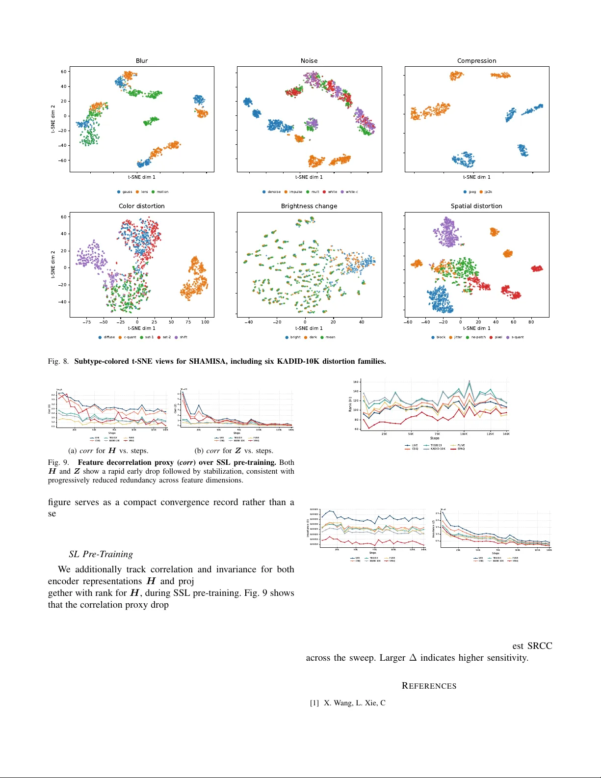
IEEE TRANSA CTIONS ON IMA GE PR OCESSING, SUBMITTED FOR REVIEW 1 SHAMISA: SHAped Modeling of Implicit Structural Associations for Self-supervised No-Reference Image Quality Assessment Mahdi Naseri and Zhou W ang Abstract —No-Reference Image Quality Assessment (NR-IQA) aims to estimate perceptual quality without access to a r eference image of pristine quality . Learning an NR-IQA model faces a fundamental bottleneck: its need for a lar ge number of costly human perceptual labels. W e propose SHAMISA, a non- contrastive self-supervised framework that learns from unlabeled distorted images by leveraging explicitly structur ed relational supervision. Unlike prior methods that impose rigid, binary similarity constraints, SHAMISA introduces implicit structural associations, deﬁned as soft, controllable relations that are both distortion-aware and content-sensitive, inferred from synthetic metadata and intrinsic feature structure. A key innovation is our compositional distortion engine, which generates an un- countable family of degradations from continuous parameter spaces, grouped so that only one distortion factor varies at a time. This enables ﬁne-grained control over representational similarity during training: images with shared distortion patterns are pulled together in the embedding space, while severity variations produce structured, predictable shifts. W e integrate these insights via dual-source relation graphs that encode both known degradation proﬁles and emergent structural afﬁnities to guide the learning process throughout training. A conv olutional encoder is trained under this supervision and then frozen for inference, with quality pr ediction performed by a linear r egressor on its featur es. Extensive experiments on synthetic, authentic, and cross-dataset NR-IQA benchmarks demonstrate that SHAMISA achieves strong ov erall perf ormance with improved cross-dataset generalization and rob ustness, all without human quality anno- tations or contrastive losses. Index T erms —blind image quality assessment, self-supervised learning, graph-based representation learning, distortion model- ing, perceptual quality prediction I . I N T R O D U CT I O N I MA GE Quality Assessment (IQA) aims to estimate per- ceptual image quality in line with human opinion. The No- Reference setting (NR-IQA) is especially challenging, as it must operate without reference images or distortion labels. NR-IQA is critical for real-world tasks such as perceptual enhancement [1], image captioning [2], and streaming opti- mization [3]. Howe ver , modeling perceptual quality is difﬁcult due to the complex interplay between distortion types and content [4], [5]. Supervised approaches [6]–[8] rely on exten- siv e human annotations, with KADID-10K [9] alone requiring ov er 300,000 subjectiv e ratings, making them expensiv e and Mahdi Naseri and Zhou W ang are with the Department of Electrical and Computer Engineering, University of W aterloo, W aterloo, ON N2L 3G1, Canada (e-mail: mahdi.naseri@uwaterloo.ca; zhou.wang@uwaterloo.ca). Cor- responding author: Mahdi Naseri. hard to scale. T o address this, recent ef forts turn to self- supervised learning (SSL), using unlabeled distorted images to learn quality-aware representations [10], [11], typically via contrastiv e objectiv es tailored to either content or degradation similarity . Classical SSL methods like SimCLR [12] and MoCo [13], de veloped for classiﬁcation, learn content-centric and distortion-in variant features. Such representations misalign with NR-IQA, where both content and degradation must be modeled. T o bridge this gap, contrastiv e SSL-IQA meth- ods introduce domain-speciﬁc objectives but can suffer from sampling bias because sampled negati ves may include se- mantically related false negati ves [14]–[16]. CONTRIQUE [17] groups images by distortion type and severity , ignoring content. Re-IQA [11], by contrast, uses overlapping crops of the same image to promote content-aware alignment. While each mode captures useful relations, similarity is enforced either across content or across distortions, but not both. This leads to scattered embeddings for similarly degraded images with different content [18]. ARNIQA [18] learns a distortion manifold by aligning representations of similarly de graded images, irrespective of content. Y et, such approaches rigidly collapse embeddings without accounting for perceptual effects like masking [4], where content alters perceived quality . In practice, perceptual similarity depends jointly on both distor- tion se verity and image content, a dependency that current SSL-IQA models fail to capture in a ﬂexible, scalable manner . W e propose SHAMISA ( SHA ped M odeling of I mplicit S tructural A ssociations), a non-contrasti ve self-supervised framew ork that addresses this challenge by learning represen- tations jointly sensiti ve to both distortion and content through explicitly constructed relation graphs. “SHAped Modeling” refers to graph-based relational supervision, whereas “Im- plicit Structural Associations” denote the latent perceptual relations encoded in these graphs, providing ﬁner control ov er similarity learning than prior SSL-IQA methods that treat distorted views uniformly . SHAMISA draws inspiration from ExGRG [19], which introduced explicit graph-based guidance for self-supervised learning in the graph domain. In contrast, SHAMISA extends this idea to visual data, where quality prediction depends on ﬁne-grained perceptual v aria- tions. Prior methods implicitly impose sparse relational struc- tures, resulting in disconnected or inconsistent supervision, which SHAMISA addresses through e xplicitly shaped relation graphs. At the core of SHAMISA is a compositional distortion IEEE TRANSA CTIONS ON IMA GE PR OCESSING, SUBMITTED FOR REVIEW 2 engine that generates inﬁnite compositional de gradations from continuous parameter spaces. Each mini-batch is built from reference images that form distortion composition groups where only one degradation factor varies, enabling controlled sampling across content, distortion type, and sev erity . From this, we b uild two categories of relation graphs: (i) Metadata- Driven Graphs , which encode pairwise similarity based on distortion metadata, encouraging images with similar degra- dations to lie close in the learned manifold while inducing controlled representational shifts as distortion severity varies; and (ii) Structurally Intrinsic Graphs , constructed from the latent feature space using k -nearest neighbors (kNN) and deep clustering. These graphs supervise a non-contrastive VICReg- style objectiv e with graph-weighted in variance. W ith stop- gradient applied to graph construction, each iteration builds relation graphs from the current representations and updates the model under the resulting objective in a single optimization step. SHAMISA uniﬁes content-dependent and distortion- dependent learning within a single relational framework, generalizing the rigid pairing schemes used in prior SSL-IQA methods. At test time, the learned encoder is frozen and paired with a linear regressor to predict quality scores. SHAMISA achieves strong performance across both synthetic and authentic datasets without requiring human quality labels or contrastive objectiv es. Our main contributions are: 1) W e introduce SHAMISA , a non-contrasti ve self- supervised framew ork for NR-IQA that encodes both distortion-aware and content-aware information into a shared representation space via explicit relational super- vision. 2) W e propose a distortion engine that generates compo- sitional groups with controlled variation, enabling ﬁne- grained similarity learning across distortion factors and content. 3) W e develop a dual-source relation graph construction strategy that combines Metadata-Driv en Graphs based on known degradation metadata and Structurally Intrin- sic Graphs deriv ed from the ev olving feature space, trained with a stop-gradient alternating update that cou- ples on-the-ﬂy graph construction with representation learning. 4) SHAMISA generalizes the rigid pairing schemes used in prior SSL-IQA methods within a uniﬁed graph-weighted in variance framework and achiev es strong overall per- formance across synthetic, authentic, and cross-dataset benchmarks, including the strongest overall six-dataset av erage among the compared SSL methods, together with improved robustness and transfer . I I . R E L A T E D W O R K A. T raditional and Supervised NR-IQA No-Reference Image Quality Assessment (NR-IQA) aims to estimate perceptual image quality without access to pristine references. Traditional methods rely on handcrafted features deriv ed from Natural Scene Statistics (NSS), modeling dis- tortions as de viations from expected regularities. Examples include BRISQUE [20], NIQE [21], DIIVINE [22], and BLI- INDS [23], while CORNIA [24] and HOSA [25] construct codebooks from local patches. Though effecti ve on synthetic distortions, these models often fail on authentically distorted images due to a lack of semantic awareness. Supervised NR-IQA models typically use pre-trained CNNs (e.g., ResNet [26]) to extract deep features, which are mapped to quality scores via regression. T echniques like HyperIQA [7], RAPIQUE [27], and MUSIQ [28] adapt neural architec- tures for perceptual modeling. P aQ-2-PiQ [29] incorporates both image- and patch-lev el quality labels. Others like DB- CNN [6] and PQR [30] combine multiple feature streams. Howe ver , such methods require large-scale and costly human annotations, limiting scalability and generalization. B. Self-Supervised Learning for NR-IQA Self-supervised learning (SSL) enables representation learn- ing from unlabeled data. Contrastive methods lik e SimCLR [12] and MoCo [13] rely on sampled negati ves, which can introduce false negati ves and sampling bias when semanti- cally related samples are treated as negati ves [14]–[16]. Non- contrastiv e methods like VICRe g [31] a void negati ves through in variance and decorrelation. In graph domains, ExGRG [19] introduces explicit relation graphs for SSL, combining domain priors and feature structure. SHAMISA adopts a similar induc- tiv e bias but applies it to NR-IQA, where perceptual similarity depends jointly on content and degradation. Recent SSL-IQA w orks adapt these paradigms to quality prediction. CONTRIQUE [17] clusters samples with similar distortion types into classes, learning quality-aware embed- dings. QPT [10] aligns patches under shared distortion as- sumptions. Re-IQA [11] uses two encoders: one pre-trained for content-speciﬁc features and another trained for distortion- speciﬁc features. Their outputs are concatenated and fed to a single linear regressor . This assumes that a shallow fusion layer can reco ver complex content-distortion interactions from separately learned streams. Re-IQA may therefore under- represent content-distortion interactions, e ven though these interactions play a central role in perceptual quality assessment rather than being ev aluated in isolation [32], [33]. ARNIQA [18] instead aligns representations of images degraded equally , disregarding content. While it captures dis- tortion similarity , it rigidly enforces uniform proximity and ignores perceptual effects introduced by content. In contrast, SHAMISA learns a uniﬁed representation space that respects both distortion and semantic structure, using two complemen- tary relation graphs. A metadata-driv en graph and a struc- turally intrinsic graph together encode distortion-aw are sim- ilarity and perceptual afﬁnities across content. This provides soft, ﬁne-grained constraints that generalize prior methods as special cases. C. Compositional Distortion Modeling and Relational Super- vision Degradation engines are central to SSL-IQA training. Prior models apply a limited set of discrete distortions or ﬁxed IEEE TRANSA CTIONS ON IMA GE PR OCESSING, SUBMITTED FOR REVIEW 3 composition rules [10], [11]. ARNIQA, for example, applies sequential distortions with ﬁxed sampling schemes but lacks structured sampling for controlled variation. RealESRGAN [1] follows a ﬁxed distortion sequence from predeﬁned groups. Such engines offer limited degradation di versity and do not support relational supervision. SHAMISA introduces a compositional distortion engine that generates continuously parameterized degradations with uncountable v ariation. W e partition each mini-batch into tiny- batches (small, ﬁx ed-size subsets). Each tiny-batch contains distortion composition groups in which only one degrada- tion factor varies, enabling precise control over sev erity and type. This supports precise metadata generation for graph construction. Unlike prior works that enforce binary or ﬁxed similarity constraints, SHAMISA enables structured shifts in representation space by applying soft supervision from graph relations. Similar samples lie closer, while severity variation introduces gradual transitions. Combined with its dual-graph relational supervision, SHAMISA learns distortion-aware, content-sensiti ve embed- dings in a non-contrasti ve setting. By decoupling quality learn- ing from rigid class labels and negati ve sampling, SHAMISA offers a scalable and generalizable framework for NR-IQA without relying on human quality annotations or con ventional augmentation heuristics. I I I . M E T H O D As illustrated in Fig. 1, SHAMISA combines structured distortion generation with dual-source relational supervision to learn quality-aware features in a non-contrasti ve setting. W e then transfer the learned encoder to NR-IQA by freezing backbone representations and ﬁtting a lightweight re gressor , so downstream performance reﬂects representation quality rather than head complexity . A. Overview and SSL F ormulation for NR-IQA W e pre-train a ResNet-50 encoder f θ with a 2-layer MLP projector g ψ on unlabeled images degraded online by our distortion engine, optimizing a VICReg-style non-contrastiv e objectiv e [31] to av oid negati ve sampling and its sampling-bias issues [14]. After this self-supervised pre-training, we discard g ψ , freeze f θ (nev er ﬁne-tune), and train a linear regressor on the frozen features for quality prediction. a) T ensorized batch construction: Let N ref denote the number of reference images per mini-batch and N comp the number of distortion compositions applied to each reference image (Sec. III-B). W e take one random crop per pristine image to form R s ∈ R N ref × 3 × H in × W in . Sampling N comp compositions { χ d } N comp d =1 yields distorted sets X ( d ) = χ d ( R s ) ∈ R N ref × 3 × H in × W in , d = 1 , . . . , N comp . W e concatenate references and all distorted sets: X = [ R s ; X (1) ; . . . ; X ( N comp ) ] ∈ R N × 3 × H in × W in , N = N ref ( N comp + 1) . (1) Representations H and Embeddings Z are H = f θ ( X ) ∈ R N × d h , Z = g ψ ( H ) ∈ R N × d z . Human opinion scores are used only for the regression head after pre-training. B. Compositional Distortion Engine A distortion function is one atomic degradation from KADID-10K with 24 functions across 7 categories (Brightness change, Blur, Spatial, Noise, Color , Compression, Sharpness & Contrast) [9]. A distortion composition in SHAMISA is an or dered composition of multiple distortion functions with at most one function per category , applied sequentially . Unlike prior SSL-IQA setups based on discrete se verity grids [10], [18], SHAMISA samples continuous sev erities, yielding an uncountable family of compositions. Order is perceptually consequential, hence we randomize it. In practice each iter- ation uses a ﬁnite N comp , but randomization across iterations explores novel compositions, and continuous lev el dif ferences are exploited later by our relation graphs. a) Severity calibration: F or each distortion function f m we map its nativ e parameter domain [ λ min m , λ max m ] into [0 , 1] via a piecewise-linear calibration ρ m : [ λ min m , λ max m ] → [0 , 1] obtained by linearly interpolating the discrete intensities used in [9]. This yields comparable per-function normalized sever - ities. During sampling we operate in the normalized space; if needed, we recover nativ e parameters by ρ − 1 m . b) Sampling a composition: For each distortion com- position we sample a tuple ( M , S, f , π , λ ) where: M ∼ Unif { 1 , . . . , M d } is the number of distortion functions in the composition with at most one per category; S ⊂ { 1 , . . . , 7 } is a size- M subset indexing the sev en KADID-10K dis- tortion categories, sampled uniformly without replacement; f = ( f 1 , . . . , f M ) picks one function per category in S ; π is a permutation of { 1 , . . . , M } sampled uniformly indicating the application order; and λ = ( λ 1 , . . . , λ M ) ∈ [0 , 1] M are per-function normalized sev erities sampled i.i.d. by drawing ϵ m ∼ N (0 , 0 . 5 2 ) and setting λ m = min(1 , | ϵ m ) , where [0 , 1] M is the M -dimensional unit hypercube. Giv en an input image x , let θ m : = ρ − 1 m ( λ m ) and write f m ( · ; θ m ) . The composed degradation is C ( x ; π , f , λ ) =  f π ( M ) ( · ; θ π ( M ) ) ◦ · · · ◦ f π (1) ( · ; θ π (1) )  ( x ) . (2) 1) Single-factor variation and trajectories: Each mini- batch is partitioned into B tiny-batches; we use [ n ] : = { 1 , . . . , n } for index ranges, so i ∈ [ B ] indexes tiny- batches. In tin y-batch i , select R references { r i,j } R j =1 and instantiate C distortion composition groups . For the k -th composition gr oup ( k ∈ [ C ] ), sample a base composition ( M i,k , S i,k , f i,k , π i,k , λ (0) i,k ) , where λ (0) i,k ∈ [0 , 1] M i,k is the base sev erity vector . Choose exactly one varying coor dinate m ⋆ ( i, k ) ∈ { 1 , . . . , M i,k } , that is, exactly one distortion function whose level will vary within the composition group, and generate L severity le vels { s ( l ) i,k } L l =1 ⊂ [0 , 1] . W e dra w IEEE TRANSA CTIONS ON IMA GE PR OCESSING, SUBMITTED FOR REVIEW 4 (1) Self-supervised Pre-training Dual-source Graphs Metadata-Driven Graphs Pristine Images Compositional Distortion Engine Distortion Metadata Projector Head Structurally Intrinsic Graphs Multi-source Aggregator Graph-weighted SSL Objective (2) Downstream NR-IQA T est Images Linear Head Encoder Frozen Encoder Predicted Quality Scores Fig. 1. Overview of the proposed SHAMISA framework. (1) Self-super vised pre-training: pristine images are transformed by a compositional distortion engine to form a mini-batch X and distortion metadata; the encoder f θ and projector g ψ produce representations H and embeddings Z used to construct dual-source relation graphs (metadata-driven and structurally intrinsic), which are aggreg ated by a multi-source aggreg ator Φ into G and optimize a graph- weighted SSL objecti ve. (2) Downstream NR-IQA: we freeze f θ and train a lightweight regressor on top of H to predict quality scores. each level i.i.d. as s ( l ) i,k = min(1 , | ϵ ( l ) | ) with ϵ ( l ) ∼ N (0 , 0 . 5 2 ) . Deﬁne the per-le vel sev erities component-wise by ( λ ( l ) i,k ) m = ( ( λ (0) i,k ) m , m  = m ⋆ ( i, k ) , s ( l ) i,k , m = m ⋆ ( i, k ) . This single-factor scheme varies one distortion function while holding the others ﬁxed, producing controlled severity varia- tion that isolates that function’ s ef fect in the learned represen- tation. Formally , applying the lev el- l composition in group k to reference r i,j yields the distorted image x i,j,k,l = C  r i,j ; π i,k , f i,k , λ ( l ) i,k  , i ∈ [ B ] , j ∈ [ R ] , k ∈ [ C ] , l ∈ [ L ] . (3) Consequently , the mini-batch contains N ref = B R references and each reference receives N comp = C L compositions, with sampling performed independently for each tiny-batch. C. Explicit Relation Graphs and Graph-weighted VICRe g W e adopt the v ariance and cov ariance regularizers of VI- CReg [31] and replace its augmentation-paired inv ariance term L inv with a graph-weighted variant L ′ inv , in the spirit of explicitly generated relation graphs [19]: L v ar = d z X t =1 max  0 , 1 − q Co v( Z ) t,t  , (4) L cov = d z X t =1 d z X u =1 u  = t Co v( Z ) 2 t,u , (5) L inv = X ( i,j ) ∈A   Z i,. − Z j,.   2 2 , (6) L ′ inv = N X i =1 N X j =1 G i,j   Z i,. − Z j,.   2 2 . (7) Here A ⊆ [ N ] × [ N ] denotes the set of augmentation positi ves, and G ∈ [0 , 1] N × N is the weighted adjacency matrix of a soft relation graph (Sec. III-F), where each entry speciﬁes how strongly the corresponding pair is encouraged to remain in variant. These soft, controllable entries of G instantiate the implicit structural associations, encoding relational cues that jointly capture content and distortion. Intuiti vely , L v ar enforces a minimum per-dimension v ariance to av oid collapse, L cov decorrelates dimensions, and L ′ inv brings together embeddings proportionally to relational strengths encoded by G . In con- trast, L inv uses a rigid binary set A of augmentation positiv es. IEEE TRANSA CTIONS ON IMA GE PR OCESSING, SUBMITTED FOR REVIEW 5 When G is the binary indicator of A (i.e., G i,j = 1 iff ( i, j ) ∈ A and 0 otherwise), Eq. 7 reduces to VICReg’ s original inv ariance in Eq. 6. Our self-supervised pre-training objectiv e is L ssl = α L v ar + β L cov + γ L ′ inv . (8) SHAMISA remains non-contrastive : we do not use negativ es and instead prev ent collapse via the v ariance-covariance terms [31], rather than through negati ve pairs as in contrasti ve methods [12]. a) Relation to prior positives: Cosine inv ariance under- lies InfoNCE in SimCLR [12]. W ith ℓ 2 -normalized features, ∥ a − b ∥ 2 2 = 2 (1 − cos( a, b )) , so Euclidean and cosine in- variances are equi valent up to scaling. Thus, prior in v ariances that rely on rigid binary pairings become special cases of SHAMISA ’ s soft graph-weighted inv ariance. ARNIQA pairs images with the same distortion type and le vel across dif ferent contents [18]; Re-IQA pairs ov erlapping crops of the same image (content-driv en) [11]; CONTRIQUE uses synthetic dis- tortion classes or instance discrimination for UGC [10], [17]. Each choice is recovered by setting G to the corresponding sparse binary adjacency . b) Why an e xplicit G ? Laplacian Eigenmap view: In two- view augmentation setups, the augmentation graph splits into exactly N / 2 disconnected components, so its Laplacian has N / 2 zero eigen values [34]. Allo wing soft cross-component edges in G alleviates this rank deﬁciency and yields a better posed in variance term [19]. Alternating update view: W e construct G from the current representations to deﬁne soft relational targets, then update f θ and g ψ by minimizing Eq. 8. A stop-gradient on the graph inputs, deﬁned formally in Sec. III-F, lets graph construction and parameter updates be ex ecuted in a single optimization step [19], [35]. D. Metadata-Driven Graphs W e con vert engine metadata into soft relational weights that shape the embedding space through two complementary effects. Within a given content, similarity to the pristine anchor decreases smoothly as se verity increases. Across contents, samples from the same distortion composition group remain neighbors when their sev erities are close. W e next deﬁne two monotone maps ϕ, ˆ ϕ : [0 , 1] → [0 , 1] , with ϕ ′ ( u ) ≤ 0 and ˆ ϕ ′ ( u ) ≤ 0 , that con vert a normalized sev erity or se verity gap into a similarity weight. For simplicity , we set ϕ ( u ) = ˆ ϕ ( u ) = exp( − κu ) ; both maps are bounded in [0 , 1] and strictly decreasing in u . 1) Refer ence-distorted graph G rd : Recall that in tiny-batch i and group k , m ⋆ ( i, k ) is the varying function and λ ( l ) i,k ∈ [0 , 1] M i,k is the level- l severity vector . W e assign an edge from each reference to each of its degraded versions: G rd  r i,j , x i,j,k,l  = ϕ  ( λ ( l ) i,k ) m ⋆ ( i,k )  . (9) Intuition. Small severities yield ϕ ≈ 1 and keep mild degrada- tions near the pristine anchor; lar ge sev erities dri ve ϕ → 0 , allowing strong degradations to mov e a way . This produces smooth, severity-a ware attraction without collapse. 2) Distorted-distorted graph G dd : W ithin the same distor- tion composition group ( i, k ) , deﬁne the 1D sev erity gap δ i,k ( l, l ′ ) =   s ( l ) i,k − s ( l ′ ) i,k   ∈ [0 , 1] , and, for any j, j ′ ∈ [ R ] , deﬁne the edge weight between two distorted images whose contents may dif fer as G dd  x i,j,k,l , x i,j ′ ,k,l ′  = ˆ ϕ  δ i,k ( l, l ′ )  . (10) Intuition. Nearby sev erity lev els attract; distant lev els do not. This ties together similarly degraded images r egar dless of content , complementing G rd . T o a void density , we apply a global T op- K d sparsiﬁer: G dd ← F K d ( G dd ) , where F K d retains the K d largest entries in the whole matrix and zeros the rest. 3) Refer ence-r eference graph G rr : W e weakly connect pristine images across contents to stabilize a common high- quality anchor: G rr  r i,j , r i ′ ,j ′  = w rr , w rr ∈ (0 , 1] . (11) Intuition. This graph builds a coherent pristine neighborhood across contents without forcing content collapse; variance- cov ariance re gularizers pre vent trivial solutions while these links stabilize a shared high-quality anchor in the representa- tion space. The three metadata graphs provide severity-awar e , content- awar e soft relations that are fed to the ov erall relation aggre ga- tion (Sec. III-F) and used inside the graph-weighted inv ariance term (Eq. 7) to shape quality-sensiti ve embeddings. E. Structurally Intrinsic Graphs Beyond metadata, we inject emerg ent structure from the ev olving representation space. These graphs encourage local manifold smoothness and global prototype or ganization, com- plementing the metadata graphs. 1) kNN r elation graph: Compute cosine similarities on encoder features H : S H i,j = H ⊤ i,. H j,. ∥ H i,. ∥ 2 ∥ H j,. ∥ 2 . Form the kNN graph by keeping, for each sample, the top k n similarity scores and removing self-connections: G k = F k n ( S H ) ∈ R N × N , (12) where F k n retains the largest k n entries in each row of S H and zeros the rest. Intuition. Deep features are well correlated with perceptual similarity [36]; thus nearest neighbors in H deﬁne perceptu- ally coherent local neighborhoods. G k promotes local smooth- ness of the embedding with respect to this current geometry . IEEE TRANSA CTIONS ON IMA GE PR OCESSING, SUBMITTED FOR REVIEW 6 2) O T -based clustering guidance: Following ExGRG [19], we adapt optimal-transport (OT) clustering guidance to IQA. Let C ∈ R K × d h be K trainable prototypes and A ∈ R N × K the soft assignments A j,k = exp( H ⊤ j,. C k,. /τ c ) P k ′ exp( H ⊤ j,. C k ′ ,. /τ c ) . (13) Balanced tar gets T ∈ R N × K are obtained by a Sinkhorn- Knopp solv er with entropy regularization [37], which enforces approximately uniform cluster marginals per mini-batch [38], [39]. For probability vectors t , a ∈ [0 , 1] K with P K k =1 t k = P K k =1 a k = 1 , we deﬁne the cross-entropy CE( t , a ) : = − K X k =1 t k log a k . For notational conv enience, we write T x i,j,k,l and A x i,j,k,l for the rows of T and A associated with distorted image x i,j,k,l in Eq. 3. The O T loss has two contributions, L ot = 1 N N X n =1 CE  T n,. , A n,.  + 1 |P | X ( u,v ) ∈P CE  T u,. , A v ,.  , (14) P =  ( x i,j,k,l , x i,j ′ ,k,l ) : i ∈ [ B ] , k ∈ [ C ] , l ∈ [ L ] , j  = j ′  . where N is the mini-batch size in Eq. 1. The ﬁrst term aligns each sample’ s assignment to its own balanced target ov er all N images in the mini-batch. The set P contains cross- content distorted-image pairs that share the same tiny-batch i , composition group k , and sev erity level l . The second term av erages the corresponding cross-entropy over these pairs. Soft assignments A provide graded membership probabil- ities, which reduce premature hard assignments and allo w clusters to form more ﬂexibly . From A we compute an assignment-afﬁnity matrix S A i,j = X k A i,k log A j,k , then normalize entries and apply a global sparsity limit to obtain the relation graph G o = F K g  norm( S A )  ∈ R N × N , (15) where norm maps the matrix entries into [0 , 1] via global min- max normalization, and F K g keeps the globally largest K g entries, zeroing the rest. Intuition. OT -based guidance shapes the global topology by encouraging samples with similar prototype memberships to remain close across contents, while soft assignments preserve uncertainty during cluster formation. Prototypes C and the encoder f θ (hence H ) are updated by gradients of L ot together with the ov erall objectiv e each iteration; A and T are recomputed from the current features. F . Multi-Sour ce Aggr egation with Stop-Gradient Let S G = { G rd , G dd , G rr , G k , G o } . W e apply a stop-gradient to each source and combine them with learned nonnegati ve coefﬁcients: ˜ G ( i ) = sg  G ( i )  , (16) G = X G ( i ) ∈ S G ω i ˜ G ( i ) , ω i ≥ 0 , X i ω i = 1 , (17) where sg ( · ) is the stop-gradient operator (identity in forward, zero gradient in backward). The weights ω are produced by a lightweight hypernetwork Φ [19], [40] from simple per-graph statistics, ω = softmax  Φ  { ζ ( i ) } T i =1   , ζ ( i ) =  sum( G ( i ) ) , nnz( G ( i ) )  , (18) where T = | S G | , { ζ ( i ) } T i =1 denotes stacking the per-graph statistics over sources, sum( · ) is the total edge weight (con- nection mass), and nnz( · ) is the number of nonzero entries (sparsity). This hypernetwork aggregates an arbitrary set of sources online, adapting ω as the graphs ev olve during train- ing. The two statistics are inexpensiv e, scale-agnostic proxies for strength and cover age of each source, providing a practical signal for allocating weight without hand-tuning. G. T raining Details W e maintain sparse relation graphs via the pruning op- erators F k n (T op- k per row) and F K d , F K g (global T op- K ). The graph-weighted in v ariance L ′ inv is then ev aluated as P ( i,j ): G ij > 0 G ij ∥ Z i,. − Z j,. ∥ 2 2 , i.e., only ov er nonzero edges rather than all N 2 pairs; this respects sparsiﬁcation and reduces computation. W e include the graph regularizer R graph = − X i,j G 2 i,j , to encourage nontri vial mass on the retained edges after sparsiﬁcation. Under the simplex constraint on ω , this fav ors informativ e retained edge weights instead of vanishing graph mass. Our construction choices keep all graph entries in [0 , 1] , which avoids uncontrolled saturation. H. End-to-End Optimization and Regr ession Protocol The full objective is L total = L ssl + η L ot + ξ R graph . (19) In each iteration, we construct G from the current repre- sentations, then update the encoder f θ , projector g ψ , the prototype parameters, and the aggregation hypernetwork Φ by minimizing Eq. 19 while applying stop-gradient through G . After pre-training, g ψ is discarded and f θ is frozen; we then train a linear regressor on the encoder features H to predict human opinion scores. I V . E X P E R I M E N TA L E V A L UAT I ON W e ev aluate SHAMISA on standard NR-IQA benchmarks with a linear-probe protocol [11], [17], [18], report SRCC and PLCC, and study within-dataset performance, cross-dataset transfer , gMAD diagnostics, representation visualizations, ab- lations, and a full-reference extension. IEEE TRANSA CTIONS ON IMA GE PR OCESSING, SUBMITTED FOR REVIEW 7 A. Setup a) Backbone and prete xt: W e initialize a ResNet-50 encoder f θ from ImageNet and pre-tr ain it self-supervised with L total (Eq. 19), which couples VICReg-style vari- ance/cov ariance terms with a graph-weighted in variance term. A 2-layer MLP projector g ψ is used only during pre-training. Unlabeled inputs are degraded online by the compositional distortion engine (Sec. III). Unless otherwise noted, training uses sparse relation graphs G rd , G dd , G rr , G k , G o aggregated by Φ . After pre-training, g ψ is discarded and f θ is frozen for all ev aluations. b) T raining details: W e pre-train for one epoch over the 140k KADIS reference images with SGD. Encoder and pro- jector dimensions are d h =2048 and d z =256 . Each update uses B =2 tiny-batches, R =3 references, C =4 composition groups, and L =5 severity lev els, gi ving N ref = B R =6 , N comp = C L =20 , and N = N ref ( N comp + 1)=126 in Eq. 1. Distortion generation uses M d =7 . Graph sparsity and O T settings are k n =31 , K d =4096 , K =32 , and τ c =0 . 1 ; for the O T graph, the effec- tiv e global sparsiﬁcation budget scales with mini-batch size through K g =8 N . Crop size is 224 × 224 . Remaining details are listed in Supplementary Appendix A. B. Datasets and Evaluation Pr otocol a) Pr e-training data: Follo wing ARNIQA [18], we use the 140k pristine images from KADIS [9] as content sources to enable a fair comparison under a shared pre-training cor- pus. W e generate degradations online with our compositional distortion engine. b) Evaluation datasets: W e include both synthetic and in-the-wild benchmarks. Synthetic: LIVE [41], CSIQ [42], TID2013 [43], KADID-10K [9]. In-the-wild: FLIVE [29], SP A Q [44]. Brief dataset statistics are a vailable in Supple- mentary Appendix D. c) Pr otocol: W e follow SSL-IQA practice [11], [17], [18]. For LIVE, CSIQ, TID2013, KADID-10K, and SP A Q, we create 10 train/v al/test splits, using reference-disjoint sampling on the synthetic datasets and random 70/10/20 splits on SP A Q. For FLIVE, we use the of ﬁcial split [29]. W e train an ℓ 2 ridge regressor [45] on frozen features and select α ridge from a log-spaced grid of 100 v alues in [10 − 3 , 10 3 ] by maximizing median validation SRCC across the av ailable splits. At test time, we extract features at full and half scale and concatenate [17], then av erage predictions ov er ﬁve deterministic crops per image (four corners and center) [10]. W e report the median ov er the repeated splits where applicable. PLCC is computed after the standard four-parameter logistic mapping [46]. C. Compar ed Methods W e compare against traditional NR-IQA (BRISQUE [20], NIQE [21]), codebook models (CORNIA [24], HOSA [25]), and deep supervised NR-IQA (DB-CNN [6], HyperIQA [7], TReS [8], Su et al. [47]). W e also include SSL-IQA baselines CONTRIQUE [17], Re-IQA [11], and ARNIQA [18], match- ing the methods reported in T able I. D. W ithin-Dataset P erformance T able I shows that SHAMISA attains the best SRCC and PLCC on LIVE, CSIQ, and TID2013, while remaining com- petitiv e on KADID-10K, FLIVE, and SP A Q under the frozen- encoder linear-probe protocol. On KADID-10K, SHAMISA ranks behind CONTRIQ UE but ahead of ARNIQA, which is consistent with KADID-10K closely matching the syn- thetic distortion families emphasized by CONTRIQUE’ s pre- training scheme. For authentic images, SHAMISA is second on FLIVE and remains competiti ve on SP A Q, trailing Re- IQA by a narrow margin. This suggests a stronger balance between synthetic and authentic performance than meth- ods that are markedly stronger on only one side. Overall, SHAMISA achiev es the strongest six-dataset av erage SRCC and PLCC among the SSL methods reported here, with av erage SRCC/PLCC of 0.886/0.904. W e attribute these gains to two factors: a compositional distortion engine that forms single-factor severity trajectories, and dual-source relation graphs that fuse metadata-driv en and structure-intrinsic relations within a graph-weighted VICReg objectiv e. These gains do not come from a materially larger training budget. Under the same KADIS (140k) protocol on an NVIDIA H100 80GB (HBM3), end-to-end pre-training plus e v aluation on the six NR-IQA benchmarks takes approxi- mately 12.5 hours for ARNIQA and 13.5 hours for SHAMISA. Re-IQA is more training-intensiv e, as it additionally trains a content encoder on ImageNet and a separate quality encoder with large augmentation schedules. E. Cr oss-Dataset T ransfer a) Cr oss-dataset transfer: T able II shows that SHAMISA attains the best SRCC on 9 of the 12 synthetic transfer directions, ranks second on 2 more, and remains competitiv e on the remaining case. Relati ve to ARNIQA, the clearest gains appear when the source dataset cov ers fewer distortion types, such as LIVE or CSIQ, and the target is more di verse, such as TID2013 or KADID-10K. This pattern is visible in LIVE → CSIQ, LIVE → TID2013, CSIQ → TID2013, and TID2013 → KADID-10K, suggesting that the learned representation aligns distortion structure across contents in a way a linear regressor can exploit. The main exception is LIVE → KADID-10K, where ARNIQA and CONTRIQUE retain an advantage. KADID-10K → LIVE is another difﬁcult direction, where HyperIQA remains strongest and SHAMISA ranks second. This pattern is consistent with LIVE being smaller and perceptually milder , leaving less headroom for severity-a ware supervision. b) Pr otocol: W e follow the standard SSL-IQA linear- probe setting: the encoder is frozen; we train a ridge regressor on the train split of the source dataset, select its regularization on the source v al split, and e valuat e zero-shot on the target test split with identical multi-scale features and ﬁve-crop pooling. W e report the median ov er 10 reference-disjoint splits. This transfer style mirrors practical deplo yment. A large pool of unlabeled images is used for SSL pre-training, and only a small labeled set from a related source dataset is av ailable to ﬁt a lightweight head. The model must then generalize to a IEEE TRANSA CTIONS ON IMA GE PR OCESSING, SUBMITTED FOR REVIEW 8 T ABLE I P E RF O R M AN C E C OM PA R IS O N O N S Y N T HE T I C AN D I N - TH E - W IL D N R -I Q A DAT A S ET S . W E R E P O RT S R C C A ND P L C C. B E S T AN D S E CO N D - BE S T P ER C O LU M N A RE B O L D A N D U N DE R L IN E D . P RI O R N UM B E R S A R E T A K EN F RO M T H EI R PAP E R S O R P U B LI C C O D E W H E R E A V A I L AB L E [ 11 ] , [ 17 ] , [ 1 8] . Synthetic distortions Authentic distortions Method T ype LIVE CSIQ TID2013 KADID-10K FLIVE SP AQ A verage SRCC PLCC SRCC PLCC SRCC PLCC SRCC PLCC SRCC PLCC SRCC PLCC SRCC PLCC BRISQUE [20] Handcrafted 0.939 0.935 0.746 0.829 0.604 0.694 0.528 0.567 0.288 0.373 0.809 0.817 0.652 0.703 NIQE [21] Handcrafted 0.907 0.901 0.627 0.712 0.315 0.393 0.374 0.428 0.211 0.288 0.700 0.709 0.522 0.572 CORNIA [24] Codebook 0.947 0.950 0.678 0.776 0.678 0.768 0.516 0.558 – – 0.709 0.725 – – HOSA [25] Codebook 0.946 0.950 0.741 0.823 0.735 0.815 0.618 0.653 – – 0.846 0.852 – – DB-CNN [6] Supervised 0.968 0.971 0.946 0.959 0.816 0.865 0.851 0.856 0.554 0.652 0.911 0.915 0.841 0.870 HyperIQA [7] Supervised 0.962 0.966 0.923 0.942 0.840 0.858 0.852 0.845 0.535 0.623 0.916 0.919 0.838 0.859 TReS [8] Supervised 0.969 0.968 0.922 0.942 0.863 0.883 0.859 0.858 0.554 0.625 – – – – Su et al. [47] Supervised 0.973 0.974 0.935 0.952 0.815 0.859 0.866 0.874 – – – – – – CONTRIQUE [17] SSL+LR 0.960 0.961 0.942 0.955 0.843 0.857 0.934 0.937 0.580 0.641 0.914 0.919 0.862 0.878 Re-IQA [11] SSL+LR 0.970 0.971 0.947 0.960 0.804 0.861 0.872 0.885 0.645 0.733 0.918 0.925 0.859 0.889 ARNIQA [18] SSL+LR 0.966 0.970 0.962 0.973 0.880 0.901 0.908 0.912 0.595 0.671 0.905 0.910 0.869 0.890 SHAMISA (ours) SSL+LR 0.986 0.987 0.981 0.987 0.904 0.919 0.922 0.924 0.610 0.688 0.914 0.920 0.886 0.904 T ABLE II C RO S S - D A TA S ET S R C C ON S Y N T HE T I C NR - I Q A B E N C HM A R KS . B E S T A N D S E C O ND - B ES T P E R ROW A R E BO L D A ND U N D E RL I N ED . B A S E L IN E V A L U ES A R E T A KE N F RO M P RI O R R E PO RT S I N A R N I QA A N D R E - I Q A [ 1 1] , [ 1 8] . Training T esting HyperIQA Su et al. CONTRIQUE Re-IQA ARNIQA SHAMISA LIVE CSIQ 0.744 0.777 0.803 0.795 0.904 0.909 LIVE TID2013 0.541 0.561 0.640 0.588 0.697 0.700 LIVE KADID-10K 0.492 0.506 0.699 0.557 0.764 0.694 CSIQ LIVE 0.926 0.930 0.912 0.919 0.921 0.939 CSIQ TID2013 0.541 0.550 0.570 0.575 0.721 0.729 CSIQ KADID-10K 0.509 0.515 0.696 0.521 0.735 0.711 TID2013 LIVE 0.876 0.892 0.904 0.900 0.869 0.908 TID2013 CSIQ 0.709 0.754 0.811 0.850 0.866 0.870 TID2013 KADID-10K 0.581 0.554 0.640 0.636 0.726 0.779 KADID-10K LIVE 0.908 0.896 0.900 0.892 0.898 0.901 KADID-10K CSIQ 0.809 0.828 0.773 0.855 0.882 0.892 KADID-10K TID2013 0.706 0.687 0.612 0.777 0.760 0.779 (a) SHAMISA, low bin (b) SHAMISA, high bin (c) ARNIQA, low bin (d) ARNIQA, high bin Fig. 2. gMAD on W aterloo Exploration (distorted pool): panels (a,b) use SHAMISA as the defender and panels (c,d) use ARNIQA as the defender . In each panel, the top and bottom images are the attacker-selected pair from the indicated defender-quality bin, with low-bin cases shown in (a,c) and high- bin cases sho wn in (b,d). Supplementary T able VII reports the corresponding top-1 attacker gaps. related b ut distinct tar get without target labels and without adapting normalization statistics to the target dataset. Full details are provided in Supplementary Appendix F . F . gMAD Diagnostic on W aterloo W e use the group maximum dif ferentiation (gMAD) pro- tocol [48] as a pairwise diagnostic on the W aterloo Ex- ploration Database [49] using its distorted image pool (no MOS annotations). F ollowing our standard NR-IQA ev aluation pipeline, we con vert frozen representations into scalar quality 100 50 0 50 100 t-SNE dim 1 100 50 0 50 100 t-SNE dim 2 ARNIQA 100 50 0 50 100 t-SNE dim 1 100 50 0 50 100 SHAMIS A Blur Noise Compr ession Color distortion Brightness change Spatial distortion Sharpness / contrast Fig. 3. t-SNE visualization of image-lev el encoder representations on KADID-10K. W e extract encoder representations H (pre-projector) and av erage across crops to obtain one representation per image, yielding 10,125 image-lev el points. Points are colored by the coarse distortion family using a shared ﬁxed palette. Compared to ARNIQA, SHAMISA exhibits clearer coarse-family structure for sev eral dominant degradation families, while both models sho w ov erlap among visually related families such as brightness and color manipulations. This visualization is a qualitativ e diagnostic and does not af fect the quantitati ve ev aluation protocol. predictions by ﬁtting a ridge regressor on KADID-10K and then apply the resulting predictors to all W aterloo images. Giv en a defender model, we ﬁrst split the pool into equal-count bins based on the defender’ s predicted quality . W ithin a chosen bin, the attacker then selects the image pair with the largest attacker -side score gap while the defender still scores the pair similarly . Supplementary Appendix I giv es the corresponding protocol details. Fig. 2 sho ws representati ve pairs for low and high defender levels in both defender-attack er directions, and Supplementary T able VII reports the corresponding top-1 attacker gaps. In this pairwise W aterloo gMAD comparison with KADID-trained ridge heads, attacker g aps are smaller when SHAMISA is the defender than when ARNIQA is the defender , suggesting tighter within-bin quality consistenc y for SHAMISA in this speciﬁc setting. G. t-SNE Repr esentation V isualization W e visualize the structure of the learned representation space by applying 2D t-SNE [50] to image-lev el encoder representations H on KADID-10K [9]. For each image, we extract H (pre-projector) and average across crops, yielding IEEE TRANSA CTIONS ON IMA GE PR OCESSING, SUBMITTED FOR REVIEW 9 (a) ARNIQA (b) SHAMISA Fig. 4. Manifold visualization with UMAP [51] using encoder representa- tions H extracted from 1,000 pristine KADIS images de graded with Gaussian blur and white noise. For each pristine image we generate 5 blur -only samples, 5 noise-only samples, and all 5 × 5 blur → noise compositions (35 variants per image, 35k total points). Point color is the weighted a verage of blur (red) and noise (yellow) according to their relative intensities; marker opacity increases with total se verity . 10 , 125 points. Fig. 3 colors points by coarse distortion fam- ily using a shared, ﬁx ed palette for fair visual comparison. Both methods separate sev eral major degradation families, but SHAMISA often forms more coherent regions for prominent categories, whereas ARNIQA shows more inter-f amily mixing in the central area. W e provide additional se verity-colored visualizations and subtype-lev el views (by distortion family) in Supplementary Appendix G. Across these plots, separability is strongest for families with distincti ve artifact statistics (e.g., blur , noise, and compression), while brightness-related manipulations remain more entangled and challenging for both models. Overall, these plots are consistent with SHAMISA ’ s pre-training encouraging a representation geometry that is coherent across major distortion families while still preserving ﬁne-grained variation within them. H. UMAP Manifold V isualization W e visualize the distortion manifold induced by two degra- dations and their compositions using UMAP [51]. W e sample 1,000 pristine images from KADIS and generate 35 degraded variants per image: 5 blur -only samples, 5 noise-only samples, and all 5 × 5 blur → noise compositions, where blur is applied before noise. W e then extract pooled encoder features H (pre-projector) with frozen weights and embed them into 2D using identical UMAP hyperparameters across models (Fig. 4). Protocol details are gi ven in Supplementary Appendix H. UMAP is ﬁt independently for each model, so the absolute axes are not aligned across panels. W e therefore compare the internal org anization of each panel, rather than point-by-point coordinates across panels. Across both models, compositions tend to lie closer to the noise re gion, consistent with noise being applied after blur and thus remaining visually dominant in the ﬁnal image. Howe ver , the geometry dif fers markedly between ARNIQA and SHAMISA. The ARNIQA embedding contains a large, diffuse interior region where samples with dif ferent blur -to- noise mixtures overlap strongly , yielding a weak and locally inconsistent color gradient. In contrast, SHAMISA appears to produce a more organized manifold, with clearer bands and a smoother progression from blur-dominated (red) to noise- dominated (yello w) compositions, as well as fe wer ambigu- T ABLE III M AI N A B LAT IO N S . M E D I AN O VE R 1 0 S PL I T S PE R D A TA SE T ; T H EN AVE R AG ED . S RC C s / PL C C s A V E RA GE OVE R S Y NT H E TI C { LIVE , CSIQ , TID2013 , KADID - 10K } , S R CC a / PL C C a OV E R AUT H E NT I C { FLIVE , SP AQ } , A N D S RC C g / PL C C g D EN OT E T H E A V E RAG E OV E R T HE SI X P ER - DA TAS E T M ED I AN SR C C/ P L CC V A LU E S . F U L L A BL ATI O N CATAL O G I S R EP O RTE D I N S U PP L EM E NTA RY T AB L E V II I . V ariant SRCC g PLCC g SRCC a PLCC a SRCC s PLCC s A0: SHAMISA 0.8862 0.9042 0.7620 0.8040 0.9483 0.9543 (A) Aggr egation & re gularization A1: Binary G 0.8767 0.8924 0.7475 0.7821 0.9374 0.9457 A3: No Φ (ﬁxed linear mixture) 0.8759 0.8951 0.7479 0.7896 0.9361 0.9457 (B) Graph sour ces B1: No G o (OT graph) 0.8600 0.8787 0.7661 0.8069 0.8995 0.9092 B7: Metadata only { G rd , G dd , G rr } 0.8467 0.8648 0.7634 0.8010 0.8801 0.8905 B6: G k only 0.7891 0.8018 0.7577 0.7825 0.7922 0.8017 B8: Structure only { G k , G o } 0.8753 0.8961 0.7419 0.7891 0.9387 0.9475 (D) Distortion engine D1: M d =1 0.8775 0.9077 0.7259 0.7684 0.9519 0.9783 D2: Discrete sev erities ( L =5 ) 0.8767 0.8987 0.7456 0.7890 0.9386 0.9518 D4: Fixed order π 0.8587 0.8712 0.7434 0.7668 0.9113 0.9215 (E) Objective diagnostic E1: No L ot 0.7887 0.8009 0.7597 0.7836 0.7904 0.7996 ous mixed-mixture points concentrated in the middle. This qualitativ e diagnostic suggests that SHAMISA more explicitly parameterizes the two distortion ax es under composition: blur and noise vary more smoothly , and with less central mixing than ARNIQA. I. Ablations a) Ablation design: W e ablate SHAMISA along comple- mentary axes that map directly to our main design choices: (A) how we aggregate multi-source relations into the soft matrix G (learned end-to-end mixing Φ vs ﬁxed mixing; regularization), (B) which relation sources are necessary (structure graphs G k , G o vs metadata graphs G rd , G dd , G rr ), (C) how we sparsify the global OT graph (global vs ro w-wise trunca- tion), (D) how the compositional distortion engine deﬁnes the self-supervised training distribution (composition complexity , sev erity modeling, ordering), and (E–F) objective diagnostics that isolate the contribution of O T alignment and se verity- dependent edge weighting. Each v ariant changes only minimal factors relative to the reference conﬁguration (A0). W e ev alu- ate on six NR-IQA datasets (LIVE, CSIQ, TID2013, KADID- 10K, FLIVE, SP A Q) with 10 random splits per dataset, report- ing the median test SRCC/PLCC per dataset, then summariz- ing synthetic and authentic groups separately together with a global comparison score. For readability , T able III highlights the most diagnostic variants; the complete catalog is deferred to Supplementary T able VIII. b) Results and analysis: A0 achiev es SRCC g =0 . 8862 (PLCC g =0 . 9042 ), with SRCC s =0 . 9483 and SRCC a =0 . 7620 . Across all variants (Supplementary T able VIII), three con- sistent trends emer ge that directly support SHAMISA ’ s ke y claims. First, global O T structure is the dominant structural prior : remo ving the O T alignment term (E1) yields the lar gest degradation (SRCC g =0 . 7887 ), and removing the O T -derived global graph G o (B1) causes the strongest drop among single- source remo vals (0.8600). T ogether , these results indicate that SHAMISA ’ s gains are not explained by generic instance-level in variances alone; rather , O T -guided relations enforce long- range consistency that shapes the global geometry of the IEEE TRANSA CTIONS ON IMA GE PR OCESSING, SUBMITTED FOR REVIEW 10 learned quality manifold and is difﬁcult to recov er from local neighborhoods. Second, multi-sour ce r elational supervision is necessary , with structur e and metadata playing complementary r oles . The single-family variants are substantially worse than A0: using only local structure G k (B6) collapses to SRCC g =0 . 7891 , while metadata-only graphs (B7) improv e to 0.8467 but remain far from A0. This separation clariﬁes the contribution of each novelty: structural graphs preserve local neighborhoods that emerge in the ev olving representation space, thereby stabilizing a content-consistent geometry rather than forcing similarity from distortion metadata alone, while metadata graphs inject distortion semantics that are not reliably infer- able from pixels alone, especially under authentic mixtures. Consistent with this view , structure-only { G k , G o } (B8) is competitiv e on synthetic data (SRCC s =0 . 9387 ) but drops on authentic data (SRCC a =0 . 7419 ), highlighting that metadata relations mainly contribute rob ustness to real-world content and capture-device shifts. In contrast, remo ving any single metadata edge type (B3–B5) produces only modest changes, suggesting each metadata relation is individually weak but collectiv ely beneﬁcial. Third, the distortion engine beneﬁts fr om both composition diversity and r ealistic se verity modeling . Restricting composi- tions to a single atomic distortion (D1, M d =1 ) still yields very strong synthetic performance (SRCC s =0 . 9519 ), but it reduces authentic performance (SRCC a : 0.7259 vs 0.7620) and slightly lowers global SRCC relative to A0. This suggests that richer compositions matter for the mixed degradations encountered beyond synthetic benchmarks. Moreover , ﬁxing the composition order (D4) substantially harms performance (SRCC g =0 . 8587 ), directly supporting the need for stochastic composition div ersity to pre vent o verﬁtting to a narrow degra- dation trajectory . Sev erity modeling also matters: discretizing sev erities (D2, L =5 ) reduces SRCC g to 0.8767, suggesting that coarse sev erity quantization weakens the smooth relative- order information that the metadata graphs can exploit. Using uniform severity sampling (D3) also de grades performance slightly (0.8743), consistent with the default se verity sampling fa voring milder distortions and av oiding an ov errepresentation of unrealistic extreme cases. Finally , ablations of relation aggregation indicate that how relations are mix ed matters, b ut the ef fects are necessarily smaller than removing relations entirely . Binarizing G (A1) slightly reduces SRCC g (0.8767), supporting soft relation strengths for graded supervision. Replacing learned mixing Φ with ﬁx ed linear mixing (A3) decreases SRCC g to 0.8759, consistent with Φ learning to reweight heterogeneous relation sources. Removing the graph regularizer R graph (A2) yields only a small drop in SRCC g (0.8813), suggesting that it mainly impro ves stability and calibration rather than acting as a dominant source of the gains. J. Pr e-training Dynamics W e track do wnstream NR-IQA performance during SSL pre-training by periodically freezing the encoder and ﬁtting a lightweight regressor on each target dataset. Frozen check- points are ev aluated every 5000 training steps. Fig. 5 shows 0.95 0.96 0.97 0.98 0.99 1.00 LIVE 0.92 0.94 0.96 0.98 1.00 C SIQ 25K 50K 75K 100K 140K 0.5 0.6 0.7 0.8 0.9 1.0 TID2013 25K 50K 75K 100K 140K 0.84 0.86 0.88 0.90 0.92 0.94 KADID -10K Steps SR CC Fig. 5. SRCC vs. training steps during SSL pre-training (mean with ± std error bars over 10 splits) across representative NR-IQA benchmarks. Curves typically rise early and then saturate, while the best checkpoint can vary by dataset since the SSL objectiv e is not identical to do wnstream SRCC. 64 128 192 256 384 512 0.6 0.7 0.8 0.9 d h 2 4 8 B 3 6 11.98 24 48 22 44 88.37 176 352 5 10 20 31 50 80 k n 128 256 384 512 0.6 0.7 0.8 0.9 d z 0.005 0.01 0.02 0.05 0.1 14 28 57.21 114 228 0 0.25 0.49 1 8 32 64 128 K SR CC LIVE CSIQ TID13 K ADID FLIVE SP A Q Fig. 6. One-at-a-time sweeps around the SHAMISA reference A0, reporting SRCC across six NR-IQA benchmarks in a single merged view . Columns correspond to ( d h , d z ) , ( B , ξ ) , ( α, β ) , ( γ , η ) , and ( k n , K ) , with a shared le gend across all panels. that SRCC impro ves rapidly in the early phase and then saturates across the representativ e benchmark datasets shown here, indicating that the learned representation becomes useful for quality prediction relativ ely early in pre-training. Importantly , the best checkpoint can be dataset-dependent: while some datasets continue to improve or remain stable as pre-training proceeds, others exhibit a mild peak-and-decline behavior , which is expected because the SSL objective is not optimized directly for SRCC on any single benchmark. As a deployment note, when a small labeled v alidation set is av ailable in the target domain, it can be used to select a checkpoint for that domain. Unless stated otherwise, all results reported in T ables I and II use the ﬁxed A0 checkpoint; this section is a diagnostic and is not used for model selection. Additional diagnostic ﬁgures are provided in Supplementary Appendix K. K. Hyperparameter Sensitivity W e analyze hyperparameter sensiti vity by v arying one knob at a time around our A0 conﬁguration while keeping the rest IEEE TRANSA CTIONS ON IMA GE PR OCESSING, SUBMITTED FOR REVIEW 11 ﬁxed. Fig. 6 sho ws that most capacity and graph-construction choices admit broad plateaus: d h , d z , and k n typically yield stable SRCC across a wide range, and increasing K mainly saturates after moderate v alues. In contrast, the O T alignment coefﬁcient η is the most inﬂuential knob across datasets, with the largest SRCC swings on synthetic distortion benchmarks such as TID2013 and KADID-10K, suggesting that overly weak alignment under-utilizes relational guidance, whereas ov erly strong alignment can over -constrain representations. Among VICReg terms, the inv ariance weight γ exhibits the clearest sensitivity , particularly on FLIVE, whereas the vari- ance and cov ariance weights α and β are comparativ ely robust across the tested ranges. Overall, these sweeps indicate that SHAMISA is robust across broad ranges of capacity and graph-design choices, while a smaller set of alignment-related coefﬁcients, especially η and γ , remains important for ﬁne control. Supplementary Appendix L reports the corresponding SRCC sensitivity summary . a) FR extension: W e also propose a full-reference vari- ant, SHAMISA-FR, that reuses the frozen no-reference en- coder and uses the absolute feature dif ference | h ref − h dist | between pristine and distorted images as the regressor input. This variant requires no additional backbone pre-training and attains competitive FR-IQA accuracy; details are provided in Supplementary Appendix E, with the main comparison in Supplementary T able VI. b) Repr oducibility: Additional implementation details, optimization settings, e valuation protocols, and supplemen- tary diagnostics are provided in Supplementary Appendix A, Supplementary Appendix F , Supplementary Appendix K, and Supplementary Appendix L. The project repository is available at https://github.com/Mahdi- Naseri/SHAMISA/. V . C O N C L U S I O N W e presented SHAMISA , a non-contrastive self-supervised framew ork for NR-IQA that learns uniﬁed distortion-aware and content-aware representations. SHAMISA couples a com- positional distortion engine with single-factor variation to gen- erate controllable severity trajectories, and supervises learn- ing through dual-source relation graphs that fuse Metadata- Driv en Graphs with Structurally Intrinsic Graphs. These re- lations driv e a graph-weighted VICReg-style in variance with clustering-guided supervision. In each iteration, we construct the graphs from the current representations and then update the model with stop-gradient. This yields a frozen encoder whose features support accurate quality prediction with a linear regressor . Across synthetic and authentic benchmarks, SHAMISA achiev es the strongest overall average among the SSL methods compared here, with impro ved cross-dataset generalization and stronger gMAD diagnostics, while using no human quality labels during pre-training. A full-reference vari- ant, SHAMISA-FR, reuses the same frozen encoder without additional backbone training and attains competitive FR-IQA accuracy . Future work includes e xploiting the learned topology for blind image restoration and extending the framew ork to video quality assessment. IEEE TRANSA CTIONS ON IMA GE PR OCESSING, SUBMITTED FOR REVIEW 12 Supplementary Material for “SHAMISA: SHAped Modeling of Implicit Structural Associations for Self-supervised No-Reference Image Quality Assessment” Mahdi Naseri and Zhou W ang A P P E N D I X A A R C H I T E C T U R E S A N D O P T I M I Z A T I O N T able IV summarizes the ﬁxed SHAMISA pre-training con- ﬁguration used across all experiments; unless stated otherwise, downstream ev aluation selects the ridge regularization α ridge per dataset on the validation split, as described in Sec. IV -B. Implementation detail for graph construction: diagonal self- edges are removed from all source graphs before aggregation. W e therefore do not use self-in v ariance edges in Eq. 7. A P P E N D I X B C O M P O S I T I O NA L D I S TO RT I O N E N G I N E W e use the compositional engine of Sec. III-B with M d = 7 and per-update structure B = 2 tiny-batches, each with R = 3 pristine references and C = 4 distortion composition groups. Each group forms a single-factor trajectory with L = 5 levels, generating images x i,j,k,l as deﬁned in Eq. 3. Normalized sev erities are sampled i.i.d. by drawing ϵ ∼ N (0 , 0 . 5 2 ) and setting s = min(1 , | ϵ | ) ; within each group, one distortion coordinate varies across L i.i.d. draws { s ( l ) } L l =1 , which are kept in sampled order and are not forced to include either endpoint of the se verity range, while all other coordinates are held at their baseline sampled values. Distortion functions are applied sequentially in a uniformly random order (Eq. 2). A P P E N D I X C E V A L UAT IO N D E T A I L S Follo wing prior SSL-IQA ev aluation practice [11], [17], [18], we use two scales per image (full and half) and ﬁv e deterministic crops per scale [10], [17], with ridge regular - ization selected on the validation split as in Sec. IV -B. W e report the median ov er 10 random splits where applicable. On synthetic datasets, the splits are reference-disjoint follo wing [11], [17], [18]. For FLIVE we use the of ﬁcial split [29], and for SP A Q we use random 70/10/20 splits. PLCC follows the same four-parameter logistic mapping speciﬁed in Sec. IV -B. A P P E N D I X D D A TA S E TS W e e valuate on four synthetic IQA benchmarks and two authentic in-the-wild IQA benchmarks. T able V summarizes the dataset sizes, label types, and split notes used throughout the paper . Among the authentic datasets, FLIVE provides large-scale in-the-wild images with both image-level and patch-le vel qual- ity annotations [29], whereas SP A Q focuses on smartphone photography captured under di verse real-world conditions [44]. For SP A Q, we resize the shorter side to 512 as in [44]. A P P E N D I X E S H A M I S A - F R : F U L L - R E F E R E N C E V A R I A N T a) Setup: SHAMISA-FR reuses the pre-trained f θ from the no-reference setting and keeps it frozen. A k ey point is that the FR variant adds only a lightweight regressor on top of frozen features, so it requires no additional back- bone pre-training and only minimal extra computation. Gi ven ( x ref , x dist ) , we compute h ref = f θ ( x ref ) , h dist = f θ ( x dist ) , then form u = | h ref − h dist | . A linear regressor is trained on u to predict the quality label (DMOS for LIVE/CSIQ, MOS for TID2013/KADID-10K) without updating f θ . b) Pr otocol: W e ev aluate on four synthetic FR-IQA datasets (LIVE, CSIQ, TID2013, KADID-10K), using the same split logic as in our NR ev aluation, and report median SRCC/PLCC ov er 10 random splits. For context, T able VI also lists representativ e FR-IQA baselines as reported in prior work [17], [18], [58]. c) Results: T able VI shows that SHAMISA-FR is most competitiv e on CSIQ among the SSL-based FR rows, while remaining competitiv e on LIVE and trailing more clearly on TID2013 and KADID-10K, which cover a broader mix of distortions. Supervised FR baselines remain stronger because they optimize full networks directly on the tar get FR datasets, whereas SHAMISA-FR deliberately tests how far a frozen no- reference representation can transfer with only a lightweight head. As the backbone is ﬁxed, these results primarily reﬂect the pre-trained representation. A P P E N D I X F C RO S S - D A T A S E T E V A L U A T I O N P RO TO C O L a) Practical motivation: The protocol is designed to reﬂect common deployment constraints in no-reference quality assessment. In practice, one has abundant unlabeled images for self-supervised pre-training, a limited labeled dataset from a related source domain to ﬁt a lightweight head, and a target distribution that is similar but not identical, with little to no supervision. Freezing the encoder , av oiding any target-speciﬁc normalization, and disallowing target-time hyperparameter tuning isolate representation quality and prevent leakage across domains. b) Setting: W e assess zero-shot transfer across synthetic NR-IQA datasets {LIVE, CSIQ, TID2013, KADID-10K}. The encoder f θ is frozen for all ev aluations and pre-trained once under the setup of Sec. IV -A. Only a ridge regressor is trained per source dataset. c) Sour ce-tar get pr ocedur e: F or each source dataset D s , we create 10 reference-disjoint 70/10/20 train/v al/test splits on D s . W e e xtract frozen features at two scales and ﬁve crops per scale, concatenate features, and train a ridge regressor on the train split of D s . The re gularization coef ﬁcient is selected once on the val split of D s via a logarithmic grid from 10 − 3 to 10 3 . The selected regressor is then ev aluated, without any modiﬁcation, on the test split of every target D t  = D s . IEEE TRANSA CTIONS ON IMA GE PR OCESSING, SUBMITTED FOR REVIEW 13 T ABLE IV E S SE N T I AL FI N AL H Y P ER PA R AM E T E RS U S E D F O R S HA M I S A P R E - TR A I N IN G . A S IN G L E CO N FI G UR ATI O N I S S H A R ED AC R OS S A L L D A TA SE T S ( NO DAT A S E T - S P E CI FI C T UN I N G DU R I N G S S L ) . Group Hyperparameters Architecture ResNet-50 encoder; d h = 2048 ; projector output d z = 256 . Optimization SGD with lr = 1 . 5 × 10 − 3 , momentum 0 . 9 , weight decay 10 − 4 , and cosine annealing warm restarts. Loss VICReg-style weights ( α, β , γ ) = (11 . 98 , 57 . 21 , 88 . 37) ; O T alignment weight η = 0 . 4906 ; graph re gularizer weight ξ = 0 . 0342 . Graphs kNN graph: k n = 31 ; metadata graph sparsiﬁer: K d = 4096 ; ref-ref edge weight w rr = 0 . 5766 ; O T graph: K = 32 , τ c = 0 . 1 ; O T global sparsiﬁer: K g = 8 N . Distortion engine Per update: B = 2 tiny-batches, R = 3 references, C = 4 composition groups, L = 5 se verity le vels; crop size 224 ; max distortions per sample M d = 7 . T ABLE V D ATAS E T S T AT I ST I C S FO R T H E N R - I QA B E N C HM A R KS . S Y N TH E T IC DAT A S E T S A R E R EP O RT E D B Y R E FE R E N CE C O U NT A N D D IS T O RTI O N I N VE N T ORY , W H E RE A S AU T HE N T I C D A TA SE T S A RE S U M MA R I Z ED B Y I M AG E C O U N T A N D L AB E L T Y PE . Dataset T ype Pristine refs Distortion types Images Label type Split note LIVE [41] Synthetic 29 5 779 DMOS Reference-disjoint CSIQ [42] Synthetic 30 6 866 DMOS Reference-disjoint TID2013 [43] Synthetic 25 24 3000 MOS Reference-disjoint KADID-10K [9] Synthetic 81 25 10,125 MOS Reference-disjoint FLIVE [29] In-the-wild – – 39,808 MOS + patch scores Ofﬁcial split SP AQ [44] In-the-wild – – 11,125 MOS Random 70/10/20 d) Pr epr ocessing and normalization: All synthetic datasets in this protocol use the same resizing, cropping, and color normalization pipelines. No statistics from D t are computed or applied. In particular , we do not apply target- speciﬁc normalization or retune hyperparameters. e) Metrics and a ggr e gation: W e report SRCC on ra w predictions. F or each D s → D t , the headline result is the median over the 10 source splits. f) Contrast to some prior practice: Some SSL-IQA works may emphasize within-dataset or mixed-dataset train- ing. Our protocol enforces strict zero-shot transfer D s → D t with a ﬁx ed encoder and hyperparameters chosen on D s , isolating representation quality rather than target adaptation. A P P E N D I X G A D D I T I O NA L T - S N E V I S UA L I Z A T I O N S a) Pr otocol: W e compute t-SNE [50] on KADID- 10K [9] using image-le vel encoder representations H (pre- projector). For each image, we extract features from multiple crops and av erage them, resulting in 10,125 image-le vel repre- sentations. Before t-SNE, we apply scikit-learn PCA to 50 di- mensions with ‘random_state=123‘ and ‘svd_solver=auto‘. W e then run 2D t-SNE using scikit-learn TSNE with a ﬁx ed seed shared across models: ‘random_state=123‘, ‘perplexity=30‘, ‘learning_rate=200‘, ‘n_iter=2000‘, and ‘init=pca‘, with de- fault ‘metric=euclidean‘ and ‘early_exaggeration=12.0‘. W e apply no additional feature normalization before PCA or t- SNE. Unless otherwise noted, the plotted images and t-SNE settings are identical across models; only the extracted repre- sentations dif fer . All visualizations are qualitativ e diagnostics and are not used for model selection. b) Additional visualizations: Fig. 7 colors the global KADID-10K embedding by severity level and shows that sev eral coarse families exhibit smooth local se verity progres- sions in representation space, even though visually related distortions still ov erlap. Fig. 8 then focuses on SHAMISA at the subtype lev el. Blur , compression, and spatial distortions 100 50 0 50 100 t-SNE dim 1 100 50 0 50 100 t-SNE dim 2 ARNIQA 100 50 0 50 100 t-SNE dim 1 100 50 0 50 100 SHAMIS A 1 2 3 4 5 Severity Fig. 7. t-SNE color ed by distortion severity on KADID-10K. Colors indicate se verity levels 1 to 5 for ARNIQA (left) and SHAMISA (right). show the clearest subtype-lev el separation, whereas color and brightness-related manipulations remain more entangled. A P P E N D I X H U M A P P R OT O C O L D E T A I L S W e sample 1,000 pristine KADIS images and gener- ate blur-only , noise-only , and blur → noise compositions, with blur applied before noise. The Gaussian blur lev- els are { 0 . 1 , 0 . 5 , 1 , 2 , 5 } , and the white-noise le vels are { 0 . 001 , 0 . 002 , 0 . 003 , 0 . 005 , 0 . 01 } . For each content image, we generate 5 blur -only samples, 5 noise-only samples, and 5 × 5 blur → noise compositions, for a total of 35k images. W e e xtract H using the frozen encoder and the feature-pooling protocol in Sec. IV -B, before the projector head. W e apply no feature-wise standardization or ℓ 2 normalization to H before visualization. W e project features to 50 dimensions with scikit-learn PCA (‘random_state=123‘, ‘svd_solv er=auto‘). W e then ﬁt a 2D UMAP embedding with ‘n_neighbors=50‘, ‘min_dist=0.99‘, ‘metric=euclidean‘, ‘init=spectral‘, and ‘random_state=123‘, using the same seed and settings across models. For vi- sualization, each point is colored by the relativ e blur/noise contribution, and its marker opacity increases with normalized total severity . A P P E N D I X I G M A D P R OT O C O L D E T A I L S For each model, we compute scalar quality predictions on the full W aterloo Exploration distorted pool using a frozen encoder and a ridge re gressor trained on KADID-10K, fol- lowing the feature extraction and normalization in Sec. IV -B. For a given defender f def and attacker f att , we bin all images into N bins =10 equal-count le vels based on f def predictions and select the lowest and highest bins. W ithin each selected IEEE TRANSA CTIONS ON IMA GE PR OCESSING, SUBMITTED FOR REVIEW 14 T ABLE VI F U LL - R E FE R E NC E I Q A CO M PA RI S O N O N S Y N T HE T I C D I S TO R TI O N DAT A SE T S . R EP O RT E D R OW S AR E TA KE N F RO M P RI O R WO R K . S HA M I S A- F R U S ES T H E SA M E FI X ED - E N CO D E R E V A L UATI O N P ROT O CO L A S O UR N R S E TT I N G , A N D E AC H VAL U E I S T H E M ED I A N OV ER 1 0 R A ND O M S PL I T S . B E S T A N D S E C O ND - B ES T V A L U E S I N E AC H C OL U M N AR E S H OW N I N B O L D AN D U N DE R L I NE D . Method T ype LIVE CSIQ TID2013 KADID-10K SRCC PLCC SRCC PLCC SRCC PLCC SRCC PLCC PSNR T raditional 0.881 0.868 0.820 0.824 0.643 0.675 0.677 0.680 SSIM [52] T raditional 0.921 0.911 0.854 0.835 0.642 0.698 0.641 0.633 FSIM [53] T raditional 0.964 0.954 0.934 0.919 0.852 0.875 0.854 0.850 VSI [54] T raditional 0.951 0.940 0.944 0.929 0.902 0.903 0.880 0.878 PieAPP [55] Deep learning 0.915 0.905 0.900 0.881 0.877 0.850 0.869 0.869 LPIPS [36] Deep learning 0.932 0.936 0.884 0.906 0.673 0.756 0.721 0.713 DISTS [56] Deep learning 0.953 0.954 0.942 0.942 0.853 0.873 – – DRF-IQA [57] Deep learning 0.983 0.983 0.964 0.960 0.944 0.942 – – CONTRIQUE-FR [17] SSL + LR 0.966 0.966 0.956 0.964 0.909 0.915 0.946 0.947 Re-IQA-FR [58] SSL + LR 0.969 0.974 0.961 0.962 0.920 0.921 0.933 0.936 ARNIQA-FR [18] SSL + LR 0.969 0.972 0.971 0.975 0.898 0.901 0.920 0.919 SHAMISA-FR SSL + LR 0.962 0.970 0.968 0.982 0.909 0.906 0.899 0.892 T ABLE VII G M AD S U M MA R Y O N W AT E RL O O E XP L O R A T I O N ( D I S TO RT E D P OO L ) B E TW E E N SH A M I SA A N D A RN I Q A . A TTAC K E R G A P D E NO TE S T H E A T T A C KE R - S ID E S C OR E S E P A R A T IO N O F T HE S E L EC T E D P A I R W I TH I N T HE D E FE N D E R - D E FIN E D B I N ; L OW E R I S B E T T ER . Defender , Quality Level Bin size T op-1 attacker gap ARNIQA, high 9488 8.2717 ARNIQA, lo w 9488 8.6782 SHAMISA, high 9488 4.1860 SHAMISA, lo w 9488 3.1356 bin, we select the top-1 attacker -gap pair , deﬁned as the pair with maximal attacker score separation while remaining in the same defender-deﬁned le vel, and report it for visualization. All reported ﬁgures use the W aterloo distorted subset. T able VII summarizes the corresponding top-1 attacker gaps for the four defender/quality-lev el cases. A P P E N D I X J A D D I T I O NA L A B L A T I O N S T able VIII reports the complete ablation catalog, includ- ing ﬁner-grained graph removals (B2–B5), OT sparsiﬁcation (C1), the additional distortion-engine setting D3, and se verity- dependent edge weighting (F1). T wo patterns are worth noting. (1) Single metadata edge remov als (B3–B5) each cause only small changes, while metadata-only (B7) remains substan- tially below A0, indicating metadata relations are individually weak b ut collecti vely useful through redundancy and coverage of div erse distortion semantics. (2) Severity-dependent edge weighting is helpful b ut secondary: replacing ϕ, ˆ ϕ with the identity (F1) reduces SRCC g to 0.8736, whereas removing O T alignment (E1) drops to 0.7887, reinforcing that O T - guided global structure is the central mechanism while severity shaping reﬁnes it. T ABLE VIII F UL L A B LAT IO N C AT A L O G . F O R E AC H DAT A S ET WE RU N 1 0 R A ND O M S PL I TS AN D R EP O RT T HE ME D IA N T E ST SR C C/ P L CC A CR OS S S P LI T S , TH E N A V E RA GE WI T HI N G RO UP S : S Y NT H E TI C { LIVE , CSIQ , TID2013 , KADID - 10K } , A UT H EN T IC { FLIVE , SP AQ } , A N D S RC C g / PL C C g D EN OT E T H E A V E RAG E OV E R T HE SI X P ER - DA TAS E T M ED I AN SR C C/ P L CC V A LU E S . V ariant SRCC g PLCC g SRCC a PLCC a SRCC s PLCC s A0: SHAMISA 0.8862 0.9042 0.7620 0.8040 0.9483 0.9543 (A) Graph weighting & r egularization A1: Binary G 0.8767 0.8924 0.7475 0.7821 0.9374 0.9457 A2: No R graph 0.8813 0.8981 0.7471 0.7908 0.9450 0.9497 A3: No Φ (ﬁx ed linear mixture) 0.8759 0.8951 0.7479 0.7896 0.9361 0.9457 A4: No stop-grad through Φ 0.8797 0.8980 0.7521 0.7950 0.9395 0.9469 (B) Source graph contributions B1: No G o (OT graph) 0.8600 0.8787 0.7661 0.8069 0.8995 0.9092 B2: No G k (kNN graph) 0.8815 0.8989 0.7475 0.7890 0.9452 0.9520 B3: No G rd (ref–dist metadata) 0.8765 0.8931 0.7484 0.7865 0.9366 0.9443 B4: No G dd (dist–dist metadata) 0.8771 0.8937 0.7494 0.7867 0.9370 0.9451 B5: No G rr (ref–ref metadata) 0.8814 0.8976 0.7462 0.7854 0.9458 0.9520 B6: G k only 0.7891 0.8018 0.7577 0.7825 0.7922 0.8017 B7: Metadata only { G rd , G dd , G rr } 0.8467 0.8648 0.7634 0.8010 0.8801 0.8905 B8: Structure only { G k , G o } 0.8753 0.8961 0.7419 0.7891 0.9387 0.9475 (C) Sparsity operators & topology shaping C1: Row-wise T op- k in G o ( k =8 ) 0.8734 0.8898 0.7500 0.7918 0.9307 0.9359 (D) Distortion engine D1: M d =1 0.8775 0.9077 0.7259 0.7684 0.9519 0.9783 D2: Discrete severities ( L =5 ) 0.8767 0.8987 0.7456 0.7890 0.9386 0.9518 D3: Uniform severity sampling 0.8743 0.8955 0.7439 0.7946 0.9359 0.9432 D4: Fixed composition order π 0.8587 0.8712 0.7434 0.7668 0.9113 0.9215 (E) Objective form & diagnostics E1: No L ot 0.7887 0.8009 0.7597 0.7836 0.7904 0.7996 (F) Severity mapping diagnostics F1: Identity ϕ, ˆ ϕ 0.8736 0.8937 0.7459 0.7914 0.9335 0.9423 A P P E N D I X K A D D I T I O NA L P R E - T R A I N I N G D Y NA M I C S A. Downstr eam SRCC During SSL Pr e-T raining W e track downstream SRCC of the frozen pre-trained en- coder across pre-training snapshots using the same lightweight regressor as in the main experiments. Fig. 5 complements the main te xt by showing that SRCC improv es rapidly in the early phase and then largely saturates across datasets, while the ﬁnal checkpoint is not uniformly optimal for e very dataset. This IEEE TRANSA CTIONS ON IMA GE PR OCESSING, SUBMITTED FOR REVIEW 15 t-SNE dim 1 60 40 20 0 20 40 60 t-SNE dim 2 Blur t-SNE dim 1 Noise t-SNE dim 1 Compr ession 75 50 25 0 25 50 75 100 t-SNE dim 1 40 20 0 20 40 60 t-SNE dim 2 Color distortion 40 20 0 20 40 t-SNE dim 1 Brightness change 60 40 20 0 20 40 60 80 t-SNE dim 1 Spatial distortion gauss lens motion denoise impulse mult white white-c jpeg jp2k diffuse c-quant sat-1 sat-2 shif t bright dark mean block jitter ne-patch pix el s-quant Fig. 8. Subtype-colored t-SNE views f or SHAMISA, including six KADID-10K distortion families. 25K 50K 75K 100K 125K 140K Steps 0.5 1.0 1.5 2.0 2.5 3.0 3.5 4.0 Cor r (H) 1e 5 LIVE CSIQ TID2013 K ADID-10K FLIVE SP A Q (a) corr for H vs. steps. 25K 50K 75K 100K 125K 140K Steps 0 1 2 3 4 5 6 Cor r (Z) 1e 11 LIVE CSIQ TID2013 K ADID-10K FLIVE SP A Q (b) corr for Z vs. steps. Fig. 9. Featur e decorrelation proxy ( corr ) over SSL pre-training . Both H and Z show a rapid early drop follo wed by stabilization, consistent with progressiv ely reduced redundancy across feature dimensions. ﬁgure serves as a compact con vergence record rather than a separate endpoint-results table. B. Encoder Repr esentations and Pr ojector Embeddings Dur- ing SSL Pre-T raining W e additionally track correlation and in variance for both encoder representations H and projector embeddings Z , to- gether with rank for H , during SSL pre-training. Fig. 9 sho ws that the correlation proxy drops quickly and then stabilizes for both H and Z , consistent with progressiv ely reduced feature redundancy . Fig. 10 shows that the effecti ve dimensionality of H e volves during training and then settles after the early phase, while Fig. 11 sho ws a similar decrease and stabilization in the inv ariance proxy . A P P E N D I X L H Y P E R P A R A M E T E R S E N S I T I V I T Y D E TA I L S W e perform one-at-a-time sweeps around the A0 reference conﬁguration, varying a single hyperparameter while keeping 25K 50K 75K 100K 125K 140K Steps 60 80 100 120 140 160 R ank (H) LIVE CSIQ TID2013 K ADID-10K FLIVE SP A Q Fig. 10. Effecti ve dimensionality proxy ( rank ) for H o ver SSL pre- training. The encoder representation uses a substantial number of acti ve dimensions throughout training and then stabilizes after the early phase. 25K 50K 75K 100K 125K 140K Steps 0.00010 0.00015 0.00020 0.00025 0.00030 0.00035 0.00040 0.00045 Invariance (H) LIVE CSIQ TID2013 K ADID-10K FLIVE SP A Q (a) in v for H vs. steps. 25K 50K 75K 100K 125K 140K Steps 0.5 1.0 1.5 2.0 2.5 Invariance (Z) 1e 6 LIVE CSIQ TID2013 K ADID-10K FLIVE SP A Q (b) in v for Z vs. steps. Fig. 11. Invariance proxy ( inv ) over SSL pre-training. Curves generally decrease and then stabilize, consistent with paired views becoming closer in representation space as training proceeds. all others ﬁx ed. T able IX summarizes SRCC sensitivity on LIVE, CSIQ, TID2013, KADID-10K, FLIVE, and SP A Q. For each hyperparameter, ∆ is the largest minus smallest SRCC across the sweep. Larger ∆ indicates higher sensitivity . R E F E R E N C E S [1] X. W ang, L. Xie, C. Dong, and Y . Shan, “Real-ESRGAN: Training real- world blind super-resolution with pure synthetic data, ” in Pr oceedings of the IEEE/CVF international confer ence on computer vision , 2021, pp. 1905–1914. IEEE TRANSA CTIONS ON IMA GE PR OCESSING, SUBMITTED FOR REVIEW 16 T ABLE IX S E NS I T I VI T Y S UM M A RY F O R S R C C . F O R E AC H HY P E R P A R A M ET E R , ∆ I S TH E L A R GE S T M IN U S S MA L L E ST S R C C A C RO SS T H E SW E E P . L A R GE R ∆ IN D I C A T E S HI G H E R S E N S IT I V I TY . T H E M OS T S E NS I T I VE A N D SE C O N D M O ST S E N SI T I V E H Y P E RPA R AM E T ER S P E R DA TA S ET A R E S HO WN I N B O LD A N D U N D E RL I N ED . HP LIVE CSIQ TID2013 KADID-10K FLIVE SP A Q Mean d h 0.012 0.003 0.003 0.006 0.004 0.007 0.006 d z 0.006 0.002 0.002 0.000 0.003 0.007 0.003 B 0.002 0.001 0.003 0.005 0.001 0.001 0.002 k n 0.007 0.009 0.006 0.016 0.007 0.001 0.008 K 0.019 0.035 0.061 0.030 0.007 0.005 0.026 γ 0.017 0.045 0.089 0.070 0.033 0.001 0.042 α 0.003 0.004 0.006 0.010 0.003 0.001 0.004 β 0.005 0.004 0.006 0.005 0.007 0.003 0.005 ξ 0.010 0.002 0.003 0.013 0.000 0.000 0.005 η 0.054 0.096 0.208 0.226 0.035 0.001 0.104 [2] T .-Y . Chiu, Y . Zhao, and D. Gurari, “ Assessing image quality issues for real-world problems, ” in pr oceedings of the IEEE/CVF conference on computer vision and pattern reco gnition , 2020, pp. 3646–3656. [3] L. Agnolucci, L. Galteri, M. Bertini, and A. Del Bimbo, “Perceptual quality improvement in videoconferencing using ke yframes-based gan, ” IEEE T ransactions on Multimedia , 2023. [4] A. C. Bovik, “ Automatic prediction of perceptual image and video quality , ” Pr oceedings of the IEEE , v ol. 101, pp. 2008–2024, 2013. [5] Z. W ang and A. C. Bovik, “Mean squared error: Lo ve it or lea ve it? a new look at signal ﬁdelity measures, ” IEEE Signal Pr ocessing Magazine , vol. 26, no. 1, pp. 98–117, 2009. [6] W . Zhang, K. Ma, J. Y an, D. Deng, and Z. W ang, “Blind image quality assessment using a deep bilinear con volutional neural network, ” IEEE T ransactions on Circuits and Systems for V ideo T echnology , vol. 30, no. 1, pp. 36–47, 2018. [7] S. Su, Q. Y an, Y . Zhu, C. Zhang, X. Ge, J. Sun, and Y . Zhang, “Blindly assess image quality in the wild guided by a self-adaptiv e hyper network, ” in Pr oc. IEEE Conf. Comput. V ision P attern Recognit. , 2020, pp. 3667–3676. [8] S. A. Golestaneh, S. Dadsetan, and K. M. Kitani, “No-reference im- age quality assessment via transformers, relati ve ranking, and self- consistency , ” in Proceedings of the IEEE/CVF W inter Conference on Applications of Computer V ision , 2022, pp. 1220–1230. [9] H. Lin, V . Hosu, and D. Saupe, “Kadid-10k: A large-scale artiﬁcially distorted iqa database, ” in 2019 T enth International Confer ence on Quality of Multimedia Experience (QoMEX) . IEEE, 2019, pp. 1–3. [10] K. Zhao, K. Y uan, M. Sun, M. Li, and X. W en, “Quality-aware pre- trained models for blind image quality assessment, ” in Pr oceedings of the IEEE/CVF Conference on Computer V ision and P attern Recognition , 2023, pp. 22 302–22 313. [11] A. Saha, S. Mishra, and A. C. Bovik, “Re-iqa: Unsupervised learning for image quality assessment in the wild, ” in Pr oceedings of the IEEE/CVF Confer ence on Computer V ision and P attern Recognition , 2023, pp. 5846–5855. [12] T . Chen, S. K ornblith, M. Norouzi, and G. Hinton, “ A simple framew ork for contrastive learning of visual representations, ” in International confer ence on machine learning . PMLR, 2020, pp. 1597–1607. [13] K. He, H. Fan, Y . W u, S. Xie, and R. Girshick, “Momentum contrast for unsupervised visual representation learning, ” in Pr oceedings of the IEEE/CVF confer ence on computer vision and pattern reco gnition , 2020, pp. 9729–9738. [14] P . Bielak, T . Kajdanowicz, and N. V . Chawla, “Graph barlow twins: A self-supervised representation learning framework for graphs, ” arXiv pr eprint arXiv:2106.02466 , 2021. [15] C.-Y . Chuang, J. Robinson, Y .-C. Lin, A. T orralba, and S. Jegelka, “Debiased contrastiv e learning, ” in Advances in Neural Information Pr ocessing Systems , 2020. [16] T .-S. Chen, W .-C. Hung, H.-Y . Tseng, S.-Y . Chien, and M.-H. Y ang, “Incremental false negati ve detection for contrastive learning, ” in Inter- national Confer ence on Learning Repr esentations , 2022. [17] P . C. Madhusudana, N. Birkbeck, Y . W ang, B. Adsumilli, and A. C. Bovik, “Image quality assessment using contrastiv e learning, ” IEEE T ransactions on Imag e Pr ocessing , vol. 31, pp. 4149–4161, 2022. [18] L. Agnolucci, L. Galteri, M. Bertini, and A. Del Bimbo, “ Arniqa: Learn- ing distortion manifold for image quality assessment, ” in Proceedings of the IEEE/CVF W inter Confer ence on Applications of Computer V ision , 2024, pp. 189–198. [19] M. Naseri and M. Biparva, “Exgrg: Explicitly-generated relation graph for self-supervised representation learning, ” arXiv preprint arXiv:2402.06737 , 2024. [20] A. Mittal, A. K. Moorthy , and A. C. Bovik, “No-reference image quality assessment in the spatial domain, ” IEEE T ransactions on image pr ocessing , vol. 21, no. 12, pp. 4695–4708, 2012. [21] A. Mittal, R. Soundararajan, and A. C. Bovik, “Making a “completely blind” image quality analyzer, ” IEEE Signal pr ocessing letters , vol. 20, no. 3, pp. 209–212, 2012. [22] A. K. Moorthy and A. C. Bovik, “Blind image quality assessment: From natural scene statistics to perceptual quality , ” IEEE transactions on Image Pr ocessing , vol. 20, no. 12, pp. 3350–3364, 2011. [23] M. A. Saad, A. C. Bovik, and C. Charrier, “Blind image quality assessment: A natural scene statistics approach in the dct domain, ” IEEE transactions on Image Pr ocessing , vol. 21, no. 8, pp. 3339–3352, 2012. [24] P . Y e, J. Kumar , L. Kang, and D. Doermann, “Unsupervised feature learning frame work for no-reference image quality assessment, ” in 2012 IEEE confer ence on computer vision and pattern recognition . IEEE, 2012, pp. 1098–1105. [25] J. Xu, P . Y e, Q. Li, H. Du, Y . Liu, and D. Doermann, “Blind image quality assessment based on high order statistics aggregation, ” IEEE T ransactions on Image Pr ocessing , vol. 25, no. 9, pp. 4444–4457, 2016. [26] K. He, X. Zhang, S. Ren, and J. Sun, “Deep residual learning for image recognition, ” in Proceedings of the IEEE confer ence on computer vision and pattern r ecognition , 2016, pp. 770–778. [27] Z. T u, X. Y u, Y . W ang, N. Birkbeck, B. Adsumilli, and A. C. Bovik, “Rapique: Rapid and accurate video quality prediction of user generated content, ” IEEE Open J ournal of Signal Pr ocessing , vol. 2, pp. 425–440, 2021. [28] J. Ke, Q. W ang, Y . W ang, P . Milanfar , and F . Y ang, “MUSIQ: multi-scale image quality transformer , ” CoRR , vol. abs/2108.05997, 2021. [Online]. A vailable: https://arxi v .org/abs/2108.05997 [29] Z. Y ing, H. Niu, P . Gupta, D. Mahajan, D. Ghadiyaram, and A. C. Bovik, “From patches to pictures (paq-2-piq): Mapping the perceptual space of picture quality , ” CoRR , vol. abs/1912.10088, 2019. [Online]. A vailable: http://arxiv .org/abs/1912.10088 [30] H. Zeng, L. Zhang, and A. C. Bo vik, “ A probabilistic quality represen- tation approach to deep blind image quality prediction, ” arXiv pr eprint arXiv:1708.08190 , 2017. [31] A. Bardes, J. Ponce, and Y . LeCun, “V icreg: V ariance-inv ariance- cov ariance regularization for self-supervised learning, ” arXiv pr eprint arXiv:2105.04906 , 2021. [32] P . Mohammadi, A. Ebrahimi-Moghadam, and S. Shirani, “Subjective and objectiv e quality assessment of image: A survey , ” arXiv preprint arXiv:1406.7799 , 2014. [33] D. M. Chandler, “Seven challenges in image quality assessment: past, present, and future research, ” International Sc holarly Research Notices , vol. 2013, no. 1, p. 905685, 2013. [34] R. Balestriero and Y . LeCun, “Contrastive and non-contrastiv e self- supervised learning recover global and local spectral embedding meth- ods, ” arXiv pr eprint arXiv:2205.11508 , 2022. [35] X. Chen and K. He, “Exploring simple siamese representation learning, ” in Proceedings of the IEEE/CVF conference on computer vision and pattern r ecognition , 2021, pp. 15 750–15 758. [36] R. Zhang, P . Isola, A. A. Efros, E. Shechtman, and O. W ang, “The unreasonable effectiv eness of deep features as a perceptual metric, ” in Pr oceedings of the IEEE confer ence on computer vision and pattern r ecognition , 2018, pp. 586–595. [37] M. Cuturi, “Sinkhorn distances: Lightspeed computation of optimal transport, ” Advances in neural information pr ocessing systems , vol. 26, 2013. [38] Y . M. Asano, C. Rupprecht, and A. V edaldi, “Self-labelling via simultaneous clustering and representation learning, ” arXiv preprint arXiv:1911.05371 , 2019. [39] M. Caron, I. Misra, J. Mairal, P . Goyal, P . Bojano wski, and A. Joulin, “Unsupervised learning of visual features by contrasting cluster assign- ments, ” Advances in neural information pr ocessing systems , vol. 33, pp. 9912–9924, 2020. [40] D. Ha, A. Dai, and Q. V . Le, “Hypernetworks, ” 2016. [41] H. R. Sheikh, M. F . Sabir, and A. C. Bovik, “ A statistical evaluation of recent full reference image quality assessment algorithms, ” IEEE T ransactions on image pr ocessing , vol. 15, no. 11, pp. 3440–3451, 2006. IEEE TRANSA CTIONS ON IMA GE PR OCESSING, SUBMITTED FOR REVIEW 17 [42] E. C. Larson and D. M. Chandler , “Most apparent distortion: full- reference image quality assessment and the role of strategy , ” Journal of electr onic imaging , v ol. 19, no. 1, p. 011006, 2010. [43] N. Ponomarenko, O. Ieremeiev , V . Lukin, K. Egiazarian, L. Jin, J. Astola, B. V ozel, K. Chehdi, M. Carli, F . Battisti et al. , “Color image database tid2013: Peculiarities and preliminary results, ” in European workshop on visual information pr ocessing (EUVIP) . IEEE, 2013, pp. 106–111. [44] Y . F ang, H. Zhu, Y . Zeng, K. Ma, and Z. W ang, “Perceptual quality as- sessment of smartphone photography , ” in Pr oceedings of the IEEE/CVF Confer ence on Computer V ision and P attern Recognition , 2020, pp. 3677–3686. [45] A. E. Hoerl and R. W . K ennard, “Ridge regression: Biased estimation for nonorthogonal problems, ” T echnometrics , v ol. 12, no. 1, pp. 55–67, 1970. [46] VQEG, “Final report from the video quality experts group on the validation of objectiv e quality metrics for video quality assessment, ” 2000. [47] S. Su, Q. Y an, Y . Zhu, J. Sun, and Y . Zhang, “From distortion manifold to perceptual quality: a data efﬁcient blind image quality assessment approach, ” P attern Recognition , vol. 133, p. 109047, 2023. [48] K. Ma, Q. W u, Z. W ang, Z. Duanmu, H. Y ong, H. Li, and L. Zhang, “Group mad competition-a new methodology to compare objective image quality models, ” in Pr oceedings of the IEEE Conference on Computer V ision and P attern Recognition , 2016, pp. 1664–1673. [49] K. Ma, Z. Duanmu, Q. Wu, Z. W ang, H. Y ong, H. Li, and L. Zhang, “W aterloo exploration database: Ne w challenges for image quality assessment models, ” IEEE T ransactions on Image Processing , vol. 26, no. 2, pp. 1004–1016, 2016. [50] L. V an der Maaten and G. Hinton, “V isualizing data using t-sne. ” Journal of machine learning resear ch , v ol. 9, no. 11, 2008. [51] L. McInnes, J. Healy , and J. Melville, “Umap: Uniform manifold approximation and projection for dimension reduction, ” arXiv preprint arXiv:1802.03426 , 2018. [52] Z. W ang, A. C. Bovik, H. R. Sheikh, and E. P . Simoncelli, “Image quality assessment: from error visibility to structural similarity , ” IEEE T rans. Image Process. , vol. 13, no. 4, pp. 600–612, April 2004. [53] L. Zhang, L. Zhang, X. Mou, and D. Zhang, “FSIM: A feature similarity index for image quality assessment, ” IEEE T rans. Image Pr ocess. , vol. 20, no. 8, pp. 2378–2386, 2011. [54] L. Zhang, Y . Shen, and H. Li, “VSI: A visual saliency-induced index for perceptual image quality assessment, ” IEEE T rans. Image Process. , vol. 23, no. 10, pp. 4270–4281, 2014. [55] E. Prashnani, H. Cai, Y . Mostoﬁ, and P . Sen, “Pieapp: Perceptual image- error assessment through pairwise preference, ” in Pr oc. IEEE Conf. Comput. V ision P attern Recognit. , 2018, pp. 1808–1817. [56] K. Ding, K. Ma, S. W ang, and E. P . Simoncelli, “Image quality assessment: Unifying structure and texture similarity , ” IEEE T rans. P attern Anal. Mach. Intell. , pp. 1–1, 2020. [57] W . Kim, A.-D. Nguyen, S. Lee, and A. C. Bovik, “Dynamic receptive ﬁeld generation for full-reference image quality assessment, ” IEEE T rans. Image Process. , vol. 29, pp. 4219–4231, 2020. [58] A. Saha, S. Mishra, and A. C. Bovik, “Re-iqa: Unsupervised learning for image quality assessment in the wild, ” in 2023 IEEE/CVF Conference on Computer V ision and P attern Recognition (CVPR) . IEEE, 2023, pp. 5846–5855.

SHAMISA: SHAped Modeling of Implicit Structural Associations for Self-supervised No-Reference Image Quality Assessment

Original Paper

Comments & Academic Discussion

Leave a Comment

Original Paper

Related Papers

Comments & Academic Discussion

Leave a Comment