Impact of 5G Latency and Jitter on TAS Scheduling in a 5G-TSN Network: An Empirical Study

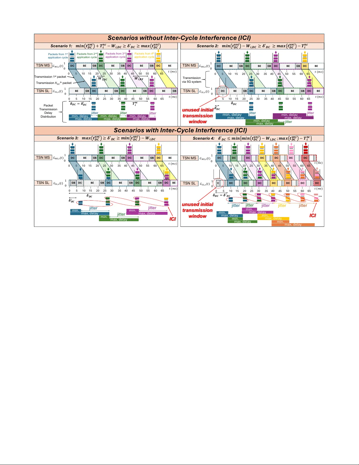
This work is licensed under a Creati ve Commons Attrib ution 4.0 International License. For more information, see creati vecommons.or g. 1 Impact of 5G Latenc y and Jitter on T AS Scheduling in a 5G-TSN Network: An Empirical Study Pablo Rodriguez-Martin , Oscar Adamuz-Hinojosa , Pablo Mu ˜ noz , Julia Caleya-Sanchez , Pablo Ameigeiras Abstract —Deterministic communications are essential to meet the stringent delay and jitter requir ements of Industrial Internet of Things (IIoT) services. IIoT increasingly demands wide-area wireless mobility to support Autonomous Mobile Robots (AMR) and dynamic workﬂows. Integrating Time-Sensitiv e Networking (TSN) with 5G private netw orks is emerging as a promising approach to fulﬁll these requirements. In this architectur e, 5G pro vides wir eless access f or industrial devices, which connect to a TSN backbone that interfaces with the enterprise edge/cloud, where IIoT control and computing systems reside. TSN achieves bounded latency and low jitter using IEEE 802.1Qbv Time- A ware Shaper (T AS), which schedules the network trafﬁc in precise time slots. Howev er , the stochastic delay and jitter inherent in 5G disrupt TSN scheduling, requiring careful tuning of T AS parameters to maintain end-to-end determinism. This paper presents an empirical study evaluating the impact of 5G downlink delay and jitter on T AS scheduling using a testbed with TSN switches and a commercial 5G network. Results show that guaranteeing bounded latency and jitter requir es careful setting of T AS transmission window offset between TSN switches based on the measured 5G delay bounded by a high order p-th percentile. Otherwise, excessive offset may cause additional delay or even a complete loss of determinism. Index T erms —TSN, IEEE 802.1Qbv , 5G, jitter , Industry 4.0, testbed. I . I N T R O D U C T I O N Industrial Internet of Things (IIoT) enables tightly inte- grated Cyber-Physical Systems (CPSs), which are critical for manufacturing automation in modern Industry 4.0. These systems demand deterministic, low-latenc y communication to guarantee safe and predictable operation in dynamic in- dustrial en vironments [1]. Among the most demanding IIoT applications are Connected Robotics and Autonomous Sys- tems (CRAS), including Autonomous Mobile Robots (AMRs), drones, and intelligent agents. These systems rely on precise coordination between sensing, computing, and actuation, and are highly sensitive to communication delays and jitter [2]. T o meet these demands, T ime-Sensitive Networking (TSN) standards deﬁne mechanisms that enable deterministic com- munication over wired Ethernet infrastructures [3]. One of the This work has been ﬁnancially supported by the Ministry for Digital T ransformation and the Civil Service of the Spanish Government through TSI-063000-2021-28 (6G-CHR ONOS) project, and by the European Union through the Recovery , T ransformation and Resilience Plan - NextGenera- tionEU. Additionally , this publication is part of grant PID2022-137329OB- C43 funded by MICIU/AEI/10.13039/501100011033 and ERDF/EU, and part of FPU Grant 21/04225 funded by the Spanish Ministry of Universities. Funding for open access charge: Universidad de Granada / CBUA. The authors are with the Department of Signal Theory , T elemat- ics and Communications; and with the Research Center on Information and Communication T echnologies, both from the Uni versity of Granada, Granada, Spain. E-mails: { pablorodrimar, oadamuz, pabloml, jcaleyas, pameigeiras } @ugr.es . key components of TSN is the IEEE 802.1Qbv T ime-A w are Shaper (T AS), which operates at the output ports of TSN switches. T AS enforces scheduled access to the transmission medium by periodically opening and closing gates that control the e gress of pack ets from dif ferent traf ﬁc queues. By precisely determining when each queue is allowed to transmit, T AS ensures bounded delay and low jitter for selected trafﬁc classes. This deterministic behavior is essential to support time-critical IIoT applications that require guaranteed com- munication performance [4]. Nevertheless, TSN’ s reliance on wired infrastructure limits mobility and ﬂexibility , especially in complex industrial settings. T o overcome these limitations, 5th Generation (5G) mobile networks offer mobility , ﬂexibility , wide-area cov erage, and ultra-Reliable and Low-Latency Communications (uRLLC) capabilities, which hav e spark ed signiﬁcant interest in inte- grating 5G with TSN for industrial scenarios [5]. In this paradigm, industrial end devices such as robots and production line equipment connect wirelessly to the network via the 5G system. The 5G network provides access to a wired TSN back- bone composed of TSN switches connected to edge computing platforms hosting IIoT control functions. This integration aims to combine 5G mobility and coverage with TSN determinism. Howe v er , the stochastic nature of 5G, characterized by v ariable delay in the radio and core segments, disrupts the strict timing required by T AS. This variability challenges the achiev ement of End-to-End (E2E) deterministic communication. T o address these challenges, T AS conﬁgurations must be carefully adapted to maintain synchronized transmissions across TSN switches. In particular , these conﬁgurations must compensate for the delay v ariability introduced by the 5G system while av oiding e xcessiv e b uffering, added latency , or bandwidth inefﬁciencies. Ensuring proper alignment of transmission windows is essential to preserve the deterministic guarantees required by time-sensitiv e IIoT applications. Literature Review . The 5G-TSN integration has drawn substantial research interest. Prior works hav e explored archi- tectures where 5G functions as a logical TSN switch and hav e proposed solutions for time synchronization and Quality of Service (QoS) mapping between domains. Simulation studies hav e also ev aluated T AS scheduling and jitter mitigation; howe v er , these typically rely on idealized wireless models. Although such studies ha ve adv anced the understanding of 5G-TSN integration, critical challenges remain in tuning T AS parameters to compensate for realistic 5G delay and jitter dy- namics. In particular , there is a lack of experimental validation under commercial 5G conditions. For interested readers, a detailed literature revie w is provided in Section VII. 2 Contributions. This article analyzes the impact of 5G- induced delay and jitter on the operation of the IEEE 802.1Qb v T AS in an integrated 5G-TSN network, focusing on the conﬁguration of T AS scheduling parameters to accommodate a delay-critical trafﬁc ﬂow . The main contributions are: C1 W e provide a detailed analysis of the delay components in v olved in the transmission of packets between adjacent T AS-enabled TSN switches interconnected via a 5G net- work. This analysis characterizes ho w 5G-induced delays and jitter interact with T AS parameters, and quantiﬁes their impact on E2E latency performance. C2 Based on this analysis, we identify the conditions under which deterministic communication can be achie ved in 5G-TSN networks. W e thoroughly in vestigate the result- ing scenarios arising from different T AS parameter con- ﬁgurations and provide general conﬁguration guidelines to ensure deterministic behavior . C3 W e implement an experimental testbed integrating a commercial priv ate 5G network and T AS-enabled TSN switches, enabling real-world e valuation of T AS conﬁgu- rations under realistic conditions. The testbed is used to assess the impact of 5G delay and jitter on speciﬁc T AS settings under representative network scenarios. This article builds upon our previous conference work [6], which presented an initial testbed-based study of T AS schedul- ing in integrated 5G-TSN environments. In this extended version, we provide a more comprehensiv e theoretical and experimental analysis of the impact of 5G-induced delay and jitter on T AS operation. W e identify and characterize critical scenarios arising from different T AS parameter conﬁgurations. Furthermore, we deri ve general conﬁguration guidelines and formally establish the conditions required to guarantee deter- ministic E2E performance in 5G-TSN networks. Our results sho w that guaranteeing bounded latency and jitter requires conﬁguring the T AS transmission window offset between TSN switches based on the maximum observed 5G delay , estimated using a high-percentile delay metric. While increasing this offset helps to absorb delay variability , it also increases E2E latency . Moreov er , if the of fset becomes excessi vely large, it may cause misalignment between the transmission windows of TSN switches, thereby violating the deterministic behavior . Additionally , to ensure that packets always arriv e within their assigned transmission windows, the T AS cycle period should be greater than the sum of the peak- to-peak jitter introduced by 5G and the transmission window duration. Finally , we see how additional trafﬁc ﬂows with the same priority may also increase 5G delay and jitter . Similarly , if the 5G network lacks proper isolation between trafﬁc types, ﬂows with lower priority can contribute to latency and jitter degradation. Such cases require recalculating T AS parameters. Paper Outline. The paper is organized as follows: Sec- tion II cov ers background on industrial 5G-TSN networks and T AS. Section III presents the system model. Section IV analyzes 5G delay and jitter impact on T AS. Section V describes the testbed and the experimental setup. Section VI reports performance results. Section VII revie ws related work. Section VIII outlines the key conclusions and future work. I I . B AC K G R OU N D O N I N D U S T R I A L 5 G - T S N N E T W O R K S This section overvie ws 5G-TSN networks in Industry 4.0. First, we introduce the main netw ork segments and k ey charac- teristics of industrial applications. Then, we discuss QoS traf ﬁc management and the T AS mechanism. Finally , we highlight time synchronization for deterministic communications. A. 5G-TSN Network Se gments for Industry Automation As depicted in Fig. 1, three connecti vity segments are deﬁned in a 5G-TSN-based industrial network [5]: • Edge/Cloud Room : Centralizes management tasks han- dled by the Manufacturing Execution System (MES), such as monitoring, data collection, and analytics. Control functions are traditionally performed by Programmable Logic Controllers (PLCs), which may run on dedicated hardware or general-purpose servers, i.e., virtualized PLCs (vPLCs). This layer may also include a network de- vice that provides the TSN Grand Master (GM) clock ref- erence, typically deriv ed from Global Navigation Satellite System (GNSS) [7], for distribution across the network. • 5G System : According to 3rd Generation Partnership Project (3GPP) TS 23.501 (v19.0.0) [8], the 5G system integrates into the TSN netw ork as one or more virtual TSN switches, with the User Plane Functions (UPFs) and User Equipments (UEs) acting as endpoints. The UE connects wirelessly to the next generation Node B (gNB). The TSN T ranslators, speciﬁcally the Network- side Translator (NW -TT) located in the UPF and the Device-side Translator (DS-TT) in the UE, support the integration between the TSN and 5G domains by adapting trafﬁc formats and QoS information, and enabling the transport of synchronization information. • Production Lines : Each includes Field De vices (FDs) such as sensors and actuators, along with local PLCs for distributed control. FDs report operational data to central- ized PLCs, enabling hierarchical decision-making. Each production line connects to a TSN Slav e (SL) switch that receiv es clock signals from the TSN Master (MS) switch via the 5G system and redistributes synchronization to the FDs within this production line. T SN GW … Produ ction li nes gN B 5G Sy ste m NW - TT Edg e/Clou d Room T SN SWI T CH MS PL C … … MES vPL C GM C lo ck T SN Cl ock 5GS Cl ock … Prod uctio n li ne N T SN FD Qo S Flo w #1 UE T SN SWI T CH SL N T AS Qo S Flo w #2 Qo S Flo w #3 No n - T SN FD T SN FD T SN SWI T CH SL 1 T AS Prod uctio n li ne 1 T AS DS - TT UE DS - TT UP F Fig. 1: 5G-TSN network architecture in an Industry 4.0 f actory . 3 B. Industrial applications Industrial network trafﬁc is predominantly delay-sensitive, with E2E latency requirements ranging from hundreds of microseconds to few tens of milliseconds [9]. Although other trafﬁc types exist, such as network control, mobile robotics, and video streams, T AS can be applied to Cyclic-Synchr onous applications, which require highly predictable timing to ensure reliable communications [5], [10]. The Cyclic-Sync hr onous applications consist of periodic communication between devices operating on independent cycles, with synchronization enforced at intermediate network nodes rather than end devices. Each device samples and updates at its own rate, allowing for bounded jitter and some timing variation. Although the E2E packet transmission delay must remain within predictable bounds, occasional variation is tolerated. Thereby , jitter is constrained to the latency bound [10]. This traf ﬁc is commonly used in controller- to-I/O exchanges, periodic sensor polling, and updates to supervisory systems. Examples include PLC-to-actuator re- sponse commands, graphic updates to Supervisory Control and Data Acquisition (SCAD A) systems, and routine diagnostic or historian data transfers. In addition, another category of time-sensitiv e industrial ap- plications coexists with Cyclic-Synchr onous : the Isochr onous . Although both of them require strict delay and jitter analysis in 5G-TSN networks, our work addresses general Cyclic- Synchr onous applications and ev aluates the feasibility of their scheduling, as the stringent requirements of Isoc hr onous ap- plications cannot currently be met, which signiﬁcantly exceed the latency capabilities of existing 5G deployments [11]. C. QoS T raf ﬁc Management T raf ﬁc prioritization in TSN networks relies on the 3- bit Priority Code Point (PCP) ﬁeld deﬁned in IEEE 802.1Q V irtual Local Area Network (VLAN) tags, allowing up to eight priority levels [3]. These levels enable differentiation according to QoS requirements: higher values (i.e., PCP 4–7) are typically assigned to critical trafﬁc, while lower ones (i.e., PCP 0–3) serve less time-sensitive or best-effort data [5]. In 5G networks, QoS is managed for each ﬂow by a QoS Flow ID (QFI) and associated with a standardized 5G QoS Identiﬁer (5QI), as speciﬁed in 3GPP TS 23.501 [8]. Each 5QI deﬁnes key performance characteristics such as priority lev el, delay tolerance, and packet error rate, which determine the treatment of trafﬁc throughout the 5G system [12]. While TSN enforces QoS through PCP-based prioritization, 5G employs 5QI-driven ﬂow control to differentiate trafﬁc. The mapping between TSN trafﬁc classes and 5G QoS ﬂows remains an activ e research topic, primarily due to the semantic differences between the PCP-based prioritization in TSN and the 5QI-based framework in 5G. As shown in [9], a feasible approach in volv es classifying Ethernet frames based on their PCP ﬁeld at the UE and UPF, using packet ﬁlters to associate them with appropriate 5G QoS ﬂows. D. IEEE 802.1Qbv T ime-A war e Shaper (T AS) IEEE 802.1Qbv is a TSN standard that speciﬁes the T AS mechanism, which enables time-aware scheduling of Layer 2 frames at the e gress ports of TSN switches based on QoS requirements [13]–[15]. T AS utilizes the PCP ﬁeld in the IEEE 802.1Q header to classify packets into one of eight First-In First-Out (FIFO) queues. At each egress port, these queues are prioritized to ensure that higher-priority trafﬁc is transmitted before lower -priority trafﬁc. Each egress port is controlled by a Gate Control List (GCL), which deﬁnes a time-triggered transmission schedule divided into transmission windows gov erned by the clock reference. During each transmission windo w , one or more queues are permitted to transmit, depending on the binary state of their associated gates. Each queue has its own gate, and the GCL speciﬁes the time intervals during which each gate is open or closed. When multiple gates are open, transmission order typically follows queue priority , although exact behavior may depend on the switch implementation. T AS scheduling is or ganized around periodic netw ork cycles that enable deterministic communication. A network cycle consists of a ﬁxed-duration time interval which encompasses a full instance of a speciﬁc set of transmission windo ws deﬁned by the GCL [16]. The duration of the network c ycle is typically chosen to align with the application cycles in v olved, which are deﬁned as the periods at which message exchanges occur . This alignment is commonly achie v ed by selecting the netw ork cycle duration as the greatest common divisor of the in volv ed application cycles. For more information on T AS see [4]. E. Synchr onization in 5G-TSN Networks T ime synchronization is essential in 5G-TSN networks to support the deterministic requirements of IIoT applications. In typical TSN architectures, a TSN MS switch distributes the GM clock via Precision Time Protocol (PTP) or generalized Precision Time Protocol (gPTP) messages to multiple TSN SL switches, each deployed along a different production line, as deﬁned in Section II-A. Upon receiving these messages, each TSN SL switch estimates the time difference between its local clock and the reference clock of the TSN MS switch, known as the clock offset, and adjusts its local time accordingly [17]. According to the architecture deﬁned in 3GPP TS 23.501 [8], TSN translators, speciﬁcally the NW -TT and DS- TT, enable propagation of the GM clock across the 5G system to the TSN domain, thus maintaining clock consistency across TSN switches interconnected via 5G (see Fig. 1). A widely adopted conﬁguration for propagating synchronization o ver 5G is the T ransparent Clock (TC) mode deﬁned in IEEE 1588 [18]–[20], where synchronization messages are forwarded with the correctionField updated to reﬂect the residence time within each intermediate node, while original timestamps remain unchanged. Unlike Boundary Clock (BC) mode, where each node terminates and regenerates synchronization mes- sages, TC mode preserves a single timing domain by accumu- lating residence times [21]. The NW -TT and DS-TT measure the residence time within the 5G system and include this delay in the forwarded messages with the correctionField . This operation complies with IEEE 1588-2019 and enables accurate clock correction at the TSN endpoint. For more information see [17]–[21]. 4 Discrepancies in the clocks of dif ferent devices within the 5G-TSN network may occur , prev enting the devices from updating their clocks accurately . The 3GPP TS 22.104 [22] speciﬁes that a maximum clock drift contrib ution of 900 ns must be guaranteed for 5G systems to enable time-critical industrial applications. In line with this, the work in [20] em- pirically quantizes a maximum peak-to-peak synchronization error of 500 ns, which is signiﬁcantly below the requirement. I I I . S Y S T E M M O D E L This section introduces the network and trafﬁc models. W e then describe the T AS model, follo wed by a description of the different sources of latency in the system. T able I provides a summary of key mathematical notations used throughout the paper . Notation Con ventions. W e use calligraphic letters (e.g., X ) to denote sets. Lo wercase letters (e.g., y ) represent random variables, while uppercase letters (e.g., Y ) denote constant parameters. Binary variables are typeset in uppercase sans serif font (e.g., X ). Subscripts indicate that a parameter applies to speciﬁc elements of a gi ven set; for example, z i,j refers to the parameter z corresponding to elements i ∈ I and j ∈ J . Superscripts provide descriptive annotations, e.g., z desc denotes the v ariable z with descriptor ”desc”. In addition, f x ( · ) and F x ( · ) denote the Probability Density Function (PDF) and Cumulati ve Distribution Function (CDF) of the random variable x , respecti vely . Finally , the letter ˆ Z denotes the statistical upper bound of F x ( · ) . A. Network Model W e consider a set of network nodes denoted by I , comprising: ( i ) two TSN switches, denoted as master switch MS and slav e switch SL, respecti vely; ( ii ) two TSN translators, one being a network-side translator and denoted as NW -TT and the other being the device-side translator and denoted as DS-TT; ( iii ) a 5G UE denoted as UE; and ( iv ) a 5G gNB and an UPF, denoted by gNB and UPF, respectiv ely . Each communication link is represented by ε , and the set of all such links is denoted by E . A speciﬁc link between nodes i and j is denoted by ε i,j ∈ E , where i, j ∈ I . The topology is deﬁned by the sequential links: E ≡ { ε MS , NW -TT , ε NW -TT , UPF , ε UPF , gNB , ε gNB , UE , ε UE , DS-TT , ε DS-TT , SL } . W e deﬁne the subset of nodes corresponding to the 5G system as I 5G ≡ { UE , gNB , UPF , NW -TT , DS-TT } . Similarly , the virtual 5G system link set E 5G ⊂ E contains the subset of physical links that connect the nodes of the 5G system, i.e., E 5G ≡ { ε NW -TT , UPF , ε UPF , gNB , ε gNB , UE , ε UE , DS-TT } . Finally , we deﬁne the subset of TSN switches as I TSN ⊂ I , i.e., I TSN ≡ { MS , SL } , which are interconnected via the 5G system with the link set E TSN ⊂ E , containing the subset of physical links to the 5G bridge bounds NW -TT and DS-TT, i.e., E TSN ≡ { ε MS,NW -TT , ε DS-TT,SL } , respectiv ely . B. T r afﬁc Model and QoS Level Assignment Let S denote the set of traf ﬁc ﬂo ws traversing the considered 5G-TSN network. Speciﬁcally , S includes: • A downlink Delay-Critical (DC) ﬂow generated by a Cyclic-Sync hr onous application, as described in Sec- tion II-B. W e assume a DC ﬂow in downlink as a set of packets sharing a source at the Edge/Cloud Room, e.g., a PLC, and an y of the de vices in the same production line as the destination, e.g., actuators, which are typically served by a common switch, i.e., the SL switch. Each application cycle , of periodic duration T app DC , the PLC generates a batch of N DC packets of constant size L DC , re- sulting in an av erage data rate R gen DC = N DC · L DC /T app DC , as a response delivered to all these actuators after pro- cessing the production state [23]. Additionally , packets must trav erse the 5G-TSN network subject to an E2E delay constraint d E2E DC ≤ D DC . Assuming these packets belong to a single application, they share the same timing constraints between them. • A downlink Best-Effort (BE) ﬂo w composed of packets that do not require strict timing guarantees. W e assume packets of constant size L BE are generated at a constant data rate R gen BE . • Uplink and do wnlink PTP ﬂo ws are considered to support clock synchronization among TSN switches. The exchange of these messages, as deﬁned by the PTP standard, occurs periodically , with an application cycle T app PTP signiﬁcantly larger than T app DC , i.e., T app PTP ≫ T app DC . PTP ﬂo ws are assigned the highest priority , followed by DC and then BE ﬂows, consistently across both the 5G and TSN domains. Accordingly , PTP and DC packets are assigned higher PCP values for TSN scheduling, and they are mapped to 5G QoS ﬂo ws with lower 5QI indices, indicating stricter QoS treatment. BE packets are mapped to the lowest priority class with higher 5QI index. C. T AS model At each TSN switch i ∈ I TSN , each egress port is associated with a set Q i containing up to eight output queues. W e assume a one-to-one mapping between each queue q ∈ Q i and a trafﬁc ﬂow s ∈ S , allowing interchangeability of q and s throughout this paper . Furthermore, we assume the GCL enforces mutually exclusiv e g ate openings among the eight queues per egress port, guaranteeing that only one queue is permitted to transmit at any giv en instant. Accordingly , the GCL conﬁguration for queue q ∈ Q i at switch i ∈ I TSN is formally expressed by Eq. (1). The binary variable G i,q ( t ) indicates whether the gate is open (1) or closed (0). The gates operate periodically with period T nc i , referred to as the network cycle . In the network cycle n = 0 , the gate opening and closing instants, T open i,q and T closed i,q , deﬁne the transmission window duration W i,q = T closed i,q − T open i,q . G i,q ( t ) =      1 , nT nc i + T open i,q < t ≤ nT nc i + T closed i,q , ∀ n ∈ N ∪ { 0 } . 0 , otherwise . (1) The DC ﬂo w period T app DC typically ranges from sev eral hundreds of microseconds up to a few tens of milliseconds, whereas PTP synchronization messages are generated approx- imately every T app PTP ≈ 1 s. Giv en that condition T app PTP ≫ T app DC , 5 T ABLE I: Main Mathematical Notations V ariable Description V ariable Description I Set of network nodes. E Set of links. ε i,j Link ε between network nodes i and j , ∀ i, j ∈ I . I 5G Subset of 5G network nodes. E 5G Subset of links within the 5G system. I TSN Subset of TSN nodes. E TSN Subset of links within the TSN system. S Set of trafﬁc ﬂows. s Traf ﬁc ﬂow type s ∈ S . T app s Application cycle for trafﬁc ﬂow s ∈ S . N s Packets generated in an application cycle for trafﬁc ﬂow s ∈ S . L s Packet size for trafﬁc ﬂow s ∈ S . R gen s Data rate for trafﬁc ﬂow s ∈ S . d E2E s E2E packet transmission delay for trafﬁc ﬂow s ∈ S . D s Delay bound for E2E transmission time for trafﬁc ﬂow s ∈ S . Q i Set of queues in an output port in node i ∈ I TSN . q Output port queue q ∈ Q i . G i,q ( t ) Binary function to open/close the gate for queue q ∈ Q i at node i ∈ I TSN . T nc i Network cycle in node i ∈ I TSN . T open i,q Time instant the gate is open for queue q ∈ Q i in node i ∈ I TSN . T closed i,q Time instant the gate is closed for queue q ∈ Q i in node i ∈ I TSN . W i,s T ransmission windows in node i ∈ I TSN for trafﬁc ﬂow s ∈ S . T GB Duration of the guard band. d que,in i Packet waiting time in the input queue in node i ∈ I . d proc i Packet processing time in node i ∈ I . d que,out i,q Packet waiting time in the output queue q ∈ Q i in node i ∈ I . d tran ε i,j ,s Packet transmission time at link ε i,j ∈ E for trafﬁc ﬂow s ∈ S . r ε i,j Data rate at link ε i,j ∈ E . D prop ε i,j Propagation time in the physical medium of link ε i,j ∈ E . d 5G s Packet transmission time within the 5G system for trafﬁc ﬂow s ∈ S . d MS,SL s Packet delay between MS and SL output ports for trafﬁc ﬂow s ∈ S . e d MS,SL s Packet delay from MS output port to SL processing for trafﬁc ﬂow s ∈ S . ∆ i,j Synchronization error between TSN nodes i, j ∈ I TSN . d emp s Empirical delay measured in our study for trafﬁc ﬂow s ∈ S . e d emp s ZWSL empirical delay measured in our study for trafﬁc ﬂow s ∈ S . δ s Offset between two adjacent TSN switches for trafﬁc ﬂow s ∈ S . ˆ D emp s,p Percentile p of the ZWSL empirical delay distribution for trafﬁc ﬂow s ∈ S . δ ′ s Network cycle offset for trafﬁc ﬂow s ∈ S . t uni s Uncertainty interval for trafﬁc ﬂow s ∈ S . t jit s 5G-TSN network jitter for trafﬁc ﬂow s ∈ S . we consider the duration of the network cycle , T nc i = T app DC , ∀ i ∈ I TSN , as the DC ﬂow is the primary target of this work. Each network cycle comprises three non-overlapping trans- mission windows (see Fig. 2): W i, DC for the DC trafﬁc, W i, PTP for PTP synchronization messages and W i, BE for BE trafﬁc, followed by a ﬁxed guard band T GB to av oid interference on DC traf ﬁc. Thus, T nc i = W i, DC + W i, PTP + W i, BE + T GB , ∀ i ∈ I TSN . W e consider W i, PTP occupies a negligible fraction of T nc i , 100 to 1000 times smaller , due to the low frequency of synchronization messages, i.e., W i, PTP ≪ W i, DC and W i, PTP ≪ W i, BE . Due to this and for ease of reading, W i, PTP is omitted in subsequent equations, while it is implicitly assumed to be scheduled immediately after W i, DC . For further details on PTP planning, see [21]. Finally , at the MS, each batch of N DC packets belonging to the DC ﬂo w is assumed to be av ailable at the start of ev ery network cycle . D. Delay Model For each packet of ﬂow s ∈ S tra versing node i ∈ I , the total delay comprises ﬁv e components: input queuing delay , processing delay , output queuing delay , transmission delay , and propagation delay . These can be seen in Fig. 3. The input queuing delay d que,in i,s is the interv al between the arriv al of a packet at node i and the start of its processing. The processing delay d proc i,s corresponds to the time required by node i to parse the packet header and determine the forwarding action. The output queuing delay d que,out i,s refers to the delay T S N d e v i c e i , p or t p DC BE W i,BE n et w o r k c y c l e n n e tw o r k cy cl e n + 1 n e tw o r k cy cl e n – 1 T GB DC BE t PT P G B T nc W i,P T P W i,D C i G B Fig. 2: Diagram of T AS-scheduled network cycles in GCL. from the end of processing at node i until the packet is transmitted to the next hop. The transmission delay d tran ε i,j ,s corresponds to the time needed to serialize all bits of the packet over the link ε i,j ∈ E . It depends on the packet size L s and the link capacity r ε i,j , and is giv en by d tran ε i,j ,s = L s /r ε i,j . The propagation delay D prop ε i,j is the time a signal takes to trav el through link ε i,j ∈ E and is assumed to be constant for any ﬂow s ∈ S in that link in time. I V . A NA LY S I S O F 5 G D E L A Y A N D J I T T E R O N T A S S C H E D U L I N G In this section, we analyze how 5G impacts T AS scheduling performance. First, we deﬁne the E2E delay for a packet of an arbitrary ﬂow and study how the 5G delay component impacts it. Then, we formalize the constraint for the transmission window of the DC ﬂow in TSN switches. Next, we introduce the concept of offset between the network cycles of the MS and SL switches, and derive the conditions required to ensure deterministic communication. Finally , we analyze ho w this offset interacts with the 5G delay component, and ev aluate how dif ferent T AS parameter conﬁgurations inﬂuence the scheduling performance across various scenarios. A. Analysis of Delay Components The set of ﬂows S traverses a sequence of network nodes to reach their destination, as illustrated in Fig. 3. The E2E packet transmission delay d E2E s for the ﬂow s ∈ S along this path is computed as the sum of delays at each network node plus the transmission delays on each link: d E2E s = X i ∈I  d que,in i,s + d proc i,s + d que,out i,s  + X e ∈E  d tran e,s + D prop e  . (2) The 5G delay d 5G s is deﬁned as the sum of node processing and queuing delays, plus link transmission in the 5G domain: d 5G s = X j ∈I 5G  d que,in j,s + d proc j,s + d que,out j,s  + X k ∈E 5G  d tran k,s + D prop k  . (3) 6 TSN MS UE gN B TSN SL DS - TT NW - TT                                                                                            UPF DC PTP BE DC PTP BE    ~ Fig. 3: 5G-TSN network elements and associated delay terms in the downlink transmission for each trafﬁc ﬂow s ∈ S . T o assess the impact of 5G in combination with the T AS scheduling, we consider the packet delay between the MS and SL output ports, d MS,SL s , and compute it as follows: d MS,SL s = X ε ⊂E TSN  d tran ε,s + D prop ε  + d 5G s + d que,in SL ,s + d proc SL + d que,out SL ,s . (4) For con venience, we also consider the packet delay between the MS output port and the SL switch processing, e d MS,SL s , that is, excluding the SL output queuing delay , d que,out SL ,s , as it is inﬂuenced by the T AS conﬁguration: e d MS,SL s = X ε ⊂E TSN  d tran ε,s + D prop ε  + d 5G s + d que,in SL ,s + d proc SL . (5) In this work, we rely on empirical delay measurements for our analysis. Therefore, our model has to consider the synchro- nization error that inherently affects the delay measurement between separate TSN nodes, i.e., ∆ i,j , ∀ i, j ∈ I TSN . Hence, the empirical measurement of the packet delay between the MS and the SL output ports, d emp s , could be expressed as in Eq. (6), where ∆ MS,SL refers to the synchronization error between MS and SL. d emp s = d MS,SL s + ∆ MS,SL . (6) The value of ∆ MS,SL is assumed to take positiv e or negati v e values, as clocks may be ahead or behind each other at any instant. A higher | ∆ MS,SL | may cause the measurements to become unreliable, as it distorts the temporal correspondence between events. In this way , the E2E latency from Eq. (2) is also affected by the synchronization error . Thus, its empirical measurements can be written as d E2Emp s in Eq. (7). d E2Emp s = d que,in MS ,s + d proc MS + d que,out MS ,s + d emp s . (7) Similarly , the empirical measurement of the packet delay between the MS output port and the SL switch processing, from now on Zero-W ait-at-SL (ZWSL) empirical delay , e d emp s , could be expressed as in Eq. (8). e d emp s = e d MS,SL s + ∆ MS,SL . (8) Observation –. The 5G system delay , d 5G s , is signiﬁcantly larger than the transmission delays ov er wired links, d tran ε i,j ,s , ∀ ε i,j ∈ E \{ ε gNB,UE } , ∀ i, j ∈ I ; the propagation delays, D prop ε i,j , ∀ ε i,j ∈ E , ∀ i, j ∈ I ; and processing delays in the TSN switches, d proc i,s , ∀ i ∈ I TSN . On the one hand, transmission delays over wired links are typically within the microsecond range. For example, a 200 Bytes packet, assuming 42 Bytes of ov erhead, has a transmission delay of 1.9 µ s in 1 Gbps links. Similarly , processing delays in TSN switches are typically also in the microsecond range [24]. On the other hand, 5G system delay is in the range from milliseconds to a few tens of milliseconds [11]. This delay and jitter dominance will be corroborated experimentally in Section VI. As a consequence of this observation, the 5G system delay , and its associated jitter, play a prominent role in Eq. (4)-(8), and therefore in the T AS conﬁguration of the TSN switches. Since our analysis targets the DC ﬂow , the formulation presented from this point onward assumes s = DC. B. T r ansmission W indow Size in T AS Scheduling The transmission window duration W i, DC for ﬂow DC ∈ S at TSN switch i ∈ I TSN must satisfy two conditions: it must be strictly shorter than the network cycle T nc i and equal or greater than the cumulativ e transmission time of N DC packets through the output port. These constraints are formalized in Eq. (9), where j ∈ I is the next network node after switch i . N DC · d tran ε i,j , DC ≤ W i, DC < T nc i . (9) V iolating these bounds can lead to performance degradation. If W i, DC is too short, not all N DC packets can be transmitted within a single network cycle . The remaining packets accumu- late and are deferred to subsequent network cycles , introducing additional delays that are multiples of T nc i . On the other hand, if W i, DC exceeds the network cycle duration, it monopolizes the schedule, prev enting other ﬂows s ∈ S \ { DC } from being scheduled during that network cycle . C. T AS Scheduling Offset between TSN Switches W e consider identical T AS scheduling conﬁgurations at both MS and SL switches, i.e., T nc MS = T nc SL and W MS , DC = W SL , DC . Under this assumption, let us deﬁne the offset δ DC as the time difference between the start of the network cycle at the MS and SL. This offset must be conﬁgured to ensure all N DC packets, generated within a single application cycle , arrive at the output queue of the SL and are transmitted through its egress port before the corresponding transmission window closes. Since all N DC packets are sent as a b urst from the MS into the 5G system, it is essential to characterize the delay experienced by these packets in the 5G system to establish a value for the offset δ DC . Assuming that the 5G system capacity is generally lower than the capacity of a wired link [11], the 7 5G segment constitutes a bottleneck in the 5G-TSN network, where packets experience increasing queuing delays. The ﬁrst packet in the burst, if no retransmission is required, may trav erse the 5G network with minimal delay , i.e., min( d 5G DC ) , while each subsequent packet must wait for the transmission of the previous packets. Consequently , delay accumulates across the b urst, such that the last packet tends to experience the highest latency , i.e., max( d 5G DC ) , which already includes the cumulativ e queuing delay of the entire burst. Consequently , the offset δ DC must be set to at least max ( e d emp DC ) to guarantee the a vailability of packets at the SL output port queue to be transmitted on time. This leads to the condition in Eq. (10). δ DC ≥ max ( e d emp DC ) . (10) Since e d emp DC is random by nature, it is necessary to character- ize its beha vior statistically . In this work, we deﬁne a statistical upper bound based on a given percentile p ∈ [0 , 1) of the CDF F e d emp DC ( · ) of the ZWSL empirical delay . Speciﬁcally , we denote this bound as ˆ D emp DC ,p = F − 1 e d emp DC ( p ) , which corresponds to the p -th percentile of the delay distribution. A higher value of p increases the conﬁdence e d emp DC will remain belo w ˆ D emp DC ,p [25]. For instance, setting p = 0 . 999 yields an upper bound such that 99.9% of packets experience delays below this value. Accordingly , we set the offset δ DC as in Eq. (11), ensuring that at least p · 100 % of packets have been queued before the transmission window in the SL closes. δ DC ≥ ˆ D emp DC,p . (11) An additional parameter of interest is the time instant at which an initial transmission window opens at the SL for transmitting packets of the DC ﬂo w . W e denote this instant as the network cycle offset δ ′ DC , formally deﬁned as follows: δ ′ DC = ( δ DC , if δ DC < T nc i . δ DC mo d T nc i , otherwise . (12) The network cycle offset δ ′ DC depends on the conﬁgured of f- set δ DC and the network cycle duration T nc i . When δ DC < T nc i , it holds that δ ′ DC = δ DC , and the transmission window opens exactly at the conﬁgured of fset . Con versely , if δ DC ≥ T nc i , the initial transmission opportunity may occur before the conﬁgured offset , and the effecti v e opening time is given by δ ′ DC = δ DC mo d T nc i ∈ [0 , T nc i ) . D. Conditions for Determinism under 5G Delay and Jitter W e consider deterministic transmission as the scenario in which the entire b urst of N DC packets in the same tr ansmission window of a given network cycle at the MS are delivered and forwarded within a single transmission window at the SL switch. In this case, the E2E jitter remains bounded by the window size W i, DC , thus enabling predictable communication. T o determine if a deterministic transmission is possible, it is essential to examine the relationship between the 5G-induced delay and jitter and the following T AS parameters: (i) the network cycle offset δ ′ DC , (ii) the network cycle duration T nc i , and (iii) the size of the transmission window W i, DC . Let us deﬁne the uncertainty interval t uni DC as the range of possible delays a packet from DC ﬂow may experience when trav ersing the 5G-TSN network: t uni DC = h min( e d emp DC ) , ˆ D emp DC ,p i . (13) This interval is bounded by the minimum and maximum values of the per-packet e d emp DC . Note that we consider the p -th percentile of the ZWSL empirical delay distrib ution as the maximum value of the uncertainty interval . Accordingly , we deﬁne the induced jitter of the 5G-TSN network, t jit DC , as the difference between the limits of the uncertainty interval: t jit DC = max( t uni DC ) − min( t uni DC ) . (14) T o guarantee a deterministic transmission , two timing con- ditions must be satisﬁed between MS and SL: F irst Condition for Determinism: T o ensure this one-to- one correspondence between the transmission windows at MS and SL, the start time of the transmission window at the SL switch, i.e., δ ′ DC , must satisfy the two boundary conditions valid for any network cycle in Eq. (15) or, alternati vely , those in Eq. (16). C1: max  t uni DC  ≤ δ ′ DC , C2: δ ′ DC + W i, DC ≤ min  t uni DC  + T nc i . (15) The condition C1 indicates that the transmission window at the SL switch must start only after the last pack et of the burst transmitted by the MS switch has arriv ed in the current network cycle , ensuring that all those packets are already av ailable when the window opens. The condition C2 requires that the transmission window must close before the ﬁrst packet served in a subsequent network cycle at the MS switch arrives at the SL switch in the next network cycle . C3: max  t uni DC  ≤ δ ′ DC + T nc i , C4: δ ′ DC + W i, DC ≤ min  t uni DC  . (16) The condition C3 stipulates that the transmission window at the SL switch can start only after the last packet of the burst transmitted by the MS switch has arri ved in the previous network cycle . The condition C4 designates that the transmission window must close before the ﬁrst packet served in a subsequent network cycle at the MS switch arriv es at the SL switch in the current network cycle . Either Eq. (15) or Eq. (16) ensures that all N DC packets can be forwarded within a single transmission window . Otherwise, the burst will necessarily be split across multiple transmission windows , violating the determinism requirement. W e call this effect Inter-Cycle Interference (ICI), where the packets sched- uled in a network cycle may interfere with the ones scheduled in the next network cycle . As max  t uni DC  = ˆ D emp DC ,p , in Eq. (15) and Eq. (16) the transmission window forwarding all N DC packets at the SL switch is lower bounded by the p -th percentile of the delay distribution of the ZWSL empirical delay , e d emp DC , and hence by the p -th percentile of 5G system delay distribution. As a relev ant consequence, the packet empirical delay d emp DC may increase in exchange for achieving deterministic transmission according to the p -th percentile and the network cycle duration. 8 j i tte r j i tte r S c e na r io 4 :                  ,  ;           S c e na r io 1 :        +       ,                DC DC DC DC BE 0 5 10 15 20 25 30 35 40 45 50 55 60 65  (  ) DC DC DC 0 5 10 15 20 25 30 35 40 45 50 55 60 65  (  ) BE BE BE BE BE BE GB GB GB GB GB GB 1 0 1 0 T SN M S T r a n s mi s s io n 1 s t pac k et T r a n s mi s s io n   t h pac k et   ,      ,     =   󰆒 Pa cke t s f ro m 1 st appl i c at i on c y c l e Pa cke t s f ro m 2 nd appl i c at i on c y c l e Pa cke t s f ro m 3 rd appl i c at i on c y c l e Pa cke t s f ro m 4 th appl i c at i on c y c l e T SN SL j i tte r GB BE j i tte r j i tte r   ,  S c e na r io 2 :           ,                   DC DC DC DC BE 0 5 10 15 20 25 30 35 40 45 50 55 60 65  (  ) DC DC DC 0 5 10 15 20 25 30 35 40 45 50 55 60 65  (  ) BE BE BE BE BE BE GB GB GB GB GB GB 1 0 1 0 T SN M S   ,      ,   T SN SL DC BE … … … … … … … … … … … Sce na r io s w ith o u t I nt e r - C y c l e In t er f er en c e ( IC I) S c e na r io 3 :                        ,   m i n. de l ay m ax . de l ay m i n. de l ay m ax . de l ay m i n. de l ay m ax . de l ay Pa c k e t T r a n s mi s s i o n D el ay D is t r i b u t i o n   j i tte r … … … m i n . d e la y m ax . de l ay m i n. de l ay m ax . de l ay m i n. de l ay m ax . de l ay   󰆒 Sce na r io s w ith I nt e r - C y c l e In t er f er en c e ( IC I) DC DC DC DC BE 0 5 10 15 20 25 30 35 40 45 50 55 60 65  (  ) DC DC DC 0 5 10 15 20 25 30 35 40 45 50 55 60 65  (  ) BE BE BE BE BE BE GB GB GB GB GB GB 1 0 1 0 T SN M S   ,      ,   T SN SL DC BE … … … … GB     󰆒 … … … jitte r IC I jitte r … … … m i n. m ax . de l ay m i n. m ax . de l ay m i n. m ax . de l ay jitte r u n u s e d i n i ti a l tra n s m i s s i o n w i n d o w DC DC DC DC DC DC DC 0 5 10 15 20 25 30 35 40 45 50 55 60 65  (  ) C 0 5 10 15 20 25 30 35 40 45 50 55 60 65  (  ) 1 0 0 T SN M S T r a n s mi s s io n v i a 5G s y s t em   ,      ,   T SN SL 1 … … … … … … … … … … … … DC DC DC DC DC DC DC   =   jitte r IC I jitte r jitte r jitte r … … … … … m i n. m ax . de l ay m i n. m ax . de l ay m i n. m ax . de l ay m i n. m ax . de l ay m i n. m ax . de l ay … … … … … … jitte r   ,     … … u n u s e d i n i ti a l tra n s m i s s i o n w i n d o w Fig. 4: Impact of the 5G delay ov er T AS cycles. All Scenarios: max  t uni DC  = 15 ms, min  t uni DC  = 7 . 5 ms and W i, DC = 5 ms ∀ i ∈ I TSN . Scenario 1: T nc i = 20 ms ∀ i ∈ I TSN and δ DC = 15 ms. Scenario 2: T nc i = 20 ms ∀ i ∈ I TSN and δ DC = 22 . 5 ms. Scenario 3: T nc i = 20 ms ∀ i ∈ I TSN and δ DC = 25 ms. Scenario 4: T nc i = 10 ms ∀ i ∈ I TSN and δ DC = 7 . 5 ms. Second Condition for Determinism: Directly comparing the upper and lower bounds for δ ′ DC isolated on one side of each of the inequalities, either in Eq. (15) or Eq. (16), leads to the additional condition in Eq. (17), which relates ho w the T AS parameters must be conﬁgured with respect to the 5G jitter to guarantee deterministic transmission . T nc i − W i, DC ≥ t jit DC . (17) Eq. (17) imposes a second fundamental condition on the interplay between the T AS conﬁguration and the statistical behavior of the 5G system. It establishes that the 5G-induced jitter imposes a lower bound on the network cycle T nc i . Additionally , increasing the transmission window W i, DC not only requires larger network cycle T nc i as Eq. (17) shows, b ut it will also indirectly increase t jit DC due to the cumulativ e queuing effect on pack ets in the 5G system. Furthermore, Eq. (17) also imposes a limit on the link utilization for DC trafﬁc, as additional transmission windows of DC trafﬁc in the network cycle period would cause ICI and break the determinism. The conditions deri ved above pro vide a foundation for deterministic transmission . In the following subsection, we perform a detailed analysis of these conditions under different parameter conﬁgurations, identifying scenarios in which deter- minism is either achie ved or violated to later be experimentally demonstrated in Section VI. E. Impact of 5G Delay on Offset Conﬁguration The analysis of the impact of the empirical delay d emp DC , largely dominated by the 5G system, on the coordinated operation of T AS mechanism in both the MS and SL switches is illustrated in Fig. 4, which sho ws the timing of data transmissions through the egress ports of the MS and SL switches interconnected via a 5G system. Each timeline is structured into consecutiv e network cycles , each of which contains a single transmission window allocated to the DC ﬂow . The ﬁgure considers four distinct scenarios based on the relativ e timing between the transmission windows at the SL and the uncertainty interval t uni DC in Eq. (13). These scenarios are deﬁned by speciﬁc conditions on the network parameters T nc i , W i, DC , and the conﬁgured offset δ DC , which implicitly determines δ ′ DC according to Eq. (12). Scenario 1: Deterministic transmission with early arrival. min( t uni DC ) + T nc i − W i, DC ≥ δ ′ DC ≥ max( t uni DC ) . (18) From the previous conditions C1 and C2 in Eq. (15), the lower bound δ ′ DC ≥ max  t uni DC  , and the upper bound, δ ′ DC ≤ min  t uni DC  + T nc i − W i, DC , can be yielded for δ ′ DC in Eq. (18). W ith this, all pack ets from a giv en network cycle arriv e at the SL before the initial transmission window 9 opens. As a result, they can be transmitted entirely within that transmission window . This conﬁguration ensures deterministic behavior in the 5G-TSN network, with packet jitter bounded by the duration of the transmission window , W i, DC . Scenario 2: Deterministic transmission with unused initial transmission window . min( t uni DC ) − W i, DC ≥ δ ′ DC ≥ max( t uni DC ) − T nc i . (19) Now , from conditions C3 and C4 in Eq. (16), the lower bound δ ′ DC ≥ max  t uni DC  − T nc i , and the upper bound, δ ′ DC ≤ min  t uni DC  − W i, DC , can be yielded for δ ′ DC in Eq. (19). No packets arrive before the initial transmission window at SL closes, which therefore remains unused. Howe ver , all packets are av ailable before the second transmission window opens, allowing their complete transmission. This results in higher minimum and maximum packet transmission delays compared to Scenario 1 , increased by the waiting in the queue until the next network cycle . Nev ertheless, the transmission remains deterministic, with bounded jitter . Scenario 3: Non-deterministic transmission with partial packet arrival. max( t uni DC ) ≥ δ ′ DC ≥ min( t uni DC ) − W i, DC . (20) Some packets arrive in time to be transmitted during the initial transmission window at the SL, while others must wait for the second transmission window . This results in ICI, as deﬁned in Section IV -D. Consequently , jitter increases to at least one full network cycle , thereby affecting packets scheduled in the next network cycle , and determinism is lost in the 5G-TSN network. Scenario 4: Non-deterministic transmission with delayed arrival. δ ′ DC ≤ min  min( t uni DC ) − W i, DC , max( t uni DC ) − T nc i  . (21) This conﬁguration represents the most adverse condition for the 5G-TSN network because Eq. (17) is not met. This means ICI is unav oidable. In this case, the second or subsequent transmission windows at SL may close before all packets hav e arri ved, so some packets may be transmitted in the next network cycle , leading to the highest delays and jitter among all scenarios. W e reﬂect the case where ICI is extended to a third transmission window due to the accumulation of packets at the SL’ s buf fer between network cycles . V . T E S T B E D A N D E X P E R I M E N T A L S E T U P In this section, we describe the implemented 5G-TSN testbed and the considered experimental setup. A. T estbed Description T o carry out our empirical analysis, we implemented the testbed depicted in Fig. 5. Its components are described belo w . 5G System. The 5G network comprises a single gNB and a 5G core, both implemented on a PC with a 50 MHz PCIe Amarisoft Software Deﬁned Radio (SDR) cards and an AMARI NW 600 license. The gNB operates in the n78 band with 30 kHz subcarrier spacing and a bandwidth of 50 MHz. Data transmission uses a Time Division Duplex (TDD) scheme with a pattern of four consecutiv e downlink slots, four uplink slots, and two ﬂexible slots. Although our analysis focuses solely on downlink trafﬁc, this conﬁguration reserves resources for uplink, enabling a realistic testbed en vironment [26]. T wo UEs are deployed, each consisting of a Quectel RM500Q-GL modem connected via USB to an Intel NUC 10 (i7-10710U, 16 GB RAM, 512 GB SSD) running Ubuntu 22.04. Experiments are conducted using one LABIFIX Faraday cage, with gNB antennas connected to the SDR via SMA connectors. Finally , although it is common to assign one DS-TT per UE [5], this proof of concept simpliﬁes the setup by using a single DS-TT for both UEs. Similarly , we use a single NW -TT for simplicity’ s sake. TSN Network. The TSN netw ork is built using Safran’ s WR-Z16 switches. One switch operates as the MS, another as the SL, and two additional switches act as TSN translators, i.e., NW -TT and DS-TT. The MS is directly connected to a Safran SecureSync 2400 server , which provides the GM clock to the SL for time synchronization. Since the 5G system operates in PTP TC mode (implemented in TSN translators [20]), an auxiliary WR-Z16 switch, also synchronized via a second SecureSync 2400, is used to distribute the 5G GM clock between the TSN translators. Each WR-Z16 switch is based on a Xilinx Zynq-7000 FPGA and a 1 GHz dual-core ARM Cortex-A9, enabling high switching rates and low processing delays under a Linux-based OS. The switches support IEEE 802.1Qbv T AS and VLANs, and include sixteen 1GbE Small Form-factor Pluggable (SFP) timing ports conﬁgurable as PTP MS or SL. Each egress port provides four priority hardware queues to separate the different trafﬁc ﬂows, with a maximum buf fer size of 6.6 kB per queue. This limits the number of PCPs from 0 to 3, and also imposes a constraint on sustained throughput, as exceeding the draining capacity leads to packet drops. Additionally , timestamping probes on each port enables high-precision latency measurements between the output ports of the TSN nodes. T estbed Clock Synchronization. Time synchronization be- tween the TSN GM clock server and the MS is established via coaxial cables carrying two signals: a Pulse Per Second (PPS) pulse for absolute phase alignment and a 10 MHz reference for frequency synchronization through oscillator disciplining. Similarly , the auxiliary WR-Z16 switch is synchronized with the 5G GM clock server using the same coaxial interface, enabling accurate time distribution between the NW -TT and DS-TT to enable the TC mode [20]. In the testbed, the MS and SL communicate PTP packets ov er IPv4 using unicast User Datagram Protocol (UDP) and the E2E delay measure- ment mechanism. The PTP transmission rate is conﬁgured to 1 packet per second. End Devices and T estbed Connections. T wo Ubuntu 22.04 L TS servers operate as packet generator with packETH tool and sink, respectively . All components in the testbed are interconnected using 1 Gbps optical ﬁber links, except for the connections between the NW -TT-gNB, and DS-TT-UEs, which use 1 Gbps RJ-45 Ethernet cables. 10 TSN MS Swi tch WR-Z16 au x Optical Fiber RJ45 cables PPS coaxial cables 10 MHz coaxial cables 5G System Faraday's Cage gNB + 5G Core DS-TT Rx server TSN System Edge/Cloud NW -TT Measurement Point Production Lines NUC UE 1 Quectel NUC UE 2 Quectel TSN GM Tx server 5G GM TSN SL Fig. 5: Proof of concept equipment and ev aluated 5G-TSN network scenario. Network T rafﬁc. At the 5G core network, two distinct Data Network Names (DNNs) are conﬁgured to create separate network slices for industrial trafﬁc management. One carries both PTP and DC ﬂows, while the other handles BE ﬂo w , enabling dif ferentiated routing and resource allocation. The 5G network employs IP transport because the considered UE operates without Ethernet-based sessions. T o support Layer 2 industrial automation trafﬁc over IP , a V irtual Extensible LAN (VxLAN)-based tunneling mechanism is implemented [9], with two VxLANs conﬁgured accordingly: one transporting DC and PTP ﬂows, and the other BE ﬂo w . Packets are tagged with PCP values reﬂecting the relativ e priority among the ﬂows: PCP 3 for packets of the PTP ﬂow , PCP 2 for DC ﬂow packets, and PCP 0 for BE ﬂow packets. Additionally , within the 5G network, 5QI values are assigned per ﬂow’ s packets, with 80 for PTP and DC trafﬁc, and 9 for BE trafﬁc. B. Description of Experiments W e ev aluate the packet transmission delay d emp DC for the DC ﬂow across ﬁv e e xperimental scenarios. Each scenario analyzes a speciﬁc T AS conﬁguration parameter to e valuate its effect on the TSN system’ s ability to tolerate 5G-induced delay . Experiment 1: Delay Analysis of 5G Network. W e analyze the effect of varying the traf ﬁc generation rate R gen DC on the delay and jitter of the 5G network to determine ˆ D emp DC ,p and, with it, the uncertainty interval t uni DC . For that, we sweep R gen DC in 300 kbps increments from 350 kbps to 1.55 Mbps. For each R gen DC , the transmission window W MS , DC is calculated based on the lower bound deﬁned in Eq. (9), ensuring compliance with the WR-Z16’ s b uf fer size limitation. This results in transmission windows at MS ranging from 10.5 µ s to 46.5 µ s. T AS is enabled at the MS, while at SL the output queue gate remains open 100% of the time. This is done this way to estimate the ZWSL empirical delay , e d emp DC . The network cycle is ﬁxed at T nc MS = 30 ms. Experiment 2: Delay Analysis based on Offset between transmission windows of MS and SL Switches . W e analyze the effect on d emp DC of different temporal shifts between network cycles at MS and SL. T AS is similarly conﬁgured at both switches, with ﬁxed transmission window W i, DC = 46 . 5 µ s and network cycle T nc i = 30 ms, ∀ i ∈ I TSN . W e sweep offset δ DC = { 5 , 10 , 15 , 20 , 25 , 30 } ms. Experiment 3: Delay Analysis Based on Network Cycle . W e study the inﬂuence of the network cycle on d emp DC with a constant δ DC to analyze the scenarios described in Section IV -E. The network cycle is varied in the range of T nc i = { 6 , 8 , 10 , 12 . 5 , 15 , 17 . 5 , 20 , 22 . 5 } ms ∀ i ∈ I TSN . T r ansmission windows are set to W i, DC = { 9 , 12 , 15 , 18 , 22 . 5 , 25 . 5 , 30 , 33 } µ s, ∀ i ∈ I TSN , respectiv ely , to keep the injected data rate into the 5G-TSN network constant at 1.55 Mbps. Experiment 4: Delay Analysis considering Multiple T raf ﬁc ﬂows with Same-Priority . W e ev aluate the packet transmission delay when multiple distinct ﬂo ws share the same priority output queue. Firstly , T AS is enabled exclusiv ely at the MS, while at the SL, the output queue gate remains open 100% of the time, as in Experiment 1 to obtain e d emp DC . The network cycle is ﬁxed at T nc i = 30 ms ∀ i ∈ I TSN and, to accommodate all the ﬂows, transmission windows are set to W MS , DC = { 0 . 25 , 0 . 5 , 0 . 75 , 1 , 1 . 25 , 1 . 5 , 1 . 75 } ms, forwarding from 1 to 7 aggregated DC ﬂows at source each and analyzing the delay distribution for one of them. Then, we also conﬁgure T AS at SL so that W MS , DC = W SL , DC to characterize d emp DC . The offset δ DC is constant according to previous experiments. Experiment 5: Delay Analysis Based on BE T rafﬁc Load . W e sweep the BE packet generation rates R gen BE = { 600, 650, 700, 750, 800, 850, 900, 950, 980 } Mbps to analyze how the BE load affects the DC trafﬁc e d emp DC distribution. The network cycle is ﬁxed to T nc i = 30 ms ∀ i ∈ I TSN and the transmission window is set only at MS, with W MS , DC = 46.5 µ s. Note the T nc i values, unlike the Cyclic-Synchr onous appli- cations in [5], hav e been adapted to the capabilities of our 5G-TSN experimental setup and, with it, the ﬂow constraints to potentially av oid ICI at ﬁrst and thus allow observ able delay variation across experiments. The purpose of this work is not to replicate an e xact industrial conﬁguration b ut to analyze the interaction between 5G delay and jitter and T AS under a synchronized 5G-TSN network. Additionally , each run of the experiments has been executed for 33 minutes, discarding the samples captured during the ﬁrst 3 minutes to ensure stable synchronization between TSN devices after clock locking. This time interv al allows us to capture an av erage of 340,000 valid samples for a single DC ﬂow . C. Experimental Setup In our experiments, the following conﬁgurations have been applied to the testbed. T rafﬁc Generation and Conﬁguration. Focusing on each trafﬁc ﬂow type: 11 T ABLE II: Summary of Experimental Parameters for 5G-TSN Network. Experiment Parameter under analysis Range / V alue T nc i W MS,DC (µs) δ DC L DC (B) R gen BE Exp. 1 DC generation rate R gen DC 350–1,550 kbps (step 300 kbps) 30 ms 10.5–46.5 – 200 30 Mbps Exp. 2 Offset δ DC { 5 , 10 , 15 , 20 , 25 , 30 } ms 30 ms 46.5 variable 200 30 Mbps Exp. 3 Network cycle duration T nc i { 6 , 8 , 10 , 12 . 5 , 15 , 17 . 5 , 20 , 22 . 5 } ms variable 9–33 20 ms 200 30 Mbps Exp. 4 Number of load DC ﬂows 1–7 ﬂows 30 ms 250–1,750 – / 20 ms 100 none Exp. 5 BE load R gen BE 600-980 Mbps 30 ms 46.5 – 200 variable Notes: T GB = 6 . 26 µ s, W PTP = 160 ns, r ε i,j = 1 Gbps, ∀ ε i,j ∈ E \ { ε gNB,UE } . • DC ﬂow : In Experiments 1-3 and 5 , we use a single instance of packETH to generate a DC ﬂow with packet size ﬁxed at L DC = 200 Bytes. Despite T nc i being in the order of tens of milliseconds, DC packets are generated ev ery 750 µ s to prev ent the queue at MS from emptying and therefore emulate a b urst of packets within the same transmission window . Then, R gen DC ∝ W i, DC . Our work focuses on T AS conﬁgurations so that DC ﬂow has no particular application period, but is imposed by the opening of the queue at MS, thus T app DC = T nc i . In Experiment 4 , we use multiple instances of packETH to generate multiple DC trafﬁc ﬂows, each with the same PCP value but different destination addresses for the disaggregation at SL to different output ports, measuring d emp DC for just the targ et DC ﬂow . In this experiment, the packet size has been reduced to 100 Bytes and the generation rate of the tar g et DC ﬂow’ s packets is lessened to one packet every 100 µs , while the backgr ound DC is set to packETH ’ s maximum bitrate for interlacing. • BE ﬂow : The packet size is ﬁxed at L BE = 1500 Bytes and generated at a constant rate of 30 Mbps for the Experiments 1-3 . Experiment 4 has no BE traf ﬁc to av oid interference with DC trafﬁc while Experiment 5 sweeps this rate from 600 Mbps to 980 Mbps. T AS scheduling. W e consider a single transmission window W i, DC ∀ i ∈ I TSN reserved for DC trafﬁc. The tr ansmission window W i, BE for BE traf ﬁc is obtained by subtracting the DC transmission window W i, DC , the ﬁxed 6.26 µ s guard band T GB that precedes it, and the 160 ns W i, PTP reserved for a single PTP message, from the total network cycle duration, T nc i . Delay Measurement. The empirical delay d emp DC and the ZWSL empirical delay e d emp DC are measured at the output ports of the TSN switches MS and SL, as shown in Fig. 5 (green dots). Packet transmission delay is measured using WR-Z16 timestamp probes placed at the output ports of the TSN switches MS and SL. These probes extract the sequence number , which is embedded in the ﬁrst 4 Bytes of the UDP payload, and log the departure timestamp to CSV ﬁles. Per- packet latency is calculated by matching sequence numbers from both switches and computing the timestamp difference. The proposed conﬁguration achiev es negligible packet loss. Data Capture. All experiments were run for at least 30 minutes as described in Section V -B, generating a sufﬁcient number of samples to ensure statistically valid results. All datasets and scripts are made publicly av ailable to foster reproducibility 1 . 1 The repository is publicly accessible at this link. A summary of these e xperiments and their conﬁgurations can be found in T able II. V I . P E R F O R M A N C E R E S U LT S In this section, we analyze the results of the performed experiments according to the equipment and the scenarios raised within the previous Section V. Prior to T AS-based experiments, we conducted an empirical comparison of latency and jitter between a standalone TSN network and its integration with 5G for a windowed DC ﬂow . The size of the DC ﬂow packets is 200 Bytes, and the T AS conﬁguration used in both scenarios is W MS,DC = 46 . 5 µ s and T nc MS = 30 ms. While for TSN we obtained that max { e d emp DC } = 40 . 53 µ s and t jit DC = 29 . 54 µ s ( p = 1), in the 5G-TSN setup both rose to max { e d emp DC } = 18 . 41 ms and t jit DC = 10 . 5 ms ( p = 0.999). These results corroborate the observation in Section IV -A and make the characterization of d emp DC a key input to the wireless-aware T AS scheduling. A. Experiment 1: Delay Analysis of 5G Network The resulting CDFs of the ZWSL empirical delay distri- bution, F e d emp DC ( · ) , for the different transmission window sizes W MS , DC are presented in Fig. 6. The results sho w that increas- ing W MS , DC causes a moderate rightward shift in the CDF, indicating higher e d emp DC . This is because a larger transmission window in the MS allows more packets to be injected into the 5G system during each network cycle . As more packets enter the 5G system, they accumulate in the buf fer before 4 5 6 7 8 9 10 11 12 13 14 15 16 17 18 Pack et T ransmission Delay e d emp DC (ms) 0 . 0 0 . 1 0 . 2 0 . 3 0 . 4 0 . 5 0 . 6 0 . 7 0 . 8 0 . 9 1 . 0 CDF W MS , DC = 10 . 5 µ s W MS , DC = 19 . 5 µ s W MS , DC = 28 . 5 µ s W MS , DC = 37 . 5 µ s W MS , DC = 46 . 5 µ s 13 14 15 16 17 0 . 9985 0 . 9990 0 . 9995 1 . 0000 Fig. 6: Empirical CDF of e d emp DC for different transmission windows W MS , DC . T AS is disabled in SL. 12 δ DC = 5 ms δ DC = 10 ms δ DC = 15 ms δ DC = 20 ms δ DC = 25 ms δ DC = 30 ms T AS oﬀset 0 5 10 15 20 25 30 35 40 45 50 55 Pack et T ransmission Dela y d emp DC (ms) Netw ork cycle in which a packet is transmitted from SL First T ransmission Window Second T ransmission Window Prob . = 0 . 0001 Prob . = 0 . 9999 Prob . = 0 . 8089 Prob . = 0 . 1911 Prob . = 0 . 9785 Prob . = 0 . 0215 Prob . = 1 . 0000 Prob . = 1 . 0000 Prob . = 1 . 0000 Fig. 7: Empirical delay experienced by a packet arriving at the beginning of the n -th transmission window at the SL switch, considering different offset δ DC values. P ackets entering within the same transmission window may experience individual theoretical delays in the range [ d emp DC − W i, DC , d emp DC + W i, DC ] . transmission ov er the radio interface, leading to increased queuing delays and consequently higher e d emp DC , as stated in Section IV -C. For the e v aluated transmission windows , the distributions of e d emp DC show average delays between 6.39 ms and 7.21 ms, with a maximum observed delay of max { t uni DC } = 18 . 41 ms. The 99.9th percentile is just below 15 ms, so we set the upper bound for the 5G delay contribution as ˆ D emp DC , 0 . 999 = 15 ms. The observ ed minimum delay is min { t uni DC } = 4 . 5 ms. With this, the necessary condition for deterministic transmission in Eq. (17) is satisﬁed: T nc MS − W MS,DC ≈ 30 ms > t jit DC = 10 . 5 ms. These results are aligned with the latency results in [11] and bounds are considered in subsequent experiments. Despite these results, it is important to note that the obtained 99.9th percentile of the delay , ˆ D emp DC , 0 . 999 , is not uni versal, as it depends on multiple factors such as the 5G conﬁguration, the Signal-to-Interference-plus-Noise Ratio (SINR), the traf ﬁc load, etc. It must be estimated for any particular scenario and conditions where the 5G system is deployed. For example, the inﬂuence of the load is studied in the Experiments 4, 5 . B. Experiment 2: Delay Analysis Based on Of fset between T r ansmission W indows of MS and SL Switches Fig. 7 uses a grouped bar chart representation. Each ev alu- ated scenario corresponds to a speciﬁc offset δ DC , and the plot represents the set of transmission windows in the SL switch as one or more bars, one per the n -th transmission window used for transmitting an arbitrary packet in that scenario. The x-axis enumerates the ev aluated scenarios, while the y- axis shows the minimum packet-transmission empirical delay d emp DC conditioned on the packet being transmitted in the n - th transmission window . Furthermore, each bar is labeled with the probability that this case occurs. Note that the sum of the probabilities of all bars within the same ev aluated scenario equals one, since they collectiv ely cov er all possible transmission outcomes for a speciﬁc offset conﬁguration. Assuming that the necessary condition for achieving a deterministic tr ansmission in Eq. (17) is met, as seen in Experiment 1 , the next fundamental constraint to be satisﬁed is the boundary conditions in Eq. (15) or , alternatively , in T nc i = 6 ms W i , DC = 9 µ s T nc i = 8 ms W i , DC = 12 µ s T nc i = 10 ms W i , DC = 15 µ s T nc i = 12 . 5 ms W i , DC = 18 µ s T nc i = 15 ms W i , DC = 22 . 5 µ s T nc i = 17 . 5 ms W i , DC = 25 . 5 µ s T AS Conﬁguration 0 5 10 15 20 25 30 35 40 45 50 55 Pack et T ransmission Delay d emp DC (ms) Netw ork cycle in which a packet is transmitted from SL First T ransmission Window Second T ransmission Window Third T ransmission Window Prob . = 0 . 3334 Prob . = 0 . 6638 Prob . = 0 . 0027 Prob . = 0 . 9748 Prob . = 0 . 0252 Prob . = 0 . 9139 Prob . = 0 . 0853 Prob . = 0 . 0007 Prob . = 0 . 5120 Prob . = 0 . 4880 Prob . = 0 . 0040 Prob . = 0 . 9960 Prob . = 1 . 0000 Fig. 8: Empirical delay experienced by a packet arriving at the beginning of the n -th transmission window at the SL switch, considering different T AS conﬁgurations. Eq. (16). W ith this, the conﬁgured offset δ DC must be at least the 99th percentile of the ZWSL empirical delay distribution that deﬁnes the upper bound of the uncertainty interval , this is ˆ D emp DC , 0 . 999 = max { t uni DC } . For network cycle of fset δ ′ DC = δ DC > ˆ D emp DC , 0 . 999 (i.e., greater than 15 ms), 100% of packets are transmitted within a single transmission window , as e videnced by a single bar per case. These realizations correspond to the Scenario 1 depicted in Fig. 4. This indicates d emp DC ∈ [ δ DC − W i, DC , δ DC + W i, DC ] ∀ i ∈ I TSN since δ DC exceeds ˆ D emp DC , 0 . 999 and thus δ DC is statistically greater than the maximum delay of the 5G network, satisfying Eq. (10). As W i, DC is scaled accordingly (see Section V -C), d emp DC = δ DC . Additionally , larger offsets δ DC thus lead to higher latencies. When δ ′ DC = δ DC ≤ ˆ D emp DC , 0 . 999 (i.e., equal or lower than 15 ms) not all packets arriv e in time to be scheduled within the transmission window in the same network cycle at SL and must therefore be deferred to the corresponding transmission win- dow of the next network cycle . These realizations correspond to the Scenario 3 depicted in Fig. 4. The main consequence is that packets transmitted in the second transmission window in- cur an additional delay approximately equal to T nc i . As a result, the empirical delay distribution becomes bimodal, meaning that a subset of packets are transmitted with a delay shifted by T nc i , i.e., d emp DC ∈ [ δ DC + T nc i − W i, DC , δ DC + T nc i + W i, DC ] . The setting of the 99.9th percentile of fset obtained from Experiment 1 , i.e., δ ′ DC = δ DC = ˆ D emp DC , 0 . 999 = 15 ms, is not enough to transmit all packets within the same tr ansmission window due to the ICI effect, increasing then the probability of being transmitted in a second network cycle . In conclusion, the offset δ DC must be elected so that ICI effect does not occur and, at the same time, it is not excessi vely large to increase latencies, i.e., δ DC = 20 ms. Howe v er , as stated in Section IV -D, this higher offset will unevitably increase the latency in exchange of guaranteeing the deterministic transmissions . C. Experiment 3: Delay Analysis Based on Network Cycle Fig. 8 uses the same grouped bar chart representation introduced in the previous experiment. Each e v aluated scenario corresponds to a speciﬁc combination of the network cycle T nc i and the transmission window size W i, DC . The represented 13 realizations correspond to the Scenarios 2-4 , illustrated in Fig. 4, where δ DC = 20 ms according to previous Experiment 2 . Some present severe ICI as packets are transmitted from SL across multiple tr ansmission windows . As the network cycle T nc i decreases, the percentage of packets transmitted in the target transmission window also decreases. Consequently , the number of transmission windows where packets of the same burst can be transmitted increases. For clarity , some e valuated network cycles (i.e., T nc i ≥ 20 ms, Scenario 1 in F ig. 4 ) are not depicted in the Fig. 8 due to 100% of generated packets being transmitted within a single transmission window , i.e., with no ICI, as seen in Experiment 2 . On the one hand, most of the cases where T nc i < δ DC and T nc i < max  t uni DC  ∀ i ∈ I TSN may see their transmissions split between network cycles . This de- pends directly on δ ′ DC , as described in Eq. (12), e.g., δ ′ DC = { 7.5, 5 } ms for T nc i = { 12 . 5 , 15 } ms, respectiv ely , where δ ′ DC > min  t uni DC  − W i, DC ( Scenario 3 in Fig. 4). Nev ertheless, the compliance with Eq. (17) implies that a δ ′ DC correction may solv e this ICI and mo ve on to Scenario 1 . For the cases where T nc i = { 6, 8, 10 } ms, the condition of Eq. (17) is not met, i.e., T nc i − W i, DC < t jit DC = 10 . 5 ms. This means that ICI ef fect is unav oidable. Moreover , gi ven that δ ′ DC = { 2, 4, 0 } ms, i.e., δ ′ DC < min  t uni DC  − W i, DC , these realizations fall under the Scenario 4 in Fig. 4. It results that minimum latency is equal to δ ′ DC + T nc i as δ ′ DC is not enough to accomplish the transmission of any packet within the initial transmission window . On the other hand, when T nc i < δ DC and T nc i > max  t uni DC  ∀ i ∈ I TSN , e.g., T nc i = 17 . 5 ms, an initial tr ansmission window opens at δ ′ DC = 2 . 5 ms, which is earlier than the transmission window originally scheduled at δ DC = 20 ms ( Scenario 2 in Fig. 4). While these early transmission windows may theoreti- cally lead to ICI if packets arri v e prematurely , no such interfer- ence was observed. This is due to min  t uni DC  − W i, DC ≥ δ ′ DC , prev enting any packet from being transmitted from SL before its planned transmission window . As a result, 100% of the packets are transmitted at δ DC = 20 ms, consistent with the target scheduling. T o conclude, shorter network cycles T nc i may lead to ICI when the Eq. (17) is not met. Furthermore, those packets queued at SL before δ ′ DC suffer an empirical delay so that d emp DC < δ DC and d emp DC > δ DC . This occurs when the network cycle offset δ ′ DC is not enough, taking into account the d emp DC dis- tribution, as stated in Section IV -D. In addition, this produces ICI to the packets scheduled in the preceding and succeeding network cycles , potentially prev enting them from meeting their constraints. Then, T nc i ≥ 17 . 5 ms. Nevertheless, considering a unique DC ﬂow type, T nc i = T app DC = 30 ms is kept for the Experiments 4-5 . D. Experiment 4: Delay Analysis Considering Multiple T r afﬁc Flows with Same-Priority In this experiment, targ et and backgr ound DC ﬂo ws share the same transmission window . T wo scenarios are carried out: one corresponding to the results shown in Fig. 9a, where T AS is disabled at the SL, measuring the 5G network delays for 4 5 6 7 8 9 10 11 12 13 14 15 16 17 18 19 20 21 22 23 Pack et T ransmission Delay e d emp DC (ms) 0 . 0 0 . 1 0 . 2 0 . 3 0 . 4 0 . 5 0 . 6 0 . 7 0 . 8 0 . 9 1 . 0 CDF W MS , DC = 0 . 25 ms W MS , DC = 0 . 50 ms W MS , DC = 0 . 75 ms W MS , DC = 1 . 00 ms W MS , DC = 1 . 25 ms W MS , DC = 1 . 50 ms W MS , DC = 1 . 75 ms 16 17 18 19 20 21 22 23 0.9985 0.9990 0.9995 1.0000 (a) T AS is disabled in SL. 18 . 0 18 . 5 19 . 0 19 . 5 20 . 0 20 . 5 21 . 0 21 . 5 10 − 3 10 − 2 10 − 1 10 0 CCDF 48 50 W i,DC = 0 . 25 ms W i,DC = 0 . 50 ms W i,DC = 0 . 75 ms W i,DC = 1 . 00 ms W i,DC = 1 . 25 ms W i,DC = 1 . 50 ms W i,DC = 1 . 75 ms 19 . 95 20 . 00 20 . 05 10 − 2 10 0 Pack et T ransmission Delay d emp DC (ms) (b) T AS is enabled in SL. Fig. 9: Empirical CDF of e d emp DC and Complementary Cumu- lativ e Distrib ution Function (CCDF) of d emp DC for dif ferent transmission windows W MS , DC . tar get DC traf ﬁc; while Fig. 9b illustrates the case where T AS is enabled at SL. Similarly to the results presented in Experiment 1 , Fig. 9a shows the CDFs of e d emp DC shift rightw ard as the duration of the transmission window W MS , DC increases. Howe ver , W MS , DC is now signiﬁcantly larger , reaching up to 1.75 ms, in con- trast to the few tens of microseconds of Experiment 1 . As a consequence, signiﬁcantly higher v alues of e d emp DC are ob- served. Although the minimum delay remains approximately min { t uni DC } = 4 . 5 ms, the av erage delays range from 10.27 ms to 17.79 ms. Additionally , the maximum observed value of e d emp DC exceeds 23 ms, while the 99.9th percentile in the worst- case conﬁguration is ˆ D emp DC , 0 . 999 = 22 ms. Consequently , t jit DC = 17 . 5 ms, which satisﬁes Eq. (17). These results underline the increased 5G queuing delays and jitter induced by the presence of multiple concurrent DC ﬂows with the same priority in 5G downlink communications. Fig. 9b shows the CCDF corresponding to the scenario where the T AS mechanism is enabled at the SL, where d emp DC is ev aluated with δ DC = 20 ms, resulting from Experiment 2 . When W i, DC ∈ [0 . 25 , 0 . 75] ms ∀ i ∈ I TSN , the measured delays are concentrated within the interval [ δ DC − W i, DC , δ DC ] ∀ i ∈ I TSN , for those packets that arri ve in time to be scheduled within the tr ansmission window in the same network cycle at the SL. These latenc y values below δ DC happen when a packet at the MS is transmitted at any time within 14 the transmission window W i, DC ∀ i ∈ I TSN and, due to packet disaggregation at the output ports in SL, targ et DC packets waiting in the queue are quickly transmitted after δ DC . Although some measures in W i, DC ∈ [0 . 25 , 0 . 75] ms ∀ i ∈ I TSN are above δ DC = 20 ms, they cannot be attributed to any ef fect as they are within the amount allowed by the deﬁned 99.9th percentile. Nev ertheless, when W i, DC ∈ [1 , 1 . 25] ms ∀ i ∈ I TSN , the measured delays are concentrated within the interval [ δ DC − W i, DC , δ DC + W i, DC ] ∀ i ∈ I TSN . This occurs when the packets arri ve later than those 20 ms b ut ﬁnd their gate open during W SL , DC , and the probability of this ef fect increases as the W i, DC ∀ i ∈ I TSN gets higher . This means that W SL,DC > N DC · d tran ε MS,NW -TT , DC was necessary to guarantee the deterministic transmission of certain tar g et DC packets in exchange of reducing the bandwidth, although some jitter within W i, DC spreads across subsequent TSN nodes. Furthermore, this effect is highlighted in the cases of larger window sizes W i, DC ∈ [1 . 5 , 1 . 75] ms ∀ i ∈ I TSN —and then, greater aggre gated trafﬁc loads—, where packets start suffering greater latencies than δ DC + W i, DC ∀ i ∈ I TSN and not all packets arriv e in time to be transmitted within the same network cycle . Consequently , some pack ets must be transmitted within the transmission window of the following network cycle , incurring an additional delay of T nc i = 30 ms, i.e., δ DC + T nc i = 50 ms. This behavior causes the ICI effect. In summary , in scenarios where multiple ﬂows share the same priority , the solution for transmitting the packets of the DC ﬂows in a single transmission window is to increase W i, DC ∀ i ∈ I TSN accordingly . Howe ver , this approach inevitably leads to increased jitter , which may become signiﬁcant and impact the performance of the corresponding industrial appli- cation. Thus, in the SL, the offset δ DC should be set according to the ne w percentile ˆ D emp DC , 0 . 999 measured, as well as the transmission window W SL , DC should be resized to optimize bandwidth at the same time jitter is reduced. E. Experiment 5: Delay Analysis Based on BE T raf ﬁc Load The resulting CCDF of e d emp DC is depicted in Fig. 10, where a clear trend to wards higher latencies can be seen as BE load is increased. For the cases R gen BE ∈ [600 , 650] Mbps, 5 . 0 7 . 5 10 . 0 12 . 5 15 . 0 17 . 5 20 . 0 10 − 6 10 − 5 10 − 4 10 − 3 10 − 2 10 − 1 10 0 CCDF R gen BE = 600 Mbps R gen BE = 650 Mbps R gen BE = 700 Mbps R gen BE = 750 Mbps R gen BE = 800 Mbps R gen BE = 850 Mbps R gen BE = 950 Mbps R gen BE = 950 Mbps R gen BE = 980 Mbps 45 50 55 Pack et T ransmission Delay e d emp DC (ms) Fig. 10: Empirical CCDF of e d emp DC for different and higher BE trafﬁc generation rate R gen BE . we obtain similar behavior of latencies as in the case of Experiment 1 , i.e., ˆ D emp DC , 0 . 999 ≤ 15 ms, so that we can also set δ DC = 20 ms, replicating Scenario 1 in Fig. 4. Howe ver , despite using the same T AS conﬁguration of Experiment 1 with ﬁxed W MS , DC = 46.5 µ s, higher BE loads such as R gen BE ∈ [700 , 750] Mbps clearly triggers latencies slightly over δ DC such that few packets could not be transmitted until the next network cycle . In those cases, the offset should be rescaled up to, for example, δ DC = 25 ms. Similarly , R gen BE = 800 Mbps is enough for increasing latencies ov er 50 ms ( Scenario 4 in Fig. 4). Additionally , latencies for R gen BE ∈ [850 , 980] Mbps highly increase up to 800 ms, which is quite f ar from the industrial constraints. These results highlight the limited iso- lation between DC and BE trafﬁc in the 5G system. Although T GB prev ents collisions in the T AS domain (Section III-C), the 5G system only provides relati v e prioritization via the 5QI conﬁguration. Consequently , resources are still shared, and under high BE load, DC packets may experience increased queuing delays due to b uffer contention. Hence, the latency and jitter of the DC ﬂo w are substantially increased by the BE load, and the offset δ DC must be revie wed again. V I I . R E L AT E D W O R K S This section revie ws existing work on 5G-TSN integration, with a speciﬁc focus on T AS scheduling. In the literature, TSN has been explored both as a fronthaul/backhaul solution within a 5G network and in scenarios where the 5G net- work acts as a TSN bridge. Regarding the latter , we analyze works that address T AS-based integration through architectural framew orks, simulation-based ev aluations, and experimental testbeds. Finally , we compare our contrib utions with respect to the other works in each topic. A. Studies on TSN with T AS for 5G F r onthaul/Backhaul Some research efforts concentrate on the 5G fronthaul segment, which in volv es Ethernet-based low-latency transport solutions. Hisano et al. [27] propose the gate-shrunk T AS, a dynamic v ariant of T AS that adjusts gate states via spe- cial control packets to enhance bandwidth ef ﬁciency with- out degrading delay for machine-to-machine communications. Nakayama et al. [28] dev elop an autonomous T AS scheduling algorithm formulated as a boolean satisﬁability problem that uses an FPGA-based solver for fast computation and ﬂexible reconﬁguration of the GCL in response to changing traf ﬁc. Shibata et al. [29] propose autonomous T AS techniques, named iT AS and GS-T AS, and adaptiv e compression for mo- bile fronthaul to efﬁciently manage low-latency and b ursty IoT trafﬁc, achieving deterministic delay and supporting fronthaul and backhaul in 5G and IoT networks. Although these studies provide valuable T AS-based solu- tions for deterministic low-latenc y fronthaul transport, they are not suf ﬁcient to ensure E2E determinism in networks composed of both TSN nodes and 5G, joined as a TSN bridge. B. Surveys and Ar chitectur al F r ameworks for T AS in 5G-TSN Networks From an architectural perspectiv e, it is well established that the 5G system behaves as a TSN logical switch, as discussed 15 in [30] [31]. Sev eral works address time synchronization [32] and 5G-TSN QoS mapping [33] as ke y functions for this logical switch model. Comprehensiv e surv eys and architectural framew orks hav e laid the foundation for understanding the role of T AS in 5G-TSN networks. Satka et al. [34] provide an in-depth study that, while covering synchronization, delay , and security in 5G-TSN systems, identiﬁes T AS as a critical yet underexplored component in achieving E2E determinism. Egger et al. [25] highlight the incompatibilities between T AS’ s deterministic assumptions and the stochastic nature of wireless 5G links, advocating for a new “wireless-aware TSN engi- neering” paradigm to adapt T AS mechanisms for future 5G and 6th Generation (6G) systems. Islam [35] applies graph neural networks combined with deep reinforcement learning for incremental joint T AS and radio resource scheduling, illustrating the beneﬁts of AI-driv en optimization in complex integrated networks. Nazari et al. [36] dev elop the incremental joint scheduling and routing algorithm, emphasizing precise T AS gate control and routing within centralized TSN network conﬁguration to minimize delay and packet delay variation. While these contributions offer valuable architectural and conceptual perspecti ves on T AS integration in 5G-TSN net- works, they lack empirical v alidation and do not speciﬁcally examine the impact of jitter on network performance. C. Simulation-Based Solutions for T AS in 5G-TSN Networks Sev eral studies hav e relied on simulation to ev aluate and improv e T AS scheduling, routing, and performance in 5G- TSN integrated networks. Li et al. [37] propose a fault-tolerant T AS scheduling algorithm based on redundant scheduling and priority adjustment to reduce complexity and improve rob ust- ness against timing faults, offering a scalable baseline for 5G- TSN integration. W ang et al. [38] propose the Balanced and Ur gency Fir st Scheduling (B-UFS) heuristic algorithm to en- sure deterministic E2E delay for periodic time-critical ﬂows. It introduces a pseudo-cyclic queuing and forwarding model for uncertain arrivals, a uniform resource metric, and a scheduling strategy that balances urgency and load across time and space to efﬁciently manage resources across the network. Debnath et al. [33] present 5GTQ , an open-source frame work that enables 5G-TSN integration through a TSN-to-5G QoS map- ping algorithm. It implements a QoS-aware priority scheduler within the 5G MA C layer and ev aluates Radio Access Network (RAN)-lev el scheduling strategies using ns-3, demonstrating improv ements in delay and reliability for industrial traf ﬁc. Ginth ¨ or et al. [39] propose a constraint programming–based framew ork for optimizing E2E ﬂo w scheduling in 5G-TSN networks by modeling domain-speciﬁc constraints and a uni- ﬁed performance objectiv e. Simulations on industrial topolo- gies demonstrate improv ed schedulability and reduced delay compared to separate 5G and TSN scheduling approaches. Chen et al. [40] explore the use of 5G as a TSN bridge, integrating T AS to support time-triggered ﬂo ws across TSN and 5G domains. It proposes a dynamic scheduling mechanism that allocates time slices to critical services, ensuring determin- istic delay and jitter . Howe v er , the study abstracts away the wireless characteristics of 5G, focusing solely on its role as a deterministic forwarding bridge rather than analyzing radio- layer variability . Shih et al. [41] propose a T AS scheduling method based on constraint satisfaction that incorporates the variable residence time of the 5G logical bridge to preserv e E2E determinism. The approach models wireless timing uncer - tainty and introduces a robustness margin into the scheduling constraints to balance schedulability and reliability . Fontalvo- Hern ´ andez et al. [42] analyze the feasibility of integrating 5G trafﬁc into TSN schedules governed by T AS, focusing on jitter mitigation at the 5G-TSN boundary . It e v aluates the hold-and-forward buf fering mechanism proposed in 3GPP standards, which equalizes packet residence time in 5G to make ﬂows compatible with T AS schedules. Using OMNeT++ simulations, the study quantiﬁes the trade-of f between jitter reduction and increased E2E delay introduced by buf fering. While these simulation-based studies provide valuable in- sights into T AS scheduling and jitter mitigation, they lack practical guidelines for conﬁguring T AS to handle 5G delay variability , and do not v alidate their proposals in real en viron- ments. For instance, although the promising approach of the hold-and-forwar d buf fer jitter mitigation mechanism for T AS presented by Fontalv o-Hern ´ andez et al. [42] and the complete 5G-TSN architecture proposed by Debnath et al. [33], both lack commercial 5G and TSN equipment v alidation. Our work ﬁlls this gap by using a functional testbed to empirically analyze jitter impact and deriv e rob ust T AS conﬁgurations for 5G-TSN networks. D. Empirical Researc h on T AS sc heduling for 5G-TSN net- works Experimental v alidations complement theoretical and simu- lation results, providing practical insights into T AS scheduling for 5G-TSN networks. Jayabal et al. [43] design a contention- free Carrier Sense Multiple Access (CSMA) Medium Access Control (MAC) with transmission gating to minimize colli- sions and achie ve low delay in 5G-TSN scenarios. Agust ´ ı- T orra et al. [44] aim to study architectural challenges and interoperability aspects in an emulated 5G-TSN testbed. Aijaz et al. [45] build a 5G-TSN testbed using commercial TSN and 5G de vices to transmit trafﬁc via IEEE 802.1Qb v T AS. It ev aluates E2E delay and jitter by scheduling packets over a near product-grade 5G system under varying traf ﬁc and network conditions. The analysis of fers a useful initial view of the impact of 5G integration on T AS performance and outlines resource allocation strategies, though a more in-depth exploration remains open for future work. Recently , we inv estigated in [6] the impact of 5G network- induced delay and jitter on the performance of IEEE 802.1Qbv scheduling in integrated 5G-TSN networks. This study in- volv ed an empirical analysis based on a real-world testbed, which included IEEE 802.1Qbv-enabled switches, TSN trans- lators, and a commercial 5G system. W e focused on ev aluating how the integration of 5G affects the deterministic beha vior of IEEE 802.1Qb v scheduling, de veloped an experimental setup combining TSN and 5G technologies, and identiﬁed key conﬁguration parameters to optimize IEEE 802.1Qbv performance within a 5G-TSN en vironment. Ho wev er , neither 16 in this nor in other empirical work are the conditions for deterministic communications deﬁned, nor are the critical scenarios ev aluated. Although these works are characterized by also conducting an empirical testbed-based ev aluation of a 5G-TSN network with real trafﬁc, they differ in scope and depth. Agust ´ ı-T orra et al. [44] focus on preliminary design and implementation of the testbed without delving into the ev aluation of the feasibility of combining for different T AS conﬁgurations. In the case of Aijaz et al. [45], the enwindowed traf ﬁc from a single TSN switch is examined through the 5G system, focusing solely on delay performance rather than assessing a full T AS conﬁguration. Similarly , Jayabal et al. [43] aim to enhance wireless TSN MAC coordination without integrating or characterizing real 5G latency behavior . In contrast, our work focuses on characterizing this delay for a speciﬁc T AS conﬁguration in order to determine the required offset between TSN nodes in the downlink for deterministic operation. V I I I . C O N C L U S I O N S A N D F U T U R E W O R K In this work, we have characterized how 5G-induced delay and jitter affect the coordinated operation of IEEE 802.1Qbv T AS in integrated 5G-TSN networks, with the objective of determining the timing conditions required to preserve deter- ministic transmission. W e consider deterministic transmission as the scenario in which all packets of the same application cycle are forwarded within a single transmission windo w at both TSN switches adjacent to the 5G segment, ensuring bounded jitter not exceeding the transmission window . T o enable deterministic transmission, a temporal offset must be introduced between the network c ycles of the TSN switches enclosing the 5G segment, dimensioned from a high- percentile bound of the 5G empirical delay . In addition, four timing constraints must be satisﬁed to ensure that all packets from the same application cycle are conﬁned within a single transmission window . W e also rev ealed another fundamental condition: the difference between the network cycle duration and the conﬁgured transmission window must be strictly larger than the 5G jitter , establishing how T AS parameters must be conﬁgured with respect to 5G delay to av oid ICI. These conditions were validated using a commercial 5G-TSN testbed under realistic equipment-induced delay variability . Further - more, our experiments showed that multiple delay-critical ﬂows sharing the same priority increase 5G queuing delays and jitter, requiring larger of fsets and transmission windows to maintain application cycle conﬁnement. The presence of best effort trafﬁc further broadens the 5G delay distrib ution, ev en with T AS correctly conﬁgured, demonstrating that ﬂo w concurrency , traf ﬁc load, and 5G queuing dynamics must be explicitly considered to preserve the deterministic transmis- sion. Our results call for in v estigating jitter -mitigation techniques, such as the hold-and-forward b uf fering mechanism, to alleviate the ICI ef fect and achiev e near-full link utilization under realistic 5G delay variability . In addition, the performance of the 5G-TSN network can be further enhanced by lev eraging uRLLC-oriented latency reduction features such as conﬁgured grants, mini-slot scheduling, 5G network slicing, or upcoming 6G systems. Our ﬁndings also moti vate the design of adapti ve algorithms capable of dynamically adjusting the of fset and T AS parameters based on real-time trafﬁc load, empirical 5G delay distrib ution, and radio channel conditions. Finally , future w ork could analyze ho w to guarantee determinism under isochronous trafﬁc. R E F E R E N C E S [1] M. Groshev , C. Guimar ˜ aes, J. Mart ´ ın-P ´ erez, and A. de la Oliv a, “T o- ward Intelligent Cyber-Ph ysical Systems: Digital T win Meets Artiﬁcial Intelligence, ” IEEE Commun. Mag. , vol. 59, no. 8, pp. 14–20, 2021. [2] W . Saad, M. Bennis, and M. Chen, “A V ision of 6G Wireless Systems: Applications, T rends, T echnologies, and Open Research Problems, ” IEEE Netw . , vol. 34, no. 3, pp. 134–142, 2020. [3] IEEE 802.1 W orking Group, “IEEE Standard for Local and Metropolitan Area Network–Bridges and Bridged Networks, ” IEEE, Standard Std , vol. 802, 2018. [4] IEEE 802.1 W orking Group, “IEEE Standard for Local and Metropolitan Area Networks – Bridges and Bridged Networks - Amendment 25: Enhancements for Scheduled T raf ﬁc, ” IEEE Std 802.1Qbv-2015 (Amend- ment to IEEE Std 802.1Q-2014 as amended by IEEE Std 802.1Qca- 2015, IEEE Std 802.1Qcd-2015, and IEEE Std 802.1Q-2014/Cor 1- 2015) , pp. 1–57, 2016. [5] 5G-ACIA, “Integration of 5G with T ime-Sensiti ve Networking for Industrial Communications. ” White Paper, Feb . 2021. [6] P . Rodriguez-Martin, O. Adamuz-Hinojosa, P . Mu ˜ noz, J. Caleya- Sanchez, J. Navarro-Ortiz, and P . Ameigeiras, “Empirical Analysis of the Impact of 5G Jitter on Time-A ware Shaper Scheduling in a 5G-TSN Network, ” in IEEE WFCS , pp. 1–8, Jun 2025. [7] S. M. Darroudi, N. Dom ` enech, M. Grandy , and R. Guerra-Gomez, “On the TSN and 5G network integration approaches, 5G features proof, advantages and challenges, ” in EuCNC/6G Summit , pp. 688–693, 2024. [8] 3GPP TS 23.501, “System architecture for the 5G System (5GS) (Release 19), ” June 2024. [9] O. Adamuz-Hinojosa, F . Delgado-Ferro, J. Navarro-Ortiz, P . Mu ˜ noz, and P . Ameigeiras, “Unleashing 5G Seamless Integration With TSN for Industry 5.0: Frame Forwarding and QoS T reatment, ” IEEE Open J. Commun. Soc. , vol. 6, pp. 4874–4884, 2025. [10] Industrial Internet Consortium and OpenFog, “Time Sensitiv e Networks for Flexible Manufacturing T estbed Characterization and Mapping of Conv erged Traf ﬁc T ypes, ” white paper , Industrial Internet Consortium, Mar . 2019. [Online]. A vailable: https://www .iiconsortium.or g/pdf/IIC TSN T estbed Char Mapping of Con ver ged Traf ﬁc T ypes Whitepaper 20180328.pdf. [11] S. B. Damsgaard, D. Segura, M. F . Andersen, S. Aaberg Markussen, S. Barbera, I. Rodr ´ ıguez, and P . Mogensen, “Commercial 5G NPN and PN Deployment Options for Industrial Manufacturing: An Empirical Study of Performance and Complexity Tradeof fs, ” in IEEE PIMRC , pp. 1–7, 2023. [12] A. Perdig ˜ ao, J. Quev edo, and R. L. Aguiar, “Is Release 15 Ready for the Industry?, ” IEEE Access , vol. 12, pp. 17651–17668, 2024. [13] Y . Oge et al. , “Software-Based T ime-A ware Shaper for Time-Sensiti ve Networks, ” IEICE T rans. Commun. , vol. 103, no. 3, pp. 167–180, 2020. [14] R. Serna Oliver , S. S. Craciunas, and W . Steiner , “IEEE 802.1Qbv Gate Control List Synthesis Using Array Theory Encoding, ” in IEEE RTAS , pp. 13–24, 2018. [15] J. W alrand, “A Concise T utorial on T rafﬁc Shaping and Scheduling in T ime-Sensitiv e Networks, ” IEEE Commun. Surv . T utor . , vol. 25, no. 3, pp. 1941–1953, 2023. [16] J. Lin et al. , “Rethinking the Use of Network Cycle in Time-Sensiti ve Networking (TSN) Flow Scheduling, ” in IEEE/ACM IWQoS , pp. 1–11, IEEE, 2022. [17] IEEE 802.1 W orking Group, “IEEE Standard for Local and Metropolitan Area Networks–T iming and Synchronization for T ime-Sensitiv e Appli- cations, ” IEEE, Standard Std , vol. 802, pp. 1–421, 2020. [18] “IEEE Standard for a Precision Clock Synchronization Protocol for Networked Measurement and Control Systems, ” IEEE Std 1588-2019 , pp. 1–499. [19] T . Strifﬂer and H. D. Schotten, “The 5G Transparent Clock: Synchro- nization Errors in Integrated 5G-TSN Industrial Networks, ” in IEEE INDIN , pp. 1–6, 2021. 17 [20] J. Caleya-Sanchez et al. , “Empirical Evaluation of a 5G Transparent Clock for Time Synchronization in a TSN-5G Network, ” in IEEE PIMRC , Sep. 2025. [21] P . Mu ˜ noz, P . Rodriguez-Martin, J. Caleya-Sanchez, J. Prados-Garzon, O. Adamuz-Hinojosa, and P . Ameigeiras, “Joint Scheduling of IEEE 802.1AS gPTP and Industrial Data Traf ﬁc in TSN-6G Networks, ” IEEE Access , vol. 13, pp. 99842–99862, 2025. [22] 3GPP T echnical speciﬁcation (TS) TS22.104, “Service requirements for cyber -physical control applications in vertical domains (V17.7.0 Release 17), ” 2022. [23] R. Belliardi, J. Dorr , and T . Enzinger, “Use cases IEC/IEEE 60802, ” V1 , vol. 3, pp. 1–74, 2018. [24] C. Xue, T . Zhang, Y . Zhou, M. Nixon, A. Loveless, and S. Han, “Real- T ime Scheduling for 802.1Qbv Time-Sensiti ve Networking (TSN): A Systematic Review and Experimental Study, ” in IEEE RT AS , pp. 108– 121, 2024. [25] S. Egger et al. , “W ireless-A ware TSN Engineering: Implications for 5G and Upcoming 6G Networks, ” IEEE Netw . , vol. 39, no. 3, pp. 99–107, 2025. [26] O. Adamuz-Hinojosa et al. , “Empirical Analysis of 5G TDD Patterns Conﬁgurations for Industrial Automation T rafﬁc, ” in EuCNC/6G Sum- mit , pp. 1–6, June 2025. [27] D. Hisano et al. , “Gate-Shrunk Time A ware Shaper: Low-Latenc y Con ver ged Network for 5G Fronthaul and M2M Services, ” in IEEE GLOBECOM , pp. 1–6, 2017. [28] Y . Nakayama, R. Y aegashi, A. H. N. Nguyen, and Y . Hara-Azumi, “Real- T ime Reconﬁguration of Time-A ware Shaper for ULL Transmission in Dynamic Conditions, ” IEEE Access , vol. 9, pp. 115246–115255, 2021. [29] N. Shibata et al. , “Time Sensiti ve Networking for 5G NR Fronthauls and Massiv e Iot Traf ﬁc, ” J. Lightwave T echnol. , vol. 39, pp. 5336–5343, Aug 2021. [30] P . M. Rost and T . K olding, “Performance of Integrated 3GPP 5G and IEEE TSN Networks, ” IEEE Commun. Stand. Mag . , v ol. 6, no. 2, pp. 51– 56, 2022. [31] A. Larra ˜ naga, M. C. Lucas-Esta ˜ n, I. Martinez, I. V al, and J. Gozalvez, “ Analysis of 5G-TSN Integration to Support Industry 4.0, ” in IEEE ETF A , vol. 1, pp. 1111–1114, 2020. [32] S. Rodrigues and J. Lv , “Synchronization in T ime-Sensitiv e Networking: An Introduction to IEEE Std 802.1AS, ” IEEE Commun. Stand. Mag. , vol. 6, no. 4, pp. 14–20, 2022. [33] R. Debnath, M. S. Akinci, D. Ajith, and S. Steinhorst, “5GTQ: QoS- A ware 5G-TSN Simulation Framework, ” in IEEE VTC-F all , pp. 1–7, 2023. [34] Z. Satka, M. Ashjaei, H. Fotouhi, M. Daneshtalab, M. Sj ¨ odin, and S. Mubeen, “A comprehensive systematic review of integration of time sensitiv e networking and 5G communication, ” J. Syst. Ar chit. , vol. 138, p. 102852, 2023. [35] S. T . Islam, “WIP: AI-Based Dynamic Joint Schedule Calculation for TSN over 5G using GCN-TD3, ” in IEEE ETF A , pp. 1–4, 2024. [36] H. K. Nazari, M. A. Kurt, H.-H. Liu, S. Senk, G. T . Nguyen, and F . H. P . Fitzek, “Incremental Joint Scheduling and Routing for 5G-TSN Integration, ” in Eur . W ir el. Conf , pp. 110–116, 2023. [37] G. Li, S. W ang, Y . Huang, T . Huang, Y . Cui, and Z. Xiong, “Optimizing Fault-T olerant Time-A ware Flow Scheduling in TSN-5G Networks, ” IEEE T r ans. Mob . Comput. , vol. 24, no. 4, pp. 3441–3455, 2025. [38] D. W ang, X. Jin, Z. Feng, and Q. Deng, “B-UFS: Uniform Resource Metric-Based Periodic Flow Scheduling in 5G-TSN Integrated Net- work, ” in IEEE SIES , pp. 140–147, 2024. [39] D. Ginth ¨ or , R. Guillaume, J. von Hoyningen-Huene, M. Sch ¨ ungel, and H. D. Schotten, “End-to-end Optimized Joint Scheduling of Conv erged W ireless and W ired Time-Sensiti ve Networks, ” in IEEE ETF A , vol. 1, pp. 222–229, 2020. [40] Y . Chen, X. Y ao, Z. Gan, Z. Y ou, P . W u, and W . W ang, “Power Service Mapping Scheduling Method Based on Fusion of 5G and T ime-Sensitiv e Network, ” in IEEE IAEAC , pp. 1309–1314, 2022. [41] Y .-Y . Shih, H.-C. Liu, C.-C. Chuang, and A.-C. Pang, “Scheduling of Integrated 5G and Time Sensiti ve Network for Deterministic Commu- nication, ” in IEEE ETF A , pp. 1–8, 2023. [42] J. F ontalvo-Hern ´ andez, A. Zirkler , and T . Bauschert, “Determinism in Industrial Con ver ged Networks: Ev aluating Approaches to Jitter Mitigation in 5G and TSN Integration, ” in IFIP Networking , pp. 744– 749, 2024. [43] R. J. Jayabal, D. T . C. W ong, L. K. Goh, X. Zhang, C. M. Pang, and S. Sun, “Survey , Design and Evaluation of TGT -HC: A Time-A ware Shaper MA C for W ireless TSN, ” IEEE T r ans. Mob . Comput. , vol. 24, no. 6, pp. 5433–5445, 2025. [44] A. Agust ´ ı-T orra, M. Ferr ´ e-Mancebo, and D. Rinc ´ on-Riv era, “Emulating Integrated 5G-TSN Scenarios, ” in 2024 15th International Confer ence on Network of the Future (NoF) , pp. 96–100, 2024. [45] A. Aijaz and S. Gufran, “Time-Sensiti ve Networking over 5G: Experi- mental Ev aluation of a Hybrid 5G and TSN System with IEEE 802.1Qb v T rafﬁc, ” in NoF , pp. 101–105, 2024. P ABLO RODRIGUEZ-MAR TIN obtained his B.Sc. and M.Sc. degrees in T elecommunications Engineering from the Univ ersity of Granada (UGR), Granada, Spain, in 2020 and 2022, respecti vely . He is currently pursuing his Ph.D. as a researcher in the WiMuNet Lab Research Group, afﬁliated to the Department of Signal Theory , T elematics and Communications (TSTC), University of Granada. His research focuses on T ime-Sensitiv e Network- ing (TSN), 5G/6G networks, Industrial Internet of Things (IIoT), and Artiﬁcial Intelligence. OSCAR AD AMUZ-HINOJOSA receiv ed the B.Sc., M.Sc., and Ph.D. degrees in telecommunica- tions engineering from the University of Granada (UGR), Granada, Spain, in 2015, 2017, and 2022, respectiv ely . He was granted a Ph.D. fellowship by the Education Spanish Ministry in September 2018. He is currently an Interim Assistant Professor with the Department of Signal Theory , T elematics, and Communication (TSTC), University of Granada. He has also been a Visiting Researcher at NEC Labo- ratories Europe on several occasions. His research interests include network slicing, 6G Radio Access Networks (RAN), and deterministic networks, focusing on mathematical modeling. P ABLO MU ˜ NOZ recei ved the M.Sc. and Ph.D. degrees in telecommunication engineering from the Univ ersity of M ´ alaga (UMA), M ´ alaga, Spain, in 2008 and 2013, respectiv ely . He is currently an Associate Professor with the Department of Signal Theory , T elematics, and Communications (TSTC), Univ ersity of Granada (UGR), Granada, Spain. He has published more than 50 articles in peer-revie wed journals and conferences. He is the coauthor of four international patents. His research interests include Radio Access Network (RAN) planning and man- agement, the application of Artiﬁcial Intelligence (AI) tools in Resource Block (RB) management, and the virtualization of wireless networks. JULIA CALEY A-SANCHEZ recei ved the B.Sc. and M.Sc. degrees from the Univ ersity of Granada (UGR), Granada, Spain, in 2021 and 2023, respec- tiv ely . She was granted a Ph.D. fellowship by the Education Spanish Ministry in September 2022. She is currently pursuing the Ph.D. degree with the W iMuNet Laboratory Research Group, Department of Signal Theory , T elematics and Communications (TSTC), University of Granada. Her research inter- ests include T ime-Sensitiv e Networking (TSN) and Industry 4.0. P ABLO AMEIGEIRAS received the M.Sc.E.E. de- gree from the University of M ´ alaga (UMA), M ´ alaga, Spain, in 1999. He carried out his Master thesis at the Chair of Communication Networks, Aachen Univ ersity (R WTH), Aachen, Germany . In 2000, he joined Aalborg University (AA U), Aalborg, Den- mark, where he carried out his Ph.D. thesis. In 2006, he joined the University of Granada (UGR), Granada, Spain, where he has been leading several projects in the ﬁeld of 4G and 5G systems. He is currently a Full Professor at the Department of Signal Theory , T elematics and Communications (TSTC). His research interests include 5G, 6G, the Internet of Things (IoT), and deterministic networks.

Impact of 5G Latency and Jitter on TAS Scheduling in a 5G-TSN Network: An Empirical Study

Original Paper

Comments & Academic Discussion

Leave a Comment

Original Paper

Related Papers

Comments & Academic Discussion

Leave a Comment