Regular $K_3$-regular graphs

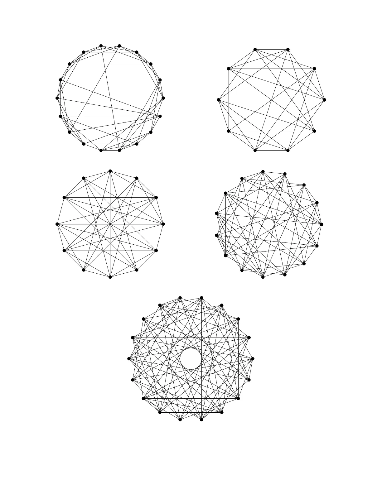
Regular 𝐾 3 -regular graphs Artem Hak ∗ 1, 2 , Sergiy Kozerenk o 2 , Den ys Loh vyno v 3 , and Y urii Y arosh 2, 4 1 National Univ ersity of Kyiv-Moh yla Academ y , 2 Sk ov orody Str., 04070 Kyiv, Ukraine 2 Kyiv Sc ho ol of Economics, 3 Myk oly Shpak a Str., 03113 Kyiv, Ukraine 3 National T ec hnical Universit y of Ukraine “Igor Sik orsky Kyiv P olytechnic Institute”, 37 Beresteiskyi Av e., 03056 Kyiv, Ukraine 4 Kyiv Academic Univ ersity , 36 V ernadsky Blvd., 03142 Kyiv, Ukraine Abstract W e study graphs that are sim ultaneously regular with respect to the ordinary v ertex degree and regular with resp ect to the triangle degree, that is, the n um b er of triangles con taining a giv en v ertex. W e call such graphs regular 𝐾 3 -regular. W e inv estigate the (non-)existence of regular 𝐾 3 -regular graphs with prescrib ed parameters ( 𝑟 2 , 𝑟 3 ), where 𝑟 2 is the vertex degree and 𝑟 3 is the triangle degree. General b ounds relating v ertex and edge triangle degrees are derived, and non-existence results are established for broad ranges of these parameters. Sp ecial atten tion is paid to T ur´ an graphs, for whic h w e establish uniqueness results for certain parameters. The paper concludes with a summary of admissible parameters and sev eral open problems. Keyw ords: vertex degree; triangle degree; regular graph; T ur´ an graph. MSC 2020: 05C07, 05C35, 05C99. 1 In tro duction A graph is called regular if its v ertices ha v e the same degree. A simple application of the pigeonhole principle implies that any graph with at least tw o v ertices has t w o vertices with the same degree. Th us, there are no “irregular” graphs. Nev ertheless, in order to approac h a sensible definition of irregularit y for graphs, Chartrand, Erd˝ os, and Oellermann [ 6 ] prop osed to use the notion of 𝐹 -degree defined in the w ork [ 7 ]. There, for a fixed graph 𝐹 , the 𝐹 -degree of a v ertex 𝑢 from a graph 𝐺 is the n um b er of subgraphs of 𝐺 isomorphic to 𝐹 to whic h 𝑢 b elongs. This w a y , the standard v ertex degree is just the 𝐾 2 -degree. ∗ Corresp onding author: artikgak@ukr.net 1 2 In con trast, for other graphs 𝐹  = 𝐾 2 , there can exist 𝐹 -irregular graphs (i.e., graphs 𝐺 with all v ertices having pairwise distinct 𝐹 -degrees). F or the smallest p ossible 𝐾 3 -irregular graph, see the w ork [ 1 ]. In [ 6 ], the question of whether there exists a regular 𝐾 3 -irregular graph w as p osed. This problem remained op en for sev eral decades until, in 2024, Stev ano vi ´ c et al. [ 10 ] found a 10-regular 𝐾 3 -irregular graph. More recently , the preprin t [ 8 ] gives an example of a 9-regular 𝐾 3 -irregular graph obtained using genetic algorithm tec hniques. It is also shown that there are no suc h graphs for regularities at most 7, with the case of regularity 8 constituting the most in teresting y et op en case (again, see [ 8 ] for the details). F or other asp ects of irregularit y in graphs, w e refer to [ 5 ]. In this paper, w e consider regular 𝐾 3 -regular graphs. Our motiv ation is to further develop the understanding of different regularities a graph can exhibit. The main fo cus is on the (non-)existence of regular 𝐾 3 -regular graphs for the giv en parameters of regularit y . A related framew ork w as in tro duced in [ 9 ], where the authors study v ertex- girth-regular graphs, namely vgr( 𝑛 ; 𝑘 ; 𝑔 ; 𝜆 )-graph is a 𝑘 -regular graph of order 𝑛 and girth 𝑔 in whic h ev ery vertex b elongs to exactly 𝜆 cycles of length 𝑔 . Th us, the graph is regular not only with resp ect to v ertex degrees but also with resp ect to the n um b er of shortest cycles containing eac h vertex. Sev eral non-existence results w ere pro ved for odd 𝑔 ≥ 7 and ev en 𝑔 ≥ 4 (see [ 9 , Theorems 17, 18]). F or the cases 𝑔 = 3 and 𝑔 = 5, the authors form ulate op en questions asking whether the non-existence results from the men tioned theorems hold for these v alues of girth as well. The presen t pap er fo cuses on regular 𝐾 3 -regular graphs, whic h corresp onds precisely to the case 𝑔 = 3. This class of graphs has also already app eared in the literature under a differen t name. In [ 4 ], regular 𝐾 3 -regular graphs with parameters ( 𝑟 2 , 𝑟 3 ) are called ( 𝑟 2 , 𝑟 3 )-constan t graphs. Non-existence result for 𝑟 3 =  𝑟 2 2  − 𝑘 with 𝑘 ∈ N and 3 𝑘 ≤ 𝑟 2 w as pro v en (see [ 4 , Theorem 14]). In [ 3 ], the existence of planar ( 𝑟 2 , 𝑟 3 )-constan t graphs and circulan t ( 𝑟 2 , 𝑟 3 )-constan t graphs is stud- ied. In addition, the authors completely answer the question of the existence of ( 𝑟 2 , 𝑟 3 )-constan t graphs for 𝑟 2 ≤ 6, 𝑟 3 ≤  𝑟 2 2  . Therefore, some basic constrain ts and structural properties of suc h graphs 3 are already kno wn; one of them is the follo wing. Observ ation 1.1. F or every 𝑟 3 ∈ N ∪ { 0 } , ther e exists an inte ger 𝑟 * 2 ∈ N ∪ { 0 } such that (1) for al l 𝑟 2 ≥ 𝑟 * 2 , ther e exists a gr aph with p ar ameters ( 𝑟 2 , 𝑟 3 ) ; (2) for al l 𝑟 2 < 𝑟 * 2 , no gr aph with p ar ameters ( 𝑟 2 , 𝑟 3 ) exists. This observ ation is a simple corollary of a trivial fact that 𝐾 2 and 𝐾 3 are regular 𝐾 3 -regular, and the well-kno wn fact that the degree and 𝐾 3 -degree of a vertex are b oth additiv e under the Cartesian pro duct. As such, w e see that 𝑟 * 2 ≤ 𝑂 ( √ 𝑟 3 ) (consider 𝐾 𝑛 □ 𝐾 3 □ . . . □ 𝐾 3 ). Also, it is w orth men tioning that authors in [ 4 ] impro v ed this b ound to 𝑟 * 2 ≤ 𝑓 − 1 ( 𝑟 3 ), where 𝑓 ( 𝑥 ) = 𝑥 2 2 − 5 𝑥 3 2 (see [ 4 , Theorem 14]). The pap er is organised as follows. In Section 2 , we give all the necessary definitions that will b e used in the pap er. Section 3 is devoted to establishing main tec hnical b ounds for v ertex and edge 𝐾 3 -degrees in regular 𝐾 3 -regular graphs. The imp ortan t results on the non-existence of suc h graphs are pro- vided b y Prop osition 3.5 and Theorem 3.6 . Section 4 con tains results on a w ell-kno wn family of T ur´ an graphs, whic h are pro v ed to b e an imp ortan t class of regular 𝐾 3 -regular graphs. In particular, w e presen t a characterisation of T ur´ an graphs for certain parameters in Theorem 4.1 and in Theorem 4.2 (whic h also demonstrates non-existence). W e conclude the pap er with Sec- tion 5 , presen ting several op en questions and research directions on regular 𝐾 3 -regular graphs. Finally , App endix A contains some examples of regular 𝐾 3 -regular graphs for small regularities, and a table which summarises our results on the existence of these graphs. 2 Main definitions A graph is an ordered pair 𝐺 = ( 𝑉 , 𝐸 ), where 𝑉 = 𝑉 ( 𝐺 ) is the set of its vertic es and 𝐸 = 𝐸 ( 𝐺 ) ⊂  𝑉 2  is the set of its e dges . All the graphs considered in this pap er are undirected, simple and finite. Also, for a pair of vertices 𝑢, 𝑣 ∈ 𝑉 ( 𝐺 ), the edge { 𝑢, 𝑣 } will b e denoted as 𝑢𝑣 . By 𝐺 , w e denote the 4 c omplement of a graph 𝐺 . The complete graph with 𝑛 v ertices is denoted b y 𝐾 𝑛 . The op en neighb ourho o d of a v ertex 𝑣 in a graph 𝐺 is the set of all its adjacen t v ertices: 𝑁 ( 𝑣 ) = { 𝑢 ∈ 𝑉 ( 𝐺 ) : 𝑢𝑣 ∈ 𝐸 ( 𝐺 ) } . The close d neigh- b ourho o d of 𝑣 is the set 𝑁 [ 𝑣 ] = 𝑁 ( 𝑣 ) ∪ { 𝑣 } . The de gr e e of 𝑣 in 𝐺 is the n um b er deg ( 𝑣 ) = | 𝑁 ( 𝑣 ) | . A v ertex 𝑣 ∈ 𝑉 ( 𝐺 ) is an isolate d vertex provided deg( 𝑣 ) = 0. The graph 𝐺 is said to b e r e gular if all its vertices ha v e the same degree, whic h is called the r e gularity of 𝐺 . Tw o graphs 𝐺 and 𝐻 are called isomorphic if there is an isomorphism b et w een them, that is, a bijection 𝑓 : 𝑉 ( 𝐺 ) → 𝑉 ( 𝐻 ) suc h that 𝑢𝑣 ∈ 𝐸 ( 𝐺 ) if and only if 𝑓 ( 𝑢 ) 𝑓 ( 𝑣 ) ∈ 𝐸 ( 𝐺 ). Giv en v ertices 𝑣 1 , . . . , 𝑣 𝑘 ∈ 𝑉 ( 𝐺 ), b y 𝐺 [ 𝑣 1 , . . . , 𝑣 𝑘 ] w e denote the sub- graph induced by the union of their closed neighbourho o ds  𝑘 𝑖 =1 𝑁 [ 𝑣 𝑖 ], and b y 𝐺 ( 𝑣 1 , . . . , 𝑣 𝑘 ) we denote the subgraph induced by the union of their op en neigh b ourho ods  𝑘 𝑖 =1 𝑁 ( 𝑣 𝑖 ). The Cartesian pr o duct of tw o graphs 𝐺 1 and 𝐺 2 is the graph 𝐺 1 □ 𝐺 2 with 𝑉 ( 𝐺 1 □ 𝐺 2 ) = 𝑉 ( 𝐺 1 ) × 𝑉 ( 𝐺 2 ), and tw o v ertices ( 𝑢, 𝑣 ) and ( 𝑢 ′ , 𝑣 ′ ) b eing adjacen t if and only if either 𝑢 = 𝑢 ′ and 𝑣 𝑣 ′ ∈ 𝐸 ( 𝐺 2 ), or 𝑣 = 𝑣 ′ and 𝑢𝑢 ′ ∈ 𝐸 ( 𝐺 1 ). Definition 2.1 ([ 6 , 7 ]) . F or a given graph 𝐹 , the 𝐹 -de gr e e of a v ertex 𝑣 in 𝐺 is the n um b er 𝐹 deg( 𝑣 ) of subgraphs of 𝐺 , isomorphic to 𝐹 , to which 𝑣 b elongs. Note that the ordinary degree of a vertex is exactly its 𝐾 2 -degree. Also, it is readily seen that 𝐾 3 deg( 𝑣 ) = |  𝑁 ( 𝑣 ) 2  ∩ 𝐸 ( 𝐺 ) | . Definition 2.2. F or a giv en graph 𝐹 , the 𝐹 -de gr e e of an edge 𝑒 ∈ 𝐸 ( 𝐺 ) is the num b er 𝐹 deg ( 𝑒 ) of subgraphs of 𝐺 , isomorphic to 𝐹 , to which 𝑒 b elongs. Note that 𝐾 3 deg( 𝑢𝑣 ) = | 𝑁 ( 𝑢 ) ∩ 𝑁 ( 𝑣 ) | for any edge 𝑢𝑣 ∈ 𝐸 ( 𝐺 ). Definition 2.3. A graph is called 𝐾 3 -regular if all its vertices ha v e the same 𝐾 3 -degree. Throughout the pap er, w e fo cus on graphs that are b oth regular and 𝐾 3 -regular. If 𝐺 is such a graph, we denote by 𝑟 2 the common 𝐾 2 -degree 5 (i.e., the ordinary degree) of all its v ertices, and by 𝑟 3 the common 𝐾 3 -degree of all its v ertices. W e sa y that 𝐺 has p ar ameters ( 𝑟 2 , 𝑟 3 ) if 𝐺 is regular with degree 𝑟 2 and 𝐾 3 -regular with 𝐾 3 -degree 𝑟 3 . Definition 2.4. T ur´ an graphs are complete multipartite graphs built b y par- titioning a set of 𝑛 vertices in to 𝑟 subsets as equally as p ossible and connecting ev ery pair of v ertices that lie in differen t parts. In this pap er, w e restrict ourselv es to the case where 𝑟 | 𝑛 , so that all parts ha v e equal size (also known as complete m ultipartite graphs). These graphs were in tro duced in T ur´ an’s classical 1941 pap er [ 12 ]. W e shall denote these graphs b y T uran( 𝑛, 𝑟 ). Assume that 𝑟 | 𝑛 , then T ur´ an graphs are regular and, moreo v er, 𝐾 3 - regular. F or 𝑟 ≥ 3, we can explicitly calculate the regularity parameters 𝑟 2 = 𝑛 𝑟 ( 𝑟 − 1) , 𝑟 3 =  𝑟 − 1 2  ·  𝑛 𝑟  2 . 3 Establishing b ounds In this section, w e establish fundamental b ounds on the parameters of 𝐾 3 - regular graphs. W e deriv e several direct estimates and dev elop key technical lemmas relating edge 𝐾 3 -degrees to v ertex degrees. These results form the main to ols for the non-existence theorems prov ed in the subsequen t sections. The follo wing lemma giv es a trivial but useful upper b ound on the param- eter 𝑟 3 in terms of 𝑟 2 . Lemma 3.1. F or every gr aph with p ar ameters ( 𝑟 2 , 𝑟 3 ) , the fol lowing upp er b ound holds: 𝑟 3 ≤  𝑟 2 2  . 3.1 Edge degree statemen ts The following Lemmas 3.2 , 3.3 and 3.4 are considered instrumen tal since what they pro vide is sev eral relations b et w een the edge 𝐾 3 -degree and v ertex degrees without giving an y tangible constrain ts on the parameters righ t a w a y . 6 Nev ertheless, they will pla y a crucial role in subsequen t existence and non- existence argumen ts. The following lemma follo ws directly from the handshaking lemma, and it will b e used several times throughout the article. Lemma 3.2. F or any gr aph 𝐺 and any vertex 𝑣 , we have 𝐾 3 deg( 𝑣 ) = 1 2  𝑢 ∈ 𝑁 ( 𝑣 ) 𝐾 3 deg( 𝑢𝑣 ) . Pr o of. Consider the induced subgraph 𝐻 = 𝐺 ( 𝑣 ). Eac h triangle of 𝐺 con tain- ing 𝑣 corresp onds to an edge of 𝐻 , therefore 𝐾 3 deg 𝐺 ( 𝑣 ) = | 𝐸 ( 𝐻 ) | . Moreo v er, for ev ery 𝑢 ∈ 𝑉 ( 𝐻 ), w e ha v e 𝐾 3 deg 𝐺 ( 𝑢𝑣 ) = deg 𝐻 ( 𝑢 ) . Applying the handshaking lemma to 𝐻 yields 1 2  𝑢 ∈ 𝑉 ( 𝐻 ) 𝐾 3 deg 𝐺 ( 𝑢𝑣 ) = 1 2  𝑢 ∈ 𝑉 ( 𝐻 ) deg 𝐻 ( 𝑢 ) = | 𝐸 ( 𝐻 ) | = 𝐾 3 deg 𝐺 ( 𝑣 ) , whic h completes the pro of. The next lemma giv es an upp er b ound for the 𝐾 3 -degrees of edges in regular 𝐾 3 -regular graphs. Lemma 3.3. L et 𝐺 b e a gr aph with p ar ameters ( 𝑟 2 , 𝑟 3 ) . Then, for any e dge 𝑒 ∈ 𝐸 ( 𝐺 ) , the fol lowing upp er b ound holds: 𝐾 3 deg( 𝑒 ) ≤ min { 𝑟 3 , 𝑟 2 − 1 } . Pr o of. Fix an edge 𝑒 = 𝑢𝑤 ∈ 𝐸 ( 𝐺 ). By definition, 𝐾 3 deg( 𝑒 ) = | 𝑁 ( 𝑢 ) ∩ 𝑁 ( 𝑤 ) | . Since, 𝑁 ( 𝑢 ) ∩ 𝑁 ( 𝑤 ) ⊆ 𝑁 ( 𝑢 ) ∩ ( 𝑁 ( 𝑤 ) ∖ { 𝑢 } ), we obtain 𝐾 3 deg( 𝑒 ) ≤ | 𝑁 ( 𝑤 ) ∖ { 𝑢 }| ≤ 𝑟 2 − 1 . On the other hand, eac h v ertex 𝑣 ∈ 𝑁 ( 𝑢 ) ∩ 𝑁 ( 𝑤 ) determines a triangle { 𝑢, 𝑤 , 𝑣 } con taining 𝑢 . Hence, 𝐾 3 deg( 𝑒 ) ≤ 𝐾 3 deg( 𝑢 ) = 𝑟 3 , and the claim follo ws. 7 The follo wing lemma complements the previous result by relating edge 𝐾 3 -degrees to the regularit y parameters. Lemma 3.4. L et 𝐺 b e a gr aph with p ar ameters ( 𝑟 2 , 𝑟 3 ) and let 𝑒 ∈ 𝐸 ( 𝐺 ) b e an e dge with 𝐾 3 deg( 𝑒 ) = 𝑘 . Then the fol lowing ine quality holds: 2 𝑟 3 ≤ ( 𝑟 2 − 𝑘 − 1)( 𝑟 2 − 2) + 𝑘 ( 𝑘 + 1) . Pr o of. Let 𝐺 b e a graph with parameters ( 𝑟 2 , 𝑟 3 ) and let 𝑢𝑣 ∈ 𝐸 ( 𝐺 ). Set 𝐾 3 deg( 𝑢𝑣 ) = | 𝑁 ( 𝑢 ) ∩ 𝑁 ( 𝑣 ) | = 𝑘 . F or a v ertex 𝑥 ∈ 𝑉 ( 𝐺 ), denote b y △ ( 𝑥 ) the set of all triangles containing 𝑥 . Our first step is to estimate the size of the set △ ( 𝑢 ) ∪ △ ( 𝑣 ). Define 𝐶 = 𝑁 ( 𝑢 ) ∩ 𝑁 ( 𝑣 ) = { 𝑤 1 , . . . , 𝑤 𝑘 } , 𝐼 1 = 𝑁 ( 𝑢 ) ∖ 𝑁 [ 𝑣 ] , 𝐼 2 = 𝑁 ( 𝑣 ) ∖ 𝑁 [ 𝑢 ] , put 𝑖 = | 𝐼 1 | = | 𝐼 2 | = 𝑟 2 − 𝑘 − 1. Let 𝐺 ′ b e a subgraph induced b y 𝐶 , and for eac h 𝑤 𝑗 ∈ 𝐶 set 𝑑 𝑗 = deg 𝐺 ′ ( 𝑤 𝑗 ). Note that 0 ≤ 𝑑 𝑗 ≤ 𝑘 − 1. No w, ha ving tak en care of the prerequisites, we shall pro ceed b y calculat- ing |△ ( 𝑢 ) ∪ △ ( 𝑣 ) | . On the one hand, |△ ( 𝑢 ) ∪ △ ( 𝑣 ) | = |△ ( 𝑢 ) | + |△ ( 𝑣 ) | − |△ ( 𝑢 ) ∩ △ ( 𝑣 ) | = 𝑟 3 + 𝑟 3 − | 𝐶 | = 2 𝑟 3 − 𝑘 . On the other hand, let △ 𝐴𝐵 𝐶 denote the set of triangles ha ving one v ertex in each of 𝐴 , 𝐵 , and 𝐶 (where single v ertices are iden tified with singleton sets). W e decomp ose the set △ ( 𝑢 ) ∪ △ ( 𝑣 ) in to the follo wing disjoin t subsets: △ ( 𝑢 ) ∪ △ ( 𝑣 ) = ( △ 𝐼 1 𝐼 1 𝑢 ⊔ △ 𝐼 2 𝐼 2 𝑣 ) ⊔ △ 𝐶 𝑢𝑣 ⊔ ( △ 𝐶 𝐶 𝑢 ∪ △ 𝐶 𝐶 𝑣 ) ⊔ ( △ 𝐶 𝐼 1 𝑢 ∪ △ 𝐶 𝐼 2 𝑣 ) . W e estimate the cardinalities of these sets separately: • Clearly , |△ 𝐼 1 𝐼 1 𝑢 ⊔ △ 𝐼 2 𝐼 2 𝑣 | ≤ 2  𝑖 2  . • The num b er of triangles con taining 𝑢 , 𝑣 and one v ertex of 𝐶 is exactly |△ 𝐶 𝑢𝑣 | = | 𝐶 | = 𝑘 . 8 • Each edge of 𝐺 ′ con tributes to exactly t w o triangles, one con taining 𝑢 and one con taining 𝑣 , therefore |△ 𝐶 𝐶 𝑢 ∪ △ 𝐶 𝐶 𝑣 | = 2 | 𝐸 ( 𝐺 ′ ) | = 𝑘  𝑗 =1 𝑑 𝑗 . • Finally , consider the term |△ 𝐶 𝐼 1 𝑢 ∪ △ 𝐶 𝐼 2 𝑣 | . Each v ertex 𝑤 𝑗 is adjacent to 𝑑 𝑗 v ertices from 𝐶 and to 𝑢 and 𝑣 . Hence, 𝑤 𝑗 cannot con tribute more than 𝑟 2 − 𝑑 𝑗 − 2 triangles of the aforementioned t yp e. Th us, |△ 𝐶 𝐼 1 𝑢 ∪ △ 𝐶 𝐼 2 𝑣 | ≤ 𝑘  𝑗 =1 ( 𝑟 2 − 𝑑 𝑗 − 2) . Summing it all up, w e obtain 2 𝑟 3 − 𝑘 = |△ ( 𝑢 ) ∪ △ ( 𝑣 ) | ≤ 2  𝑖 2  + 𝑘 + 𝑘  𝑗 =1 𝑑 𝑗 + 𝑘  𝑗 =1 ( 𝑟 2 − 𝑑 𝑗 − 2) = 2  𝑖 2  + ( 𝑟 2 − 1) 𝑘 . Substituting 𝑖 = 𝑟 2 − 𝑘 − 1 and rearranging yields the stated inequality . 3.2 Non-trivial b ounds on the parameters The following t w o statements pro vide some non-trivial restrictions on the pa- rameters ( 𝑟 2 , 𝑟 3 ) for whic h there exists a regular 𝐾 3 -regular graph. It is w orth noting that [ 3 , Prop osition 14] states the non-existence of graphs with param- eters (5 , 7) , (5 , 8) and (6 , 11) b y lo oking sp ecifically at their inner structure. Our next results v astly generalise this fact. The next prop osition is pro v ed b y virtue of com bining the three lemmas from the previous subsection. Prop osition 3.5. Ther e ar e no gr aphs with p ar ameters ( 𝑟 2 , 𝑟 3 ) such that 𝑟 3 =  𝑟 2 − 1 2  + 𝑐 for 𝑟 2 > 4 and 0 < 𝑐 < 𝑟 2 − 2 2 . 9 Pr o of. Supp ose that 𝐺 is a regular 𝐾 3 -regular graph with 𝑟 3 =  𝑟 2 − 1 2  + 𝑐 . Fix an arbitrary edge 𝑒 ∈ 𝐸 ( 𝐺 ) and put 𝑘 = 𝐾 3 deg( 𝑒 ). By virtue of Lemma 3.3 , w e ha v e 𝑘 ≤ 𝑟 2 − 1. Moreov er, Lemma 3.4 yields 2  𝑟 2 − 1 2  + 𝑐  = 2 𝑟 3 ≤ ( 𝑟 2 − 1 − 𝑘 )( 𝑟 2 − 2) + 𝑘 ( 𝑘 + 1) . Solving the quadratic inequalit y in 𝑘 , w e obtain 𝑘 ≥ 𝑟 2 − 3 2 +  2 𝑐 +  𝑟 2 − 3 2  2 > 𝑟 2 − 3 or 𝑘 ≤ 𝑟 2 − 3 2 −  2 𝑐 +  𝑟 2 − 3 2  2 < 0 . Since 𝑘 ≥ 0, the latter case is imp ossible and, therefore, 𝑘 ∈ { 𝑟 2 − 2 , 𝑟 2 − 1 } . Fix an arbitrary v ertex 𝑣 ∈ 𝑉 ( 𝐺 ). Among the 𝑟 2 edges incident to 𝑣 , let 𝑎 and 𝑏 denote the n um b ers of edges 𝑣 𝑢 of 𝐾 3 -degree 𝑟 2 − 2 and 𝑟 2 − 1, resp ectiv ely . Then 𝑎 + 𝑏 = 𝑟 2 . By Lemma 3.2 , w e obtain 2 𝐾 3 deg( 𝑣 ) =  𝑢 ∈ 𝑁 ( 𝑣 ) 𝐾 3 deg( 𝑢𝑣 ) , 2 𝑟 3 = 2  𝑟 2 − 1 2  + 𝑐  = ( 𝑟 2 − 2) 𝑎 + ( 𝑟 2 − 1) 𝑏, 𝑎 + 𝑏 = 𝑟 2 , 𝑎, 𝑏 ≥ 0 . Using 𝑐 < 𝑟 2 − 2 2 , w e ha v e ( 𝑟 2 − 2) 𝑎 + ( 𝑟 2 − 1) 𝑏 = 2  𝑟 2 − 1 2  + 𝑐  < 𝑟 2 2 − 2 𝑟 2 , 𝑟 2 ( 𝑎 + 𝑏 ) − ( 𝑎 + 𝑏 ) − 𝑎 < 𝑟 2 2 − 2 𝑟 2 , 𝑟 2 < 𝑎. This leads to a con tradiction. Hence, there are no suc h graphs. The follo wing theorem establishes the non-existence result for a range of regularit y parameters. In particular, it excludes such pairs of parameters 10 ( 𝑟 2 , 𝑟 3 ) as (4 , 5) and (5 , 9), whic h app ear in T able 1 in Appendix A (see Corol- laries 3.7 and 3.8 ). Our theorem improv es up on [ 11 , Theorem 2]; in particular, w e exclude one more parameter for every o dd 𝑟 2 b y using a differen t pro of tec hnique. Moreo v er, this result affirmativ ely answers the question p osed in [ 9 ] regarding the existence of vgr( 𝑛, 𝑟 2 , 3 , 𝑟 3 )-graphs (see Theorems 17, 18 and the discussion afterw ards therein). Theorem 3.6. Ther e exists no gr aph with p ar ameters ( 𝑟 2 , 𝑟 3 ) such that 𝑟 3 =  𝑟 2 2  − 𝑐 , pr ovide d 𝑟 2 ≥ 3 and 1 ≤ 𝑐 ≤ 𝑟 2 − 1 2 . Pr o of. Supp ose, for the sake of con tradiction, that such a graph 𝐺 exists. Let 𝑣 ∈ 𝑉 ( 𝐺 ) b e an arbitrary v ertex and let 𝐺 [ 𝑣 ] b e the subgraph induced by the closed neigh b ourhoo d of 𝑣 . Note that the 𝐾 3 -degree of 𝑣 equals the num b er of edges in its op en neighbourho o d, namely , | 𝐸 ( 𝐺 ( 𝑣 )) | = 𝐾 3 deg( 𝑣 ) =  𝑟 2 2  − 𝑐. Therefore, the minimum degree in 𝐺 [ 𝑣 ] is at least 𝑟 2 − 𝑐 . Fix a v ertex 𝑢 ∈ 𝑁 [ 𝑣 ] of suc h degree in 𝐺 [ 𝑣 ]. Hence, deg 𝐺 [ 𝑣 ] ( 𝑢 ) = 𝑟 2 − 𝑑 , where 1 ≤ 𝑑 ≤ 𝑐 . Since deg 𝐺 [ 𝑣 ] ( 𝑢 ) < 𝑟 2 , there exists a v ertex 𝑤 ∈ 𝑉 ( 𝐺 ) ∖ 𝑁 [ 𝑣 ] suc h that 𝑤 𝑢 ∈ 𝐸 ( 𝐺 ). F or 𝑘 ∈ { 𝑟 2 − 𝑑, . . . , 𝑟 2 − 1 } , define 𝐵 𝑘 = { 𝑣 ′ ∈ 𝑁 ( 𝑣 ) : deg 𝐺 [ 𝑣 ] ( 𝑣 ′ ) = 𝑘 } , 𝐵 ′ 𝑘 = { 𝑣 ′ ∈ 𝐵 𝑘 : 𝑣 ′ 𝑤 ∈ 𝐸 } . Note that 𝑢 ∈ 𝐵 ′ 𝑟 2 − 𝑑 b y construction (see Figure 1a ). Also, denote their unions as 𝐵 = 𝑟 2 − 1  𝑘 = 𝑟 2 − 𝑑 𝐵 𝑘 and 𝐵 ′ = 𝑟 2 − 1  𝑘 = 𝑟 2 − 𝑑 𝐵 ′ 𝑘 . The handshaking lemma applied to the complemen t of 𝐺 [ 𝑣 ] yields 𝑟 2 − 1  𝑗 = 𝑟 2 − 𝑑 ( 𝑟 2 − 𝑗 ) | 𝐵 𝑗 | = 2 𝑐. (1) In order to reac h the contradiction, w e will find an upp er b ound for the 𝐾 3 -degree of 𝑤 . F or 𝑏 𝑘 = | 𝐵 ′ 𝑘 | , w e ha v e the follo wing constrain ts: 𝑏 𝑘 ≥ 0 , 𝑏 𝑟 2 − 𝑑 ≥ 1 , 𝑏 𝑟 2 − 1 + 2 𝑏 𝑟 2 − 2 + . . . + 𝑑𝑏 𝑟 2 − 𝑑 ≤ 2 𝑐. 11 Denote 𝐼 = 𝑁 ( 𝑤 ) ∖ 𝑁 [ 𝑣 ], and observ e the follo wing: | 𝐼 | + 𝑏 𝑟 2 − 1 + . . . + 𝑏 𝑟 2 − 𝑑 = deg 𝐺 ( 𝑤 ) = 𝑟 2 . (2) 𝑣 𝑤 𝑁 ( 𝑣 ) 𝐵 𝑟 2 − 𝑑 . . . 𝐵 𝑟 2 − 1 rest of 𝑁 ( 𝑣 ) 𝑢 (a) Schematic illustration of the sets 𝐵 𝑖 . 𝑁 ( 𝑣 ) 𝐼 𝑣 𝑢 𝑤 Δ 𝐼 𝑤 𝐼 Δ 𝐵 ′ 𝑤 𝐼 Δ 𝐵 ′ 𝑤 𝐵 ′ (b) The three t ypes of triangles. Figure 1. Constructions in Theorem 3.6 . No w w e split the triangles con taining 𝑤 in to three t yp es (see Figure 1b ) and coun t the size of eac h t yp e. T yp e 1: △ 𝐼 𝑤 𝐼 . These are triangles with t w o vertices in 𝐼 and one v ertex 𝑤 . Clearly , |△ 𝐼 𝑤 𝐼 | ≤  | 𝐼 | 2  . (3) T yp e 2: △ 𝐵 ′ 𝑤 𝐼 . These are triangles with one v ertex in 𝐼 , one in 𝐵 ′ and the v ertex 𝑤 . If 𝑥 ∈ 𝐵 ′ 𝑟 2 − 𝑖 , then 𝑥 has exactly 𝑖 non-neigh b ours in 𝐺 [ 𝑣 ]. Also, 𝑥 is adjacent to 𝑤 . Hence, 𝑥 can b e adjacen t to at most 𝑖 − 1 v ertices of 𝐼 . Therefore, |△ 𝐵 ′ 𝑤 𝐼 | ≤ 𝑑  𝑖 =1 ( 𝑖 − 1) 𝑏 𝑟 2 − 𝑖 = 𝑏 𝑟 2 − 2 + 2 𝑏 𝑟 2 − 3 + . . . + ( 𝑑 − 1) 𝑏 𝑟 2 − 𝑑 . (4) T yp e 3: △ 𝐵 ′ 𝑤 𝐵 ′ . These are triangles with t w o vertices in 𝐵 ′ and the v ertex 𝑤 . W e hav e |△ 𝐵 ′ 𝑤 𝐵 ′ | =      𝐵 ′ 2  ∩ 𝐸 ( 𝐺 )     =      𝐵 ′ 2      −      𝐵 ′ 2  ∖ 𝐸 ( 𝐺 )     . 12 W e shall mak e use of the follo wing set equalit y:  𝑌 2  =  𝑋 2  ⊔  𝑌 ∖ 𝑋 2  ⊔ ( 𝑋 ^ × 𝑌 ) , where 𝑋 ⊆ 𝑌 and 𝑋 ^ × 𝑌 = {{ 𝑥, 𝑦 } : 𝑥 ∈ 𝑋 , 𝑦 ∈ 𝑌 ∖ 𝑋 } . Apply this set equalit y to 𝐵 ′ ⊆ 𝐵 and express  𝐵 ′ 2  from it  𝐵 ′ 2  =  𝐵 2  ∖  𝐵 ∖ 𝐵 ′ 2  ⊔ ( 𝐵 ′ ^ × 𝐵 )  . As a result, b y virtue of straightforw ard set-theoretic manipulations, we ha v e that  𝐵 ′ 2  ∖ 𝐸 ( 𝐺 ) =  𝐵 2  ∖ 𝐸 ( 𝐺 )  ∖  𝐵 ∖ 𝐵 ′ 2  ⊔ ( 𝐵 ′ ^ × 𝐵 )  ∖ 𝐸 ( 𝐺 )  . Th us, using ( 2 ) w e obtain |△ 𝐵 ′ 𝑤 𝐵 ′ | =  𝑏 𝑟 2 − 1 + . . . + 𝑏 𝑟 2 − 𝑑 2  − −      𝐵 2  ∖ 𝐸 ( 𝐺 )  ∖  𝐵 ∖ 𝐵 ′ 2  ⊔ ( 𝐵 ′ ^ × 𝐵 )  ∖ 𝐸 ( 𝐺 )      =  𝑟 2 − | 𝐼 | 2  −      𝐵 2  ∖ 𝐸 ( 𝐺 )     +      𝐵 ∖ 𝐵 ′ 2  ⊔ ( 𝐵 ′ ^ × 𝐵 )  ∖ 𝐸 ( 𝐺 )     =  𝑟 2 − | 𝐼 | 2  − 𝑐 +      𝐵 ∖ 𝐵 ′ 2  ⊔ ( 𝐵 ′ ^ × 𝐵 )  ∖ 𝐸 ( 𝐺 )     . (5) W e no w estimate the last term. First of all, it is readily seen that  𝐵 ∖ 𝐵 ′ 2  ⊔ ( 𝐵 ′ ^ × 𝐵 ) =  𝑥 ∈ 𝐵 ∖ 𝐵 ′ {{ 𝑥, 𝑦 } : 𝑦 ∈ 𝐵 ∖ { 𝑥 }} . Recalling definitions of 𝐵 and 𝐵 ′ , we obtain that 𝐵 ∖ 𝐵 ′ =  𝑟 2 − 1 𝑖 = 𝑟 2 − 𝑑 ( 𝐵 𝑖 ∖ 𝐵 ′ 𝑖 ). Th us,  𝐵 ∖ 𝐵 ′ 2  ⊔ ( 𝐵 ′ ^ × 𝐵 ) = 𝑟 2 − 1  𝑖 = 𝑟 2 − 𝑑  𝑥 ∈ 𝐵 𝑖 ∖ 𝐵 ′ 𝑖 {{ 𝑥, 𝑦 } : 𝑦 ∈ 𝐵 ∖ { 𝑥 }} . Hence, w e obtain that      𝐵 ∖ 𝐵 ′ 2  ⊔ ( 𝐵 ′ ^ × 𝐵 )  ∖ 𝐸 ( 𝐺 )     ≤ 𝑟 2 − 1  𝑖 = 𝑟 2 − 𝑑  𝑥 ∈ 𝐵 𝑖 ∖ 𝐵 ′ 𝑖 |{{ 𝑥, 𝑦 } : 𝑦 ∈ 𝐵 ∖ { 𝑥 }}∖ 𝐸 ( 𝐺 ) | . 13 Also, for 𝑥 ∈ 𝐵 𝑖 ∖ 𝐵 ′ 𝑖 , w e ha v e deg 𝑁 [ 𝑣 ] ( 𝑥 ) = 𝑖 . Hence, |{{ 𝑥, 𝑦 } : 𝑦 ∈ 𝐵 ∖ { 𝑥 }} ∖ 𝐸 ( 𝐺 ) | = |{ 𝑦 ∈ 𝐵 ∖ { 𝑥 } : 𝑥𝑦 / ∈ 𝐸 ( 𝐺 ) }| ≤ |{ 𝑦 ∈ 𝑁 [ 𝑣 ] ∖ { 𝑥 } : 𝑥𝑦 / ∈ 𝐸 ( 𝐺 ) }| = deg 𝑁 [ 𝑣 ] ( 𝑥 ) = 𝑟 2 − deg 𝑁 [ 𝑣 ] ( 𝑥 ) = 𝑟 2 − 𝑖. Th us, w e finish the calculations using ( 1 ) and ( 4 )      𝐵 ∖ 𝐵 ′ 2  ⊔ ( 𝐵 ′ ^ × 𝐵 )  ∖ 𝐸 ( 𝐺 )     ≤ 𝑟 2 − 1  𝑖 = 𝑟 2 − 𝑑 ( 𝑟 2 − 𝑖 ) | 𝐵 𝑖 ∖ 𝐵 ′ 𝑖 | = 𝑟 2 − 1  𝑖 = 𝑟 2 − 𝑑 ( 𝑟 2 − 𝑖 ) | 𝐵 𝑖 | − 𝑟 2 − 1  𝑖 = 𝑟 2 − 𝑑 ( 𝑟 2 − 𝑖 ) | 𝐵 ′ 𝑖 | = 2 𝑐 − ( 𝑏 𝑟 2 − 1 + 2 𝑏 𝑟 2 − 2 + . . . + 𝑑𝑏 𝑟 2 − 𝑑 ) . (6) Therefore, substituting ( 6 ) in to ( 5 ), w e get |△ 𝐵 ′ 𝑤 𝐵 ′ | ≤  𝑟 2 − | 𝐼 | 2  + 𝑐 − ( 𝑏 𝑟 2 − 1 + 2 𝑏 𝑟 2 − 2 + . . . + 𝑑𝑏 𝑟 2 − 𝑑 ) . (7) Th us, w e ha v e estimated all three triangle t yp es. Summing up inequali- ties ( 3 ), ( 4 ) and ( 7 ), w e get an upp er b ound 𝐾 3 deg( 𝑤 ) = |△ 𝐼 𝑤 𝐼 | + |△ 𝐵 ′ 𝑤 𝐼 | + |△ 𝐵 ′ 𝑤 𝐵 ′ | ≤  | 𝐼 | 2  + 𝑏 𝑟 2 − 2 + 2 𝑏 𝑟 2 − 3 + . . . + ( 𝑑 − 1) 𝑏 𝑟 2 − 𝑑 +  𝑟 2 − | 𝐼 | 2  + 𝑐 − ( 𝑏 𝑟 2 − 1 + 2 𝑏 𝑟 2 − 2 + . . . + 𝑑𝑏 𝑟 2 − 𝑑 ) . Simplifying, w e get 𝐾 3 deg( 𝑤 ) ≤  | 𝐼 | 2  +  𝑟 2 − | 𝐼 | 2  + 𝑐 − ( 𝑏 𝑟 2 − 1 + 𝑏 𝑟 2 − 2 + . . . + 𝑏 𝑟 2 − 𝑑    this equals 𝑟 2 −| 𝐼 | b y ( 2 ) ) =  | 𝐼 | 2  +  𝑟 2 − | 𝐼 | 2  + 𝑐 − 𝑟 2 + | 𝐼 | . Define the function 𝐹 ( 𝑥 ) =  𝑥 2  +  𝑟 2 − 𝑥 2  + 𝑐 − 𝑟 2 + 𝑥 = 𝑥 2 − 𝑥 ( 𝑟 2 − 1) + 𝑐 + 𝑟 2 2 − 3 𝑟 2 2 . 14 No w, let us deriv e stricter constraints on 𝑥 := | 𝐼 | . Starting with an upp er b ound 𝑥 ≤ | 𝐼 | + 𝑏 𝑟 2 − 1 + . . . + 𝑏 𝑟 2 − 𝑑 − 1 = 𝑟 2 − 1 . And in a similar manner, w e deriv e a lo w er b ound 𝑥 ≥ | 𝐼 | − ( 𝑏 𝑟 2 − 2 + 2 𝑏 𝑟 2 − 3 + . . . + ( 𝑑 − 1) 𝑏 𝑟 2 − 𝑑 ) = 𝑟 2 − ( 𝑏 𝑟 2 − 1 + 2 𝑏 𝑟 2 − 2 + . . . + 𝑑𝑏 𝑟 2 − 𝑑 ) ≥ 𝑟 2 − 2 𝑐. Hence, w e see that max 𝐾 3 deg( 𝑤 ) ≤ max  𝐹 ( 𝑥 ) : 𝑟 2 − 2 𝑐 ≤ 𝑥 ≤ 𝑟 2 − 1  . W e no w determine the maxim um of 𝐹 on this in terv al. First of all, 𝐹 is a quadratic function with a p ositiv e leading co efficien t. Therefore, the maxim um is attained at one of the endp oin ts, namely either 𝑥 = 𝑟 2 − 1 or 𝑥 = 𝑟 2 − 2 𝑐 𝐹 ( 𝑟 2 − 1) − 𝐹 ( 𝑟 2 − 2 𝑐 ) = ( 𝑟 2 − 2 𝑐 )(2 𝑐 − 1) ≥ 1 . Th us, the maximum v alue is 𝐹 ( 𝑟 2 − 1) =  𝑟 2 − 1 2  + 𝑐 − 1. F or 1 ≤ 𝑐 ≤ 𝑟 2 − 1 2 , w e ha v e 𝐹 ( 𝑟 2 − 1) <  𝑟 2 2  − 𝑐, whic h yields the con tradiction 𝐾 3 deg( 𝑤 ) ≤ 𝐹 ( 𝑟 2 − 1) <  𝑟 2 2  − 𝑐 = 𝑟 3 . W e can summarise the findings of this subsection in the follo wing tw o corollaries. Corollary 3.7. L et 𝑟 2 ≥ 4 b e an even inte ger. Then ther e ar e no gr aphs with p ar ameters ( 𝑟 2 , 𝑟 3 ) , wher e 4  0 . 5 𝑟 2 2  < 𝑟 3 <  𝑟 2 2  or  𝑟 2 − 1 2  < 𝑟 3 < 4  0 . 5 𝑟 2 2  . Mor e over, one example of a gr aph that c orr esp onds to 𝑟 3 =  𝑟 2 2  is 𝐾 𝑟 2 +1 , an example that c orr esp onds to 𝑟 3 = 4  0 . 5 𝑟 2 2  is T uran( 𝑟 2 + 2 , 0 . 5 𝑟 2 + 1) , and an example that c orr esp onds to 𝑟 3 =  𝑟 2 − 1 2  is 𝐾 𝑟 2 □ 𝐾 2 . 15 Pr o of. First of all, it is easy to verify that 𝐾 𝑟 2 +1 , T uran( 𝑟 2 + 2 , 0 . 5 𝑟 2 + 1) and 𝐾 𝑟 2 □ 𝐾 2 are the aforemen tioned examples. No w, assume the pair ( 𝑟 2 , 𝑟 3 ) satisfies the first inequality . In this case, w e use Theorem 3.6 . Indeed, we can represent 𝑟 3 that satisfies the inequalit y as  𝑟 2 2  − 𝑐 , where 𝑐 ∈ { 1 , . . . ,  𝑟 2 2  − 4  0 . 5 𝑟 2 2  − 1 } . Let us simplify the v alue  𝑟 2 2  − 4  0 . 5 𝑟 2 2  − 1 = 𝑟 2 − 2 2 . So, we see that 𝑐 ≥ 1 and 𝑟 2 ≥ 2 𝑐 + 2 > 2 𝑐 + 1. Th us, the aforemen tioned theorem applies. No w, let ( 𝑟 2 , 𝑟 3 ) satisfy the second inequalit y . Observ e that in this case 𝑟 2 > 4. Hence, using Prop osition 3.5 , w e see that there are no graphs with 𝑟 3 =  𝑟 2 − 1 2  + 𝑐 , 𝑐 ∈ { 1 , . . . , 0 . 5 𝑟 2 − 2 } . But 4  0 . 5 𝑟 2 2  − 1 −  𝑟 2 − 1 2  = 0 . 5 𝑟 2 − 2, so w e get that there are no graphs with  𝑟 2 − 1 2  < 𝑟 3 < 4  0 . 5 𝑟 2 2  . Corollary 3.8. L et 𝑟 2 ≥ 3 b e an o dd inte ger. Then ther e ar e no gr aphs with p ar ameters ( 𝑟 2 , 𝑟 3 ) , wher e  𝑟 2 − 1 2  < 𝑟 3 <  𝑟 2 2  . Mor e over, one example of a gr aph that c orr esp onds to 𝑟 3 =  𝑟 2 2  is 𝐾 𝑟 2 +1 and an example that c orr esp onds to 𝑟 3 =  𝑟 2 − 1 2  is 𝐾 𝑟 2 □ 𝐾 2 . Pr o of. It is easy to verify that graphs 𝐾 𝑟 2 +1 and 𝐾 𝑟 2 □ 𝐾 2 are the aforemen- tioned examples. Using Theorem 3.6 , w e see that there are no graphs with 𝑟 3 =  𝑟 2 2  − 𝑐, 𝑐 ∈ { 1 , . . . , 𝑟 2 − 1 2 } . In particular, this works for 𝑟 2 = 3 (in whic h case 𝑟 3 = 2 =  𝑟 2 2  − 1). And if 𝑟 2 ≥ 5, by virtue of Prop osition 3.5 , we see that there are no graphs with 𝑟 3 =  𝑟 2 − 1 2  + 𝑐, 𝑐 ∈ { 1 , . . . , 𝑟 2 − 3 2 } . Observing that  𝑟 2 2  − 1 −  𝑟 2 − 1 2  = 𝑟 2 − 2 = 𝑟 2 − 1 2 + 𝑟 2 − 3 2 , finishes the pro of. 4 T ur´ an graphs In this section, w e pro v e t w o results sho wing that the graphs T uran(2 𝑚 + 2 , 𝑚 + 1) and T uran(3 𝑚 + 3 , 𝑚 + 1) are uniquely determined b y their regularit y parameters. W e also sho w that some parameter pairs are not admissible. Theorem 4.1. The gr aph T uran(2 𝑚 + 2 , 𝑚 + 1) is the unique c onne cte d gr aph with p ar ameters  2 𝑚, 4  𝑚 2  , wher e 𝑚 ≥ 2 . 16 Pr o of. Let 𝐺 b e a graph with the required parameters. W e determine all p ossible v alues of 𝑑 = 𝐾 3 deg( 𝑒 ) for 𝑒 ∈ 𝐸 ( 𝐺 ) using Lemmas 3.3 and 3.4 8  𝑚 2  ≤ (2 𝑚 − 1 − 𝑑 )(2 𝑚 − 2) + 𝑑 ( 𝑑 + 1) , 𝑑 ≤ 2 𝑚 − 1 , 𝑑 ∈ N ∪ { 0 } . Th us, 𝐾 3 deg( 𝑒 ) = 𝑑 ∈ { 2 𝑚 − 2 , 2 𝑚 − 1 } . T o determine whic h v alue actually o ccurs, we apply Lemma 3.2 and get 8  𝑚 2  = (2 𝑚 − 2) 𝑎 + (2 𝑚 − 1) 𝑏, 𝑎 + 𝑏 = 2 𝑚, for some non-negative in teger 𝑎 and 𝑏 . Observe that (2 𝑚 − 2) 𝑎 + (2 𝑚 − 1) 𝑏 ≥ (2 𝑚 − 2)2 𝑚 = 8  𝑚 2  , th us 𝐾 3 deg( 𝑒 ) = 2 𝑚 − 2 for all 𝑒 ∈ 𝐸 ( 𝐺 ). Fix an arbitrary vertex 𝑣 ∈ 𝑉 ( 𝐺 ) and consider 𝐺 ( 𝑣 ). W e know that deg 𝐺 ( 𝑣 ) ( 𝑢 ) = 𝐾 3 deg( 𝑢𝑣 ) for all 𝑢 ∈ 𝑁 ( 𝑣 ). Th us 𝐺 ( 𝑣 ) is a (2 𝑚 − 2)-regular graph with 2 𝑚 v ertices. Hence 𝐺 m ust b e T uran(2 𝑚 + 2 , 𝑚 + 1). Using a similar, but more inv olved, technique w e pro v e the follo wing result. Theorem 4.2. L et 𝑟 2 ≥ 7 . If 3 | 𝑟 2 , then ther e exists a unique c onne cte d gr aph with p ar ameters  𝑟 2 , 𝑟 2 ( 𝑟 2 − 3) 2  , namely T uran( 𝑟 2 + 3 , 𝑟 2 3 + 1) . If 3 ∤ 𝑟 2 , no gr aph with p ar ameters  𝑟 2 , 𝑟 2 ( 𝑟 2 − 3) 2  exists. The pro of of this theorem pro ceeds in sev eral steps. W e start b y deter- mining all p ossible edge 𝐾 3 -degrees for graphs with these parameters. Next w e analyse the lo cal structure of the graph b y studying the neighbourho o ds 𝐺 ( 𝑣 ) of v ertices. This analysis leads to a characterisation of the corresp onding T ur´ an graphs. Lemma 4.3. L et 𝐺 b e a gr aph with p ar ameters  𝑟 2 , 𝑟 2 ( 𝑟 2 − 3) 2  , 𝑟 2 ≥ 7 . Then for every e dge 𝑒 ∈ 𝐸 ( 𝐺 ) , we have 𝐾 3 deg( 𝑒 ) ∈ { 0 , 𝑟 2 − 3 , 𝑟 2 − 2 , 𝑟 2 − 1 } . 17 Pr o of. Put 𝑘 = 𝐾 3 deg( 𝑒 ) for some edge 𝑒 . By virtue of Lemmas 3.3 and 3.4 , w e ha v e 0 ≤ 𝑘 ≤ 𝑟 2 − 1 , 𝑟 2 ( 𝑟 2 − 3) ≤ ( 𝑟 2 − 𝑘 − 1)( 𝑟 2 − 2) + 𝑘 ( 𝑘 + 1) . Solving the inequality with resp ect to 𝑘 , we get 𝑘 ∈ { 0 , 𝑟 2 − 3 , 𝑟 2 − 2 , 𝑟 2 − 1 } . Next we analyse considering the p ossible structure of the neigh b ourho od 𝐺 ( 𝑣 ). Lemma 4.4. L et 𝐺 b e a gr aph with p ar ameters  𝑟 2 , 𝑟 2 ( 𝑟 2 − 3) 2  , 𝑟 2 ≥ 7 . Then for every vertex 𝑣 ∈ 𝑉 ( 𝐺 ) , the gr aph 𝐺 ( 𝑣 ) is either ( 𝑟 2 − 3) -r e gular or isomorphic to ( 𝐾 𝑟 2 − 1 − 𝑒 ) ∪ 𝐾 1 . Pr o of. W e fix a v ertex 𝑣 and apply Lemma 3.2 to decomp ose edges inciden t to 𝑣 in to four t yp es according to Lemma 4.3 . Namely , let 𝑎 , 𝑏 , and 𝑐 denote the n um b ers of edges inciden t to 𝑣 ha ving 𝐾 3 -degrees 𝑟 2 − 3, 𝑟 2 − 2, 𝑟 2 − 1, resp ectiv ely . This w a y the other 𝑟 2 − 𝑎 − 𝑏 − 𝑐 edges inciden t to 𝑣 hav e zero 𝐾 3 -degrees. W e ha v e the follo wing constrain ts: 𝑟 2 ( 𝑟 2 − 3) = ( 𝑟 2 − 3) 𝑎 + ( 𝑟 2 − 2) 𝑏 + ( 𝑟 2 − 1) 𝑐, 𝑎 + 𝑏 + 𝑐 ≤ 𝑟 2 , 𝑎, 𝑏, 𝑐 ∈ N ∪ { 0 } . Assume there are no edges of zero 𝐾 3 -degree, i.e. 𝑎 + 𝑏 + 𝑐 = 𝑟 2 . Then ( 𝑟 2 − 3) 𝑎 + ( 𝑟 2 − 2) 𝑏 + ( 𝑟 2 − 1) 𝑐 ≥ ( 𝑎 + 𝑏 + 𝑐 )( 𝑟 2 − 3) = 𝑟 2 ( 𝑟 2 − 3), with attaining equality only when 𝑎 = 𝑟 2 , 𝑏 = 𝑐 = 0. This is the case when 𝐺 ( 𝑣 ) is ( 𝑟 2 − 3)-regular (note that the 𝐾 3 -degree of an edge 𝑣 𝑥 in 𝐺 equals the usual degree of a v ertex 𝑥 in 𝐺 ( 𝑣 )). Assume there are edges of zero 𝐾 3 -degree, i.e. 𝑎 + 𝑏 + 𝑐 < 𝑟 2 . Then the subgraph 𝐺 ( 𝑣 ) has an isolated v ertex. Hence, 𝐺 ( 𝑣 ) do es not ha v e univ ersal v ertices, implying that 𝑐 = 0. If w e assume that 𝑎 + 𝑏 ≤ 𝑟 2 − 2, then ( 𝑟 2 − 3) 𝑎 + ( 𝑟 2 − 2) 𝑏 ≤ ( 𝑟 2 − 2) 2 < 𝑟 2 ( 𝑟 2 − 3) . 18 This con tradiction asserts that 𝑎 + 𝑏 = 𝑟 2 − 1. Hence, w e obtain the follo wing system  𝑟 2 − 1 = 𝑎 + 𝑏, 𝑟 2 ( 𝑟 2 − 3) = ( 𝑟 2 − 3) 𝑎 + ( 𝑟 2 − 2) 𝑏. F rom it w e find that 𝑎 = 2, 𝑏 = 𝑟 2 − 3. Th us, summing it up, w e see that we hav e t w o options so far, either there are no isolated v ertices in 𝐺 ( 𝑣 ) and ev ery v ertex is of degree 𝑟 2 − 3; or there are 2 v ertices of degree 𝑟 2 − 3, one isolated v ertex, and 𝑟 2 − 3 v ertices of degree 𝑟 2 − 2, which is equiv alen t of sa ying that 𝐺 ( 𝑣 ) ∼ = ( 𝐾 𝑟 2 − 1 − 𝑒 ) ∪ 𝐾 1 . In the next step we sho w that only one of the p ossibilities from the previous lemma can o ccur. Lemma 4.5. L et 𝐺 b e a gr aph with p ar ameters  𝑟 2 , 𝑟 2 ( 𝑟 2 − 3) 2  , 𝑟 2 ≥ 7 . Then for every vertex 𝑣 ∈ 𝑉 ( 𝐺 ) , the sub gr aph 𝐺 ( 𝑣 ) is ( 𝑟 2 − 3) -r e gular. Pr o of. Keeping in mind the previous lemma, let us assume that there is 𝑣 ∈ 𝑉 ( 𝐺 ) suc h that 𝐺 ( 𝑣 ) ∼ = ( 𝐾 𝑟 2 − 1 − 𝑒 ) ∪ 𝐾 1 . Without loss of generalit y , w e ma y assume that 𝑉 ( 𝐺 ( 𝑣 )) = { 𝑢, 𝑤 1 , 𝑤 2 , 𝑔 1 , . . . , 𝑔 𝑟 2 − 3 } , where 𝑢 is the isolated v ertex, 𝑔 1 , . . . , 𝑔 𝑟 2 − 3 are vertices from 𝐾 𝑟 2 − 1 − 𝑒 , and 𝑤 1 and 𝑤 2 are also from 𝐾 𝑟 2 − 1 − 𝑒 but they are not adjacent. No w, w e should c hange our p ersp ectiv e to 𝐺 ( 𝑤 1 ). W e kno w that 𝑉 ( 𝐺 ( 𝑤 1 )) ∩ 𝑉 ( 𝐺 [ 𝑣 ]) = { 𝑣 , 𝑔 1 , . . . , 𝑔 𝑟 2 − 3 } , as w ell as that deg 𝐺 ( 𝑤 1 ) ( 𝑔 𝑗 ) = | 𝑁 ( 𝑔 𝑗 ) ∩ 𝑉 ( 𝐺 ( 𝑤 1 )) | ≥ |{ 𝑣 , 𝑔 1 , . . . , 𝑔 𝑟 2 − 3 }| − 1 = 𝑟 2 − 3 . Whic h means that we need to in tro duce t w o new vertices, let us call them 𝑎 ∈ 𝐺 ( 𝑤 1 ) and 𝑏 ∈ 𝐺 ( 𝑤 1 ). No w there are t w o p ossibilities. The first one, is that neither 𝑎 nor 𝑏 are adjacent to an y of 𝑔 𝑗 , it would mean that deg 𝐺 ( 𝑤 1 ) ( 𝑎 ) and deg 𝐺 ( 𝑤 1 ) ( 𝑏 ) are sim ultaneously either 0 or 1, but according to Lemma 4.4 neither options are p ossible. 19 The second option is that either 𝑎 or 𝑏 (or b oth) are adjacent to some 𝑔 𝑘 . But it w ould mean that deg 𝐺 ( 𝑤 1 ) ( 𝑔 𝑘 ) > 𝑟 2 − 3. Th us, 𝐺 ( 𝑤 1 ) ∼ = ( 𝐾 𝑟 2 − 1 − 𝑒 ) ∪ 𝐾 1 b y Lemma 4.4 . Without loss of generality , w e shall assume that 𝑏 is isolated in 𝐺 ( 𝑤 1 ), and therefore, 𝑎 is adjacen t to ev ery v ertex 𝑔 𝑗 . Finally , let us shift our atten tion once again to 𝐺 ( 𝑔 1 ), w e can see that { 𝑎, 𝑣 , 𝑤 1 , 𝑤 2 , 𝑔 2 , . . . , 𝑔 𝑟 2 − 3 } = 𝑉 ( 𝐺 ( 𝑔 1 )) and that deg 𝐺 ( 𝑔 1 ) ( 𝑔 2 ) = 𝑟 2 − 1, but it is not p ossible according to Lemma 4.4 . Ha ving established the regularit y of 𝐺 ( 𝑣 ), w e no w determine its precise structure. Lemma 4.6. L et 𝐺 b e a gr aph with p ar ameters  𝑟 2 , 𝑟 2 ( 𝑟 2 − 3) 2  , 𝑟 2 ≥ 7 . Then for every vertex 𝑣 ∈ 𝑉 ( 𝐺 ) , the sub gr aph 𝐺 ( 𝑣 ) is the c omplement of a disjoint union of triangles. Pr o of. By Lemma 4.5 , the graph 𝐺 ( 𝑣 ) is ( 𝑟 2 − 3)-regular. Hence, its comple- men t is 2-regular and therefore is a disjoint union of cycles. Hence, 𝐺 ( 𝑣 ) = 𝐶 𝑛 1 ∪ . . . ∪ 𝐶 𝑛 𝑘 , where 𝑛 𝑖 ≥ 3 and 𝑛 1 + . . . + 𝑛 𝑘 = 𝑟 2 . Th us, we need to prov e that there cannot b e any index 𝑖 with 𝑛 𝑖 > 3. By w a y of con tradiction, without loss of generalit y , assume that 𝑛 1 > 3. Let us denote the v ertices in 𝐺 ( 𝑣 ) as follo ws 𝑉 ( 𝐺 ( 𝑣 )) = { 𝑔 1 1 , . . . , 𝑔 1 𝑛 1 ; . . . ; 𝑔 𝑘 1 , . . . , 𝑔 𝑘 𝑛 𝑘 } , in a wa y so that 𝑔 𝑠 𝑖 , 1 ≤ 𝑖 ≤ 𝑛 𝑠 constitute a cycle 𝐶 𝑛 𝑠 in 𝐺 ( 𝑣 ) for a fixed 1 ≤ 𝑠 ≤ 𝑘 . As b efore, let us shift our p ersp ectiv e to 𝐺 ( 𝑔 1 2 ), w e can see that 𝑉 ( 𝐺 ( 𝑔 1 2 )) ∩ 𝑉 ( 𝐺 [ 𝑣 ]) = { 𝑣 , 𝑔 1 4 , . . . , 𝑔 1 𝑛 1 , . . . , 𝑔 𝑘 𝑛 𝑘 } . Whic h means that w e need to in tro duce exactly t w o new vertices 𝑎 and 𝑏 . W e note that 𝐶 𝑛 2 , . . . , 𝐶 𝑛 𝑘 remain cycles in 𝐺 ( 𝑔 1 2 ), as suc h 𝑎 and 𝑏 m ust b e adjacen t to ev ery 𝑔 𝑠 𝑖 , 𝑠 > 1. W e also note that { 𝑎𝑣 , 𝑏𝑣 } ∩ 𝐸 ( 𝐺 ) = ∅ . By w a y 20 of con tradiction, let us assume that 𝑎 and 𝑏 are not adjacen t in 𝐺 , it would mean that 𝑎, 𝑏, 𝑣 constitute a cycle in 𝐺 ( 𝑔 1 2 ), whic h w ould mean that deg 𝐺 ( 𝑔 1 2 ) ( 𝑔 1 4 ) ≥  |{ 𝑎, 𝑏, 𝑣 , 𝑔 1 6 , . . . , 𝑔 1 𝑛 1 , . . . , 𝑔 𝑘 𝑛 𝑘 }| = 3 + 𝑟 2 − 5 = 𝑟 2 − 2 , 𝑛 1 ≥ 6 , |{ 𝑎, 𝑏, 𝑣 , 𝑔 2 1 , . . . , 𝑔 2 𝑛 2 , . . . , 𝑔 𝑘 𝑛 𝑘 }| ≥ 3 + 𝑟 2 − 5 = 𝑟 2 − 2 , 𝑛 1 ≤ 5 , th us 𝐺 ( 𝑔 1 2 ) w ould not b e regular. Th us, 𝑎 and 𝑏 are adjacen t in 𝐺 , which leads to the conclusion, without loss of generality , that 𝑎 and 𝑔 1 4 are adjacen t in 𝐺 ( 𝑔 1 2 ), and 𝑏 and 𝑔 1 𝑛 1 are adjacen t in 𝐺 ( 𝑔 1 2 ) (note 𝑛 1 migh t b e 4). W e need to consider t w o separate cases based on if there are more than one cycle in 𝐺 ( 𝑣 ). Assume that there are at least t w o cycles in 𝐺 ( 𝑣 ), then we can consider 𝐺 ( 𝑔 2 1 ). W e kno w that deg 𝐺 ( 𝑔 2 1 ) ( 𝑔 1 4 )  ≤ 𝑟 2 − 1 − |{ 𝑎, 𝑏, 𝑔 1 1 , 𝑔 1 3 }| = 𝑟 2 − 5 , 𝑛 1 = 4 , ≤ 𝑟 2 − 1 − |{ 𝑎, 𝑔 1 5 , 𝑔 1 3 }| = 𝑟 2 − 4 , 𝑛 1 ≥ 5 , th us deg 𝐺 ( 𝑔 2 1 ) ( 𝑔 1 4 ) < 𝑟 2 − 3, which fails to mak e 𝐺 ( 𝑔 2 1 ) ( 𝑟 2 − 3)-regular. Assume that there is only one cycle in 𝐺 ( 𝑣 ), it means that 𝐺 ( 𝑣 ) = 𝐶 𝑛 1 with 𝑛 1 ≥ 7, it means that we can consider 𝐺 ( 𝑔 1 7 ). W e see that deg 𝐺 ( 𝑔 1 7 ) ( 𝑔 1 4 ) ≤ 𝑟 2 − 1 − |{ 𝑎, 𝑔 1 3 , 𝑔 1 5 }| = 𝑟 2 − 4 , whic h means that 𝐺 ( 𝑔 1 7 ) cannot b e ( 𝑟 2 − 3)-regular. T o complete the pro of of Theorem 4.2 , w e use a c haracterisation of T ur´ an graphs determined b y their lo cal structure. Prop osition 4.7 ([ 2 , Prop osition 1.1.5]) . L et 𝐺 b e a c onne cte d gr aph that is lo c al ly c omplete multip artite. Then 𝐺 is either triangle-fr e e or c omplete multip artite. In p articular, if 𝐺 is lo c al ly 𝐾 𝑚 1 ,...,𝑚 𝑘 then al l 𝑚 𝑖 ar e e qual (to 𝑚 , say), and 𝐺 ∼ = 𝐾 ( 𝑘 +1) × 𝑚 . W e no w form ulate the final step needed to complete the pro of. Lemma 4.8. L et 𝐺 b e a c onne cte d gr aph such that the neighb ourho o d of every vertex of 𝐺 is isomorphic to 𝑘 𝐶 3 , for some 𝑘 ∈ N . Then 𝐺 ∼ = T uran(3 𝑘 + 3 , 𝑘 + 1) . 21 Pr o of. Using Prop osition 4.7 , w e readily see that 𝐺 ∼ = 𝐾 ( 𝑘 +1) × 3 whic h is T uran(3 𝑘 + 3 , 𝑘 + 1). Com bining Lemmas 4.6 and 4.8 completes the pro of of Theorem 4.2 . This immediately implies the follo wing corollary . Com bining Lemmas 4.6 and 4.8 directly concludes the pro of of Theo- rem 4.2 , whic h in turn implies the follo wing corollary . Corollary 4.9. T uran(3( 𝑚 + 1) , 𝑚 + 1) , 𝑚 ≥ 3 is the unique c onne cte d gr aph with p ar ameters  𝑚, 𝑚 ( 𝑚 − 3) 2  . Finally , it is w orth mentioning an interesting conjecture from [ 11 ] stating whenev er a graph with parameters ( 𝑟 2 , 𝑟 3 ) exists, there also exists an ab elian Ca yley graph with the same parameters ( 𝑟 2 , 𝑟 3 ). The results obtained in this section are consistent with this conjecture, since the T ur´ an graphs considered ab o v e are ab elian Ca yley graphs. 5 Op en questions In this section, we present several op en questions ab out regular 𝐾 3 -regular graphs for further researc h. Note that the b ounds from Corollaries 3.7 and 3.8 are insufficien t for the complete characterisation of the parameters for the existence of regular 𝐾 3 - regular graphs. F or example, the case 𝑟 2 = 7, 𝑟 3 = 14 is not co v ered by Corollaries 3.7 and 3.8 , y et there are no suc h graphs (b y Theorem 4.2 ). The cases (8 , 17), (9 , 17), (9 , 23), (10 , 23) are the smallest pairs for whic h w e do not kno w whether suc h graphs exist. This b egs the first t w o questions. Question 1. Pro vide a complete list of the v alues of parameters for whic h there exist regular 𝐾 3 -regular graphs. Question 2. F or an admissible pair ( 𝑟 2 , 𝑟 3 ), c haracterize all connected regular 𝐾 3 -regular graphs with these parameters. No w recall that Theorems 4.1 and 4.9 give a criterion for T uran(2 𝑚 + 2 , 𝑚 + 1) and T uran(3 𝑚 + 3 , 𝑚 + 1) . Question 3. Can one c haracterize graphs T uran( 𝑛, 𝑟 ) in a similar manner as it presen ted in Corollary 4.1 for particular T ur´ an graphs? 22 Ac kno wledgmen ts The authors are deeply grateful to the Ukrainian Armed F orces for keeping Leliukhivk a, Kyiv, Kharkiv, and Khmeln ytskyi safe, whic h ga ve us the oppor- tunit y to w ork on this paper. W e are grateful to Helm ut Ruhland for inspiring discussions that motiv ated this w ork. W e also thank Vyac heslav Bo yk o for helpful comments that improv ed the presentation, and Andrii Serdiuk for a careful reading and insigh tful remarks on the mathematical conten t. Artem Hak has b een supp orted b y EDUFI (TFK programme, 12/221/2023). References [1] Berikkyzy Z., Bjorkman B., Blake H.S., Jahan b ek am S., Keough L., Moss K., Rorabaugh D., Shan S., T riangle-degree and triangle-distinct graphs, Discr ete Math. 347 (2024), article 113695. [2] Brouw er A.E., Cohen A.M., Neumaier A., Distance-Regular Graphs, Er gebnisse der Mathematik und ihr er Gr enzgebiete (3) , v ol. 18, Springer-V erlag , Berlin, 1989. [3] Caro Y., Mifsud X., On ( 𝑟, 𝑐 )-constant, planar and circulant graphs, Discuss. Math. Gr aph The ory 45 (2025), 707–723. [4] Caro Y., Lauri J., Mifsud X., Y uster R., Zarb C., Flip colouring of graphs, Gr aphs Combin. 40 (2024), article no. 110, 24 pages. [5] Chartrand G., Highly irregular, in Graph theory—fav orite conjectures and op en problems. 1, Pr obl. Bo oks in Math. , Springer , Cham, 2016, 1–16. [6] Chartrand G., Erd˝ os P ., Oellermann O.R., How to define an irregular graph, Col le ge Math. J. 19 (1988), 36–42. [7] Chartrand G., Holb ert K.S., Oellermann O.R., Swart H.C., 𝐹 -degrees in graphs, Ars Combin. 24 (1987), 133–148. [8] Hak A., Kozerenko S., Serdiuk A., Regular 𝐾 3 -irregular graphs, accepted for publication in Discr ete Appl. Math. , 2026, . [9] Ja jca y R., Jo ok en J., P orups´ anszki I., On vertex-girth-regular graphs: (non-)existence, bounds and en umeration, Ele ctr on. J. Combin. 32 (2025), pap er no. P4.51, 27 pages. [10] Stev anovi ´ c D., Ghebleh M., Cap orossi G., Vija yakumar A., Stev anovi ´ c S., On regular triangle-distinct graphs, Comput. Appl. Math. 43 (2024), article no. 336, 19 pages. [11] Sheffield N.S., Xi Z., Graphs with the same edge count in each neighborho o d, . [12] T ur´ an P ., Eine Extremalaufgab e aus der Graphentheorie, Mat. Fiz. L ap ok 48 (1941), 436–452 (in Hungarian). 23 App endix A T able 1. Admissible parameters for regular 𝐾 3 -regular graphs. The table is split into tw o parts for readability . The left part of the second blo c k is omitted since all corresp onding en tries are No(1). 𝑟 3 ∖ 𝑟 2 2 3 4 5 6 7 8 1 𝐾 3 → → → → → → 2 No(1) No(3) 𝐾 3 □ 𝐾 3 → → → → 3 No(1) 𝐾 4 → → → → → 4 No(1) No(1) T uran(6 , 3) → → → → 5 No(1) No(1) No(2) 𝐺 1 T uran(6 , 3) □ 𝐾 3 → → 6 No(1) No(1) 𝐾 5 → → → → 7 No(1) No(1) No(1) No(3) 𝐾 5 □ 𝐾 3 → → 8 No(1) No(1) No(1) No(3) 𝐺 2 → 𝐾 5 □ 𝐾 3 □ 𝐾 3 9 No(1) No(1) No(1) No(3) 𝐺 3 𝐾 5 □ 𝐾 4 → 10 No(1) No(1) No(1) 𝐾 6 → → → 11 No(1) No(1) No(1) No(1) No(2) 𝐾 6 □ 𝐾 3 → 12 No(1) No(1) No(1) No(1) T uran(8 , 4) → → 13 No(1) No(1) No(1) No(1) No(2) 𝐺 4 𝐾 6 □ 𝐾 4 14 No(1) No(1) No(1) No(1) No(2) No(4) 𝐺 5 15 No(1) No(1) No(1) No(1) 𝐾 7 → → 𝑟 3 ∖ 𝑟 2 6 7 8 9 10 11 12 15 𝐾 7 → → → → → → 16 No(1) No(3) T uran(12 , 3) → → → → 17 No(1) No(3) Unknown Unknown T uran(12 , 3) □ 𝐾 3 → → 18 No(1) No(3) 𝐶 1 , 2 , 3 , 4 13 → → → → 19 No(1) No(3) 𝐶 1 , 2 , 3 , 4 12 → → → → 20 No(1) No(3) No(4) 𝐺 6 → → → 21 No(1) 𝐾 8 → → → → → 22 No(1) No(1) No(2) → → → → 23 No(1) No(1) No(2) Unknown Unknown → → 24 No(1) No(1) T uran(10 , 5) → → → → 25 No(1) No(1) No(2) Unknown → → → 26 No(1) No(1) No(2) Unknown Unknown Unknown T uran(15 , 3) □ 𝐾 3 27 No(1) No(1) No(2) T uran(12 , 4) → → → 28 No(1) No(1) 𝐾 9 → → → → 24 Legend for T able 1 . • No(1): Lemma 3.1 ; • No(2): Corollary 3.7 ; • No(3): Corollary 3.8 ; • No(4): Theorem 4.2 ; • 𝐶 𝑠 1 ,...,𝑠 𝑘 𝑛 denotes a circulan t graph with jumps 𝑠 1 , . . . , 𝑠 𝑘 on 𝑛 v ertices; • → : blo w-up construction, i.e., 𝐺 □ 𝐾 2 applied to the graph immediately to the left. The graph 𝐺 1 is an icosahedron, and 𝐺 2 , 𝐺 3 , 𝐺 4 , 𝐺 5 and 𝐺 6 are depicted in Figure 2 . Moreov er, one can find adjacency data for these graphs in this GitHub rep ository . W e use the heuristic search framework introduced in [ 8 ]. In the presen t w ork, w e rely on the same code. The search starts from an arbitrary 𝑟 2 -regular graph and applies a standard 2-switc h m utation, whic h preserv es regularit y . T o guide the search to w ards 𝐾 3 -regularit y , w e use the following fitness function. Let 𝐺 b e an 𝑟 2 -regular graph on 𝑛 v ertices. F or a prescrib ed v alue 𝑟 3 , w e define fitness( 𝐺 ) = 1 𝑛  𝑣 ∈ 𝑉 ( 𝐺 ) 1 ( | 𝐾 3 deg( 𝑣 ) − 𝑟 3 | + 1) 2 . Th us, graphs whose v ertex 𝐾 3 -degrees are closer to 𝑟 3 receiv e higher fitness v alues; the maxim um is attained precisely when 𝐺 is 𝐾 3 -regular. 25 (a) The graph 𝐺 2 with parameters (6 , 8). (b) The graph 𝐺 3 with parameters (6 , 9). (c) The graph 𝐺 4 with parameters (7 , 13). (d) The graph 𝐺 5 with parameters (8 , 14). (e) The graph 𝐺 6 with parameters (9 , 20). Figure 2. The graphs 𝐺 2 , 𝐺 3 , 𝐺 4 and 𝐺 5 from T able 1 .