Automatic Termination Strategy of Inelastic Neutron-scattering Measurement Using Bayesian Optimization for Bin-width Selection

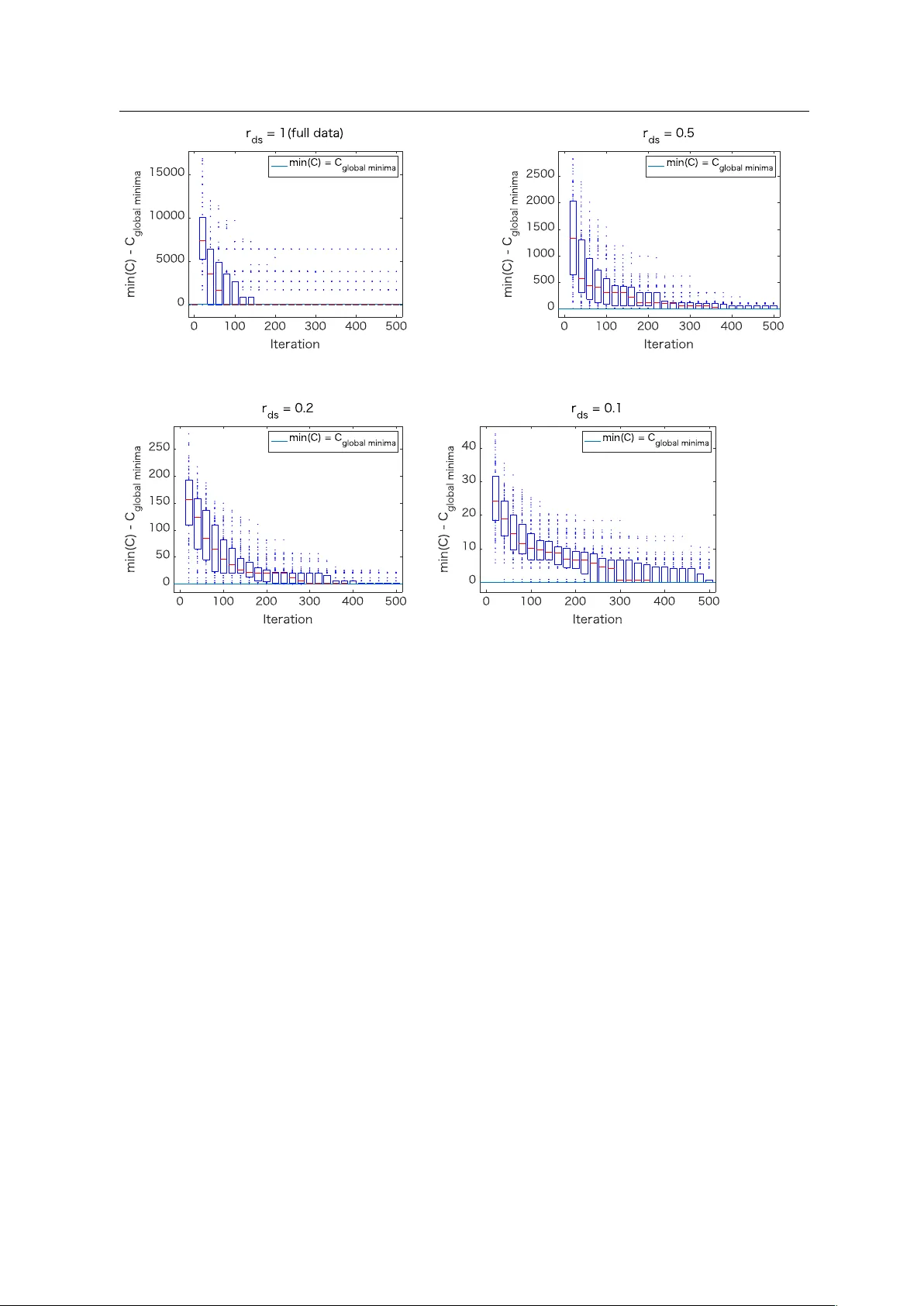
Journal of the Physical Society of Japan FULL P APERS A utomatic T ermination Strategy of Inelastic Neutr on-scattering Measur ement Using Bayesian Optimization f or Bin-width Selection K ensuke Muto 1 , 4 , Hirotaka Sakamoto 1 , K enji Nagata 2 , T aka-hisa Arima 3 , and Masato Okada 2 , 3 * 1 Graduate School of F r ontier Sciences, The University of T okyo, Chiba 277–0882, Japan 2 Resear c h and Services Division of Materials Data and Inte grated System, National Institute for Materials Science, Tsukuba, Ibaraki 305–0047, J apan 3 Graduate School of F r ontier Sciences, The University of T okyo, Chiba 277–8561, Japan 4 Karakuri, Inc., 2-7-3 Tsukiji, Chuo-ku, T okyo 104-0045, J apan Currently , an excessi ve amount of e vent data is being obtained in four-dimensional inelastic neutron-scattering experiments. A method for automatic bin-width optimization of multidi- mensional histograms has been de veloped and recently validated on real inelastic neutron- scattering data. Ho we ver , measuring be yond the equipment resolution leads to ine ffi cient use of valuable beam time. T o impro ve experimental e ffi cienc y , an automatic termination strate gy is essential. W e propose a Bayesian-optimization-based method to compute stopping criteria and determine whether to continue or terminate the experiment in real time. In the proposed method, the bin-width optimization is performed using Bayesian optimization to e ffi ciently compute the optimal bin widths. The experiment is terminated when the optimal bin widths become smaller than the target resolutions. In numerical e xperiments using real inelastic neutron-scattering data, the optimal bin widths decrease as the number of ev ents increases. Even the optimal bin widths for data downsampled to 1 / 5 are comparable with the resolu- tions limited by the sample size, choppers, and so on. This implies excessiv e measurement of the inelastic neutron experiments for the moment. Moreover , we found that Bayesian op- timization can reduce the search cost to approximately 10% of an exhausti ve search in our numerical experiments. * okada@edu.k.u-tokyo.ac.jp 1 / 14 J. Phys. Soc. Jpn. FULL P APERS 1. Introduction Inelastic neutron-scattering is an e xperimental method for in v estigating the dynamical structure of materials. 1) In recent years, numerous ev ent data have been obtained in inelas- tic neutron-scattering experiments using high-po wer accelerator-based neutron sources such as those of ISIS, 2) SNS, 3) J-P ARC, 4) and CSNS. 5) A time-of-flight neutron spectrometer designed for inelastic scattering measurements, such as MAPS, 6) MERLIN, 7) HYSPEC, 8) ARCS, 9) 4SEASONS, 10) AMA TERAS, 11) and HRC, 12) produces a large-scale ev ent data. Re- searchers obtain e vent data mapped on the four-dimensional (4D) space of transferred energy ( E ) and momentum ( q ). At present, researchers create histograms from the obtained ev ent data and analyze them. 13) It is necessary to set the bin widths when creating a histogram. Shimazaki and Shinomoto proposed a one-dimensional histogram bin-width optimiza- tion method based on minimizing a cost function, originally de veloped for neuronal spike trains in neuroscience. 14) They also proposed an extrapolation theory to predict how optimal bin width changes as the number of trials increases. This extrapolation theory provides a practical way to estimate ho w many additional experimental trials are needed to construct a meaningful histogram with su ffi cient resolution. Muto et al. extended this approach to mul- tidimensional histograms by using summed-area tables (SA T). 15, 16) The SA T implementation substantially reduces the computational cost of ev aluating the cost function for multidimen- sional histograms. Recently , T atsumi et al. applied this bin-width optimization method to real inelastic neutron-scattering data and v alidated both the optimization method and the e xtrapo- lation theory for Cu single crystal measurements at J-P ARC. 17) A practical application of multidimensional bin-width optimization is to determine whether to stop or to continue the experiment. By using a larger amount of data, we can extract more detailed features of the target materials. Howe ver , measuring be yond the reso- lution of the measurement equipment leads to ine ffi cient use of v aluable beam time. While the extrapolation theory predicts how optimal bin widths change with data size, it cannot exactly predict the optimal bin widths for each specific measurement; thus, accurate stop- ping decisions require real-time bin-width optimization during the experiment. T atsumi et al. demonstrated that parallel computation on a 32-core Xeon processor enabled such real-time optimization. 17) Ho we ver , parallel computation infrastructure requires significant operational resources. W e propose a Bayesian-optimization-based method to compute the stopping cri- teria and determine whether to stop or continue the experiment in real time. The flowchart of the method is sho wn in Fig. 1. By using Bayesian optimization to e ffi ciently search for 2 / 14 J. Phys. Soc. Jpn. FULL P APERS optimal bin widths, our approach achiev es real-time performance without requiring parallel- computation infrastructure. The experiment is terminated when the optimal bin widths be- come smaller than the expected resolutions. W e conducted numerical experiments using real experimental data and found that the optimal bin widths decrease as the number of data in- creases, which is consistent with previous studies. 14, 15, 17) Moreov er , we found that Bayesian optimization can reduce the search cost to approximately 10% of e xhausti ve search in our nu- merical experiments. This computational e ffi ciency demonstrates that our approach can serve as a practical stopping criterion for routine inelastic neutron-scattering experiments. The structure of this paper is as follo ws. In Section 2, we formulate a method of mul- tidimensional bin-width optimization and Bayesian optimization. In Section 3, we present the numerical experiments using some real experimental data to explain the significance of studying a stopping strategy and e ffi ciency of Bayesian optimization. W e discuss the results in Section 4 and provide conclusions in Section 5. 2. I m por t dat a at t im e 𝑡 . 3. Com put e opt im al bin widt h 𝚫 !" # $ = (Δ % $ , Δ & $ , Δ ' $ , Δ ( $ ) , ( Real - ti me b i n -w id th o pti mizatio n ) 1 . Se t t arg e t re sol u tio n val u es 𝚫 )* + ! , = Δ % , Δ & , Δ ' , Δ ( of t he me asu re me nt, time st e p Δ𝑡 , fo r th e b i n -w i dth op t i miza tio n ; t = Δ𝑡 . Δ - > Δ - $ . / 0 1 0 23 Tr u e F a lse Te rm i n a te 𝑡 = 𝑡 + Δ𝑡 Fig. 1. Overvie w of the termination strategy . 3 / 14 J. Phys. Soc. Jpn. FULL P APERS 2. Method 2.1 Bin-width optimization for one-dimensional e vent data Shimazaki and Shinomoto proposed a bin-width optimization method for 1D data. 14) They considered a case where researchers obtain n pieces of e vent data t i ∈ [0 , T ] (1 ≤ i ≤ n ) in the observ ation time interv al [0 , T ] and the data follow a true probability density λ ( t ). The performance of the estimator ˆ λ ( t ) for λ ( t ) can be e v aluated using the mean integrated squared error (MISE) as follo ws, MISE = 1 T Z T 0 E   ˆ λ ( t ) − λ ( t )  2  d t . (1) In statistics, MISE is used for density estimations. 18) Here, E [ · ] represents the expectation ov er di ff erent realizations of ev ent data giv en by λ ( t ). When the observ ation interv al is equally di vided into N parts, the estimator ˆ λ ( t ) is limited to the form of the histogram of the bin width ∆ = T N . A cost function is deri v ed by extracting the terms depending on the bin width ∆ from the right side of Eq. (1), as ˆ C ( ∆ ) = 2 ¯ k − v ∆ 2 , (2) where ¯ k = n N , v = 1 N N X i = 1 ( k i − ¯ k ) 2 . (3) Here, k i represents the number of ev ents contained in the i − th bin. W e define the optimal bin width as the bin width that minimizes the cost function. 2.2 Multidimensionalization of the bin-width optimization algorithm W e will consider a case where researchers obtain n pieces of event data mapped on R d . T o make a histogram, we divide the observ ation area equally into N d -dimensional rectangular parallelepipeds with bin widths ∆ 1 , ∆ 2 , . . . , ∆ d . Similarly to the 1D case, we can compute the cost function ˆ C n ( ∆ 1 , ∆ 2 , . . . , ∆ d ) as ˆ C ( ∆ 1 , ∆ 2 , ..., ∆ d ) = 2 ¯ k − v ( ∆ 1 ∆ 2 ... ∆ d ) 2 , (4) where ¯ k = n N , v = 1 N N X i = 1 ( k i − ¯ k ) 2 , (5) where k i represents the number of ev ents contained in the i − th bin. The estimator of the height of the i − th bin is ˆ θ i = k i n ∆ 1 ∆ 2 ... ∆ d . Moreover , in the multidimensional case, optimal bin widths minimize the cost function. The computational cost of calculating the optimal bin widths increases as the dimension d increases, and therefore it is essential to reduce the cost. Using the summed-area table (SA T) 4 / 14 J. Phys. Soc. Jpn. FULL P APERS algorithm, as shown in Fig. 2 for d = 2, we can reduce the computational complexity for the number of counts in each bin. 16) T o apply the SA T algorithm, it is necessary to obtain e vent data in a su ffi ciently fine histogram. The steps of SA T are shown in Algorithm 1. Since it is ! " # $ %& % ' ( $ )& % ( $ %& ) * $ )& ) 2. Compute cumulative sum $ "& + 3-1. Set the bin widths , ) & , - 3- 2. Compute the number of counts in . th bin $ " & + # / / 0 1 & 2 + 234 " 134 1. Compute “raw” count data 0 "& + , 1" 2- , 1" 2) 0 4& ) 0 4& 4 … 0 )& 4 0 )& ) … 0 "& + , 1" 2- , 1" 2) $ 4& ) $ 4& 4 … $ )& 4 $ )& ) … $ " & + , - , ) $ )& ) $ %& ) $ %& % $ )& % (If . th bin is represented as the gray area) $ )& ) $ )& % $ %& ) $ %& % ( * ( # ! " Fig. 2. Overvie w of the summed-area tables algorithm for the 2D case. W e set a su ffi cient fine histogram and call it “raw” count data a i , j . not necessary for the termination strategy to find the exact optimal bin widths, we consider only multiples of the minimum units of bin widths. It is su ffi cient to set the maximum value of ∆ i to being se veral times as lar ge as the required resolution. Let us discuss the computational complexity of the bin-width optimization. Denote the maximum di vision number in the i − th dimension as N ma x , i . Let N i be the number of axial di visions in the i − th dimension, and consider the case where the cost function is computed by setting N i from 2 to N ma x , i . Then, the computational cost of the bin-width optimization is O ( Q d i = 1 N ma x , i log N ma x , i ). 2.3 Bayesian optimization Bayesian optimization is a method for solving optimization problems in volving an objec- ti ve function. Moreov er , a Gaussian process (GP) is often used to interpolate the objectiv e function by using correlation based on the distance between the observ ation points. Bayesian optimization uses the results of the interpolation to select the next point to maximize the acquisition function. Here, we treat the e xpected impro vement (EI) 19) as the acquisition func- 5 / 14 J. Phys. Soc. Jpn. FULL P APERS Algorithm 1 Bin-width optimization (multidimensional case) Step 1: Set the minimum units of the bin widths: ∆ min , 1 , ∆ min , 2 , ..., ∆ min , d and compute “raw” count data as shown in Fig. 2(a). Compute the cumulati ve sum A i 1 , i 2 ,..., i d of the “raw” count data for preparation of the SA T algorithm. Step 2: Set the bin widths ( ∆ 1 , ∆ 2 , ..., ∆ d ). Compute the number of counts k i in the i − th bin by using the SA T algorithm. Then, compute v defined in Eq. (5). Compute ˆ C ( ∆ ) defined in Eq. (4). Step 3: Repeat step 2 to find the bin width ∆ that minimizes ˆ C ( ∆ ), and let this be the optimal bin width. tion: E I ( x ) =            ( f ∗ − µ ( x )) Φ  f ∗ − µ ( x ) σ ( x )  + σ ( x ) ϕ  f ∗ − µ ( x ) σ ( x )  , ( σ ( x ) > 0) 0 . ( σ ( x ) = 0) (6) µ ( x ) and σ ( x ) are the mean and variance functions of the Gaussian process at point x , re- specti vely , and f ∗ is the minimum v alue among the observed data. ϕ and Φ represent the normalized Gaussian function and its cumulativ e distrib ution function. EI has been proven to hav e con v ergence properties. 20) The computational complexity of the acquisition function is O ( N 2 ) when the hyperparameter (HP) of GP is fix ed, and O ( N 3 ) when the HP of GP is tuned sequentially . Here, N represents the number of searched points. 3. Results W e performed numerical experiments with experimental data to verify the v alidity of the proposed method. The data consisted of inelastic neutron-scattering measurements on Ba 3 Fe 2 O 5 Cl 2 . The unit cell of this material is body-centered cubic with a lattice constant of 9 . 96Å. 21) First, we computed the cost function for the whole experimental data and found the optimal bin widths. Then, we conducted do wnsampling to v ary the number of e v ents and computed the cost function for each downsampled data. Then, we examined the relationship between the number of ev ents and the optimal bin widths. Finally , we e xamined the e ff ecti ve- ness of BO in finding the optimal bin widths. The resolution of the experimental equipment was ∆ resol = (5 , 0 . 25 , 0 . 25 , 0 . 30)[meV , r . l . u ., r . l . u ., r . l . u . ]. 6 / 14 J. Phys. Soc. Jpn. FULL P APERS (a) (b) (c) Fig. 3. 2D slices of 4D inelastic neutron-scattering count data. Reg arding (a), q y and q z are fixed at 0 . 4845 ± 0 . 0323 and 0 . 0323 ± 0 . 0323, respectiv ely . Regarding (b), q x and q z are fixed at 0 . 6137 ± 0 . 0323 and 0 . 6137 ± 0 . 0323, respecti vely . Re garding (c), E and q y are fixed at 1 . 75 ± 0 . 25 and 0 . 6137 ± 0 . 0323, respecti vely . The upper bound of the color axes is set to 2. 3.1 Bin-width optimization for experimental data W e experimented with inelastic neutron-scattering data within 15 [meV] ≤ E ≤ 50 [meV] and momentum components 0 ≤ q x , q y , q z , in which there were 1 , 679 , 542 e vents. T o use the SA T algorithm, we set the minimum units of the bin widths in the energy and momentum directions as ∆ min , E = 0 . 5 [meV] and ∆ min , q = 0 . 13 [r . l . u . ], respectively . W e limited the search area for the optimal bin widths to multiples of the minimum unit. Since we do not consider the case where the number of ev ents is extremely small, we limit the search space of the bin width up to 10 times the minimum unit in each dimension. Since we considered a 4D space, there were a total of 10 , 000 search candidates. T o simulate the process of increas- ing data while conducting a measurement, we generated data downsampled at a rate of r d s from the full data. W e computed the cost functions for r d s = 0 . 1 , 0 . 2 , 0 . 5 , 1. Fig. 3 shows 2D slices of the 4D data. T o visualize the relation between the number of ev ents and the optimal bin widths, we plotted the one-dimensional profile of the cost functions (Fig. 4). T o unify the scale of the cost functions for di ff erent data sizes, we di vided each cost function by the square of the number of ev ents. The optimal bin widths ( ∆ E , ∆ q x , ∆ q y , ∆ q z ) [meV , r . l . u ., r . l . u ., r . l . u . ] were (4 , 0 . 32 , 0 . 26 , 0 . 32), (4 , 0 . 19 , 0 . 13 , 0 . 32), (3 , 0 . 13 , 0 . 13 , 0 . 19), and (2 , 0 . 13 , 0 . 13 , 0 . 13) for r d s = 0.1, 0.2, 0.5, and 1, respecti vely . The optimal ener gy bin width for r d s = 0 . 1 was smaller than the energy resolution of the e xperiment ∆ resol , E . 3.2 Sear c hing for the optimal bin width by using Bayesian optimization W e carried out numerical experiments to verify the e ffi ciency of BO in searching for optimal bin widths in which we applied BO to the cost functions for the do wnsampled data. 7 / 14 J. Phys. Soc. Jpn. FULL P APERS (a) (b) (c) (d) Fig. 4. 1D slices of 4D cost functions computed by changing the downsampling rate of r d s . T o unify the scale, each cost function is di vided by the square of the number of ev ents. (a)–(d) represent landscapes of the cost functions in the E , q x , q y , and q z direction. The cost value in one axis direction is visualized, and the other three axis directions are fixed to the optimal bin width. The optimal bin widths ( ∆ E , ∆ q x , ∆ q y , ∆ q z ) are (4[meV] , 0 . 32 , 0 . 26 , 0 . 32) for r d s = 0 . 1, (4[meV] , 0 . 19 , 0 . 13 , 0 . 32) for r d s = 0 . 2, (3[meV] , 0 . 13 , 0 . 13 , 0 . 19) for r d s = 0 . 5, and (2[meV] , 0 . 13 , 0 . 13 , 0 . 13) for r d s = 1. Approximate optimal bin widths and the experiment’ s resolutions are represented as filled circles and dashed lines. W e performed 100 e xperiments for each r d s with di ff erent initial ( ∆ E , ∆ q x , ∆ qy , ∆ qz ) points. W e used MA TLAB’ s bayesopt function and set the acquisition function to EI + . The results of the numerical experiments are visualized in Fig. 5. Moreov er , we estimated the computational complexity of the BO search and compared its computational cost with that of the 10 , 000 point search. For estimating the computational cost, we computed the sum of the number of di visions for each ∆ . The results are sho wn in Fig. 6. 8 / 14 J. Phys. Soc. Jpn. FULL P APERS (a) (b) (c) (d) Fig. 5. Performance of BO search in bin width selection for each r d s . The predictiv e distribution of GP was used to compute the acquisition function. 100 e xperiments were performed on the same ev ent datasets with di ff erent initial ( ∆ E , ∆ q x , ∆ qy , ∆ qz ) points. The distribution of minimum values of the cost function min ( C ) for each e xperiment is plotted as a function of the iteration number . Here, the baseline is set to the global minimum of the cost function C global minima . Box plotlines show 25th, median, and 75th percentile from the bottom of the box to top. Whisker length is set to 0. Data points outside the boxes are plotted as dots. 4. Discussion Fig. 4 indicates that the optimal bin widths decrease as the number of data increases, which is in agreement with previous studies. 14, 15, 17) This trend is consistent with T atsumi et al. ’ s findings for Cu single crystal, confirming the general applicability of the bin-width optimization theory across di ff erent material systems. The optimal bin widths for data do wn- sampled to 1 / 5 ( r d s = 0.2) are comparable with the resolutions determined by experimental conditions such as the sample size and the chopper timing. This implies that the measure- ment had some redundancy . Therefore, the dev elopment of a real-time termination strategy can help to pre vent e xcessi ve measurement. 9 / 14 J. Phys. Soc. Jpn. FULL P APERS Iteration 0 100 200 300 400 500 600 700 800 cost BO / cost 10,000 0 0.05 0.1 0.15 0.2 0.25 trial1 trial2 trial3 BO Fig. 6. Comparison of computational costs of the BO search ( co st BO ) with that of an exhausti v e search of all 10 , 000 points ( co st 10 , 000 ) for three sample numerical experiments by referring to the sequence of searched points. “BO” represents the computational cost of the acquisition function calculation only . trial 1-3 include both acquisition function computation time and cost function e v aluation. At 500 iterations, trial 1, trial 2, and trial 3 reached 10.9%, 9.3%, and 10.2% respectiv ely . It took about 3.9 hours to conduct an e xhausti ve search of 10 , 000 points. (CPU: Apple M1 Max; memory: 32 GB). It is crucial to reduce the computational complexity of the bin-width optimization in the real-time strategy . While T atsumi et al. achiev ed real-time optimization by performing a par- allel computation on a 32-core Xeon processor , 17) our Bayesian optimization approach could search e ffi ciently without requiring such a parallel infrastructure. Fig. 4 suggests that the land- scapes of the cost functions would be smooth. Since GP is e ff ectiv e in interpolating on smooth functions, we e xpect that BO will work properly . When there was a lot of data, the landscape of the cost function (Fig. 4) around the global minima seemed to be deep. Therefore, BO for bin-width optimization should be satisfactory in cases with a large amount of data. In fact, Fig. 5 shows that BO is especially e ff ectiv e for searching for the optimal bin widths when the number of data is lar ge. Note that we limited the bin-width search space to being a discrete one in this experiment, resulting in min ( C ) values in the figure ha ving a discrete structure. In our numerical e xperiments, it seemed reasonable to set the maximum number of iterations to 500 (Fig. 5). According to Fig. 6, 500 iterations of trial searches cost only about 10% of the exhausti v e 10 , 000 points search. This significant computational cost reduction demonstrates that BO-based bin-width optimization can achiev e real-time performance on standard com- puting en vironments without parallel infrastructure. Moreo ver , in “trial2”, the computational 10 / 14 J. Phys. Soc. Jpn. FULL P APERS cost significantly increased for iterations between 500 and 550. This was due to an intensiv e exploration of the small bin-width area. 5. Conclusion T o prev ent redundant measurements in inelastic neutron-scattering experiments, we pro- posed a Bayesian-optimization-based automatic termination strategy for real-time bin-width optimization. The experiment is terminated when the optimal bin widths become smaller than the target resolutions. Through numerical experiments, we demonstrated that this Bayesian optimization can reduce the search cost to approximately 10% of an exhausti v e search. By us- ing Bayesian optimization to e ffi ciently search for optimal bin widths, our approach achie ves real-time performance without requiring parallel computation infrastructure. Numerical ex- periments using Ba 3 Fe 2 O 5 Cl 2 data confirmed that optimal bin widths decrease as data accu- mulates. Even the optimal bin widths for data downsampled to 1 / 5 were comparable with equipment-limited resolutions, indicating measurement redundancy . This computational e ffi - ciency demonstrates that our approach can serve as a practical stopping criterion for routine inelastic neutron-scattering experiments, ev en on standard single-core computing en viron- ments. Acknowledgment The authors thank N. Abe, T . Omi, K. Matsuura, K. Ik euchi, R. Kajimoto, and Y . Inamura for providing us the inelastic neutron-scattering data and the e xperimental resolutions. This work was partially supported by JSPS KAKENHI Grant-in-Aid for Scientific Research(A) (No. 18H04106), No. JP19H05826, and JST CREST (JPMJCR1761). The inelastic neutron- scattering data of Ba 3 Fe 2 O 5 Cl 2 were obtained by a chopper spectrometer 4SEASONS in- stalled on BL01, J-P ARC MLF , Japan, under the proposal No. 2016A0088. A ppendix: Gaussian process Suppose that we hav e a training data set D n of n observations, D n = { ( x i , y i ) } n i = 1 , where x i denotes an input vector of dimension D , and y i denotes a scalar output. The column input vectors for all n cases are aggregated in the D × n design matrix X : = ( x 1 , ..., x n ). W e assume that each observation is the sum of the objectiv e function f , and independent identically distributed Gaussian noise ϵ y i = f ( x i ) + ϵ , (A·1) ϵ i . i . d . ∼ N (0 , σ 2 ) . (A·2) 11 / 14 J. Phys. Soc. Jpn. FULL P APERS W e assume that the joint distribution of the observ ations y and a test output f ∗ at test input x ∗ can be described as          y f ∗          ∼ N          0 ,          K ( X , X ) + σ 2 I k ( X , x ∗ ) k ( x ∗ , X ) k ( x ∗ , x ∗ )                   . (A·3) Here, k denotes a kernel function and K ( X , X ) i , j : = k ( x i , x j ). W e can analytically calculate the distribution that f ∗ | y follows. f ∗ | y ∼ N (E[ f ∗ ] , V[ f ∗ ]) , (A·4) E[ f ∗ ] = k ( X , x ∗ ) T ( K ( X , X ) + σ 2 I ) − 1 y , (A·5) V[ f ∗ ] = k ( x ∗ , x ∗ ) − k ( X , x ∗ ) T ( K ( X , X ) + σ 2 I ) − 1 k ( X , x ∗ ) . (A·6) 12 / 14 J. Phys. Soc. Jpn. FULL P APERS References 1) S. W . Lo vese y: Theory of Neutr on Scattering fr om Condensed Matter (Clarendon Press, Oxford, 1984), V ol. 1. 2) J. Thomason: Nuclear Instruments and Methods in Physics Research Section A: Accel- erators, Spectrometers, Detectors and Associated Equipment 917 (2019) 61. 3) T . Mason, D. Abernathy , I. Anderson, J. Ankner , T . Egami, G. Ehlers, A. Ekkeb us, G. Granroth, M. Hagen, K. Herwig, et al.: Physica B: Condensed Matter 385 (2006) 955. 4) H. T akada, K. Haga, M. T eshigawara, T . Aso, S.-I. Meigo, H. K ogaw a, T . Naoe, T . W akui, M. Ooi, M. Harada, et al.: Quantum Beam Science 1 (2017) 8. 5) H. Chen, Y . Chen, S. Fu, L. Ma, S. W ang, F . Chen, Y . Chen, H. Dong, L. Dong, G. Feng, et al.: Nuclear Instruments and Methods in Physics Research Section A: Accelerators, Spectrometers, Detectors and Associated Equipment (2025) 170431. 6) T . G. Perring, A. D. T aylor , R. Osborn, D. M. Paul, A. T . Boothroyd, and G. Aeppli: Pro- ceedings of the 12th Meeting of the International Collaboration on Adv anced Neutron Sources (ICANS-XII), 1994, pp. 1–60. RAL Report 94-025. 7) R. I. Be wley , R. S. Eccleston, K. A. McEwen, S. M. Hayden, M. T . Dove, S. M. Ben- nington, J. R. Treadgold, and R. L. S. Coleman: Physica B: Condensed Matter 385–386 (2006) 1029. 8) B. Winn, U. Filges, V . O. Garlea, M. Gra ves-Brook, M. Hagen, C. Jiang, M. Kenzel- mann, L. Passell, S. M. Shapiro, X. T ong, et al.: EPJ W eb of Conferences 83 (2015) 03017. 9) D. L. Abernathy , M. B. Stone, M. J. Loguillo, M. S. Lucas, O. Delaire, X. T ang, J. Y . Y . Lin, and B. Fultz: Re vie w of Scientific Instruments 83 (2012) 015114. 10) R. Kajimoto, M. Nakamura, Y . Inamura, F . Mizuno, K. Nakajima, S. Ohira-Kawamura, T . Y okoo, T . Nakatani, R. Maruyama, K. Soyama, et al.: Journal of the Physical Society of Japan 80 (2011) SB025. 11) K. Nakajima, S. Ohira-Kawamura, T . Kikuchi, M. Nakamura, R. Kajimoto, Y . Inamura, N. T akahashi, K. Aizawa, K. Suzuya, K. Shibata, et al.: Journal of the Physical Society of Japan 80 (2011) SB028. 12) S. Itoh, T . Y okoo, S. Satoh, S. Y ano, D. Kawana, J. Suzuki, and T . J. Sato: Nuclear Instruments and Methods in Physics Research Section A: Accelerators, Spectrometers, Detectors and Associated Equipment 631 (2011) 90. 13 / 14 J. Phys. Soc. Jpn. FULL P APERS 13) Y . Inamura, T . Nakatani, J. Suzuki, and T . Otomo: Journal of the Physical Society of Japan 82 (2013) SA031. 14) H. Shimazaki and S. Shinomoto: Neural Computation 19 (2007) 1503. 15) K. Muto, H. Sakamoto, K. Matsuura, T .-h. Arima, and M. Okada: Journal of the Physical Society of Japan 88 (2019) 044002. 16) F . C. Crow: Proceedings of the 11th Annual Conference on Computer Graphics and Interacti ve T echniques (SIGGRAPH ’84), 1984, pp. 207–212. 17) K. T atsumi, Y . Inamura, M. K ofu, R. Kiyanagi, and H. Shimazaki: Applied Crystallog- raphy 55 (2022) 533. 18) J. S. Marron and M. P . W and: The Annals of Statistics 20 (1992) 712. 19) J. Mockus, V . T iesis, and A. Zilinskas, The application of Bayesian methods for seeking the extremum, In L. C. W . Dixon and G. P . Szeg ˝ o (eds), T owar ds Global Optimization , V ol. 2, pp. 117–129. North-Holland, Amsterdam, 1978. 20) E. V azquez and J. Bect: Journal of Statistical Planning and Inference 140 (2010) 3088. 21) W . Leib and H. K. M ¨ uller-Buschbaum: Zeitschrift f ¨ ur Anorganische und Allgemeine Chemie 521 (1985) 51. 14 / 14