AILive Mixer: A Deep Learning based Zero Latency Automatic Music Mixer for Live Music Performances

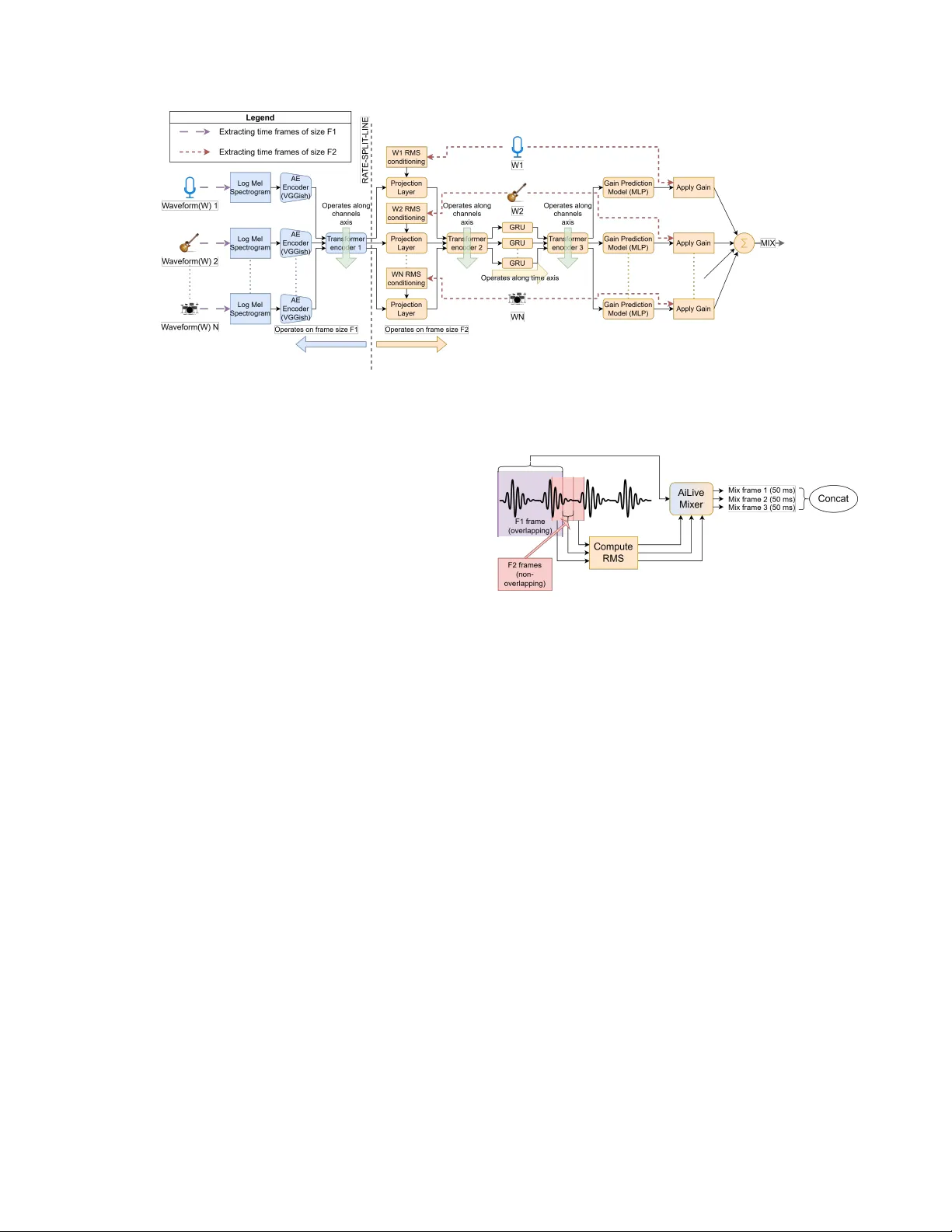
AILIVE MIXER: A DEEP LEARNING B ASED ZER O LA TENCY A UT OMA TIC MUSIC MIXER FOR LIVE MUSIC PERFORMANCES Devansh Zur ale Iris Lor ente Mic hael Lester Alex Mitc hell Shure Incorporated ABSTRA CT In this work, we present a deep learning-based automatic multitrack music mixing system catered towards li ve performances. In a liv e performance, channels are often corrupted with acoustic bleeds of co-located instruments. Moreov er , audio-visual synchronization is of critical importance thus putting a tight constraint on the audio latency . In this work we primarily tackle these two challenges of handling bleeds in the input channels to produce the music mix with zero latency . Although there have been sev eral dev elopments in the field of automatic music mixing in recent times, most or all pre vious works focus on offline production for isolated instrument signals and to the best of our kno wledge, this is the first end-to-end deep learning system dev eloped for live music performances. Our proposed system currently predicts mono gains for a multitrack input, b ut its design along with the precedent set in past works, allows for easy adaptation to future work of predicting other relev ant music mixing parameters. Index T erms — Automatic music mixing, intelligent music pro- duction, zero latency , liv e music mixing, deep learning 1. INTR ODUCTION Music mixing is an essential step in the process of producing or performing music. T ypically , a mixing engineer is responsible for processing the raw audio tracks of a musical composition, which in volv es balancing their volume lev els and applying various effects such as equalization (EQ), compression, delay , rev erb, etc. This task is inherently complex and demands substantial expertise, making it difficult for all musicians to ha ve access to qualified mixing engi- neers. Therefore, a system to automatically mix music is highly de- sired. Since the early work in [1], several traditional approaches such as [2, 3, 4] have been instrumental (pun not intended) tow ards the progress of the automatic music mixing (AMM) research. Moreo ver , with recent adv ancements in artificial intelligence (AI), se veral deep learning (DL)-based framew orks have been proposed for the AMM task. T o the best of our knowledge, most recently proposed systems are targeted to wards of fline music production. In a live music performance, instrumentalists are co-located, causing their instruments to acoustically bleed into each other’ s mi- crophones. Moreover , it is essential that the music mix is produced with minimal latency to maintain audio-visual synchronization. Al- though there is some limited work in tackling some of these chal- lenges such as in [5, 6], to the best of our knowledge no end-to-end DL-based system currently exists for AMM in a live performance setting. In this w ork we propose such a DL frame work for AMM, while focusing on the above mentioned challenges of bleeds and la- tency . A potential reason for the lack of previous research in handling bleeds is the lack of data consisting of raw multitrack corrupted with bleeds and the corresponding ground truth mixes. T o tackle this, we propose augmenting the data through parametrically simulating bleeds on data consisting of isolated instruments, which is further described in Section 3. Architecturally , a recurring theme of many previously proposed DL-based systems such as [7, 8, 9, 10] is to directly produce the mixed audio from the input multitrack. Doing so limits the users from being able to modify the generated mix, a highly desired func- tionality , gi ven the subjecti ve and artistic nature of the task. More- ov er , many of these works also expect a fixed set and order of in- struments as inputs to their models, which further limits the appli- cations of such systems. T o tackle these challenges, [11] proposed Differentiable Mixing Console (DMC), which accepts number and order in variant channel inputs to predict mix parameters of typical audio effects for every channel, thus enabling users control over the generated mix. DMC was trained for offline music production and exhibits an inherent latency of 975 ms. In this paper , we use DMC as the baseline and build upon it to enable handling of bleeds in the input channels and zero latency processing. Although DMC was trained to predict several mix parameters, in this work we only pre- dict mono gain parameters per input audio channel, thus predicting a mono gain mix. Our primary contributions in this paper are then summarized as follows: 1. W e introduce AiLi ve Mixer (ALM), a modified version of the system flow from DMC, where we propose splitting the pro- cessing into two different rates and adding feature condition- ing to better support zero latency mix prediction. 2. W e propose neural network architectural modifications such as inclusion of a transformer encoder block to learn inter- channel context and a Gated Recurrent Unit (GR U) block to learn temporal context which are aimed at better handling bleeds in the input and enabling zero latency mix prediction respectiv ely . 3. W e propose data augmentation and training strate gies to train the model in presence of bleeds 2. AILIVE MIXER SYSTEM DESIGN 2.1. Model Architectur e Fig.1 sho ws an overvie w of our proposed AiLi ve Mix er (ALM) sys- tem. In this e very raw audio channel is first passed through an audio embedding model. The extracted features are then passed through sev eral neural network blocks aimed at learning inter-channel and temporal context to predict a mono gain parameter per channel. The predicted gains for all channels are then applied to the respecti ve au- dio channel wav eform before summing together to obtain the resul- tant mono mix. All the neural network blocks share weights across Fig. 1 . AiLive Mix er - System Ov erview . Blue blocks to the left of the RA TE-SPLIT -LINE operate with a frame size of F 1 = 975 ms. Orange blocks to the right of the line operate with a frame size of F2. In MR mode, F 2 = 50 ms, in SR mode F 2 = F 1 = 975 ms. all channels and operate at one of tw o frame rates, which is further described in Section 2.2. Belo w we describe each block in detail. A udio Embedding Model: W e use a pre-trained audio embedding model to embed information pertaining to the instrument type, run- ning ov er a frame size of F 1 = 975 ms. For this we use the popular VGGish architecture [12], but more recent audio embedding mod- els such as [13, 14] could also be used here. T o enable VGGish to further embed the extent of bleeds in the respecti ve audio chan- nels, which we hypothesize is critical information required to make accurate gain predictions, we further finetune the V GGish model fol- lowing the method described in Section 4. RMS Conditioning: Most audio embedding models, including VG- Gish, are trained to be indif ferent to the amplitude of the input audio signal. The input le vel of e very channel is howev er valuable infor- mation needed to make accurate mix predictions. Thus we compute the Root Mean Square (RMS) of the input audio per F 2 frame per channel and inject it into the system using a linear projection layer followed by a PReLU acti v ation. T emporal Block (GRU): T o introduce temporal context, we use a single layer of the Gated Recurrent Unit (GR U) with a hidden size of 128 running along the temporal axis. W e hypothesize that the im- portance of temporal context is further highlighted in zero-latency processing where the model is expected to make futuristic predic- tions for the mix parameters, as further described in Section 2.3. T ransformer -encoder Blocks: The mix parameters for a giv en au- dio channel, not only depend on the channel itself, but are also ex- pected to depend on all the other channels present in the gi ven multi- track. W e use transformer-encoder blocks, which run along the chan- nels axis, to learn inter -channel conte xt using its multiheaded self- attention mechanism. W e use only a single layer of the transformer- encoder and use 2 heads per block. W e place these blocks at three different points within the system — 1. right after the audio embed- ding model, to learn context pertaining to the instrument types, 2. right after RMS conditioning, to learn context relating to the relativ e lev els of the channels and 3. right after the temporal GR U block to learn the inter-channel context of the temporally informed embed- dings. Through e xperimentation, we found that placing such dedi- cated transformers worked better than placing a single transformer- encoder with more layers at a single point in the system. Fig. 2 . Multi-Rate Processing for a single channel. Gain Prediction MLP: Finally we use a Multi-Layer Perceptron (MLP) to predict the gain parameter for ev ery channel. The MLP consists of 3 hidden layers ha ving sizes of 128 , 64 and 32 and a uni- dimensional output layer corresponding to the predicted gain. Every layer uses a PReLU activ ation function, except the final layer which uses a ReLU activ ation. 2.2. Multi-Rate (MR) Processing T o enable lo w latency processing, we split the system into two frame rates. T ypically audio embedding models require large tem- poral conte xt to embed relev ant information. Thus we extract longer frames to pass through the audio embedding model, in our case 975 ms as expected by VGGish. T ransformer-encoder 1 also operates on this frame size. Features such as RMS on the other hand, do not need such long receptive fields. Thus, we provide the capability to run the rest of the processing on shorter frame sizes, 50 ms in our case. By splitting the processing into two rates, the system can make gain predictions faster , without ha ving to w ait for the longer audio frames to become av ailable. The frame processing flow for a single channel is shown in Fig.2. In this, we first extract an F1 frame ( 975 ms) and sev eral non-overlapping F2 frames ( 50 ms). ALM then predicts gains per F2 frame, thus reducing the latency of the system to the F2 frame size. Theoretically a new F1 frame can be extracted for ev ery new F2 frame, which would mean striding the F1 frame by the size of F2 frame. Howe ver , to manage computational load, we use the same F1 frame for se veral F2 frames, before extracting a new F1 frame. For the specific case of F2 frames being 50 ms we stride the F1 frame by 6 F2 frames, which accounts to a F1 frame stride duration of 300 ms. Note that setting F2 frame size to be equal to the F1 frame size would mean that there are no rate splits. In this w ork we also pro vide results for this case in Section 6, which is referred to as Single-Rate (SR) processing. In the SR case, both F1 and F2 frames are 975 ms and non-ov erlapping. 2.3. Zero Latency Processing The proposed multi-rate (MR) processing although reduces the la- tency of the system from 975 ms to 50 ms (or lower for a lower F2 frame size), it doesn’t directly translate to zero latenc y . T o then achiev e true zero latenc y , we train our model to predict gain values for the upcoming audio. Specifically , when an F2 frame is extracted and processed, the model generates a gain prediction that is then ap- plied to the subsequent F2 time frame (one frame ahead), to obtain the predicted mix. This approach ensures that during inference, as new input audio arri ves, the model has already predicted the desired gain value for it, allowing immediate application and thereby en- abling the system to operate with genuine zero latency . Although this can theoretically be achieved without MR processing, we hy- pothesize that through MR processing the model has to only predict 50 ms into the future, as opposed to ha ving to predict 975 ms into the future, as would be the case with SR processing. This training strategy of using zero latency processing will be referred to as zero latency training. 2.4. How ALM differs from DMC DMC consists of the VGGish audio embedding model followed by concatenating the embeddings per channel with the mean of audio embeddings across channels to inject inter -channel context. These are then passed through an MLP model to predict the mix param- eters. The RMS conditioning to embed input level information, the transformer-encoders for learning the inter-channel context, the GR U for learning temporal context along with the multi-rate and zero-latency processing are what puts ALM apart from DMC. Ad- ditionally , while DMC was proposed for predicting mix parameters for offline production, ALM is trained to handle bleeds (further de- scribed in Section 3). DMC ho wev er w as also trained originally to predict mix parameters that go beyond gains, such as parameters for panning, EQ, compression, delay and re verb . In this work, we trained ALM to only predict mono gains. Howe ver , gi ven the prece- dence set by DMC, ALM could easily be extended to also predict such other mix parameters, which is left for future work. 3. TRAINING D A T A & DA T A A UGMENT A TION In this work we use MedleyDB[15, 16] to train our model, which is a dataset that consists of raw multitrack recordings and the corre- sponding human-made mixes. When it comes to liv e performances, sev eral factors gov ern the amount and kind of bleeds that e very track receiv es, such as the dimensions of the performance space, re verb lev els of the performance space, relative positions of the performers, relativ e acoustic lev els of the instruments, distance of instruments from the microphones. Collecting a dataset that encompasses suffi- cient combinations of all the abo ve factors is impractical. Thus, in this work we use isolated instrument tracks from MedleyDB and ar - tificially simulate bleeds into these ra w tracks. T o this end we built a parametric tool for bleed simulation using pyroomacoustics[17], a python library to simulate room responses. W e randomize the bleed parameters on the fly during training, thus generating a large range of bleed scenarios during training. Additionally , we also randomize the input levels for all tracks going into the system on the fly during training. This is done both after and before bleed simulation to sup- port a wide range of input lev els as well as relativ e instrument level balances respectiv ely . Giv en the impracticality of getting ground truth mixes for all bleed-simulated versions, for all such variants of a gi ven multitrack, we use as ground truth the same mix that’ s av ailable in MedleyDB, which was made for the isolated tracks. W e normalized the ground truth mixes for all songs to − 6 dB FS peak. 4. TRAINING METHODS W e used songs with < = 8 raw tracks from MedleyDB, those which consisted of isolated instruments. W e used a 80 / 20 train/v al split, thus corresponding to a total of 43 songs with 35 songs for training and 8 songs for validation. Note that although during training we used songs with isolated raw tracks with simulated bleeds, at infer- ence we use real live performances which consisted of raw tracks with naturally occurring bleeds, results for which are presented in Section 6. W e trained the model for 5000 epochs using an AdamW optimizer , where one epoch corresponds to a full pass through all the songs in the training set while randomly sampling 20 seconds snip- pets at ev ery epoch. W e started with an initial learning rate of 0 . 001 and used a multi-step learning rate scheduling, reducing the rate by a factor of 10 at epochs 100 , 1000 , 2500 . For the loss function, we use the multi-resolution STFT loss[18], using window sizes of 440 , 884 and 3528 which correspond to about 0 . 01 , 0 . 02 and 0 . 08 seconds respectively , 25% hop size for all win- dows and f ft sizes of 512 , 1024 and 4196 for each window respec- tiv ely . W e used the auraloss library[19] to compute this loss. For VGGish finetuning, we first freeze the weights of VGGish for the first 100 epochs and then unfreeze its weights, keeping the learning rates of VGGish and the rest of the model to be the same. W e found that this approach of finetuning provided the best results. 5. EXPERIMENTS T o demonstrate our contributions we trained 4 models: 1. ALM-MR (ours): Multi-Rate Processing using ALM archi- tecture trained using bleed simulations and zero latency 2. ALM-SR (ours): Single-Rate Processing using ALM archi- tecture trained using bleed simulations and zero latency 3. DMC-B-0L (hybrid): DMC model architecture, but trained using bleed simulations and zero latency 4. DMC-OG (baseline): DMC as it was proposed – using DMC architecture, trained without bleed simulations or zero latency Note: T o provide a fair comparison with ALM models, we trained both the DMC variants to only predict mono g ains. W e then ev aluated all models on multitrack recordings of liv e performances, and generating the mix es with zero latency . Addition- ally , the raw tracks that were input to these models during inference were intentionally poorly gain staged to demonstrate a novice user . Giv en the subjecti ve nature of the task, objecti ve analysis of mix quality is a challenging subject of research and no real objectiv e met- ric currently exists that is proportional to the perceptual quality of the mixes[20]. Thus we conducted a subjecti ve study to perceptually ev aluate the models. The study consisted of 15 people with critical listening skills and all working in the field of audio, including some musicians and some with a background in music mixing. Giv en Fig. 3 . V iolin + Box: Absolute Ratings that the application of this model w ould be in liv e performances, we didn’t restrict the participants to only audio engineers. W e used the W eb Audio Evaluation T ool[21] using the APE test design[22]. In this, we picked songs from an internal dataset of live performances and we played 20 − 30 s sections of e very song. 8 such se gments were used for this study . The songs were chosen to encompass dif- ferent genres of music and recorded in different scenarios. F or each song, participants were presented with mixes generated using all the 4 model v ariants along with a fifth mix – the raw mix (denoted as RA W) which was the sum of all input raw tracks. Note that to mimic a liv e mixing scenario no normalization was applied to the generated results. 6. RESUL TS & DISCUSSION T o summarize our findings from the listening test, we provide violin plots for the model ratings in Figure 3. Please also note the box plots that are embedded within the violin plots. The plots suggest that ov erall, both the ALM models outperformed the DMC models as well as the raw mix. The ratings for ALM-MR are clustered tow ards a higher rating of ∼ 0 . 75 while the ratings for DMC-OG, DMC-B- 0L and RA W are all clustered tow ards lower scores of < 0 . 5 . As for ALM-SR, the ratings are clustered higher than the DMC mod- els and RA W , howe ver the ratings are more spread out as compared to ALM-MR’ s more focused clustering in the higher ratings region. Although the difference between ALM-MR and ALM-SR might be perceiv ed as subtle, we hypothesize that ALM-MR could provide significant impro vements for the future work of predicting mix pa- rameters other than mono gain which our model currently predicts. Additionally , to demonstrate a relativ e rank, we also provide Figure 4, where the violin plots were computed for the ratings after min- max normalizing the ratings per song and per participant. Looking at the plots, the ranking could be summarized as ALM-MR > ALM- SR > DMC-B-0L > DMC-OG > RA W , which is in line with our hypothesis. T o formalize these results further, we also performed a Kruskal W allis H test[23] on the absolute ratings, which resulted in H = 156 . 485 , p = 8 . 293 × 10 − 33 , showing that there is a statistically sig- nificant difference between some of the models. W e then performed the Conover’ s test to obtain pairwise p-values for all model combi- nations. In summary , the p-v alues suggested that both ALM mod- els are statistically significantly dif ferent from the rest of the models with p values in the order of 1 × 10 − 15 - 1 × 10 − 24 . DMC-B-0L also showed statistical dif ference vs RA W . There wasn’t enough evidence to suggest significant difference between ALM-MR vs ALM-SR or DMC-OG vs DMC-B-0L or DMC-OG vs RA W . W e also provide audio results for the models at https: //dzurale.github.io/ailive_mixer_icassp2026/ . The snippets presented in these results were taken from Medle yDB Fig. 4 . V iolin + Box: Ratings normalized per song per person and consists of songs that contain naturally occurring bleeds in their raw tracks. Note that these mixes were all generated with 0 latency . 6.1. A udio Results Discussion In general, we found the DMC models to consistently e xhibit abrupt gain jumps between successive audio frames, which can be attributed to the missing temporal network in their model architecture. Even when trained with bleeds and with zero latency , the lack of the tem- poral model hampers their ability to make consistent gain predic- tions. ALM-SR also tends to exhibit some gain jumps, but far less often than the DMC models, particularly at sudden introductions of instruments. This can be attributed to the slow reaction time of ALM-SR due to its large frame size. ALM-MR almost never re- sults in any abrupt gain jumps which is also likely why it is most consistently highly rated in the listening study . This also likely ex- plains the difference between the violin plots of ALM-MR vs ALM- SR where ALM-MR is mostly concentrated around higher ratings, while ALM-SR is more spread out. ALM-MR’ s consistency was also noted by some participants through comments that we also col- lected as part of the listening study . Another finding that we’ ve heard in the model outputs is that the ALM-MR model most consistently results in mix es that are free from clipping, while the other models occasionally result in mixes that go beyond the clipping range. This is critical for systems to be used in liv e performances as normaliza- tion may not be possible. Lastly , we have also seen ALM-MR to result in better mix predictions for percussive sounds such as a bass guitar as compared to the SR models, including ALM-SR as well as the DMC models. This is likely because the ALM-MR model adapts to RMS computed ov er shorter frames, allo wing for transients in the input signals to be better modeled. 6.2. Conclusion In this paper, we introduced a system for automatic music mixing tai- lored for li ve performances, ef fectiv ely addressing track bleed issues and achie ving zero latency mix prediction. T o this end, we imple- mented a multi-rate processing strate gy (see Section 2.2) and a zero- latency processing approach (see Section 2.3) and we de veloped a bleed simulation strategy for model training (detailed in Section 3). Critical architectural enhancements to the baseline DMC model were also incorporated to facilitate these advancements, as discussed in Section 2.1. Our subjecti ve listening study and accompanying au- dio results affirm that our proposed model outperforms the baseline DMC model. Although currently focused on mono gain predictions, we anticipate that extending our ALM-MR model to predict addi- tional mix parameters will further amplify its effecti veness in future dev elopments. 7. A CKNOWLEDGEMENTS This work is based on concepts from a filed provisional patent. 8. REFERENCES [1] Dan Dugan, “ Automatic microphone mixing, ” in Audio En- gineering Society Con vention 51 . Audio Engineering Society , 1975. [2] Franc ¸ ois Pachet and Olivier Delerue, “On-the-fly multi-track mixing, ” in A udio Engineering Society Con vention 109 . Audio Engineering Society , 2000. [3] Bennett K olasinski, “ A frame work for automatic mixing using timbral similarity measures and genetic optimization, ” in A u- dio Engineering Society Con vention 124 . Audio Engineering Society , 2008. [4] Dominic W ard, Joshua D Reiss, and Cham Athwal, “Multi- track mixing using a model of loudness and partial loudness, ” in Audio Engineering Society Con vention 133 . Audio Engi- neering Society , 2012. [5] Enrique Perez-Gonzalez and Joshua Reiss, “ Automatic gain and fader control for live mixing, ” in 2009 IEEE W orkshop on Applications of Signal Pr ocessing to A udio and Acoustics . IEEE, 2009, pp. 1–4. [6] Da ve Moffat and Mark Sandler , “ Automatic mixing lev el bal- ancing enhanced through source interference identification, ” in Audio Engineering Society Con vention 146 . Audio Engineer- ing Society , 2019. [7] Marco A Martınez Ramırez and Joshua D Reiss, “Deep learn- ing and intelligent audio mixing, ” acoustic guitar , vol. 55, pp. 24, 2017. [8] M Martinez Ramirez, Daniel Stoller , and David Moffat, “ A deep learning approach to intelligent drum mixing with the wa ve-u-net, ” Journal of the A udio Engineering Society , vol. 69, no. 3, pp. 142, 2021. [9] Marco A Mart ´ ınez-Ram ´ ırez, W ei-Hsiang Liao, Giorgio Fab- bro, Stefan Uhlich, Chihiro Nagashima, and Y uki Mitsu- fuji, “ Automatic music mixing with deep learning and out- of-domain data, ” arXiv preprint , 2022. [10] Damian K osze wski, Thomas G ¨ orne, Grazina K orvel, and Bozena K ostek, “ Automatic music signal mixing system based on one-dimensional wave-u-net autoencoders, ” EURASIP Journal on Audio, Speech, and Music Processing , vol. 2023, no. 1, pp. 1, 2023. [11] Christian J Steinmetz, Jordi Pons, Santiago Pascual, and Joan Serr ` a, “ Automatic multitrack mixing with a dif ferentiable mix- ing console of neural audio effects, ” in ICASSP 2021-2021 IEEE International Conference on Acoustics, Speech and Sig- nal Pr ocessing (ICASSP) . IEEE, 2021, pp. 71–75. [12] Sha wn Hershey , Sourish Chaudhuri, Daniel PW Ellis, Jort F Gemmeke, Aren Jansen, R Channing Moore, Manoj Plakal, Devin Platt, Rif A Saurous, Bryan Seybold, et al., “Cnn ar- chitectures for large-scale audio classification, ” in 2017 ieee international conference on acoustics, speech and signal pr o- cessing (icassp) . IEEE, 2017, pp. 131–135. [13] Y uan Gong, Y u-An Chung, and James Glass, “ Ast: Audio spectrogram transformer, ” arXiv pr eprint arXiv:2104.01778 , 2021. [14] Po-Y ao Huang, Hu Xu, Juncheng Li, Alexei Baevski, Michael Auli, W ojciech Galuba, Florian Metze, and Christoph Feicht- enhofer , “Masked autoencoders that listen, ” Advances in Neu- ral Information Pr ocessing Systems , v ol. 35, pp. 28708–28720, 2022. [15] Rachel M Bittner , Justin Salamon, Mike Tierney , Matthias Mauch, Chris Cannam, and Juan P ablo Bello, “Medleydb: A multitrack dataset for annotation-intensi ve mir research., ” in Ismir , 2014, vol. 14, pp. 155–160. [16] Rachel M Bittner , Julia Wilkins, Hanna Y ip, and Juan P Bello, “Medleydb 2.0: Ne w data and a system for sustainable data collection, ” ISMIR Late Breaking and Demo P apers , v ol. 36, 2016. [17] Robin Scheibler , Eric Bezzam, and Ivan Dokmani ´ c, “Py- roomacoustics: A python package for audio room simula- tion and array processing algorithms, ” in 2018 IEEE interna- tional confer ence on acoustics, speech and signal pr ocessing (ICASSP) . IEEE, 2018, pp. 351–355. [18] Ryuichi Y amamoto, Eunwoo Song, and Jae-Min Kim, “Par- allel wav egan: A fast waveform generation model based on generativ e adversarial networks with multi-resolution spectro- gram, ” in ICASSP 2020-2020 IEEE International Confer ence on Acoustics, Speec h and Signal Processing (ICASSP) . IEEE, 2020, pp. 6199–6203. [19] Christian J. Steinmetz and Joshua D. Reiss, “auraloss: Audio focused loss functions in PyT orch, ” in Digital Music Researc h Network One-day W orkshop (DMRN+15) , 2020. [20] Christian J Steinmetz, “Learning to mix with neural audio ef- fects in the wa veform domain, ” MS thesis , 2020. [21] Nicholas Jillings, David Moffat, Brecht De Man, Joshua D Reiss, and Ryan Stables, “W eb audio evaluation tool: A frame- work for subjecti ve assessment of audio, ” 2016. [22] Brecht De Man and Joshua D Reiss, “ Ape: Audio perceptual ev aluation toolbox for matlab, ” in Audio Engineering Society Con vention 136 . Audio Engineering Society , 2014. [23] W illiam H Kruskal and W Allen W allis, “Use of ranks in one- criterion variance analysis, ” Journal of the American statistical Association , vol. 47, no. 260, pp. 583–621, 1952.