Adaptive Tube MPC: Beyond a Common Quadratically Stabilizing Feedback Gain
This paper proposes an adaptive tube framework for model predictive control (MPC) of discrete-time linear time-invariant systems subject to parametric uncertainty and additive disturbances. In contrast to conventional tube-based MPC schemes that empl…
Authors: Anchita Dey, Shubhendu Bhasin
Adaptiv e T ub e MPC: Bey ond a Common Quadratically Stabilizin g F eedbac k Gain ⋆ Anc hita Dey, Sh ubhendu B hasin Ele ctric al Engine ering Dep artment, Indian Institute of T e chnolo gy Delhi, Hauz Khas, New Delhi , Delhi 110016, Indi a Abstract This pap er prop oses an adaptive tub e framew ork for model p redictive control (MPC) of discrete-time linear time-inv ariant systems sub ject to parametric uncertaint y and additive disturbances. In contra st to conven tional tub e-based MPC schemes that emplo y fixed tub e geometry and constraint tightening designed for worst-case uncertaint y , the prop osed approach incorp orates online parameter learning to p rogressively refine the parametric uncertaint y set and up date the parameter estimates. These up dates are used to adapt the comp onents of t h e MPC optimization problem, includin g the prediction mod el, feedbac k gain, terminal set, and tub e cross-sections. As the uncertaint y set con tracts, the required amount of constrain t tigh tening redu ces and the tub e shrinks accordingly , yielding less conserv ative control actions. Recursive feasibilit y , robust constraint satisfaction, and closed-loop stability are formally established. F urthermore, the framew ork do es not require the existence of a common quadratically stabilizing linear feedback gain for the entire p arametric uncertaint y set, thereby relaxing a standard assumption in existing tub e-based MPC form ulations. Numerical examples illustrate the effectiveness of the prop osed approac h. Key wor ds: Model predictive contro l, Adaptive control, Control of constrained systems, Optimization under un certain ties. 1 In tro duction Mo del predictive control (MPC) is a n optimizatio n- based control strategy that uses a system mo del to predict future system behavior and computes an op- timal sequence of control inputs by minimizing a cost function of predicted states and inputs, sub ject to hard constraints. In the sta ndard MPC formulation, the con- strained optimal co ntrol pro blem (COCP) relies on an accurate mo del of the system dynamics for state predic- tion [1 7]. In the pr e s ence o f mo deling error s or distur - bances, howev er, the tr ue system evolution may deviate from the pre dicted tra jector ies, p o tentially lea ding to constraint viola tio ns and loss of recur sive feasibility or stability . Since ex act mo del knowledge is ra rely av ail- able in practice, the problem of desig ning MPC s chemes for systems affected by parametric uncertaint y and ad- ditive disturba nces has r e ceived considerable attention in the literature. Robust MPC metho ds ar e mostly based on either min- max optimization o r tube- ba sed approaches a nd hav e ⋆ Corresponding author A. Dey . Email addr esses: anchitadey.e e.india@gmail .com (Anchita D ey ), sbhasin@ee.iitd.a c.in (Shubhendu Bhasin). bee n extensively studied in the literature. These meth- o ds ar e t ypically desig ned for systems with kno wn pa- rameters sub ject to unknown additive disturbances [4, 20, 27], or for systems with par ametric unce rtaint y , with or without a dditiv e disturbances [3, 10, 16]. In the lat- ter case, howev er, the uncertain pa rameters are t ypically treated as unknown but fixed, a nd no mechanism is em- ploy ed to learn or refine their estimates online. T o reduce conserv atism a nd improv e p erforma nce , adaptive MPC schemes hav e recent ly been pro p o sed [9, 1 3, 1 9 , 21, 23], where the system parameter s , the se ts containing them, or b oth are up dated using online data, while predictio n error s ar e handled through ro bust tub e s. Among r obust MPC formulations, homothetic tub e MPC [20, 27] provides a conv enient parametr ized struc- ture for b ounding prediction erro rs and formulating the COCP . Conse q uent ly , recent resear ch has fo cused on reducing the conser v atism asso ciated with fixed tube constructions. F or instance, [22] prop oses a flexible tub e structure based on zonotop es, where the parameter s defining the tube cr o ss-sectio ns a r e optimized online. The framework in [18 ] considers systems with addi- tive dis turbances o nly a nd co ns tructs tub es through an online-optimized blending of o ffline-computed inv a ri- ant sets co rresp onding to different stabilizing feedback gains. Self-tuning tubes a re prop osed in [30] for sys- Preprint submitted to A utomatica 18 March 2026 tems with b o th parametric uncertaint y a nd a dditive disturbances. F or systems with parametric uncerta int y and constraints impo sed on all sta tes , most existing a ppr oaches [3, 7– 9, 13, 19 , 2 1–23, 30] assume the existence of a common quadratically stabilizing linear state feedback g ain for the entire uncerta int y set [14]. Sp e cifically , it is assumed that there ex is ts a common linear feedback gain that stabilizes the or igin of a linear time-inv a riant (L TI) s ys- tem whose sta te and input matr ices cor resp ond to any element of the pa rametric uncer taint y set. This ass ump- tion, how ever, significa ntly restricts the class of admiss i- ble uncer taint y sets [1, 11]. In g eneral, a parametric un- certaint y set may no t a dmit quadra tic stabilization, and even when quadra tic stability can be established, a lin- ear feedback gain that stabilize s every element o f the set may not exist [25]. Even in ca ses where such a common stabilizing ga in exists, the construction of a common ter- minal set satisfying the sta te and input co nstraints for all admissible systems may still b e infeasible or highly conserv ative, further restr icting the practical a pplicabil- it y of such approaches. Data-driven pre dictive control fra meworks [2, 5] provide an alternative that av oids the need for a co mmon stabi- lizing feedbac k gain. How ever, s inc e these methods rely on a n offline-cons tructed Hankel ma trix derived from previously collected data, their p er formance may de- grade if the system dy na mics changes during online op- eration. In this work, we pro p o se the no tion of adaptiv e tub es for MPC of discr ete-time L TI sy s tems sub ject to bo th parametric uncertaint y and additiv e disturbances. Spec ific a lly , we construct homothetic tub es whose cross- s ectional geometry is up dated online based on the ev olving pa rameter point estimate and the refined parametric uncertaint y set. The resulting adaptive tub e framework av o ids the co mmo n but restrictive assump- tion of the existence of a single qua dratically stabi- lizing linear feedback ga in for the en tire uncertaint y set [3, 7–9, 13, 19, 21–23, 3 0], thereby re ducing conser - v atism. T o achiev e this, the system ma tr ices ar e decomposed int o an e s timated co mpo nent and an unknown comp onent, with the la tter treated as part of a lump ed additive dis- turbance. This representation enables the formulation of a tub e-based COCP with a structure similar to that of standard ho mothetic tub e MPC [2 0, 27], while yielding improv ed c onstraint tightening thro ugh the use of sepa - rate forward r eachable disturba nce sets [4 ] ra ther than a single worst-ca se disturbance b ound. The av aila ble state and input data are used to up date bo th the pa rametric uncertaint y set [15] and the parameter po int estimate through a pro jection-mo dified nor malized gradient de- scent law [12]. The r esulting reduction in parametric uncertaint y leads to online r ecomputation of the tigh t- ened constraints, the tub e cross - sectional shap e, and the terminal set. F urthermore, the terminal ingredients are constructed using a feedback gain asso cia ted with the current parameter estimate r ather than requiring a co m- mon gain for all elements of the uncertaint y set. Al- though this a da ptation modifies the underlying COCP and may affect feasibility , r ecursive feas ibilit y is ensured by a ba ckup formulation inv oked w he n necessa ry . The prop osed scheme a lso guara n tees robust expo nential sta- bilit y [24, Def. 2] and b o undedness o f a ll signals. The main contributions of this w ork ar e t wofold. Firs t, we intro duce the notion o f a da ptive tub es for MP C of discrete-time L TI systems with parametric uncertaint y and additiv e disturbances , wher e the tube cro ss-sections , terminal set and constraint tight ening are updated on- line bas ed o n parameter learning and uncertaint y s e t contraction. Second, the prop osed framework avoids the commonly imp osed assumption of the existence of a quadratically stabilizing linear feedback ga in for the en- tire parametr ic uncertaint y set by cons tructing terminal ingredients using the current par ameter estimate. F ur - ther, we esta blish recurs ive fea sibility , ro bust exp o nen- tial stability of the origin, and b oundedness of all closed- lo op sig nals for the resulting adaptiv e tub e MPC scheme. Notations: F or tw o sets A , B ⊆ R n , the Minko wski sum A ⊕ B , { a + b | a ∈ A , b ∈ B } and a ⊕ B , { a + b | b ∈ B } , wher e a ∈ R n , the Pon tryagin differ- ence A ⊖ B , { a | a + b ∈ A ∀ b ∈ B } , the set multi- plication AB , { ab | a ∈ A , b ∈ B } , where a , b a re of conformal dimensions. The convex h ull of a ll element s in B is denoted by co ( B ). The notation W ≻ 0 ( 0) im- plies the matrix W is symmetric p o sitive-definite (pos- itive semi-definite). || · || ∞ , || · || 2 and || · || F denote ∞ -norm, 2-no rm and F ro b enius nor m, resp ectively , and || b || 2 W , b ⊤ W b for a vector b . The notatio n a i | t repre- sents the v alue o f a at time t + i predicted at time t , and ( · ) ∗ on any term denotes its optimal v alue. A se- quence { c ( p ) , c ( p + 1) , . . . , c ( q − 1 ) , c ( q ) } is repre- sented as { c ( i ) } i = p : q , and the set of all integers fro m a to b by I b a . An y signal b elonging to L ∞ implies it is bo unded. A sequence vector z t is said to b elo ng to S ( m ) if P t + k i = t z ⊺ i z i ≤ c 0 mk + c 1 ∀ t ∈ I ∞ 1 , a giv en constant m ≥ 0, a nd so me k ∈ I ∞ 1 , where c 0 , c 1 ≥ 0 [1 2, Theo- rem 4.1 1 .2]. 2 Problem Statement Consider the constraine d discrete-time L TI s ystem sub- ject to external dis turbance x t +1 = Ax t + B u t + d t , (1) x t ∈ X , u t ∈ U ∀ t ∈ I ∞ 0 , (2) 2 where x t ∈ R n , u t ∈ R m , and d t ∈ R n denote the state, input, a nd external distur bance, respectively , at time t . The disturbance d t and the system parameter ψ , h A B i ∈ R n × ( n + m ) are unknown but b elong to sets D and Ψ, resp ectively . The sets X , U a nd D are known conv ex p o lytop es containing their origins in their re s pe c- tive interiors. The set Ψ ⊆ R n × ( n + m ) is the convex hull of known vertices ψ [1] , ψ [2] , ..., ψ [ L ] , wher e L is a known finite p ositive in teger. F urther, for each ˆ ψ , h ˆ A ˆ B i ∈ Ψ, ∃ a pair ( P , K ) sp ecific to ˆ ψ such that P ≻ 0, and P − ( ˆ A + ˆ B K ) ⊤ P ( ˆ A + ˆ B K ) − Q − K ⊤ RK 0 , (3) for some given ma trices Q, R ≻ 0, where P , Q ∈ R n × n , R ∈ R m × m and K ∈ R m × n . This condition implies that each system corresp onding to ˆ ψ ∈ Ψ is stabilizable and a dmits a sta bilizing linear feedback gain K with a quadratic Lyapunov function x ⊤ P x , which is a standard assumption in MPC design [17, 20, 27]. The obje ctive is to design a suitable control u t that driv es the state of the system (1) to its origin while ens uring that the hard co ns traints (2) are satisfied despite the presence of the disturba nce d t . F or the k nown dynamics ( A and B are known) and disturba nce-free cas e, classica l approaches [17] could b e used to solve the COCP P 1 in a receding horizon fa s hion. P 1 : min µ t N − 1 X i =0 || x i | t || 2 Q + || u i | t || 2 R + || x N | t || 2 P sub ject to x 0 | t = x t , x i +1 | t = Ax i | t + B u i | t ∀ i ∈ I N − 1 0 , x i | t ∈ X , u i | t ∈ U ∀ i ∈ I N − 1 0 , x N | t ∈ X T S ⊆ X , where µ t , { u i | t } i =0: N − 1 , and X T S is the terminal set (refer to [17, Ch. 2] for details). The clas s ical COCP P 1 is not directly so lv able in the presence o f uncertainties in A , B and d t , and therefore requires refor mulation. In the subsequent sections, moti- v ated by set mem b ership-ba s ed identification [15 , 21 , 23 , 29] and homo thetic tube - based MPC metho ds [20, 27], we r eformulate the COCP us ing an adaptive tube frame- work that is designed to reduce the uncertaint y in ψ at each time instant. Due to hard constra int s on the s ystem’s states and in- puts, the adaptiv e tube framework is equipp ed with a robust fallback mechanism to ensure constra in t satisfac- tion r egardles s o f par ameter lea rning. The robust tube- based metho d serves as a bac kup if adaptation re nder s the mo dified COCP infeas ible. W e therefore s tart by de- veloping the robust fr a mework. 3 COCP com p onents wi thout adaptation A ma jor mo tiv ation for this work is to re la x the require- men t of a common quadr atically s tabilizing linear feed- back ga in for the parametric uncer taint y set Ψ, a com- mon assumption in tube-ba sed MPC frameworks for sys- tems with uncertain parameters (see [3, 7 –9, 13, 1 9, 21 – 23, 3 0]). T o this end, we rew r ite the system dyna mics in (1) a s follows. x t +1 = ˆ A t x t + ˆ B t u t + ( A − ˆ A t ) x t + ( B − ˆ B t ) u t + d t | {z } =: w t , (4) where the par ameters ˆ A t , ˆ B t are the estimates of A , B obtained at time t using a s ubsequently designed adap- tive law a nd h ˆ A t ˆ B t i belo ng to the up dated set Ψ t . The term w t acts as a lump ed additive dis tur bance. In the absence of para meter adaptation, ˆ A t = ˆ A 0 , ˆ B t = ˆ B 0 and Ψ t = Ψ 0 ∀ t ∈ I ∞ 0 , wher e Ψ 0 , Ψ. Throug hout this s e ction, we us e the suffix t for eas y extensio n to the adaptive case. 3.1 Disturb anc e set char acterization The knowledge of X , U , D , Ψ t along with ˆ A t and ˆ B t is used to character iz e the set W t containing ev ery p os sible v alue o f w t ∀ t ∈ I ∞ 0 . Define Φ t , n ξ ∈ R n × ( n + m ) ξ + h ˆ A t ˆ B t i ∈ Ψ t o , (5a) Φ A t , n ξ ∈ R n × n h ξ η i ∈ Φ t , η ∈ R n × m o , (5b) Φ B t , n ξ ∈ R n × m h η ξ i ∈ Φ t , η ∈ R n × n o . (5c) Using definitions (5b) and (5c), the set W t is g iven by W t , Φ A t X ⊕ Φ B t U ⊕ D . (6) A less conserv a tive characterization of the sets c ontain- ing w t is obtained by leveraging forward reachable sets of the state x t in the subsequent N steps 1 . A t time t , the state measurement x t is used to compute the sets for x t +1 , x t +2 , x t +3 , ..., x t + N by propaga ting the dy- namics (1). Since the sets for x t + i ∀ i ∈ I N 1 depe nd on the current state x t , w e denote these as X i,t where i is the n umber of fo r ward steps ahead of the current time t . The sets ar e construc ted recursively as follows. X 0 ,t , { x t } , (7a) X i +1 ,t , (Ψ A t X i,t ⊕ Ψ B t U ⊕ D ) ∩ X , (7b) 1 W e focus on only N steps since the sets for w t are used in constraint tightening for th e h omothetic tub e in a COCP with a prediction horizon N . 3 where Ψ A t , n ξ ∈ R n × n h ξ η i ∈ Ψ t , η ∈ R n × m o , (8a) Ψ B t , n ξ ∈ R n × m h η ξ i ∈ Ψ t , η ∈ R n × n o . (8b) W e only require X i,t ∀ i ∈ I N − 1 0 . Using (5a)-(5c), (7a)- (8b), the sets c ontaining w t + i are given by W i,t , Φ A t X i,t ⊕ Φ B t U ⊕ D ∀ i ∈ I N − 1 0 , (9) which are used to make ro bust state predictions in the MPC COCP . 3.2 T erminal set c onstruction Without adaptation, W t ≡ W 0 and W i,t ≡ W i, 0 . While W i,t contains the p o s sible v alues of w t + i ∀ i ∈ I N − 1 0 start- ing at a n y given t , the s e t W t is a sup er set of W i,t and contains the p oss ible v alues of w t + i ∀ i ∈ I ∞ 0 . W e, there- fore, use W t = W 0 to co mpute a suitable terminal set X T S t for formulating the COCP [27 ], provided the fo l- lowing s ta ndard assumption holds. Assumption 1 Given c onst r aint sets X , U , and W 0 , for e ach h ˆ A ˆ B i ∈ Ψ , with the c orr esp onding fe e db ack gain K ( ˆ A, ˆ B ) obtaine d fr om (3) , ∃ a non-empty terminal set X T S ( ˆ A, ˆ B ) such t hat X T S ⊆ X , K X T S ⊆ U , ( 10a ) ( ˆ A + ˆ B K ) X T S ⊕ W 0 ⊆ X T S , (10b) and X T S c ontains the origi n in its interior. The ideal ch oice of X T S t = X T S 0 is the maximal ad- missible RPI set satisfying (10); this can b e computed following [6 ] for ˆ A t = ˆ A 0 , ˆ B t = ˆ B 0 and K t = K 0 . Note that the terminal set X T S t along with K t obtained from (3) are sp ecific to a given parameter estimate ( ˆ A 0 , ˆ B 0 ), thereby relaxing the requir ement for a commo n pair ( P com , K com ) and a common ter minal set for all the el- ement s in Ψ, unlike [3, 7–9, 13, 19, 21– 2 3, 3 0]. Even when a common stabilizing feedback gain exists, cons tructing a common terminal set satisfying (10) for a ll a dmissible systems ca n b e difficult o r may le a d to excessive co nser- v atism. This further mo tiv ates the use of terminal ing re- dient s tailored to the current parameter estimate. 3.3 Homothetic t ub e p ar ameterization The tubes for state and control input obtained by solving the COCP at e a ch time t ar e denoted by T x t , { T x i | t } i =0: N and T u t , { T u i | t } i =0: N − 1 , (11) resp ectively . F or the ease o f so lving the CO CP , the tub e - sections in T x t are defined as T x i | t , α i | t ⊕ β i | t S t ⊆ X i,t ∀ i ∈ I N 0 , (12) where α i | t ∈ R n is the center, β i | t ≥ 0 is the sca ling factor, a nd S t determines the tub e geometry . The set S t is defined to b e the conv ex hull of user-defined v ertices s [1] t , s [2] t , ..., s [ M t ] t , where M t is finite. The state tub e- sections ca n also be expressed as T x i | t = co n z [ j ] i | t o j =1: M t , where (13a) z [ j ] i | t , α i | t + β i | t s [ j ] ∀ ( i, j, t ) ∈ I N 0 × I M t 1 × I ∞ 0 . (13b) F urther , to achiev e desirable guara ntees of stability a nd recursive fea sibility , a suitable choice of S t [7, 27 ] is tha t it co nt ains the o rigin in its in terior and is the outer RPI approximation o f the minimal RPI set sa tis fying ( ˆ A t + ˆ B t K t ) S t ⊕ W t ⊆ S t . (14) Here, K t is the feedba ck g a in obtained by s olving (3) for ˆ A t , ˆ B t , and S t can b e computed following [26]. Again, without any adaptatio n, we have S t = S 0 ∀ t ∈ I ∞ 0 . Corresp o nding to (13a), the control tub e-sections a r e written a s T u i | t , n v [ j ] i | t o j =1: M t ∀ ( i, t ) ∈ I N − 1 0 × I ∞ 0 . (15) Since the tub e-sections are expressed as co nv ex h ulls of vertices, an y p oint η ∈ T x i | t , can b e ex pressed as η = P M t j =1 τ [ j ] ( i, t ) z [ j ] i | t , where τ [ j ] ( i, t ) ∈ [0 , 1] a nd P M t j =1 τ [ j ] ( i, t ) = 1. The co rresp onding control input u as a function of η is given by the following function u = u ( η , T x i | t , T u i | t ) , M t X j =1 τ [ j ] ( i, t ) v [ j ] i | t . (16) 4 Adaptiv e tub e MPC framew ork In this section, we intro duce parameter lea rning and re- formulate the COCP with recursive feasibility and sta- bilit y guar antees. The dynamics used for developing the framework is given by (4 ) x t +1 = ˆ A t x t + ˆ B t u t + w t , where w t ∈ W t defined in (6). The suffix t w as a lready int ro duced with the estima ted para meters and sets char- acterized in the previous section to indica te their time- v ary ing nature due to ada ptation. Below, we provide the 4 laws for carry ing o ut the adaptation of the parameter estimates ˆ ψ t , h ˆ A t ˆ B t i and the uncertaint y set Ψ t . 4.1 Par ameter le arning and unc ertainty set r efinement A t eac h time step t ∈ I ∞ 1 , the av ailable data x t , x t − 1 , u t − 1 are le verage d to co mpute a non-falsified set for the true pa rameter ψ = h A B i as follows [15] Ξ t , nh ˆ A ˆ B i x t − ˆ Ax t − 1 − ˆ B u t − 1 ∈ D o . (17) The pa r ametric uncertaint y set is then up da ted a s Ψ t , Ψ t − 1 ∩ Ξ t ∀ t ∈ I ∞ 1 ; Ψ 0 = Ψ . (18) Lemma 2 F or the plant dynamics (1) , the true p ar am- eter ψ = h A B i ∈ Ψ t ∀ t ∈ I ∞ 1 , wher e t he unc ertainty sets Ψ t , obtai ne d u sing (17 ) and (18 ) , ar e neste d, i.e. , Ψ t ⊆ Ψ t − 1 ∀ t ∈ I ∞ 1 . Thi s furt her implies that Ψ t 6 = ∅ at any time t . Pr o of: The pro of ea sily follows from the plant dynamics (1) and the no n-falsified set definition in (17) and the recursive up date law (18 ), since bo th Ψ 0 and Ξ t ∀ t ∈ I ∞ 0 contain the true pa rameter ψ . Since the upda ted uncertaint y s et may yield a new set of vertices, we add a time index to the vertices of Ψ t . Ψ t = co n ψ [ i ] t o i =1: L t ∀ t ∈ I ∞ 0 , with ψ [ i ] 0 , ψ [ i ] ∀ i ∈ I L 0 1 , wher e L 0 , L. (19) Using the up dated uncertaint y set Ψ t , obtained with (18), we co mpute the p oint estimate ˆ ψ t using a no r- malized gradient descent-based law alo ng with a pro jec- tion oper ator that pro jects the e s timates o nto the un- certaint y s e t Ψ t . T o this end, w e rewr ite (1) as x t = ψ g t − 1 + d t − 1 ∀ t ∈ I ∞ 1 , (20) where g t − 1 , h x ⊤ t − 1 u ⊤ t − 1 i ⊤ ∈ R n + m . Here (20) is in a linear r egressio n form with a per turbation-like term d t − 1 , a nd at any time t , we know the terms x t and g t − 1 . Accordingly the up date la w is given by ¯ ψ t = ˆ ψ t − 1 + κ ( x t − ˆ ψ t − 1 g t − 1 ) g ⊤ t − 1 1 + g ⊤ t − 1 g t − 1 , ˆ ψ t = ( ¯ ψ t , if ¯ ψ t ∈ Ψ t arg min ξ ∈ Ψ t || ξ − ¯ ψ t || F , otherwis e , (21) where κ ∈ (0 , 2). Lemma 3 L et e t , ( x t − ˆ ψ t − 1 g t − 1 ) / (1 + g ⊤ t − 1 g t − 1 ) . The up date law in (2 1) with κ ∈ (0 , 2) guar ante es • e t , e t (1 + g ⊤ t − 1 g t − 1 ) 1 2 , ˆ ψ t ∈ L ∞ , • e t , e t (1 + g ⊤ t − 1 g t − 1 ) 1 2 , || ˆ ψ t − ˆ ψ t − 1 || F ∈ S ( ¯ d 2 ) , wher e ¯ d is the upp er b oun d of || d t (1 + g ⊤ t − 1 g t − 1 ) − 1 2 || 2 . Pr o of: The pr o of follows from [7, Lemma 1], [12, Theo- rem 4.1 1 .4] with the use o f Lemma 2. 4.2 R eformulate d COCP with adaptation Due to the adaptation of Ψ t and the par a meter esti- mate ˆ ψ t = h ˆ A t ˆ B t i , the sys tem dynamics in (4) a nd the asso ciated sets defined in (5a )-(6) a nd (7b)-(9) ar e up- dated whenever Ψ t and/or ˆ ψ t change. Accordingly , the matrices P t , K t , the terminal set X T S t and the p oly- top e S t defining the tube cross-s e c tional shap e are re- computed to re ma in co nsistent with the up dated un- certaint y desc r iption. While this introduces additional computational effort, it enables the controller to ex ploit any re duction in the size o f Ψ t , leading to the follo wing dual b enefits. • The terminal s et, which is desira bly the maximal ad- missible RPI set, increases in size, implying the need for reduced control effort to reach the terminal set, and • The tub e cros s-sectional shape S t reduces in size, al- lowing for a b etter repres e ntation o f the uncertaint y in the propaga tion o f the true state. The use of updated par ameter estimates and uncertain ty sets yields a mo dified COCP at each time instant. How- ever, the switching from the o ld setup at t − 1 to the new COCP at t with up dated ( P t , K t ) and terminal set X T S t may affect recur s ive feasibility and stabilit y . The treat- men t of fea sibility under such switc hing is discussed in the next subsection. T o ensure stability guar a ntees, we impo se certa in conditions o n the choice o f ( P t , K t ). Criterion 4 Given the p ar ameters ˆ A t , ˆ B t , the p air ( P t − 1 , K t − 1 ) and matric es Q, R , wher e Q, R, P t − 1 ≻ 0 , and c onstr aint sets X , U and W t , cho ose a p air ( P t , K t ) that satisfies P t ≻ 0 and the fol lowing c onditions. (a) P t − ( ˆ A t + ˆ B t K t ) ⊤ P t ( ˆ A t + ˆ B t K t ) − Q − K ⊤ t RK t 0 (22a) (b) P t − 1 − ( ˆ A t + ˆ B t K t ) ⊤ P t ( ˆ A t + ˆ B t K t ) − Q − K ⊤ t − 1 RK t − 1 0 , (22b) and, (c) ∃ a non-empty t erminal set X T S t such that X T S t ⊆ X , K t X T S t ⊆ U , (22c) ( ˆ A t + ˆ B t K t ) X T S t ⊕ W t ⊆ X T S t , (22d) 5 and X T S t c ontains the origin in its interior. Condition (b) plays a cruc ia l ro le in preserv ing stability under a daptation. Sp ecifically , it ens ur es that the Lya- punov function, which is ass o ciated with the cost ma- trices Q , R , and P t − 1 at time t − 1 and P t at time t , do es no t increase when the prediction mode l switches from ( ˆ A t − 1 , ˆ B t − 1 ) to ( ˆ A t , ˆ B t ) and the feedbac k gain is upda ted from K t − 1 to K t . In other words, even though the ter minal cos t a nd prediction dyna mics ar e mo dified, the v alue function remains non-incr easing along s ystem tra jectories , there by preser ving the stability guarantee across switching instances. I n the a bsence of adapta- tion, i.e., when ( ˆ A t , ˆ B t ) = ( ˆ A t − 1 , ˆ B t − 1 ), Condition (b) reduces to C o ndition (a), a nd the requirement co incides with the sta nda rd disc r ete-time Lyapuno v inequality for classical MPC [17, C h. 2]. Conditions (a) and (c) follow fro m (3) as a prop erty of Ψ 0 and Assumption 1, resp ectively . Unlike the qua dr atic stabilizability a s sumption, which requires the existence of a common pa ir ( P com , K com ) satisfying P com − ( ˆ A + ˆ B K com ) ⊤ P com ( ˆ A + ˆ B K com ) − Q − K ⊤ com RK com 0 , ∀ h ˆ A ˆ B i ∈ Ψ, to gether with a co mmon ter minal s et, Condition (b) only enfor c es a o ne-step co mpatibilit y b e- t ween conse c utive par ameter up dates . Th us, it av oids the need for a co mmon Lyapunov function and feedback gain that are v alid fo r the entire uncer taint y set. Provided Criterio n 4 holds, we compute the po lytop e S t as the outer RPI appr oximation of the minimal RPI set satisfying (14). Remark 5 If Criterion 4 do es not hold, t he p oint es- timates ˆ A t , ˆ B t and the p air ( P t , K t ) r emain unchange d. Nevertheless, adaptation may stil l o c cur thr ough c ontr ac- tion of the u n c ertainty set. The COCP for a da ptive tube MPC with decisio n v ar i- able ¯ µ t , { ( α i | t , β i | t ) } i =0: N , n v [ j ] i | t o i =0: N − 1 ,j =1: M t is given by P 2 t : min ¯ µ t M t X j =1 N − 1 X i =0 || z [ j ] i | t || 2 Q + || v [ j ] i | t || 2 R + || z [ j ] N | t || 2 P t ! (24a) sub ject to (11 ) − (13) β i | t ≥ 0 ∀ i ∈ I N 1 , (24b) T x 0 | t = { x t } , (24c) T x i | t ⊆ X , T u i | t ⊆ U ∀ i ∈ I N − 1 0 , (24d) T x N | t ⊆ X T S t ⊆ X , and (24e) ˆ A t z [ j ] i | t + ˆ B t v [ j ] i | t ∈ T x i +1 | t ⊖ W i,t ∀ ( i, j ) ∈ I N − 1 0 × I M t 1 . (24f ) Using the solution of the COCP a nd (16), w e compute the input u ∗ t = u ( x t , T x ∗ i | t , T u ∗ i | t ) that is a pplied to the plant (1) to evolve to the next state x t +1 . The COCP is lab elled as P 2 t since the formulation dep ends on time t . It is p o ssible that the new set Ψ t , with the new es- timates ˆ A t , ˆ B t and the consequently computed sets, leads to an infeasible C O CP . First, there may not exist a ( P t , K t ) that satisfies Criterio n 4. Second, even if Cr ite- rion 4 holds, (24) may be infeasible due to the inadequate length of the prediction horizon. In either case, we revert to the previous estimates by setting ˆ A t ← ˆ A t − 1 , ˆ B t ← ˆ B t − 1 , P t ← P t − 1 , K t ← K t − 1 and Ψ t ← co Ψ t , nh ˆ A t − 1 ˆ B t − 1 io , (25) and compute the sets in (5a )- (6 ), (7b)-(9), X T S t and S t . A t any time step, if there is a change in the set Ψ t or the estimates ˆ A t ˆ B t , the shap e of the disturbance-r elated sets along with the p olytop e S t changes. This r enders the tube an adap tive nature, allowing for improv ed charac- terization of the uncertainties in tr a jectory pr opagatio n of the true sys tem (1). Algorithm 1 o utlines the steps for implemen ting the prop o s ed framework. Remark 6 It is p ossible that the numb er of vertic es of Ψ t may incr e ase with t . T o ensu r e that t he appr o ach is tr actable, one c an either stop the set adaptation after the numb er of vertic es L t r e aches a pr e-de cide d upp er b ound dep ending on the c omputational r esour c es or opt for metho ds discusse d in [4, 21, 28]. Remark 7 A c c or ding to Algo rithm 1, if P 2 t is infe asible at some time t ∈ I ∞ 1 , t he COCP is re formulate d using t he setup describ e d in Steps 28 -30 and solve d with the up date d formulation. T o avoid t he additional c omputational effort asso ciate d with re solving the mo difie d pr oblem at time t , the c ontr ol input u t c an inste ad b e c ompute d us ing t he pr eviously obtaine d optima l solution at time t − 1 , to gether with the me asur e d state x t and (16) . 4.3 R e cursive F e asibili ty and Stability Analysis Next, we prove that the pr op osed CO CP P 2 t following Algorithm 1 is recur sively fea s ible, and lea ds to r o bust exp onential sta bilit y of the o rigin of (1). Theorem 8 Supp ose Assu mption 1 holds, and the COCP P 2 t is fe asible at some time t . Then, Algorithm 1 ensure s that P 2 t is fe asible at time t + k ∀ k ∈ I ∞ 1 . Pr o of: The pro of pr o ceeds by induction. Assume that the COCP is feas ible at time t . W e show fea sibility a t time t + 1 . Given a feasible solution at t , the plant (1) evolves a nd the parameter estimates , uncertaint y set and distur- 6 Algorithm 1 Adaptive T ub e MP C Input: X , U , D , ψ [ i ] ∀ i ∈ I L 0 1 , N , Q , R , ˆ ψ 0 , κ . Output: ¯ µ ∗ t ∀ t ∈ I ∞ 0 . Steps: 1: Initialize Ψ 0 = Ψ, i.e., ψ [ i ] 0 = ψ [ i ] ∀ i ∈ I L 0 1 , a con- stant c backup = 0 and time t = 0. 2: Measur e x 0 . 3: while t ≥ 0 do 4: Compute Φ t , Φ A t , Φ B t , W t , Ψ A t , Ψ B t , and X i,t , W i,t ∀ i ∈ I N − 1 0 and S t using (5a)-(9) and (14). 5: if t == 0 then 6: Cho ose P t , K t and X T S t that satisfies (3) and Assumption 1 . 7: else 8: Check if ∃ P t , K t , X T S t satisfying Cr iterion 4 . 9: if Criter ion 4 does not hold then 10: Set c backup ← 1 , t ← t − 1 and go to Step 28 . 11: end if 12: end if 13: Run the COCP P 2 t . 14: if ¯ µ ∗ t 6 = ∅ , i.e., P 2 t is fea sible the n 15: Set c backup ← 0 . 16: else 17: if t == 0 then 18: Exit the algor ithm (initially infeasible). 19: else 20: Set c backup ← 1 and t ← t − 1 . 21: end if 22: end if 23: if c backup == 0 then 24: Apply u ∗ t = u ( x t , T x ∗ i | t , T u ∗ i | t ) to the plant (1). 25: Measure x t +1 from (1). 26: Compute the non-falsified set Ξ t +1 , the uncer- taint y set Ψ t +1 , and the p oint estimate ˆ ψ t +1 using (17), (18), and (21), resp ectively . 27: end if 28: if c backup == 1 then 29: Compute Ψ t +1 using (25), and set ˆ A t +1 ← ˆ A t , ˆ B t +1 ← ˆ B t , ˆ P t +1 ← ˆ P t , ˆ K t +1 ← ˆ K t . 30: end if 31: Up date t ← t + 1. 32: end while bance sets are updated. Criterion 4 is then chec ked at t + 1. If it is satisfied, new matrices P t , K t , terminal set and tub e geometr y S t are computed, res ulting in a mo d- ified COCP . Since the problem data change, feasibility of this newly formed problem ca nno t be guaranteed a priori. If P 2 t +1 is fea s ible, the algo rithm pro cee ds with its so lution. O therwise, or if Criterion 4 do es not hold, the ba ckup setup in Step 29 is used. F o r the backup, t wo situations ar ise. (i) No u p date of p oint estimate or u nc ertainty set. In this case, the COCP coincides with the standa rd homo- thetic tub e-based MPC formulation. Recursive feasi- bilit y follows fro m the existing litera ture (see [7, 20 , 21, 27]). Let the feasible so lution at t + 1 for the non- adaptive scenario b e deno ted as follows us ing ( · ) , with ( · ) ∗ denoting the optimal solution of P t . T x 0 | t +1 = { x t +1 } , (26a) T x i | t +1 = T x ∗ i +1 | t ∀ i ∈ I N − 1 1 , (26b) T u i | t +1 = T u ∗ i +1 | t ∀ i ∈ I N − 2 0 , (26c) T x N | t +1 = α N | t +1 ⊕ β N | t +1 S t , (26d) T u N − 1 | t +1 = K t T x N − 1 | t +1 = K t T x ∗ N | t , (26e) where α N | t +1 = ( ˆ A t + ˆ B t K t ) α ∗ N | t and (26f ) β N | t +1 = min β n β ( ˆ A t + ˆ B t K t ) β ∗ N | t S t ⊕ W t ⊆ β S t o , (26g ) with z [ j ] i | t +1 and v [ j ] i | t +1 being the v ertices of T x i | t +1 ∀ i ∈ I N 0 and the ele ments of T u i | t +1 ∀ i ∈ I N − 1 0 , resp ectively , ∀ j ∈ I M t 1 . The solution is useful in pr oving r ecursive feasibility of the next case. (ii) Unc ertainty set up date only. Her e, the p o int estimates ˆ A t , ˆ B t and ( P t , K t ) remain unc hanged, while the uncertaint y set is r efined a c c ording to (25), yielding Ψ t +1 ⊆ Ψ t +1 = Ψ t . Consequently , Φ t +1 ⊆ Φ t +1 = Φ t , Φ A t +1 ⊆ Φ A t +1 = Φ A t , Φ B t +1 ⊆ Φ B t +1 = Φ B t , Ψ A t +1 ⊆ Ψ A t +1 = Ψ A t , Ψ B t +1 ⊆ Ψ B t +1 = Ψ B t , resulting in W t +1 ⊆ W t +1 = W t , S t +1 ⊆ S t +1 = S t , (27a ) X i,t +1 ⊆ X i,t +1 ⊆ X i +1 ,t ∀ i ∈ I N − 1 0 , (27b) W i,t +1 ⊆ W i,t +1 ⊆ W i +1 ,t ∀ i ∈ I N − 1 0 , (27c) X ⊇ X T S t +1 ⊇ X T S t +1 = X T S t . (27d) Leveraging (27) and the solution (26 ) for the non- adaptive cas e , we prov e that the fo llowing is a feas ible solution for the COCP a t t + 1 under the r efined sets. T x i | t +1 = α i | t +1 ⊕ β i | t +1 S t +1 ∀ i ∈ I N 0 , where (28a) α 0 | t +1 = x t +1 , β 0 | t +1 = 0 , (28b) α i | t +1 = α ∗ i +1 | t , β i | t +1 = β ∗ i +1 | t ∀ i ∈ I N − 1 1 , (28c) α N | t +1 = α N | t +1 , β N | t +1 = β N | t +1 , and (28d) T u i | t +1 = n u ( z [ j ] i | t +1 , T x i | t +1 , T u i | t +1 ) j ∈ I M t +1 1 o . (28e) It is easily seen that the centers and scaling facto r s in (28) satisfy (11)-(1 3), (24 b) a nd (24c) at t + 1 . F o r the tube- s ections, we can write T x 0 | t +1 = T x 0 | t +1 ⊆ X 1 ,t , 7 T x i | t +1 = α i | t +1 ⊕ β i | t +1 S t +1 ⊆ α ∗ i +1 | t ⊕ β ∗ i +1 | t S t = T x i | t +1 ⊆ X i +1 ,t ∀ i ∈ I N − 1 1 , T x N | t +1 = α N | t +1 ⊕ β N | t +1 S t +1 ⊆ α N | t +1 ⊕ β N | t +1 S t = T x N | t +1 ⊆ X T S t ⊆ X T S t +1 ⊆ X , co ( T u i | t +1 ) ⊆ co ( T u i | t +1 ) ⇒ T u i | t +1 ⊆ U ∀ i ∈ I N − 1 0 , which tog ether prov e the s atisfaction of (2 4d) and (24e) at time t + 1 . Finally , for (2 8 ) to satisfy (2 4f), note tha t from the non-adaptive case we hav e ˆ A t z [ j ] i | t +1 + ˆ B t v [ j ] i | t +1 ∈ T x i +1 | t +1 ⊖ W i,t +1 , S t +1 ⊆ S t +1 , T x i | t +1 ⊆ T x i | t +1 , co ( T u i | t +1 ) ⊆ co ( T u i | t +1 ), and W i,t +1 ⊆ W i,t +1 . Since the pre diction dynam- ics is linea r and the input applied to a ny z ∈ T x i | t +1 is obtained through the conv ex-combination mapping (16), it follows that ˆ A t +1 z [ j ] i | t +1 + ˆ B t +1 v [ j ] i | t +1 ∈ T x i +1 | t +1 ⊖ W i,t +1 . Hence (24f) holds at time t + 1, and the pr op osed solution in (28) s atisfies a ll the c o nstraints in P 2 t +1 . Therefore, whenever the backup setup is inv oked, a fea- sible s o lution to the COCP at time t + 1 exists . If Cr i- terion 4 is satisfied, the algor ithm instead attempts to solve the up dated pro blem P 2 t +1 corres p o nding to the mo dified pro blem data. If this problem is feasible, the re- sulting solution is applied; o therwise, the backup setup ensures feasibility . Rep eating the same argument at sub- sequent time steps establishes recurs ive feasibilit y of the prop osed MPC COCP . Corollary 9 Su pp ose Assumption 1 hold s, and t he COCP P 2 t is fe asible at time t . Then, by L emmas 2, 3 and The or em 8, it is guar ante e d t hat the signals x t , u t , ˆ ψ t ∈ L ∞ . Theorem 10 Supp ose Assumption 1 holds, and the COCP P 2 t is fe asible at time t . Then, Algo rithm 1 guar ante es r obust exp onential stability of the origin of the plant (1) . Pr o of: The pro of follows the standa rd MPC s tability argument [17] by using the cost function of the COCP as a candida te Lyapunov function. Let the COCP cost function b e denoted a s J t ( x t , ¯ µ t ) , M t X j =1 Γ [ j ] t , wher e Γ [ j ] t , N − 1 X i =0 || z [ j ] i | t || 2 Q + || v [ j ] i | t || 2 R + || z [ j ] N | t || 2 P t is the comp onent of the cos t function for eac h vertex of the tube -sections. T o address the change in the num b er of vertices ( M t to M t +1 ) due to a change in the tub e geometry , define the v a riables ρ 1 t , 0 , if M t ≤ M t +1 1 , otherwis e, ρ 2 t , 0 , if M t ≥ M t +1 1 , otherwise . Also, let γ 1 , max t ∈ I ∞ 0 ,x ∈ X ,u ∈ U N ( || x || 2 Q + || u || 2 R ) + || x || 2 P t +1 , (29) which by Lemmas 2 , 3 and Theo rem 8 is finite. A t an y time t + 1, where t ∈ I ∞ 0 , we can write J ∗ t +1 ( x t +1 ) ≤ J t +1 ( x t +1 , ¯ µ t +1 ) = M t +1 X j =1 Γ [ j ] t +1 = M t X j =1 Γ [ j ] t +1 − ρ 1 t M t X j = M t +1 +1 Γ [ j ] t +1 + ρ 2 t M t +1 X j = M t +1 Γ [ j ] t +1 ≤ M t X j =1 N − 1 X i =0 || z [ j ] i | t +1 || 2 Q + || v [ j ] i | t +1 || 2 R + || z [ j ] N | t +1 || 2 P t +1 ! + ρ 2 t ( M t +1 − M t ) γ 1 (using (29)) ≤ M t X j =1 N − 1 X i =0 || z [ j ] i | t +1 || 2 Q + || v [ j ] i | t +1 || 2 R + || z [ j ] N | t +1 || 2 P t +1 ! + ρ 2 t ( M t +1 − M t ) γ 1 ∵ T x i | t +1 ⊆ T x i | t +1 , co ( T u i | t +1 ) ⊆ co ( T u i | t +1 ) = M t X j =1 N − 2 X i =0 || z [ j ] ∗ i +1 | t || 2 Q + || v [ j ] ∗ i +1 | t || 2 R + || z [ j ] N | t +1 || 2 P t +1 + || z [ j ] ∗ N | t || 2 Q + K ⊤ t RK t ! + ρ 2 t ( M t +1 − M t ) γ 1 (using (26)) = J ∗ t ( x t ) − M t X j =1 || z [ j ] ∗ 0 | t || 2 Q + || v [ j ] ∗ 0 | t || 2 R + || z [ j ] ∗ N | t || 2 P t + M t X j =1 || ( ˆ A t +1 + ˆ B t +1 K t +1 ) z [ j ] ∗ N | t + w t + N || 2 P t +1 + || z [ j ] ∗ N | t || 2 Q + K ⊤ t RK t + ρ 2 t ( M t +1 − M t ) γ 1 8 ≤ (1 − γ 2 ) J ∗ t ( x t ) + M t X j =1 −|| z [ j ] ∗ N | t || 2 P t + || z [ j ] ∗ N | t || 2 Q + K ⊤ t RK t + || z [ j ] ∗ N | t || 2 ( ˆ A t +1 + ˆ B t +1 K t +1 ) ⊤ P t +1 ( ˆ A t +1 + ˆ B t +1 K t +1 ) + M t max t ∈ I ∞ 0 , w ∈ W t || w || 2 P t +1 + ρ 2 t ( M t +1 − M t ) γ 1 , (b y Cauch y- Sch wartz inequa lity) where P M t j =1 || z [ j ] ∗ 0 | t || 2 Q + || v [ j ] ∗ 0 | t || 2 R = γ 2 J ∗ t ( x t ), imply- ing γ 2 ∈ (0 , 1] ⇒ 1 − γ 2 ∈ [0 , 1) (by definition of J ∗ t ) . Since the COCP is initially feasible and Assumption 1 holds, by Theorem 8, re cursive feasibility is guara nteed. Either Criterion 4 is satisfied, or we revert to ˆ A t +1 = ˆ A t , ˆ B t +1 = ˆ B t , P t +1 = P t and K t +1 = K t that satisfies (3). In any case, w e hav e P t − ( ˆ A t +1 + ˆ B t +1 K t +1 ) ⊤ P t +1 ( ˆ A t +1 + ˆ B t +1 K t +1 ) − Q − K ⊤ t RK t 0 , ⇒ J ∗ t +1 ( x t +1 ) ≤ (1 − γ 2 ) J ∗ t ( x t ) + ρ 2 t ( M t +1 − M t ) γ 1 + M t max t ∈ I ∞ 0 , w ∈ W t || w || 2 P t +1 . F or implementation purp o ses, w e put an upp er limit M max on the num ber of v ertices S t , depending on the computational power. Due to recursive feasibility a nd bo unded sets D a nd Ψ t , the v alue of w t is upper b ounded. The elements of P t are a ls o upp er bo unded, since P t is inv o lved in the cost function. Ther efore, we c a n define a constant γ 3 , M max max t ∈ I ∞ 0 , w ∈ W t || w || 2 P t + ( M max − M min ) γ 1 resulting in J ∗ t +1 ( x t +1 ) ≤ (1 − γ 2 ) J ∗ t ( x t ) + γ 3 , (30) which implies the pla nt (1) exhibits r o bust expo nential stability . F urther, once the learning has conv erged, M t remains constant and the term M t +1 − M t bec omes 0, implying that the state eventually con verges to a finite set that dep ends o n the sizes of D and Ψ t and ˆ A t , ˆ B t as t → ∞ , all of whic h are b ounded (see Cor ollary 9). 5 Numerical Exampl e W e v alidate the prop ose d MPC fra mework using the fol- lowing 2 nd order L TI sy stem 2 . x t +1 = " 0 . 2 1 . 015 − 0 . 282 5 1 # x t + " 1 . 08 3 # u t + d t with || d t || ∞ ≤ 0 . 1 and constraints || x t || ∞ ≤ 20, || u t || ∞ ≤ 1 0. The para metric uncertaint y is considered 2 A 2 nd order system is c hosen for ease of visualizing the tub es. 0 5 10 15 -5 0 5 0 5 10 15 -20 0 20 Fig. 1. State and control input. 0 5 10 15 0 0.2 0.4 0.6 2 4 6 8 10 12 14 0 5 10 -3 Fig. 2. F rob en ius norm of the parameter estimation error. 0 5 10 15 2 2.1 0 5 10 15 0.2 0.3 0.4 0 5 10 15 3 3.5 0 5 10 15 -0.1 -0.05 0 0.05 0 5 10 15 -0.4 -0.39 -0.38 2 4 6 8 10 12 14 2.0285 2.029 2 4 6 8 10 12 14 0.154 0.156 2 4 6 8 10 12 14 2.915 2.92 2.925 2 4 6 8 10 12 14 -0.1 -0.099 -0.098 2 4 6 8 10 12 14 -0.3794 -0.3793 -0.3792 Fig. 3. Elements of the terminal cost weigh t matrix, and the stabilizing linear feedbac k gain. in tw o elemen ts o f A and one ele ment of B with 3 ver- tices of Ψ given by ψ [1] = h 0 . 2 1 . 3 0 . 7 ; − 1 1 3 i , ψ [2] = h 0 . 2 1 . 2 0 . 9 ; − 0 . 25 1 3 i , ψ [3] = h 0 . 2 1 1 . 1 ; 0 . 35 1 3 i . The results in Fig.s 1-8 a re provided for x 0 = [18 ; − 18], N = 10, Q = h 1 0 ; 0 1 i , R = 0 . 1 and κ = 0 . 9 with ˆ ψ 0 = ( ψ [1] + ψ [2] + ψ [3] ) / 3. It is seen from Fig. 1 that the hard constr aints in (2) are sa tisfied, and the state tra jectory con verges to the neighbourho o d of the or igin. The pa rameter estimatio n error norm is b ounded as shown in Fig . 2, and the v ari- ations in the elements o f P t and K t are shown in Fig . 3. 9 Fig. 4. Barycentric representation of th e parametric uncer- taint y sets containing the convex com bination of the t rue parameter (shown with a blue dot). Fig. 5. (a), (b ) The polytop es u sed to d efine the cross-sec- tional shap e of the homothetic tub es, (c) The terminal sets. The reduction o f the size o f the parametric uncertaint y set Ψ t at t = 1 , 3 , 11 is shown in Fig. 4 . F rom Fig. 5 (a), (b) and (c), the adaptation in the shap e of the homo- thetic tube S t and the terminal set X T S t is visible. The shap e of S t changes and the size reduces, giving a b etter characterization of state propagation in the prese nce of uncertaint y Ψ t and D , wher e as the ter minal set size in- creases thereby r educing the str a in on the controller to reach the terminal set. T o highlight the impac t of tube adaptation, the p erfor mance of the pro p o sed MPC is compared with the robust homothetic tube MPC scheme of [27]. The compar ison focuse s on the amo unt of con- straint tightening r equired to g ua rantee robustness, the stabilization p erfor mance and the ass o ciated stage cos t. Fig. 6 shows the predicted state tub es at selected time instants. The first and second subplots corres p o nd to the tubes gener ated at t = 0 and t = 1, resp ectively . The tube pro duced by the prop os ed adaptive method (shown in green) is noticeably smalle r than the tubes obtained using the robust ho mothetic tub e MPC metho d of [27] (shown with magenta o utline). This reduction in tub e size is a dire ct consequence of the contraction of the parametric uncer ta int y set throug h online lea rning. The sec ond s ubplo t further shows that the tub e gener- ated by the propo sed metho d without adaptation (blue Fig. 6. T ub es generated at t = 0 and t = 1 follo wing the prop osed framew ork and [27], along with t he state tra jectory generated with the p rop osed metho d. outline) is still smaller tha n the tube gener ated follow- ing [27]. T his is becaus e even without ada ptation, the disturbance s et characteriza tion is impro ved at each time step, whereas the robust tub e MPC scheme re lie s o n a fixed set that acco unt s for a ll admissible distur bance w t , thereby lea ding to la rger tub e cross-sec tio ns. The tightening sets ass o ciated with the disturbance bo unds a re illustra ted in Fig.s 7 (a) and (b) for t = 0 and t = 1, re sp ectively . The tigh tening set used b y the metho d of [27] is shown in grey in Fig. 7 (a ) and re- mains fixed ov er time. In co ntrast, the tightening sets generated b y the prop osed method, shown in Fig. 7 (a) and (b), shr ink a s the parametric uncer taint y set is refined thr ough learning. This reductio n enlarge s the region av ailable for the sta te tra jector y to evolve while maintaining r obust constr aint satisfac tion. The improvemen t in p erfor mance is reflected in Fig. 8. The figure shows the evolution o f the state nor m k x t k 2 and the cumulativ e stage c ost for the prop os e d metho d and the robust tube MPC scheme of [27]. The prop os e d adaptive scheme achieves a faster reduction of the sta te norm, indica ting improv ed sta bilization p er formance. In addition, the cumulativ e stage cost is low er , reflecting a r e duction in control effort enabled by the improv ed mo del r epresentation obta ined through online lear ning. These r esults demonstra te that adapting the tub e geo m- etry and other COCP co mpo nent s thro ug h online r efine- men t of the unce r taint y s et s ig nificantly reduces conser- v atism while ma int aining r o bust constraint satisfaction. 10 Fig. 7. Sets used for constraint tigh tening corresp onding to the disturbance b ounds for the prop osed adaptive metho d and the robust t ub e MPC [27]. 0 5 10 15 700 800 900 1000 1100 0 5 10 15 0 10 20 Fig. 8. Compariso n of || x t || 2 and the cumulativ e stage cost for th e prop osed method and [27] . 6 Conclusion This pap er introduce s a n adaptive tube framew ork for MPC of discre te-time L TI systems sub ject to par a- metric unce r taint y and additiv e disturbances. The ap- proach integrates ho mothetic tub e-based MPC with set-membership identification, a llowing the parametric uncertaint y set and parameter estimates to b e up dated online us ing av aila ble state and input data. As the un- certaint y set con tracts, the tube cross-sectio ns adapt according ly , leading to less conserv a tive constraint tigh t- ening and state pro pagation. It is forma lly established that the r esulting adaptive tube MPC scheme g uaran- tees recur sive feasibility , robust exp onential stability , and b oundedness o f all s ig nals, despite the time-v ar ying nature o f the COCP induced by adaptation. A key theoretical feature o f the fra mework is that it av oids the standard a ssumption of a common quadr atically stabilizing linear feedback gain for the entire paramet- ric uncertaint y set, instead req uir ing only a one- step Lyapuno v compatibility c o ndition b etw een consecutive parameter up dates. A backup mechanism e ns ures that these guar antees ar e preser ved even when the a daptive upda tes render the mo dified COCP infeasible. Numeri- cal results demons tr ate the b enefits of the adaptive tube construction in reducing conser v atism and improving per formance. F uture work will fo cus on reducing the computational burden a s so ciated with online reco mpu- tation of tube and terminal ingredient s and e xtending the fra mework to the output feedback scenar io. References [1] B Ross Bar mish. Necessary and sufficient conditions for quadratic stabilizabili t y of an uncertain system. Journal of Optimization the ory and applic ations , 46(4 ):399–408, 1985. [2] Julian Berb er ich , Johannes K¨ ohler, Matthias A M ¨ uller, and F rank A llg¨ ow er. Data-driven mo del predictive control with stability and robustness guarante es. IEEE T r ansactions on Au tomatic Contr ol , 66(4):1702– 1717, 2020. [3] Monimoy Bujarbaruah, Ugo Rosolia, Yv onne R. St¨ urz, and F rancesco Borrell i. A simple robust MPC for l inear systems with parametric and additive uncertain t y . In A meric an Contr ol Confer e nc e , pages 2108–2113, 2021. [4] L. Chisci, J.A. Rossiter, and G. Zappa. Syst ems with pers i sten t disturbances: predictive cont rol with r estricted constrain ts. Automatic a , 37(7):10 19–1028, 2001. [5] Jeremy Coulson, John Lygeros, and Florian D¨ orfler. Data- enabled predictive con trol: In the shall o ws of the DeePC. In Eur op ea n Contr ol Confer enc e , pages 307–312, 2019. [6] Anchita Dey and Sh ubhendu Bhasin. Computat ion of maximal admi ssible robust p osi tive inv arian t s ets for linear systems with parametric and additiv e uncertainties. IEEE Contr ol Systems L ett ers , 8:1775–1780, 2024. [7] Anchita Dey and Shu bhendu Bhasin. Adaptiv e output feedbac k MPC wi th guarant eed stabilit y and robustness. IEEE T r ansactions on Au tomatic Contr ol , 70(12):8345–8 352, 2025. [8] Anchita Dey , Abhishek Dhar, and Shub hendu Bhasin. Adaptiv e output feedbac k mo del predictiv e con trol. IEEE Contr ol Systems L ett ers , 7:1129–1134, 2023. [9] Abhishek Dhar and Shub hendu Bhasin. Indirect adaptiv e MPC f or discrete-time L TI systems with parametric uncertain ties. IEEE T r ansactions on Auto matic Contr ol , 66(11):549 8–5505, 2021. [10] James Fl eming, Basil Kouv aritakis, and M ark Cannon. Robust tube MPC for linear systems with multiplicativ e uncertain t y . IEEE T r ansactions on Autom atic Contr ol , 60(4):1087 –1092, 2015. [11] Pascal Gahinet and Pierre Apk ar ian. A linear matrix inequalit y approach to H ∞ con trol. International Journal of R obust and Nonline ar Contr ol , 4(4):421–448, 1994. [12] Petros Ioannou and Bari¸ s Fi dan. A daptive Contr ol Tutorial . SIAM, 2006. [13] Sh Jafari F esharaki, M Kamali, and F Sheikholeslam. Adaptiv e tube-based mo del pr edictive cont rol for l inear systems with parametric uncertaint y . IET Contr ol The ory & Applic ations , 11(17):2947– 2953, 2017. [14] Pramo d P Khargonek ar, Ian R Petersen, and K emi n Zhou. Robust stabilization of uncertain linear systems: quadratic stabilizability and H ∞ con trol theory . IEEE T r ansactions on A utomatic Contr ol , 35(3):356 –361, 1990. [15] R.L. Kosut, M.K. Lau, and S.P . Boyd. Set-membership iden tification of systems with parametric and nonparametric uncertain t y . IEEE T r ansactions on Autom atic Contr ol , 37(7):929– 941, 1992. [16] Mayuresh V. Kothare, V enk ataramanan Balakri shnan, and Manfred Morari. Robust constrained mo del predict ive control using linear matrix inequalities. A utomatic a , 32(10):1361 – 1379, 1996. 11 [17] Basil Kouv aritakis and Mark Cannon. Mo del Predictive Con trol. Cham, Switzerland: Springer International , 38, 2016. [18] Markus K¨ ogel and Rolf Findeisen. Robust MPC with r educed conserv atism blending multiples tubes. In Americ an Contro l Confer ence , pages 1949–1954, 2020. [19] Johannes K¨ ohler, Elisa Andina, Raffaele Soloperto, Matthias A. M ¨ uller, and F r ank Al lg¨ ow er. Li near robust adaptiv e model predictive cont rol: Computational complexit y and conserv atism. In IEEE Confer enc e on De cision and Contr ol , pages 1383–1 388, 2019. [20] Wilbur Langson, Ioannis Chrysso choos, SV Rak ovi ´ c, and Da vid Q M ay ne. Robust mo del predictiv e con trol using tubes. Au tomatic a , 40(1) :125–133, 2004. [21] Matthias Lorenzen, Mark Cannon, and F rank A l lg¨ ow er. Robust MPC wi th r ecursive mo del up date. Automatic a , 103:461–471 , 2019. [22] Xiaonan Lu and Mark Cannon. Robust adaptiv e tube model predictiv e control. In Americ an Contr ol Co nfer enc e , pages 3695–370 1, 2019. [23] Xiaonan Lu and Mark Cannon. Robust adaptiv e model predictiv e control with persistent excitation conditions. Au tomatic a , 152:11095 9, 2023. [24] David Q Mayne , Sa ˇ sa V Rako vi´ c, Rolf Findeisen, and F rank Allg¨ ow er. Robust output f eedbac k mo del pr edictiv e control of constrained linear systems. A utomatic a , 42(7):12 17–1222, 2006. [25] I. P etersen. Quadratic stabilizabili t y of uncertain linear systems: Existence of a nonlinear stabili zing con trol do es not i m ply existence of a linear stabilizi ng cont rol. IEEE T r ansactions on Automa tic Contr ol , 30(3):291–29 3, 1985. [26] Sasa V Rak ovic, Er i c C Ker r igan, Konstantinos I Kouramas, and David Q Mayne. In v ari an t approximations of the minimal robust positively inv ariant set. IEEE T r ansactions on A utomatic Contr ol , 50(3):406 –410, 2005. [27] Sa ˇ sa V Rak ovi ´ c, Basil Kouv ar itakis, Rolf Findeisen, and Mark Cannon. Homothe tic tub e mo del predictive control. Au tomatic a , 48(8) :1631–1638, 2012. [28] H. Messaoud S. M. V eres and Journal of P . Norton. Limited-complexit y mo del-unfalsifying adaptive tracking- con trol. International Journal of Contr ol , 72(15):1417–14 26, 1999. [29] Andr´ as Sasfi, Melanie N Zeil inger, and Johannes K¨ ohler. Robust adaptiv e MPC using con trol contraction metrics. Au tomatic a , 155:11116 9, 2023. [30] Damianos T ranos, Alessio Russo, and Alexandre Proutiere. Self-tuning tube-based m o del predictive con trol . In Americ an Contr ol Confer enc e , pages 3626–36 32, 2023. 12
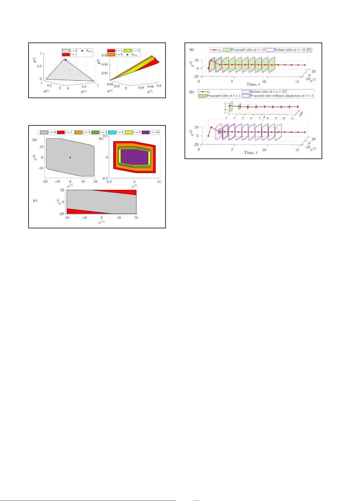
Original Paper
Loading high-quality paper...
Comments & Academic Discussion
Loading comments...
Leave a Comment