A Non-Binary Method for Finding Interpolants: Theory and Practice

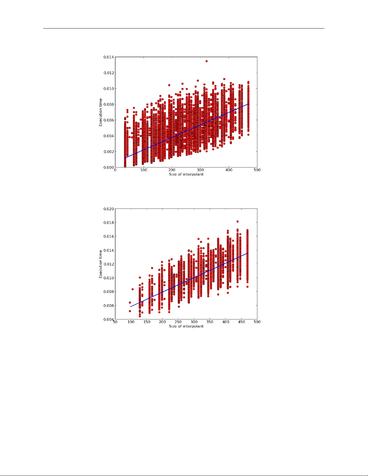
A N O N - B I N A RY M E T H O D F O R F I N D I N G I N T E R P O L A N T S : T H E O RY A N D P R AC T I C E A P R E P R I N T Adam T rybus Institute of Philosophy Jagiellonian Univ ersity 52 Grodzka St., Kraków 31-044, Poland adam.trybus@uj.edu.pl Karolina Ro ˙ zko The Univ ersity of Zielona Góra, Poland. T omasz Skura The Univ ersity of Zielona Góra, Poland. March 18, 2026 A B S T R AC T W e describe a ne w method of finding interpolants for classical logic using certain refutation system as a starting point. Refutation can be thought of as an alternati ve approach to the analysis of formal systems: instead of focusing on which formulas prov ably belong to a giv en logic, it shows which formulas are to be rejected. Thus, it pro vides a mirror proof system. As it turns out, the benefits of such an approach go well beyond the area of refutation calculi themselves. W e provide one such example in the shape of an interpolant-searching method. T o be sure, a number of such methods are already in use. The novelty of our proposal lies in the fact that it can be considered as based on a non-binary version of resolution. Keyw ords proof systems · refutation systems · interpolation · classical propositional logic 1 Introduction Our goal is twofold. First, to describe a new method of finding interpolants in classical propositional logic; and second, to demonstrate the practical applicability of this method by providing an appropriate implementation and testing i ts performance. In broad strokes, the interpolation theorem for FOL states that gi ven two formulas A and B sharing at least one predicate symbol and such that A → B is valid, there e xists a formula C (called an interpolant ) built from the predicate symbols shared by A and B , such that A → C and C → B are valid (see Craig [1957]). In case of classical propositional logic, the condition is that A and B have to share at least one propositional v ariable. The main theoretic result of this paper is a new proof of the theorem. Our approach stems from the research on the so-called r efutation systems , where the focus is on rules of r ejection of formulas. A refutation system is a collection of non-v alid formulas (refutation axioms) together with (refutation) rules preserving non-validity . This concept was introduced by Łukasiewicz in Łukasie wicz [1957] (for more on refutation systems see e.g. Skura [2011]). W e make use of such a system designed for classical propositional logic (see Skura [2013], p. 110 – 115) and sho w how it can be used in an interpolant-searching procedure. W e implement this procedure in a form of a Python script and present the results of an analysis of its performance. 2 Preliminaries W e define the syntactical and semantic notions in line with the usual practice. A Non-Binary Method for Finding Interpolants A P R E P R I N T Syntax. Lowercase letters p, q , . . . — called pr opositional variables — together with two constants ⊥ ( F alsum ) and ⊤ ( V erum ) form a set of atomic formulas ( A T ). The set FOR of well-formed formulas (the elements of which are denoted by uppercase letters A, B , . . . possibly with subscripts) is generated in a standard way from the set A T and the follo wing connectiv es: ¬ (negation); ∧ (conjunction); ∨ (disjunction); → (implication) and ≡ (equiv alence). A literal l is either a propositional variable (a positive literal) or its negation (a ne gative literal). W e call l ∗ the complement of l and define it as follo ws. If l is a positi ve literal p , then l ∗ is ¬ p and if l is a negati ve literal ¬ p , then l ∗ is p . In the remainder of the article, we assume that whenev er m , n are used, these stand for natural numbers: m , n ≥ 0 . W e denote sets (most cases, sets of formulas) in the following way: X , Y , . . . , if needs be extending this notation with subscripts. Let X = { A 1 , ..., A n } , where each A i ∈ F O R . The expression V X stands for the formula A 1 ∧ ... ∧ A n , whereas W X stands for A 1 ∨ ... ∨ A n . If X is a finite (possibly empty) set of literals, then by X ∗ we denote the set where ev ery literal of X is replaced by its complement and call V X ∗ a complement of W X and W X ∗ a complement of V X . (If X = ∅ , then W X = ⊥ with V X ∗ = ⊤ and V X = ⊤ with W X ∗ = ⊤ .) W e extend this notation in the following way: when X is a set of formulas A 1 , . . . , A n that are all either disjunctions or conjunctions of literals, then by X ∗ we mean the set containing A ∗ 1 , . . . , A ∗ n . A clause is a formula of the form W S , where S is a finite set of literals. 1 W e say that a formula A is in a conjunctive normal form (CNF), if A is of the form B 1 ∧ . . . ∧ B m , where each B i is a clause; A is in a disjunctive normal form (DNF), if A is of the form B 1 ∨ . . . ∨ B m , where each B i is the complement of a clause. W e introduce the follo wing notational con vention. Let X = { A 1 , . . . , A n } and Y = { B 1 , . . . , B m } . W e define X − → Y to be V X → W Y . W e also write A 1 , . . . , A n − → B 1 , . . . , B m , for X − → Y . Any formula of this shape with V X in CNF and W Y in DNF is said to be simply in a normal form . Finally , consider a formula V X → W Y in a normal form and put Z = X ∪ Y ∗ . Any formula of the shape Z − → ⊥ is said to be in a clausal normal form . The r ank of a (formula in a) clausal normal form is the number of literals l such that l and l ∗ occur in distinct clauses in Z . Semantics. Consider the set V of all classical valuation functions v : AT − → { 1 , 0 } (that is the functions extended to the set F O R by means of classical interpretation of the connectiv es). W e say that A is valid and write | = A , if v ( A ) = 1 for any classical v aluation function v ∈ V . The set of all valid formulas will be denoted as C L . W e recall that e very formula A can be con verted to a formula A ′ with the property | = A ≡ A ′ and such that A ′ is either in CNF or DNF . As usual, we abbreviate the e xpression ‘if and only if ’ as ’iff ’. 3 Pre vious work There is no shortage of interpolation methods. The more well-known theoretical approaches include those described by Maehara (see T akeuti [1987]), Kleene (see Kleene [1967]) and Smullyan (see Smullyan [1968]). In this article, ho wev er , we are more interested in the practically-applicable ones. The article Bonacina and Johansson [2015] is a recent surve y of the most popular approaches in terms of what the authors refer to as the interpolation systems (essentially: procedures for finding interpolants) as used in the context of automated theorem-proving. There, one finds a description of a system that works by producing interpolants of the same shape as is the case with our method. On that le vel, the dif ferences between our approach and the one presented there are only superficial, essentially boiling down to notation. This system is also described in D’Silva [2010], where it is referred to as HKP-system 2 and is presented as one of the two main approaches. The first important difference, ho wev er , is that the proofs of the interpolation theorem that form the basis of this system are arguably quite in volved ( part of the reason being that these are presented in a more general context of first-order logic) and thus do not seem to be geared to wards potential practical uses. More importantly though, the system works by utilising resolution proofs in creating interpolants. And this we consider a crucial difference between what we propose and HKP-system (this applies in fact to any system described in D’Silva [2010]). In our approach, starting from more or less standard refutation systems for classical logic we arrived at an interpolation system that can be thought of as utilising non-binary resolution. Therefore, despite a number of similarities, our proposal stands out in the follo wing ways: (i) the proof of the main theorem is simple and (ii) lends itself well to potential implementations due to its constructive manner , and (iii) the fact that our system does not use binary resolution means that it has the potential to produce results in a smaller number of steps (we come back to this point later). 1 Note that our definitions do not allow an y giv en literal to occur in a clause more than once. 2 The acronym comes from the initials of the researchers who independently worked on this system: Huang (Huang [1995]), Kraji ˇ cek (Krají ˇ cek [1997]) and Pudlák (Pudlák [1997]). 2 A Non-Binary Method for Finding Interpolants A P R E P R I N T 4 Refutation W e take for granted all the notions used in the standard approach to proof theory and apply them in the setting of refutation. Intuitiv ely , the idea is to propose a sort of a mirror system, where instead of proving that certain formulas are valid, we show that the y can be refuted, i.e. are non-v alid. By analogy to a more standard proof system, a refutation system is a pair that consists of a set of r efutation axioms and a set of r efutation rules . The rules are of the follo wing shape: B 1 ; . . . ; B m B , where all the elements are formulas. W e say that a formula A is r efutable , denoted ⊣ A , if A is deriv able in this system. In the context of classical propositional logic we are interested in refutation systems with the following property: for any formula A we have ⊣ A iff A / ∈ C L . T o this end, we need to ensure that the refutation axioms themselves are non-valid and that the refutation rules preserve non-v alidity . Consider the following refutation system introduced in Skura [2013] (p. 111). Refutation axioms: e very clausal normal form Z − → ⊥ of rank 0 such that ⊥ / ∈ Z . Refutation rules: C 1 , ..., C m , E − → ⊥ l ∨ C 1 , ..., l ∨ C m , l ∗ ∨ D 1 , ..., l ∗ ∨ D n , E − → ⊥ D 1 , ..., D n , E − → ⊥ l ∨ C 1 , ..., l ∨ C m , l ∗ ∨ D 1 , ..., l ∗ ∨ D n , E − → ⊥ , where all C i , D j are clauses and V E is a CNF such that neither l nor l ∗ occurs in the elements of E . In Skura [2013] (p. 112) it is prov ed that A / ∈ C L iff ⊣ A . A note on how the system operates. A quick glance ensures us that these rules share the bottom element and differ only in the top. Essentially , the rules work by eliminating a pair of literals l, l ∗ from the bottom formula. W e can think of them as having the follo wing shape: F 1 F and F 2 F , respecti vely . Now , F 1 , apart from the neutral E , contains what is left from the clauses that contained l in F , whereas F 2 on top of E consists of what is left from the clauses that contained l ∗ in F . W e hav e that F is not v alid if f either F 1 is not v alid or F 2 is not v alid. This leads us to the follo wing property of this refutation system: ( † ) F is valid if f both F 1 and F 2 are valid. As we shall see, the property ( † ) is crucial for our purposes. Under a different guise, it has been explored in Da vis and Putnam [1960] but to the best of our knowledge it has not been used in any interpolant-finding procedure so far . The refutation axioms used in this system can, admittedly , be quite long but their adv antage from our point of vie w is that these can be easily seen to be non-v alid, since in such a formulas, there is no pair of literals l, l ∗ occurring in distinct clauses. 5 Theoretical r esults — the interpolant-finding pr ocedure In order to use the abov e refutation system as a starting point of searching for interpolants, it is perhaps more con venient to re-write it in the following w ay . Refutation axioms: e very normal form X − → Y of rank 0 , such that ⊥ / ∈ X and ⊤ / ∈ Y . Refutation rules: 3 A Non-Binary Method for Finding Interpolants A P R E P R I N T A 1 , . . . , A m , E 1 − → C 1 , . . . , C p , E 2 A 1 ∨ l . . . A m ∨ l, B 1 ∨ l ∗ , . . . , B o ∨ l ∗ , E 1 − → C 1 ∧ l ∗ , . . . , C p ∧ l ∗ , D 1 ∧ l, . . . , D r ∧ l, E 2 B 1 , . . . , B o , E 1 − → D 1 , . . . , D r , E 2 A 1 ∨ l . . . A m ∨ l, B 1 ∨ l ∗ , . . . , B o ∨ l ∗ , E 1 − → C 1 ∧ l ∗ , . . . , C p ∧ l ∗ , D 1 ∧ l, . . . , D r ∧ l, E 2 , where A i , B j are clauses, C k , D l are complements of clauses, E 1 is a set of clauses, E 2 is a set of complements of clauses and neither l nor l ∗ occurs in E 1 and E 2 . Intuitively , these rules can be described as follows. Each application of either rule works by eliminating l, l ∗ from the bottom formula, which is of the form X − → Y . Observe that the rules differ only in their top elements. In both cases E 1 and E 2 are present but apart from that the first rule contains only the remainders of the clauses from X that contained l and the remainders of the clauses from Y that contained l ∗ , whereas the second rule contains only the remainders of the clauses from X that contained l ∗ and the remainders of the clauses from Y that contained l . W e can represent the above rules as G 1 G and G 2 G , respectiv ely . Now , we get the following version of the ( † ) property: ( ‡ ) G is valid if f both G 1 and G 2 are valid. Note that for our purposes this version of the system is primary to the original formulation we have presented abov e. In fact, the rules F 1 F and F 2 F can be viewed as resulting from all the formulas in G 1 G and G 2 G being changed from normal form to clausal normal form. Since our aim is to describe an interpolant-finding procedure, we — naturally — focus on normal forms. Howe ver , as it will become evident, we also make hea vy use of clausal normal forms. Consider formulas X and Y , such that | = X → Y . According to what has been stated above, we can assume that X is in CNF and Y is in DNF . Then we see that this formula can in fact be represented as X − → Y . If X and Y hav e no propositional v ariables in common, then we hav e that either (a) | = W Y or (b) | = ¬ V X . In case (a) | = X − → ⊤ and | = ⊤ − → Y , whereas in case (b) | = X − → ⊥ and | = ⊥ − → Y . Seeing that when dealing with the formulas in normal forms, one can still obtain interpolant-like formulas, we e xtend the definition of an interpolant by not insisting that the two formulas share variables. W e say that I is an (extended) interpolant of X and Y , if both | = X → I and | = I → Y and if there is a pair of literals l, l ∗ occurring in different clauses of X ∪ Y ∗ , then the variables of I are among those common to X and Y . W e ha ve the follo wing theorem. Theorem (Extended Interpolation Theorem) . All formulas X and Y such that | = X → Y have an interpolant. Pr oof. Let G = X − → Y be a formula in a normal form constructed on the basis of X and Y (as indicated above) such that | = ( X → Y ) ≡ G and let G ′ = X ∪ Y ∗ − → ⊥ be a respectiv e clausal normal form. 3 Note that obviously | = G and | = G ′ . The proof proceeds by induction on the rank n of G ′ . (i) n = 0 . Recall that since | = G , we get that either | = ¬ V X or | = W Y . Thus, the empty clause has to be either in X or in Y ∗ : 4 (Case 1) ⊥ ∈ X . Then | = X − → ⊥ and | = ⊥ − → Y . Thus the interpolant is ⊥ . (Case 2) ⊥ ∈ Y ∗ . Then | = X − → ⊤ and | = ⊤ − → Y . Thus the interpolant is ⊤ . 3 It is very easy to change from a normal form to a clausal normal form: this is done simply by complementing Y and ‘shifting’ it to the other side of the implication. In the proof, we freely move from one form to another whiche ver is more con venient for the particular job at hand. 4 Note that this is irrespective of whether X and Y hav e any variables in common. Howe ver , the implementation has to take a bit more nuanced approach where all the subcases are dealt with (essentially amounting to the same, see the description of the algorithm below). 4 A Non-Binary Method for Finding Interpolants A P R E P R I N T (ii) n > 0 . Assume that the theorem holds for clausal normal forms of rank < n . Since n > 0 , there e xists a literal l such that l and l ∗ occur in distinct clauses of X ∪ Y ∗ . Therefore, G has the follo wing form. G = A 1 ∨ l . . . A m ∨ l, B 1 ∨ l ∗ , ..., B o ∨ l ∗ , E 1 − → C 1 ∧ l ∗ , . . . , C p ∧ l ∗ , D 1 ∧ l, . . . , D r ∧ l, E 2 (In short, this can be represented as A , B , E 1 − → C , D , E 2 .) Thus, we can apply the refutation rules described abov e, obtaining: G 1 = A 1 , ..., A m , E 1 − → C 1 , ..., C p , E 2 and G 2 = B 1 , ..., B o , E 1 − → D 1 , ..., D r , E 2 . Note that in the abo ve we do not e xclude a situation when l or l ∗ are absent from either X or Y ∗ — in ef fect making any of the A , B , C or D empty — as long as one finds l and l ∗ in different clauses. Since | = G , by ( ‡ ) both | = G 1 and | = G 2 . Now G 1 and G 2 can easily be transformed to clausal normal forms of rank < n hence, by the inducti ve hypothesis, there are formulas I ( G 1 ) and I ( G 2 ) , such that: (I) | = A 1 , ..., A m , E 1 → I ( G 1 ) and | = I ( G 1 ) → C 1 , . . . , C p , E 2 . (In short: | = V X 1 → I ( G 1 ) and | = I ( G 1 ) → W Y 1 .) (II) | = B 1 , ..., B o , E 1 → I ( G 2 ) and | = I ( G 2 ) → D 1 , . . . , D r , E 2 . (In short: | = V X 2 → I ( G 2 ) and | = I ( G 2 ) → W Y 2 .) Now , define I ( G ) in the follo wing manner . I ( G ) =    I ( G 1 ) ∨ I ( G 2 ) if neither l nor l ∗ occurs in Y ∗ I ( G 1 ) ∧ I ( G 2 ) if neither l nor l ∗ occurs in X ( l ∨ I ( G 1 )) ∧ ( l ∗ ∨ I ( G 2 )) otherwise W e claim that I ( G ) is an interpolant for X and Y . Observe that since by definition I ( G 1 ) is built up from the variables common to X 1 and Y 1 5 and I ( G 2 ) is built up from the variables common to X 2 and Y 2 , the resulting I ( G ) is built up from the variables common to X and Y . W e first deal with the situation, where at least one of l, l ∗ occurs in X and similarly at least one of l, l ∗ occurs in Y ∗ , gi ving I ( G ) = ( l ∨ I ( G 1 )) ∧ ( l ∗ ∨ I ( G 2 )) . In what follows, let G 1 = { A 1 ∨ l . . . A m ∨ l , B 1 ∨ l ∗ , . . . , B o ∨ l ∗ } and G 2 = { C 1 ∧ l ∗ , . . . , C p ∧ l ∗ , D 1 ∧ l, . . . , D r ∧ l } (note that X = G 1 ∪ E 1 and Y = G 2 ∪ E 2 ). Assuming that I ( G ) is not an interpolant, we hav e to consider two cases. (Case 1) G 1 , E 1 − → I ( G ) / ∈ C L . In such a case, there has to exist a v aluation v ∈ V such that v ( V G 1 ) = v ( V E 1 ) = 1 and v ( I ( G )) = 0 . W e show that whatev er value is assigned by v to l , one obtains a contradiction. Assume v ( l ) = 1 . This means that v ( l ∗ ) = 0 . Since 5 W e take liberties in applying this notion. W e obviously mean that the variables occur in the elements of the specified sets but saying so a number of times adds unnecessary clutter . 5 A Non-Binary Method for Finding Interpolants A P R E P R I N T v ( B i ∨ l ∗ ) = 1 and v ( l ∗ ) = 0 , we have v ( B i ) = 1 for every i . Hence v ( I ( G 2 )) = 1 by II. (If there are no B i , then I ( G 2 )) is true because so is V E 1 .). 6 Thus v ( I ( G )) = 1 . This is a contradiction. Assume now that v ( l ) = 0 . This means that v ( l ∗ ) = 1 . Then since v ( A i ∨ l ) = 1 , we ha ve v ( A i ) = 1 for e very i . Hence v ( I ( G 1 )) = 1 by I. (If there are no A i , then I ( G 1 )) is true because so is V E 1 .) Thus, v ( I ( G )) = 1 . This is also a contradiction. (Case 2) I ( G ) − → G 2 , E 2 / ∈ C L . In such a case, there has to exist a v aluation v ∈ V such that v ( I ( G )) = 1 . This means that v ( l ∨ I ( G 1 )) = v ( l ∗ ∨ I ( G 2 )) = 1 . W e also have v ( W G 2 ) = v ( W E 2 ) = 0 . Again, we sho w that what- ev er value is assigned by v to l , one obtains a contradiction. Assume v ( l ) = 1 . This means v ( l ∗ ) = 0 , immediately giving v ( I ( G 2 )) = 1 . Thus we have either v ( W E 2 ) = 1 or v ( D i ) = 1 for some i , by II. But we already hav e that v ( W E 2 ) = 0 , forcing v ( D i ) = 1 for some i . Hence, for some i , v ( D i ∧ l ) = 1 . Therefore v ( W G 2 ) = 1 . (If there are no D i , then W E 2 is true because so is I ( G 2 ) .) This is a contradiction. No w assume v ( l ) = 0 . Then v ( l ∨ I ( G 1 )) = 1 . Since v ( I ( G 1 )) = 1 , we have v ( W E 2 ) = 1 or v ( C i ) = 1 for some i by I. But we already have that v ( W E 2 ) = 0 , so v ( C i ) = 1 for some i . Hence v ( C i ∧ l ∗ ) = 1 . So v ( W G 2 ) = 1 . (If there are no C i , then W E 2 is true because so is I ( G 1 ) .) This is also a contradiction. Now , consider the situation, where neither l nor l ∗ occurs in X , giving I ( G ) = I ( G 1 ) ∧ I ( G 2 ) . In (Case 1), by the fact that there are neither A i nor B i we immediately obtain v ( I ( G 1 )) = v ( I ( G 2 )) = 1 , by I and II, respectiv ely . This yields v ( I ( G )) = 1 , a contradiction. In (Case 2) we immediately get a contradiction by observing that v ( I ( G 1 )) = v ( I ( G 2 )) = 1 . Finally , consider the situation, where neither l nor l ∗ occurs in Y ∗ , giving I ( G ) = I ( G 1 ) ∨ I ( G 2 ) . In (Case 1) the contradiction follows in the same w ay as in the main line of reasoning. In (Case 2) by the fact that there are neither C i nor D i we immediately obtain v ( I ( G 1 )) = v ( I ( G 2 )) = 1 , by I and II, respecti vely . This also yields v ( I ( G )) = 1 , a contradiction. It should be obvious how the procedure operates gi ven a formula satisfying the conditions of the theorem. If the rank of this formula is 0 , we obtain ⊥ or ⊤ as the interpolant, otherwise we apply the ( ‡ ) property to eliminate a pair of literals (shifting from normal to clausal normal forms in the process). W e continue until we obtain a number of formulas of rank equal 0 and on this basis built the interpolant for the initial formula. Let us note that the procedure can work quite rapidly , giv en that certain relations between the formulas on both sides of the implication are taken into account. Consider the following e xample. Example. Suppose that we want to find an interpolant for the formulas V X and W Y , where: X = { p ∨ ¬ s, q ∨ r, ¬ p ∨ ¬ q , ¬ r ∨ s } and Y = {¬ p ∧ r, ¬ p ∧ q , p ∧ ¬ q } . (The formula G = X − → Y is a clausal normal form of rank 4 ). Say we choose p and ¬ p as the pair of literals to be eliminated. W e obtain the following: 1. G 1 is ¬ s, q ∨ r, ¬ r ∨ s − → r , q . Seeing that the formula r ∨ q occurs both in X 1 and Y 1 , we choose this formula as an interpolant for X 1 and Y 1 . 2. G 2 is q ∨ r, ¬ q, ¬ r ∨ s − → ¬ q . Seeing that the formula ¬ q occurs both in X 2 and Y 2 , we choose this formula as an interpolant for X 2 and Y 2 . 3. The interpolant for X and Y has the following shape: ( p ∨ r ∨ q ) ∧ ( ¬ p ∨ ¬ q ) . Thus, we were able to skip some parts of the procedure using con venient shortcuts and significantly reduce the number of steps required. In the next section we sho w how the procedure works without taking adv antage of such solutions. 6 This, and similar situations are encountered when neither l nor l ∗ occurs in X or Y ∗ . 6 A Non-Binary Method for Finding Interpolants A P R E P R I N T 6 Implementation W e have implemented the abov e procedure in the form of a Python script. Before we move on to the presentation of the implementation itself, a fe w words of caution are in order . As mentioned, the abov e example contains certain simplifications, justified from our human perspectiv e as helping in shortening the search for an interpolant, but which nev ertheless means that the original procedure is altered. The task of presenting the procedure in full, not optimised for human readability , is ho wev er, crucial for building its practical implementation. It is important, as it helps one to appreciate and understand the inner workings of the original procedure, providing a clear picture of what is happening. Another reason for doing so is that some of the percei ved simplifications might turn out not to be that beneficial from the point of vie w of ho w the implementation works. Let us now re visit the example abov e to clarify the matter . This will also be an occasion for us to describe the notation used in our program. Recall that in this case we were to find an interpolant for (assuming the notational con ventions carry over): X = { p ∨ ¬ s, q ∨ r, ¬ p ∨ ¬ q , ¬ r ∨ s } and Y = {¬ p ∧ r , ¬ p ∧ q , p ∧ ¬ q } . This in our notation becomes [D.p..Ns., D.q..r., D.Np..Nq., D.Nr..s.] and [C.p..Nr.,C.Np..q., C.p..Nq.] respectiv ely . Now , the interpolant procedure as described above is quite short, due to the fact that at some point we find the same formulas on both sides of the implication. Ho we ver , the pure procedure does not make use of this conv enient shortcut. In fact, the full interpolant searching procedure looks as follows. As above, let us choose .p. and .Np. as the pair of literals to be eliminated. W e represent this as follows: X: [D.p..Ns., D.q..r., D.Np..Nq., D.Nr..s.] Y: [C.p..Nr., C.Np..q., C.p..Nq.] X: [D.Ns., D.q..r., D.Nr..s.] Y: [C.q.] X: [D.Nq., D.q..r., D.Nr..s.] Y: [C.Nr., C.Nq.] Note that, in each computing step we produce Y’ according to the rules set out abo ve — in short by replacing all C ’ s with D ’ s and reversing ne gations (shifting the contents of Y to the left). Now , where humans might take a shortcut, the full procedure must continue as long as there are literals to be eliminated. Therefore we e xecute a recursi ve call on the resulting two formulas without .p. and .Np. (note that we eliminate from Y’ , therefore what was .p. in Y’ becomes .Np. in Y and the other way round). Going in the depth-first fashion (as recursion tends to operate), say that we chose to eliminate the pair .q. and .Nq. from X: [D.Ns., D.q..r., D.Nr..s.] Y: [C.q.] obtaining: X: [D.Ns., D.q..r., D.Nr..s.] Y: [C.q.] X: [D.r., D.Ns., D.Nr..s.] Y: [] X: [D.Ns., D.Nr..s.] Y: [.1.] Consider now the formula X: [D.r., D.Ns., D.Nr..s.] Y: [] . Since Y represents the empty set, we obviously hav e that there are no common variables shared by X and Y , thus landing us in one of the base cases for this recursi ve procedure. The theoretical result guarantees that in any giv en base case either the negation of X or Y itself is a tautology . Since Y is empty , 7 the former has to obtain. Indeed, a glance at X is enough to con vince ourselves that its ne gation has to be tautologous: therefore the interpolant is ⊥ (or .0. in our notation). Consider no w X: [D.Ns., D.Nr..s.] Y: [.1.] . In this case we see that Y ’ s only element is .1. (that is ⊤ , it appeared here as a result of the last disjunct of Y’ being eliminated in the previous step and the result — with flipped value — carrying o ver to the other side of implication). 8 Thus we obtain the interpolant in the form of .1. . Going back up, let us consider the rightmost result X: [D.Nq., D.q..r., D.Nr..s.] Y: [C.Nr., C.Nq.] and eliminate .r. / .Nr. : X: [D.Nq., D.q..r., D.Nr..s.] Y: [C.Nr., C.Nq.] X: [D.q., D.Nq.] Y: [.1., C.Nq.] X: [D.s., D.Nq.] Y: [C.Nq.] Moving forward, note that humans can easily spot that the negation of X in the leftmost formula is a tautology . The procedure, howe ver , has no choice: it eliminates .q. and .Nq. from X: [D.q., D.Nq.] Y: [.1., C.Nq.] without taking heed of this additional piece of information: 7 One can think of Y as containing ⊥ . This is in fact the approach taken up in the theoretical part. W e decided to not to implement it this way , as requiring an additional (and unnecessary) computational step. 8 The con vention is that empty conjuncts ( C without any arguments) equal ⊤ (or .1. in our notation) and empty disjuncts ( D ) equal ⊥ ( .0. ). 7 A Non-Binary Method for Finding Interpolants A P R E P R I N T X: [D.q., D.Nq.] Y: [.1., C.Nq.] X: [.0.] Y: [.1., .1.] X: [.0.] Y: [.1.] Only now can we finish, seeing that we ha ve again reached two base cases. W ith both X and Y not empty the procedure is to check whether the negation of X is a tautology . Since this is the case, we obtain the interpolant to be .0. ; 9 the rightmost formula yields identical result. There is only one formula now to be taken apart and it is X: [D.s., D.Nq.] Y: [C.Nq.] and we do so by removing the pair .q. and .Nq. : X: [D.s., D.Nq.] Y: [C.Nq.] X: [D.s.] Y: [.1.] X: [.0., D.s.] Y: [] Remembering what has been said already , we see that in the leftmost formula Y being a tautology means that the interpolant is .1. , whereas for the rightmost formula we see that the negation of X is a tautology , thus the interpolant is .0. . Finally , we arrive at the interpolant of the follo wing shape (presented in a more standard logical notation): { p ∨ [( q ∨ ⊥ ) ∧ ( ¬ q ∨ ⊤ )] } ∧ {¬ p ∧ [( r ∨ (( q ∨ ⊥ ) ∧ ( ¬ q ∨ ⊥ ))) ∧ ( ¬ r ∨ (( q ∨ ⊤ ) ∧ ( ¬ q ∨ ⊥ )))] } Now , this is very hard on the human eye. It can be obviously simplified, noticing that e.g. q ∨ ⊥ can be replaced with q . 10 Still, it is a far cry from the example as presented in the theoretical part. 6.1 The pr ogram Our aim was to dev elop a pr oof-of-concept implementation, rather than a fully-fledged one. This means that we eschew any optimisation attempts, including the simplifications described above. For that reason, we also decided to implement the procedure in the case of formulas with at most four variables. This has the benefit of providing a relativ ely light-weight interpolant finder . It also has its drawbacks, as it will become e vident in the section describing experiments run using this software. W e no w present a general set-up fit for any number of variables. Consider the following pseudocode. This function takes two formulas X , Y as an input, s.t. X → Y is a tautology , X is in a CNF and Y is in a DNF . if X and Y hav e variables in common then create Y ∗ if The set of pairs of literals in X, Y ∗ → ⊥ is not empty then randomly choose one pair of literals (say l , l ∗ ) create G 1 create G 2 create an interpolant of the required form, containing l and l ∗ together with the recursiv e calls using G 1 and G 2 else if ¬ X is a tautology then interpolant is ⊥ else interpolant is ⊤ end if end if else if X is not empty then if Y is not empty then 9 Otherwise we would ha ve that Y is a tautology as guaranteed by the theoretical considerations. 10 In fact, a version of the program contains a function doing e xactly that. See the section describing the experiment for details. 8 A Non-Binary Method for Finding Interpolants A P R E P R I N T if ¬ X is a tautology then interpolant is ⊥ else interpolant is ⊤ end if else interpolant is ⊥ end if else interpolant is ⊤ end if end if W e belie ve that the presented example gi ves a clear idea how the procedure operates in a particular case and gi ven the general description abov e, one is able to easily figure out ho w the procedure beha ves in situations that go be yond the example we ha ve presented. Therefore, we feel there is no need for a more inv olved description of all the possibilities, as it also bears the risk of unnecessarily muddling things up. Perhaps we should add a word on ho w literal elimination works. Initially we ha ve X to the left and Y to the right of the implication. W e then move Y left, creating Y’ (by changing disjuncts in CNF to conjuncts in DNF). It is in this setting where the literal elimination takes place. The remaining formulas are then redistributed to ne w X ’ s and Y ’ s (where the remaining conjuncts from Y’ are conv erted back to disjuncts), in accordance with the rules specified for the creation of G 1 and G 2 . 11 A note on the correctness of the described algorithm. In the base cases, the theoretical result guarantees that either a negation of the left side is a tautology or the right side is so. Thus, we only hav e to check which of the two possibilities obtains. 12 The next step ensures that the algorithm b uilds a proper interpolant on top of the base case results (as specified in the proof of the main theorem). Looking at the pseudocode, one might wonder what happens in the case, when both sides of the implication are empty . After all, this situation is not cov ered! W e remind the reader that by the way G 1 and G 2 are constructed, as mentioned in the description of the example, empty conjuncts and — in effect — disjuncts are replaced by ⊥ and ⊤ , respectively . This ensures that we nev er get to the situation where both sides of the implication are empty . T o see that, consider the following example. The only way , in which we could possibly obtain two empty lists is something akin to X: [D.p.] Y: [C.p.] . 13 Here, Y’ would only contain D.Np. , which is a one-element DNF . The pair of literals to be eliminated is, ob viously , .p. and .Np. . It might seem as if we should obtain the empty sets by doing so, but in f act it looks as follows. 14 X: [D.p.] Y: [C.p.] X: [.0.] Y: [] X: [] Y: [.1.] 11 W e remark that whereas the theoretical procedure starts with formulas where literals and their complements do not occur in one clause and where there is at most one occurrence of a given literal in a clause, our implementation is less picky when it comes to the input formulas. W e need to ensure, howev er , that the rank decreases with each step. T o prev ent this, all occurrences of a given literal in a giv en clause are eliminated simultaneously . Consider the following example: X: [D.p..Np., D.p..p.] Y: [C.p.] X: [D.Np., .0.] Y: [] X: [D.p.] Y: [.1.] Here, the fact that all occurren ces of .p. are eliminated at once from D.p..p. meant that it changes into .0. in the left-hand formula. Note that the input formula is a non-starter in terms of theoretical considerations and needs to be pre-processed first. This does not hav e to happen in the presented implementation. The procedure returns ( p ∨ ⊥ ) ∧ ( ¬ p ∨ ⊤ ) as an interpolant. (The input formula is obviously equi valent to X: [D.p.] Y: [C.p.] , which is analysed in the body of the text.) 12 By the same token, if one of the sides is empty , we do not ha ve to check the v alidity of the remaining formula (or its negation) — it is guaranteed by what is set out in the proof of the main theorem. 13 Note that e.g. X: [D.p.] Y: [C.Np.] would mean that there are no pairs of literals to be eliminated from X and Y’ . 14 The procedure returns the formula ( p ∨ ⊥ ) ∧ ( ¬ p ∨ ⊤ ) as the interpolant (the same as in the case of X: [D.p..Np., D.p..p.] Y: [C.p.] ). This can be easily simplified to p , which agrees with our human intuitions. 9 A Non-Binary Method for Finding Interpolants A P R E P R I N T The constants .0. and .1. appear in the resulting formulas since we either eliminate the final one-element disjunct from X or Y’ (which is [D.Np.] ) (which then gets transferred to the other side of implication as Y ), meaning that there can be only one empty set in each of the leav es of this tree (it should be clear how the empty sets come to be). One final point concerns a comparison of HKP-system with the one we are presenting here. Despite superficial similarities — the fact that the interpolants are constructed using the same schemas — there is a dif ference that can potentially be of importance. As mentioned above, we do not make use of binary resolution when constructing interpolants and instead utilise a refutation method akin to non-binary resolution. It seems that owing to this, there is potential to produce interpolants in a fe wer number of steps. Consider the follo wing example mentioned in D’Silv a [2010]. One is to find an interpolant for ( p ∨ ¬ q ) ∧ ( ¬ p ∨ ¬ r ) ∧ q and ( ¬ q ∨ r ) ∧ ( q ∨ s ) ∧ ¬ s . The accompanying diagram in D’Silv a [2010] shows that one requires fiv e steps in producing interpolant using HKP-system. In our notation this example becomes X: [D.p..Nq.,D.Np..Nr.,D.q.] and Y: [C.q..Nr.,C.Nq..Ns.,C.s.] . The entire procedure can take as little as two steps: by eliminating first the pair .q. , .Nq. and then the pair .r. , .Nr. we conclude the interpolant search. As already mentioned, our implementation is in a form of a simple Python script, designed to be run on essentially any reasonable Linux distribution. 15 At its core, it has a function interpolant(X,Y) implementing the procedure described above in a relativ ely straightforward manner . Apart from that, the main file contains a number of helper functions, in most cases allowing one to parse or translate the formulas into different notation for further processing or functions used within the main function in shuffling parts of the formulas back and forth, selecting the desired elements, removing them etc. The main file also contains additional functions used in pretty-printing the results. It is accompanied by other files: used for tautology checking, collecting and plotting the experimental data, etc. 6.2 Experimental r esults W e run a small number of tests in volving the described procedure. The experiment was divided into tw o parts. In the first part, the scope of those tests was limited by the constraint on the number of v ariables. W e designed a pseudo-random formula generator with adjustable number of conjuncts ( c > 0 ), disjuncts ( d > 0 ). Each time when a conjunct/disjunct is generated, the program decides on the number of variables it is to contain (less than or equal to 4 ). 16 with a 50% chance for a gi ven v ariable being negated. Thus we end up with two lists, representing X and Y . The final constraint was that the formula X → Y is a tautology (only then the interpolant search is reasonable). W e then run the program in the loop in two dif ferent settings: (a) producing 100000 formulas with c, d ≤ 10 , and (b) producing 50000 formulas with c, d = 20 . Finally , all generated formulas were plugged in to interpolant(X,Y) and the results of the interpolant search were recorded. 17 W e tracked execution time (in seconds), size of X, Y and of the resulting interpolants, the number of connecti ves (including neg ations) and number of variables in all formulas. 18 For the case (a) the average ex ecution time (rounded to two significant figures) was 0 . 0032 and size of interpolant (rounded to the nearest natural number) was 165 ; in case (b) it was 0 . 011 and 346 respectiv ely . Figure 1 shows the relationship between the ex ecution time and the size of X → Y in cases (a) and (b). W e hav e removed a handful of outliers (most likely resulting from quirks in the measurement process) for case (a) to increase the visibility of the main trends in data. The unadulterated datasets are also made av ailable at the described location. Figure 2 shows the relationship between the size of interpolant and the ex ecution time for cases (a) and (b). Since in all the plots the re gression line fits well in the general shape of data-points, this suggest a linear relationship between the values of x and y . No doubt more tests are required to establish a more definite relationship. W e feel that increasing the v alues of c and d might not result in radical changes in the tracked data, since with the increase in c and d values, the formulas created become more and more repetitive, due to the fact that we limited ourselves to four variables, potentially reducing the computational b urden. The second part of the experiment in volved a smaller sample of formulas, but the restriction on the number of variables was lifted. The only changes in the implementation inv olved an extension allo wing the use of essentially any number of variables represented as P(a,b) , where a is the number assigned to this specific v ariable and b is the total number of variables in the given formula (of course a ≤ b ). 19 So, for example P(1,2) represents the variable number one out of two variables total whereas P(13,14) is the variable number thirteen out of fourteen in total, etc. Note that the the 15 The program we de veloped is av ailable for do wnload at the following location: https://iphils.uj.edu.pl/~a.trybus/ code/interpolant.zip . 16 Note that by design, the variables or their ne gations cannot occur more than once in a giv en disjunct. 17 The datasets are made av ailable at the location mentioned above. Note that by design. The function interpolant(X,Y) produces interpolants in a pseudo-random fashion, in each run pseudo-randomly selecting a potential literal to be eliminated. 18 W e run our tests on a machine with Intel Celeron CPU 1000M @ 1.80GHz and 4GB RAM. 19 The extended code is also made av ailable ( interpolant-extended.py ). As alluded to before, it also contains a function simplify(X) taking a formula (in ef fect, an interpolant) in the format accepted by our parser and simplifying it by reducing the 10 A Non-Binary Method for Finding Interpolants A P R E P R I N T (a) (b) Figure 1: Execution time [sec] ( y axis) and the size of X → Y ( x axis) for v arious experimental settings. Regression line in blue. first example can simply be rendered as p whereas the second has no similar simple representation. In this part of the experiment, the algorithm has been tested on 1000 randomly-generated formulas with at most 10 var iables, 20 conjuntcs and 20 disjuncts. The results, presented in Fig. 3 seem to confirm the tendenc y noticed in the pre vious experimental setting with fewer v ariables, namely that of a linear performance of the implementation (the relation between execution time and size of interpolant) with some results indicating a more complicated situation (the relation between execution time and size of the original formula). 7 Conclusions This article described presented a conceptually simple method for finding interpolants for formulas in classical propositional logic. In contrast to the standard approaches, our method comes from the research on the refutation systems. Since the proof of the interpolation theorem is constructive, it lends itself well to potential practical uses. W e took advantage of that and proposed a proof-of-concept interpolant finding program. The interpolants produced by our program though corresponding well to the pure theoretical procedure are perhaps not quite the eye candy . Our aim, howe ver , was simply to show the practical applicability of the theoretical results and therefore there is, ob viously , still room for impro vement and gro wth. Our system has some potential adv antages o ver similar propositions: as a result of it not being limited by the binary resolution it can produce results in a fe wer number of steps. Howe ver , since the approaches presented in the literature dealt with first-order interpolant systems, the most important challenge a head would be to e xtend our system beyond propositional logic. This theoretical challenge is, obviously , coupled with the more practical one of designing a relev ant computer program. References W illiam Craig. Linear reasoning. a new form of the herbrand-gentzen theorem. The Journal of Symbolic Logic , 22(3): 250–268, 1957. doi:10.2307/2963593. Jan Łukasiewicz. Aristotle’ s Syllogistic fr om the Standpoint of Modern F ormal Logic . Oxford University Press, 1957. T omasz Skura. Refutation systems in propositional logic. In Dov M. Gabbay and Franz Guenthner , editors, Handbook of Philosophical Logic , volume 16, pages 115–157. Springer , Heidelberg/Dordrecht/Ne w Y ork/London, 2011. doi:10.1007/978-94-007-0479-4_2. T omasz Skura. Refutation Methods in Modal Pr opositional Logic . Semper , W arsaw , 2013. Gaisi T akeuti. Pr oof Theory . North-Holland, Amsterdam, 1987. Stephen Cole Kleene. Mathematical Logic . John W iley & Sons, Ne w Y ork, 1967. Raymond Smullyan. F irst-Or der Logic . Springer-V erlag, Berlin, 1968. doi:10.1007/978-3-642-86718-7. conjuncts and disjuncts containing verum or falsum constants in the well-known way . Note that this procedure can easily be a built-in feature of the interpolant-finding function itself, thus simplifying the resulting interpolant on the fly . 11 A Non-Binary Method for Finding Interpolants A P R E P R I N T (a) (b) Figure 2: Execution time [sec] ( y axis) and the size of interpolant ( x axis). Regression line sho wn in blue. Maria Paola Bonacina and Moa Johansson. Interpolation systems for ground proofs in automated deduction: A survey . Journal of Automated Reasoning , 54(4):353–390, 2015. doi:10.1007/s10817-015-9325-5. V ijay D’Silva. Propositional interpolation and abstract interpretation. In Pr ogramming Languag es and Systems: Eur opean Symposium on Pr ogramming , pages 185–204, 2010. Guoqiang Huang. Constructing craig interpolation formulas. In International Computing and Combinatorics Confer ence , pages 181–190, 1995. Jan Krají ˇ cek. Interpolation theorems, lower bounds for proof systems, and independence results for bounded arithmetic. The Journal of Symbolic Logic , 62(2):457–486, 1997. 12 A Non-Binary Method for Finding Interpolants A P R E P R I N T (a) (b) Figure 3: Execution time [sec] and (a) the size of X → Y (b) the size of the interpolant. Regression lines in blue. Pa vel Pudlák. Lower bounds for resolution and cutting plane proofs and monotone computations. The Journal of Symbolic Logic , 62(3):981–998, 1997. Martin Davis and Hilary Putnam. A computing procedure for quantification theory . Journal of the ACM , 7(3):201–215, 1960. doi:10.1145/321033.321034. 13