Regularized Latent Dynamics Prediction is a Strong Baseline For Behavioral Foundation Models

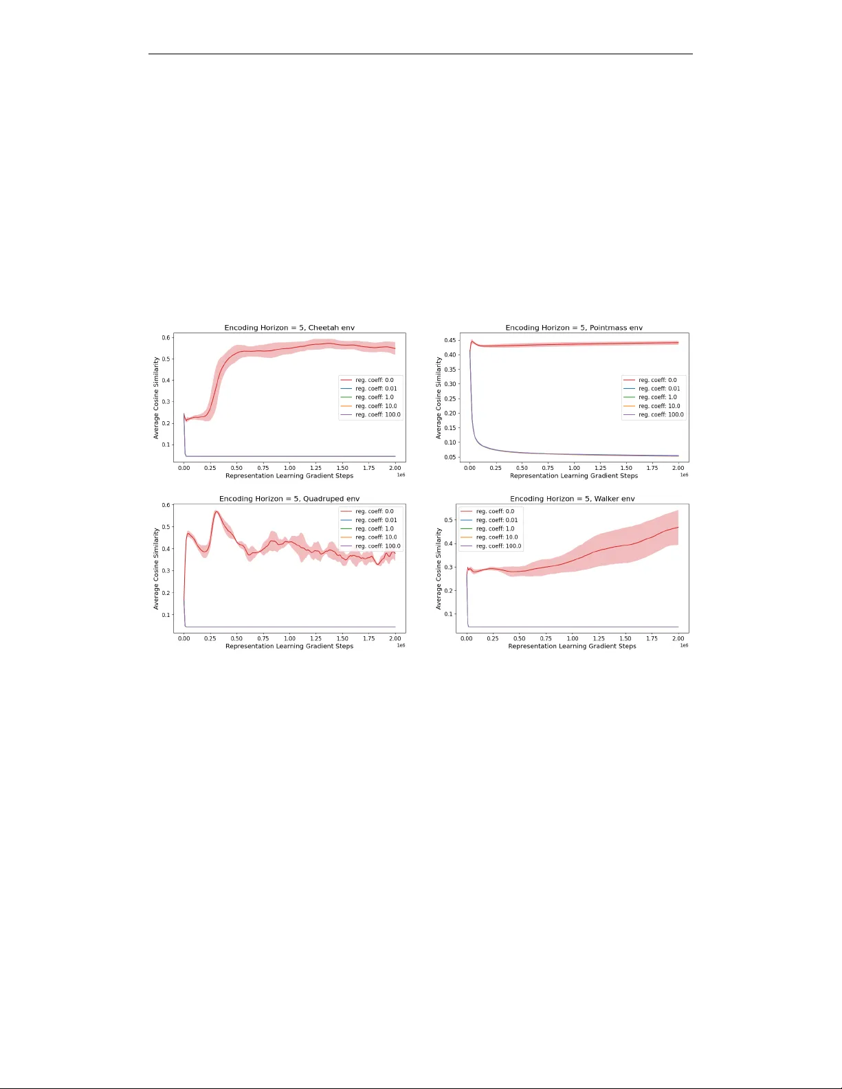
Published as a conference paper at ICLR 2026 R E G U L A R I Z E D L A T E N T D Y N A M I C S P R E D I C T I O N I S A S T R O N G B A S E L I N E F O R B E H A V I O R A L F O U N D A T I O N M O D E L S Pranaya Jajoo 1,2 ∗ Harshit Sikchi 4,† Siddhant Agarwal 4,† Amy Zhang 4 Scott Niekum 5 Martha White 1,2,3 1 Department of Computing Science, Univ ersity of Alberta, Canada 2 Alberta Machine Intelligence Institute (Amii) 3 Canada CIF AR AI Chair 4 The Univ ersity of T exas at Austin 5 Univ ersity of Massachusetts Amherst † Equal contribution A B S T R A C T Behavioral Foundation Models (BFMs) produce agents with the capability to adapt to any unkno wn re ward or task. These methods, ho wever , are only able to produce near-optimal policies for the re ward functions that are in the span of some pre-existing state features , making the choice of state features crucial to the expressivity of the BFM. As a result, BFMs are trained using a variety of complex objectiv es and require sufﬁcient dataset coverage, to train task useful spanning features. In this work, we examine the question: are these complex representation learning objectiv es necessary for zero-shot RL? Speciﬁcally , we revisit the objective of self-supervised next-state prediction in latent space for state feature learning, but observe that such an objecti ve alone is prone to increasing state-feature similarity , and subsequently reducing span. W e propose an approach, Regularized Latent Dynamics Prediction ( RLDP ), that adds a simple orthogonality regularization to maintain feature div ersity and can match or surpass state-of-the- art complex representation learning methods for zero-shot RL. Furthermore, we empirically show that prior approaches perform poorly in low-co verage scenarios where RLDP still succeeds. 1 I N T RO D U C T I O N Zero-shot reinforcement learning (RL) (T ouati et al., 2022) is a problem setting where we learn an agent that can solve any task in the en vironment without any additional training or planning, after an initial pretraining phase. Zero-shot RL has signiﬁcant practical potential in de veloping generalist agents with wide applicability . F or instance, robotics applications, like robotic manipulation or drone navigation, often require agents to solve a wide v ariety of unknown tasks. A general-purpose household robot needs to possess the capability to ﬂe xibly adapt to v arious household chores without explicit training for each ne w task. Behavioral Foundation Models (BFMs) have been shown to be promising for zero-shot RL (T ouati et al., 2022; Agarwal et al., 2024). BFMs are trained on a dataset of reward-free interactions, with the aim to pro vide a near -optimal policy for a wide class of rew ard functions without additional learning or training during test-time. BFMs are trained by a) learning a state representation φ : s → R d , and b) learning a polic y π conditioned on a latent vector z ∈ R d , where the z can be seen as a task embedding for reward r ( s ) = φ ( s ) ⊤ z . In this way , the BFM consists of a space of policies, where different policies can be extracted by querying the learned policy using different z . At test time, giv en any rew ard function r test ( s ) , the near-optimal polic y π z r test is obtained zero-shot by solving for z r test such that r test ( s ) ≈ φ ( s ) ⊤ z r test . This assumption on the re ward is also used for successor ∗ Correspondence to pranayajajoo@ualberta.ca 1 Published as a conference paper at ICLR 2026 features (Barreto et al. (2016)), which consist of the discounted cumulative sum of feature vectors under a policy . Successor features zero-shot produce the action-values for a new rew ard, giv en by vector z , and BFM approaches often use successor features to learn the policies. The performance of the BFM relies heavily on the state representation, which is both used to extract z for the rew ard and for the policy . State-of-the-art methods T ouati & Ollivier (2021); Agarwal et al. (2024); Park et al. (2024) usually learn state representations that retain information to represent successor measur es under a wide class of policies. A successor measure captures the (discounted) state visitation of a policy , giv en any starting state. They are the generalization of successor representations Dayan (1993) to continuous states, and have a simple linear relationship to successor features T ouati & Ollivier (2021). They can therefore be used to both encourage learning a generalizable state representation as well as simultaneously learning the successor features for the BFM. Successor measures are usually learned for an explicitly deﬁned class of policies (Agarwal et al., 2024) or implicitly by ﬁrst deﬁning a class of reward functions (T ouati et al., 2022; Park et al., 2024) and considering optimal policies for those rew ard functions as the set of policies. The main intuition behind predicting successor measures as a target for state representation learning is that representations suf ﬁcient to explain future state-visitation for a wide range of policies capture features that are relev ant for sequential decision making under various re ward functions. Unfortunately , learning state representations by estimating successor measures requires iterati vely applying Bellman ev aluation backups or Bellman optimality backups, both of which are known to result in a variety of learning difﬁculties. They can suffer from various forms of bias Thrun & Schwartz (2014); Fujimoto et al. (2018); Lu et al. (2018); Fu et al. (2019) and can suf fer from feature collapse due to the instability inherent in bootstrapping in the function approximation regime (Kumar et al., 2021). Using Bellman backups to learn a representation requires choosing a class of policies or a class of reward functions a priori. Further , because the state representation is trained from a batch of ofﬂine data, unless chosen carefully , the policies may select out-of- distribution actions, leading to incorrect generalization and de generate representations. A simple alternativ e that sidesteps these issues is to use latent dynamics learning: predicting future latent states giv en the current state and the sequence of actions. Learning the state representation by predicting the latent dynamics has the beneﬁt of being independent of the polic y and thus av oids using Bellman backups and these out-of-distribution issues. This work in vestigates the following question: Does latent next-state pr ediction pr oduce state featur es that enable performant zer o-shot RL? Our inv estigation is inspired by the work of Fujimoto et al. (2025), which showed that using dynamics prediction losses as auxiliary losses boosted performance of a single-task RL agent. Unlike the single task RL setting examined by Fujimoto et al. (2025), we ﬁnd that in its naiv e form, this objectiv e leads to a mild form of feature collapse where the representation of different states increase in similarity ov er training. This collapse results in poor zero-shot RL performance when ev aluated on a number of downstream tasks. W ith a simple orthogonality regularization to prev ent collapse, we sho w that the representations learned are competitiv e and present a scalable alternati ve to representations learned via complex successor measure estimation methods for zero-shot RL. In summary , the contributions of this paper are as follows. 1. W e propose regularized latent- dynamics prediction ( RLDP ) as a simple alternativ e to learn state features for zero-shot RL. W e identify as well as mitigate feature collapse plaguing latent dynamics prediction. 2. W e show that our method remains competitiv e through an extensiv e empirical ev aluation of representations for task generalization across a variety of domains, in online and ofﬂine RL settings, including in humanoid with a large state-action space. 3. W e show that the RLDP objecti ve can learn performant policies in low-co verage settings where other methods fail. 2 R E L A T E D W O R K Unsupervised RL encompasses the class of algorithms that enable learning general-purpose skills and representations without relying on reward signal in the data. W orks that have focused on intent or skill discovery hav e used diversity-dri ven objectiv es (Eysenbach et al., 2018; Achiam et al., 2018), maximizing mutual information (W arde-Farle y et al. (2018), Eysenbach et al. (2018), 2 Published as a conference paper at ICLR 2026 Achiam et al. (2018), Eysenbach et al. (2021)) or minimizing the W asserstein distance (Park et al. (2023)) between latents and the induced state-visitation distribution. These discovered skills can be used to compose optimal policies for sev eral rewards. Our work, on the other hand, focuses on learning representations capable of producing optimal value functions for any arbitrary function rew ard speciﬁcation. There are also a variety of pre-training approaches for representations that can be ﬁne-tuned for downstream control. Recent pre-training approaches (e.g., Ma et al. (2022); Nair et al. (2022)) borrow self-supervised techniques such as temporal contrastiv e objectiv es to extract embeddings from large-scale datasets (Grauman et al. (2021)). HILP (Park et al. (2024)) goes beyond standard masked autoencoding approaches by using Hilbert-space representations to preserve temporal dynamics. Auxiliary objectiv es in volve complementary predictiv e tasks to get richer semantic or temporal structures (Agarwal et al., 2021; Schwarzer et al., 2020). Although representations from auxiliary objectives can accelerate policy learning, a new policy still needs to be learned from scratch for each new re ward function. Behavioral Foundation Models are obtained by training an RL agent in an unsupervised manner using task-agnostic rew ard-free ofﬂine transitions. Forward-Backw ard representations (T ouati & Ollivier (2021)) and PSM (Ag arwal et al. (2024)) provide one such frame work for training BFMs by learning representations that capture a set of successor measures, on which sev eral successi ve works are based. Fast Imitation with BFMs (Pirotta et al. (2023)) demonstrates the ability of successor- measure–based BFMs to imitate ne w behaviors from just a fe w demonstrations, while Sikchi et al. (2025) builds upon this by ﬁne-tuning the BFM’ s latent embedding space, yielding 10-40% improv ement over their zero-shot performance. Recent progress in imitation learning has led to the dev elopment of BFMs tailored for humanoid control tasks (Peng et al. (2022), W on et al. (2022), Luo et al. (2023), T irinzoni et al. (2025)) which can produce div erse behaviors trained using human demonstration data. Our work differs from these in that it provides a new , simpler state-representation learning objectiv e for training BFMs. 3 P R E L I M I N A R I E S W e consider a reward-free Markov Decision Process (MDP) (Puterman, 2014) which is deﬁned as a tuple M = ( S , A , P, d 0 , γ ) , where S and A respectiv ely denote the state and action spaces, P denotes the transition dynamics with P ( s ′ | s, a ) indicating the probability of transitioning from s to s ′ by taking action a , d 0 denotes the initial state distribution and γ ∈ (0 , 1) speciﬁes the discount factor . A policy π is a function π : S → ∆( A ) mapping a state s to probabilities of action in A . W e denote by Pr ( · | s, a, π ) and E [ · | s, a, π ] the probability and expectation operators under state- action sequences ( s t , a t ) t ≥ 0 starting at ( s, a ) and follo wing policy π with s t ∼ P ( · | s t − 1 , a t − 1 ) and a t ∼ π ( · | s t ) . Given an y reward function r : S → R , the Q-function of π for r is Q π r ( s, a ) := P t ≥ 0 γ t E [ r ( s t +1 ) | s, a, π ] . A Behavioral F oundation Model (BFM) using Successor Featur es is a tuple ( φ, ψ , π z ) for state features, φ : S → Z , successor features deﬁned as ψ ( s, a, π ) = E π [ P t γ t φ ( s t ) | s, a ] and the task- conditioned learned policy π z that inputs any task embedding z that corresponds to a re ward function r z = φ ⊤ z . T o deﬁne this policy π z , we use action-v alues produced by the successor features ψ . The action-value function for re ward r z and a ﬁxed polic y π can be written as Q π z ( s, a ) = E π h X t γ t φ ( s t ) ⊤ z | s, a i = E π h X t γ t φ ( s t ) ⊤ | s, a i z = ψ ( s, a, π ) ⊤ z The polic y π z is the optimal policy for rew ard r z , obtained by iterativ ely greedifying o ver Q π z ( s, a ) . Using the successor feature notation, we can iterativ ely update π z for all states until it satisﬁes the following ﬁx ed-point equation π z ( ·| s ) = arg max a ψ ( s, a, π z ) ⊤ z for all s . (1) W e ov erload notation and write ψ ( s, a, z ) to mean ψ ( s, a, π z ) , because later we will directly input z into a network to learn these successor features for a near-optimal polic y for r z . The BFM can be used for any new reward function as long as we can obtain the z corresponding to that reward. This is straightforward to do if we are giv en a dataset ρ , as the corresponding z 3 Published as a conference paper at ICLR 2026 can be extracted by solving the linear regression problem, min z E ρ [( φ ⊤ z − r ) 2 ] = ( φ ⊤ φ ) − 1 φ ⊤ r . Naturally , BFMs depend heavily on the choice of the state representation φ ; ho w to learn an ef fectiv e φ is the subject of this work. Learning the successor features can be done using successor measures, instead of directly estimating the discounted sum of features φ . The successor measur e (Dayan, 1993; Blier et al., 2021) of state-action ( s, a ) under a policy π is the (discounted) distribution over future states obtained by taking action a in state s and follo wing policy π thereafter: M π ( s, a, X ) := X t ≥ 0 γ t Pr ( s t +1 ∈ X | s, a, π ) ∀ X ⊂ S . (2) The action-value can be represented as, Q π ( s, a ) = P s + M π ( s, a, s + ) r ( s + ) . This simple linear relationship between action-value functions and successor measures is similar to that of successor features and has been e xploited by recent w orks (T ouati & Olli vier, 2021; Agarwal et al., 2024; Park et al., 2024) to train BFMs. It has been shown by T ouati & Ollivier (2021) that parameterizing the successor measures as M π z ( s, a, s + ) = ψ π ( s, a, z ) ⊤ ϕ ( s + ) yields ψ ( s, a, z ) as successor features for the state feature φ ( s ) = ( ϕϕ ⊤ ) − 1 ϕ ( s ) (Theorem 12 of T ouati & Ollivier (2021)). Since, the closed form solution for z for any rew ard function r was ( φφ ⊤ ) − 1 φr , using the parameterization of M π implies z = ϕ ⊤ r . T o train the BFM , we alternate between a successor measure learning phase to get and a policy improv ement phase. The successor measure learning phase learns to model densities M π z ( s, a, s + ) using the contrastiv e objectiv e (Blier et al., 2021): Successor -measure estimation: L S M ( M π z ) = − E s,a,s ′ ∼ ρ [ M π z ( s, a, s ′ )] + 1 2 E s,a,s ′ ∼ ρ,s + ∼ ρ [( M π z ( s, a, s + ) − γ ¯ M π z ( s ′ , π z ( s ′ ) , s + )) 2 ] . (3) This objectiv e can be used assuming a ﬁxed state representation ϕ , only training the successor features ψ (as we will do for our approach), or allows for both ϕ and ψ to be jointly optimized, as was done in the Forward-Backw ard (FB) algorithm (T ouati & Ollivier, 2021), PSM (Agarwal et al., 2024) and HILP (Park et al., 2024). The policy improvement step greedily optimizes the action-value function giv en by this successor measure π z ( s ) = arg max a Q π z ( s, a ) = arg max a X s + M π z ( s, a, s + ) · r ( s + ) = arg max a X s + [ ψ ( s, a, z ) ⊤ ( ϕ ( s + ) · r ( s + ))] = arg max a ψ ( s, a, z ) ⊤ X s + ϕ ( s + ) · r ( s + ) = arg max a ψ ( s, a, z ) ⊤ z (4) In practice, we cannot directly set the policy to this argmax. Instead, we optimize the following loss. Policy Impr ovement: L P ( π z ) = − E a ∼ π z ( s ) [ ψ ( s, a, z ) ⊤ z ] (5) Appendix A.2 provides a further overvie w of approaches to train BFMs. In this work, we le verage this machinery for BFMs and focus on a new approach to estimate the state representations ϕ . 4 M E T H O D This method can be broadly divided into two parts: representation learning and zero-shot RL using successor features. The state representation encoder is trained using latent dynamics prediction with div ersity re gularization. W e will sho w that these representations lead to a reduction in the prediction error for successor measures for any policy . Lev eraging these robust state embeddings, we then pretrain a Behavioral Foundation Model (BFM) to predict successor measures, enabling zero-shot inference of near-optimal policies for unseen rew ard functions. W e refer to this method as RLDP ( R egularized L atent D ynamics P rediction based Beha vioral Foundation Policies). 4 Published as a conference paper at ICLR 2026 4 . 1 L E A R N I N G R E P R E S E N T A T I O N S W I T H R E G U L A R I Z E D L A T E N T D Y N A M I C S P R E D I C T I O N Zero-shot RL based on successor features relies on learning a state representation denoted by ϕ ( s ) . This state representation will deﬁne the span of re ward functions that the zero-shot RL method is guaranteed to output optimal policies for . The primary representation learning objectiv e is unrolled latent dynamics prediction. W e learn a state representation encoder ϕ : S → R d , ( Z = R d ) and a latent state-action representation encoder g : R d × A → R d such that latent dynamics can be expressed as ϕ ( s ′ ) = g ( ϕ ( s ) , a ) ⊤ w with some learned weights w , informing our loss function for representation learning. A sub-sequence of horizon H is sampled from the of ﬂine interaction dataset ρ giv en by τ i = { s i 0 , a i 0 , s i 1 , a i 1 , ..., s i H − 1 , a i H − 1 , s i H } . A sequence of future latent states h i 1: H are obtained by encoding the initial state h i 0 = ϕ ( s i 0 ) and unrolling using the deﬁned dynamics model h i t +1 = g ( h i t , a t ) ⊤ w . Then the objectiv e is to predict the encoded future latent states: L d ( ϕ, g , w ) = E τ i ∼ d O        H X t =1 h i t − ¯ ϕ ( s i t )      2   , (6) where τ i = { s i 0 , a i 0 , s i 1 , a i 1 , ..., s i H − 1 , a i H − 1 , s i H } , h i 0 = ϕ ( s i 0 ) , and ¯ ϕ is the slowly moving encoder target, which is periodically set to ϕ . Figure 1: A verage Cosine similarity between state- representations sampled uniformly from the training dataset. Feature similarity increases over the course of training; once adding our orthogonality regularizer (with λ = 1 ), we obtain more diverse representations. Shaded region sho ws standard deviation o ver 4 seeds. Latent dynamics models hav e been shown to signiﬁcantly improve sample efﬁciency for single task RL when models are used for planning (Hansen et al., 2022), learning (Hafner et al., 2019), or as representations (Fujimoto et al., 2025) for model-free RL, but their suitability as general-purpose representations for multi-task and zero-shot RL remains understudied. Most successful methods (T ouati & Olli vier, 2021; Ag arwal et al., 2024) for zero-shot RL train representations to predict successor measures. Howe ver , directly estimating successor measures requires learning future state-occupancies under a predeﬁned set of policies. This poses a problem in the low-co verage setting as Bellman backups with policies that choose out of distribution action will result in incorrect predictions and neg ativ ely af fect representation learning. In contrast, latent dynamics prediction is a policy-independent representation learning objecti ve. Howe ver , solely learning with the latent dynamics objecti ve can lead to conv ergence to a collapsed solution. This is unsurprising as trivial solutions of predicting a constant zero vector achieves a perfect loss in equation 6. T o combat this, prior works (Grill et al., 2020) have proposed the use of a semi-gradient update where a stop-gradient is used for target h t +1 in equation 6 along with a slowly updating target. Howe ver , we ﬁnd these techniques insuf ﬁcient to maintain representation div ersity . W e in vestigate this by computing the cosine similarity of state representations as a function of gradient steps trained via minimizing equation 6 on an of ﬂine dataset collected by an e xploration algorithm RND (Burda et al., 2018). Figure 1 shows that while the solutions do not collapse, there is an increase in feature similarity over the course of learning, which we refer to as a mild form of collapse. As the space of reward functions is spanned by state features, such an increase in feature similarity directly reduce the class of reward functions for which we can learn optimal policies and negati vely impact task generalization. Mitigating collapse in latent dynamics prediction: In order to prevent the mild form of feature collapse discussed earlier , we propose to add an auxiliary regularization objective that encourages div ersity . Orthogonal regularization has been also studied in self-supervised learning (He et al., 2024; Bansal et al., 2018) as a way to mitigate collapse. W e project all state representations ϕ as well as predicted latent ne xt-state g ( ϕ ( s ) , a ) ⊤ w in a hypersphere: S d − 1 = { x ∈ R d : ∥ x ∥ 2 = √ d } and regularize by minimizing cosine similarity between any two states. W e 5 Published as a conference paper at ICLR 2026 ablate the choice of hyperspherical normalization on g in Appendix A.4.2 and observe it to giv e consistent improvements. W e note that a similar regularization was applied to state features in the implementation for Forward-Backward representations (T ouati et al., 2022) to encourage solution identiﬁability and uniqueness. In the case of latent dynamics prediction this step becomes crucial to mitigate the increase in representation similarity . Figure 2: RLDP combines latent next state prediction + regularization for div ersity (an orthogonality regularizer) to learn representations for BFMs. The orthogonal regularization loss takes the following form: L r ( ϕ ) = E s,s ′ ∼ ρ [ ϕ ( s ) ⊤ ϕ ( s ′ )] (7) where ϕ ∈ S d − 1 . Our ﬁnal loss is a weighted combination of dynamics prediction combined with orthogonal div ersity regularization L RLD P ( ϕ, g , w ) = L d ( ϕ, g , w ) + λ L r ( ϕ ) (8) where λ controls the regularization strength. W e visualize this loss in ﬁgure 2, where the encoder is gi ven by ϕ , the dynamics by g and w and the div ersity across encoded states is encouraged with L r . W e ﬁnd that adding this regularization prev ents collapse, shown in ﬁgure 1, ev en with a relativ ely small regularization coefﬁcient λ = 0 . 01 . W e e valuate the impact of orthogonality regularization further with other coefﬁcients λ in Appendix section A.4.2. RLDP leads to repr esentations capable of predicting successor measures: The representation learning objecti ve is simply latent dynamics prediction with an orthogonal regularization. Through this objective, we are enforcing the representations to be good for predicting successor measures, which forms the basis of the BFMs that will be constructed using these. While prior work (Agarwal et al., 2025) already indicate that these representations are suitable for predicting successor measures, we further formalize this intuition. Let’ s begin by looking at the latent space abstract MDP ¯ M deﬁned using the state representation ϕ . Deﬁnition 4.1. Let MDP ¯ M corr esponding to the state abstraction ϕ : S → Z be deﬁned as < ϕ ( s ) , A , P ( ·| ϕ ( s ) , a ) , γ , r > . Apart from facilitating the construction of BFMs and zero-shot RL, one of the utilities of the state-representations is to compress the state space to a smaller space. MDP ¯ M represents this compression. W e will assume that ¯ M is Lipschitz. Formally , Assumption 4.2. ¯ M is ( K R , K P ) − Lipschitz . (Gelada et al., 2019) W e now have all the components to show in the Lemma 4.3 that minimizing L RLD P will lead to a reduction in the prediction error of successor measure for any K V -Lipschitz valued polic y . Lemma 4.3. Given MDP ¯ M , let π be any K V -Lipschitz valued policy , M π be the successor measur e for π and ¯ M π be the corr esponding successor measur e on ¯ M , L RLD P ( ϕ, g , w ) upper bounds the pr ediction err or in successor measur e, E s,a ∼ d π ,s + ∼ ρ [ | M π ( s, a, s + ) − ¯ M π ( ϕ ( s ) , a, ϕ ( s + )) | ] ≤ L RLD P ( ϕ, g , w ) 1 − γ (9) 4 . 2 Z E R O - S H OT R L W I T H RLDP R E P R E S E N T A T I O N S The ﬁrst step to use RLDP is to train the representations from a batch of re ward-free of ﬂine en vironment transitions. The RLDP representation loss giv en in equation 8 does not rely on rew ard, because it only uses the latent dynamics prediction loss and the orthogonality regularizer . 6 Published as a conference paper at ICLR 2026 It is straightforward to optimize this loss on the batch of ofﬂine data, to obtain a learned state representation ϕ . Ke y choices to be made include the regularization coefﬁcient λ , the length of the rollout H for the latent dynamics prediction loss and the update frequency for encoder target ¯ ϕ . The next step is to train the BFM, by alternating successor measure estimation and policy improv ement. The RLDP representations are kept frozen in the successor measure parameterization M π z ( s, a, s + ) = ψ π ( s, a, z ) ⊤ ϕ ( s + ) and ψ ( s, a, z ) and π z are trained using losses 10 and 5 respectiv ely . L z srl ( ψ ) = − E s,a,s ′ ∼ ρ [ ψ ( s, a, z ) ϕ ( s ′ )] + 1 2 E s,a,s ′ ∼ ρ,s + ∼ ρ [( ψ ( s, a, z ) ϕ ( s + ) − γ ¯ ψ ( s ′ , π z ( s ′ ) , z ) ϕ ( s + )) 2 ] (10) Follo wing prior work, in our experiments we consider variations of the policy improvement step (Eq 5) where we use an expert regularization in the policy update (Tirinzoni et al., 2025) to guide exploration during online RL for high-dimensional state-action spaces or use a behavior cloning regularization (Fujimoto & Gu, 2021) when learning ofﬂine for lo w-coverage datasets. These modiﬁcations are discussed in detail in the next section. W e provide the full representation and policy learning pipeline for RLDP in Appendix section A.6. 5 E X P E R I M E N T S The goal of our experiments is to perform an extensiv e empirical study of the suitability of state representations learned by a regularized latent next-state prediction objectiv e when compared to other methods that employ more complex strategies. In particular, we aim to answer the following questions: (a) Keeping all other learning factors similar , ho w does our method compare to baselines in enabling generalization to unseen reward functions? W e compare the representations learned by training multi-task policies with zero-shot RL both in the ofﬂine setting and the online setting. (b) By avoiding querying actions out of distribution does RLDP provide a robust choice for learning representations in low cov erage datasets? (c) What design decisions are crucial to the success of our method? W e perform extensiv e ablation studies to understand our design choices. For all datasets, we pretrain a BFM using the successor feature approach outlined in our method section 4. Each algorithm is gi ven the same budget of gradient steps during pretraining, controlling the state representation dimension, and the ﬁnal performance is obtained by taking the pre-trained model at the end and querying it for different task-re wards for 50 episodes. 5 . 1 B E N C H M A R K I N G Z E R O - S H OT R L F O R C O N T I N U O U S C O N T RO L T ask Random Features FB PSM RLDP W alker Stand 392.40 ± 58.03 918.29 ± 28.83 899.54 ± 30.73 890.40 ± 27.33 Run 75.39 ± 20.97 381.31 ± 17.32 450.57 ± 28.95 334.26 ± 49.69 W alk 193.84 ± 112.98 779.29 ± 63.60 875.61 ± 33.44 779.77 ± 137.16 Flip 132.02 ± 67.85 977.08 ± 2.76 621.36 ± 75.62 492.94 ± 22.79 Cheetah Run 31.82 ± 36.88 129.39 ± 37.63 181.85 ± 54.17 157.12 ± 29.92 Run Backward 60.08 ± 12.82 142.41 ± 36.77 158.64 ± 18.56 170.52 ± 15.30 W alk 147.52 ± 155.66 604.54 ± 80.51 576.98 ± 209.45 592.92 ± 104.66 W alk Backward 272.77 ± 42.40 630.40 ± 144.23 817.92 ± 98.86 821.51 ± 50.62 Quadruped Stand 240.01 ± 66.06 732.59 ± 101.33 708.03 ± 34.99 794.94 ± 43.25 Run 114.19 ± 30.22 425.15 ± 52.02 404.32 ± 23.26 457.41 ± 74.70 W alk 137.65 ± 47.57 492.91 ± 17.55 523.94 ± 52.13 465.40 ± 185.29 Jump 190.62 ± 46.63 567.27 ± 48.90 549.57 ± 15.86 733.32 ± 55.30 Pointmass T op Left 258.59 ± 183.56 943.85 ± 17.31 924.20 ± 10.64 890.41 ± 60.79 T op Right 216.30 ± 189.05 550.84 ± 282.41 666.00 ± 133.15 795.47 ± 21.10 Bottom Left 193.32 ± 90.37 672.28 ± 153.06 800.93 ± 15.62 805.17 ± 20.44 Bottom Right 64.08 ± 72.21 272.97 ± 274.99 123.44 ± 138.82 193.38 ± 167.63 T able 1: Comparison (ov er 4 seeds) of zero-shot RL performance between using an untrained initialized encoder , FB, PSM, and RLDP with representation size d = 512 . Bold indicates the best mean and any method whose mean plus one standard deviation o verlaps with the best mean. Baselines: W e broadly compare RLDP against commonly used state- of-the-art baselines for zero-shot RL such as: FB, PSM, and HILP . These baselines represent a set of diverse and strong approaches in the area of zero-shot RL. 5 . 1 . 1 O FFL I N E Z E RO - S H OT R L Setup: W e consider continuous control tasks from DeepMind control suite (T assa et al., 2018) – Pointmass, Cheetah, W alker , Quadruped under a similar setup considered 7 Published as a conference paper at ICLR 2026 by prior works in zero-shot RL. W e use datasets from the ExoRL suite (Y arats et al. (2022)) that are obtained by an exploratory algorithm RND (Burda et al. (2018)). Random features use representations from a randomly initialized NN encoder . Evaluation: T o ev aluate the different zero-shot RL methods we take the pretrained policies and query them on a variety of tasks. For each en vironment, we consider 4 tasks similar to prior works (T ouati et al., 2022; Park et al., 2024; Agarwal et al., 2024). W e conduct our experiments across two axes: a) T able 1 pretrains all the BFMs on same number of representation dimensions (512) and gradient steps. For RLDP , we use an encoding horizon of 5. W e train representations for 2 million steps and train policy for additional 3 million steps. b) T able 6 in the Appendix compares against representation dimension for ϕ found to be best for prior methods and RLDP with the same number of gradient updates for pretraining each BFM. Results: Overall, using learned representations (FB, PSM, RLDP ) outperforms random features, conﬁrming that representation learning is crucial for zero-shot RL. Among learned methods, PSM and RLDP generally achieve the strongest performance. Furthermore, training FB and PSM baselines is sensiti ve to hyperparameters and we rely on author’ s implementation to tune hyperparameters. 5 . 1 . 2 O N L I N E Z E R O - S H OT R L Previous section validated that RLDP representations lead to competitive zero-shot RL when the learning policies use ofﬂine interaction data. W e explore if the learned representation enable competitiv e multi-task learning when agent is allowed interaction with the en vironment. Figure 3: Pair -wise comparison of RLDP against prior ofﬂine representation learning methods using per-task oracle normalized performance differences ( ∆ = RLDP – Baseline) in SMPL Humanoid environment. The gray diamond represents the IQM (Interquartile Mean). Setup: W e consider the SMPL (Loper et al. (2015)) Humanoid en vironment that aims to mimic real human embodiment and provides a complex learning challenge with a 358 dimensional observation space and a 69 dimensional action space. Due to the exploratory challenge of the en vironment, T irinzoni et al. (2025) presented a ne w approach, Conditional Policy Regularization (CPR), to guide RL learning regularized with expert real-human trajectories. CPR trains successor measures in a similar way as equation 3 but adds a regularization objectiv e to policy encouraging it to jointly maximize Q -function while staying close to expert. This allows for better exploration and more realistic motions. Further implementation details can be found in appendix sections A.3.2, A.5.2. Evaluation: Our representation learning phase is ofﬂine and we use the metamoti vo 5M transition dataset 1 collected from replay buf fer of an online RL agent to learn state-representations and then use the CPR approach to train zero-shot policies. W e train representations for 2 million gradient steps and policy for 20 million environment steps. The ofﬂine phase of representation learning helps us remov e the exploration confounder and test the quality of representations obtained by different approaches. The e valuation is performed on the full suite of 45 tasks pro vided by Tirinzoni et al. (2025). For each task, we present the normalized scores with respect to fully-online trained representations and policy in table 8 and we present the aggregates results across tasks in ﬁgure 3 ov er 4 seeds. Results: Figure 3 summarizes the results of RLDP representations with respect to baseline methods across all 45 tasks. Positive values indicate tasks where RLDP achieves higher normalized returns. These results suggest that ov erall RLDP fares competiti vely to the baselines. Complete results for this e valuation are provided in table 8. Further analysis shows that the performance is task dependent - on some tasks (such as raisearms and lieonground), RLDP outperforms the baselines, e ven beating 1 https://huggingface.co/facebook/metamoti vo-M-1 8 Published as a conference paper at ICLR 2026 the oracle performance for some tasks (shown in table 8). In others (like crawl or rotate tasks), all methods perform subpar to oracle. 5 . 2 L E A R N I N G R E P R E S E N T A T I O N S W I T H L OW C OV E R A G E D AT A S E T S RLDP learns a policy-independent representation through latent dynamics prediction. Prior approaches assume a class of policies to learn representations predictive of successor measures, and this strategy can lead to poor out-of-distribution generalization when actions proposed by the policy are not co vered by the dataset. Setup. T o ev aluate this hypothesis concretely , we consider the D4RL benchmark of OpenAI Gym MuJoCo tasks (Fu et al. (2020), T odorov et al. (2012), Brockman et al. (2016)). This dataset has been widely used to examine the effects of value estimation error from out-of-distribution actions due to low cov erage, which man y of ﬂine RL algorithms struggle with (Kostrik ov et al. (2021); Fujimoto & Gu (2021); Kumar et al. (2020); W u et al. (2019); Sikchi et al. (2023)). W e consider halfcheetah, hopper , and walker2d domains, and medium and medium-e xpert datasets. Figure 4: Pair -wise comparison of RLDP against baseline representation learning methods in low-co verage D4RL dataset. Each point represents ∆ = R RLDP − R baseline for a single { task , seed } pair . The gray diamond represents the IQM (Interquartile Mean). Evaluation: T o ev aluate the different zero-shot RL methods, we ﬁrst pretrain the representation learning methods on these datasets for 1 million gradient steps. W e use a modiﬁed zero-shot policy learning approach that alternates between equation 3 and equation 5 that is additionally augmented policy improv ement loss with a behavioral regularization inspired by Fujimoto & Gu (2021). This regularization allow the RL approach to learn without overestimation bias and enabling us to establish a fair comparison among representations learned by different approaches. W e use the corresponding reward function provided by each dataset to do rew ard inference and e valuate the zero-shot policy . Further details are provided in Appendix sections A.3.3 and A.5.3. Results: Figure 4 shows one-to-one comparison of normalized returns of RLDP against baseline methods using paired per-seed performance dif ferences across 6 low-co verage D4RL tasks over 10 seeds. RLDP outperforms all baseline methods in 5 out of 6 tasks. The overall mass of the violin lies abov e zero and IQM is positiv e, indicating that RLDP achieves higher normalized returns compared to the baseline. Overall, the results suggest that RLDP is a reliable choice for feature learning in low coverage datasets while providing a simpler alternative to otherwise complex representation learning approaches. Per task normalized scores and statistical signiﬁcance testing is reported in the Appendix section A.9 and table 9. W e further bisect the indi vidual and combined impact of using Bellman backups (similar to FB which may query out-of-distribution actions), latent next-state prediction, and orthogonality regularization for representation learning in section A.11 and ﬁnd explicit Bellman backups to hurt performance of learned policy . 5 . 3 W H AT M A T T E R S F O R S U P E RV I S I N G R E P R E S E N TA T I O N S S U I T A B L E F O R C O N T RO L ? In section 4, we introduced RLDP method of representation learning with the loss used (equation 8) and the encoder training process. In this section, we aim to ablate components of this loss and the architecture of the encoder . Orthogonality regularization: K eeping the encoding horizon constant ( H = 5) , we change the orthogonality regularization coefﬁcient. The results, presented in Figure 5, show that for zero regularization ( λ = 0 ), the average return decreases compared to λ > 0 . This shows that 9 Published as a conference paper at ICLR 2026 div ersity regularization is critical to the representation loss. For ﬁxed encoding horizon, we see that orthogonality regularizer λ = 1 performs best. T o further understand the role of the orthogonality regularizer in representation learning and how it helps prev ent feature collapse, we refer to section 4 and section A.4.2, where we show that the learned representations increase in cosine similarity without regularization. Figure 5: Evaluating the impact of Orthogonality Regularization: W e ran one-sided Mann–Whitney U tests on the per-seed returns ov er 4 seeds to compare different values of the orthogonality regularization, and we observe that adding small orthogonality regularization coefﬁcient λ = 0 . 01 gi ves a statistically signiﬁcant improv ement over coef ﬁcient λ = 0 . 0 . Encoder architectur e: In section 4.1, we introduce encoder training, where we project the latent next state representation g ( ϕ ( s ) , a ) .w to a hypersphere. Here, we ablate the importance of this projection. The results are presented in table 2. W e observe that RLDP consistently outperforms its v ariant without spherical normalization on most tasks. The standard de viation is also higher for most results on the variant without hypersphere projection. This indicates that spherical normalization is an important design choice for stabilization and improving performance. Results for all en vironments are reported in table 5. W e provide additional discussion of the complete encoder architecture in section A.4, where we further ablate the encoder architecture. 6 C O N C L U S I O N T ask RLDP RLDP w/o SN Quadruped Stand 794.94 ± 43.25 661.73 ± 95.75 Run 457.41 ± 74.70 378.97 ± 148.47 W alk 465.40 ± 185.29 519.39 ± 251.11 Jump 733.32 ± 55.30 495.98 ± 133.81 A verage(*) 612.77 ± 83.17 514.02 ± 86.94 Pointmass T op Left 890.41 ± 60.79 892.13 ± 41.74 T op Right 795.47 ± 21.10 728.72 ± 122.99 Bottom Left 805.17 ± 20.44 683.12 ± 76.22 Bottom Right 193.38 ± 167.63 22.54 ± 39.04 A verage(*) 671.11 ± 292.58 581.63 ± 341.00 T able 2: Study of encoder architecture (subset). T able shows mean ± std; RLDP signiﬁcantly outperforms RLDP w/o SN on Pointmass, Quadruped, and pooled. SN: Spherical Normalization on g . This paper introduces RLDP , a representation learning objective for ef fectiv e task generalization enabling performant behavioral foundation models. Our objecti ve takes the simple form of regularized latent- dynamics prediction, an objectiv e that does not require any reconstruction, making it able to handle high-dimensional observation space and does not require explicit Bellman backups, making it more amenable to optimization. W e identify that simply using latent-dynamics prediction leads to a mild form of feature collapse where the state-representation similarity increases over time. T o combat this issue, we propose using orthogonal regularization as a w ay to maintain feature div ersity and prev ent collapse. Using our method enables learning generalizable, stable, and robust representations that can achieve competitiv e performance compared to prior zero-shot RL techniques without relying on reinforcement-driven signals. Importantly , we show that prior approaches struggle in low cov erage setting and RLDP works robustly across different dataset types, making it a practical unsupervised learning approach. This work, thus, pav es the way for simpler yet effecti ve approaches to learn zero-shot policies in behavioral foundation models. 10 Published as a conference paper at ICLR 2026 7 A C K N O W L E D G E M E N T S W e thank Siddarth Chandrasekar , Dikshant Shehmar , and Diego Gomez for enlightening discussions on unsupervised RL. This work has been conducted at the Reinforcement Learning and Artiﬁcial Intelligence (RLAI) lab at the Univ ersity of Alberta, the Safe, Correct, and Aligned Learning and Robotics Lab (SCALAR) at the Univ ersity of Massachusetts Amherst, and Machine Intelligence through Decision-making and Interaction (MIDI) Lab at The Uni versity of T exas at Austin. Support for this work was provided by the Canada CIF AR AI Chair Program, the Alberta Machine Intelligence Institute, and the Natural Sciences and Engineering Research Council of Canada (NSERC). HS, SA, and AZ are supported by NSF 2340651, NSF 2402650, DARP A HR00112490431, and ARO W911NF-24-1-0193. W e are also grateful for the computational resources provided by the Digital Research Alliance of Canada. R E F E R E N C E S Joshua Achiam, Harrison Edwards, Dario Amodei, and Pieter Abbeel. V ariational option discovery algorithms. arXiv preprint , 2018. Siddhant Agarwal, Aaron Courville, and Rishabh Agarwal. Behavior predictiv e representations for generalization in reinforcement learning. In Deep RL W orkshop Neural Information Processing Systems 2021 , 2021. URL https://openreview.net/forum?id=b5PJaxS6Jxg . Siddhant Agarwal, Harshit Sikchi, Peter Stone, and Amy Zhang. Proto successor measure: Representing the space of all possible solutions of reinforcement learning. arXiv preprint arXiv:2411.19418 , 2024. Siddhant Agarwal, Caleb Chuck, Harshit Sikchi, Jiaheng Hu, Max Rudolph, Scott Niekum, Peter Stone, and Amy Zhang. A uniﬁed frame work for unsupervised reinforcement learning algorithms. In W orkshop on Reinfor cement Learning Be yond Rewar ds@ Reinfor cement Learning Confer ence 2025 , 2025. Nitin Bansal, Xiaohan Chen, and Zhangyang W ang. Can we gain more from orthogonality regularizations in training deep cnns? arXiv pr eprint arXiv:1810.09102 , 2018. Andr ´ e Barreto, R ´ emi Munos, T om Schaul, and David Silver . Successor features for transfer in reinforcement learning. arXiv preprint , 2016. L ´ eonard Blier, Corentin T allec, and Y ann Ollivier . Learning successor states and goal-dependent values: A mathematical viewpoint. arXiv preprint , 2021. Greg Brockman, V icki Cheung, Ludwig Pettersson, Jonas Schneider , John Schulman, Jie T ang, and W ojciech Zaremba. Openai gym. arXiv pr eprint arXiv:1606.01540 , 2016. Y uri Burda, Harrison Edwards, Amos Storkey , and Oleg Klimov . Exploration by random network distillation. arXiv preprint , 2018. Peter Dayan. Improving generalization for temporal difference learning: The successor representation. Neural computation , 5(4):613–624, 1993. Benjamin Eysenbach, Abhishek Gupta, Julian Ibarz, and Sergey Levine. Di versity is all you need: Learning skills without a rew ard function. arXiv preprint , 2018. Benjamin Eysenbach, Ruslan Salakhutdinov , and Sergey Levine. The information geometry of unsupervised reinforcement learning. arXiv preprint , 2021. Justin Fu, A viral Kumar , Matthew Soh, and Sergey Le vine. Diagnosing bottlenecks in deep q- learning algorithms. arXiv preprint , 2019. Justin Fu, A viral Kumar , Oﬁr Nachum, George T ucker , and Sergey Le vine. D4rl: Datasets for deep data-driv en reinforcement learning. arXiv preprint , 2020. Scott Fujimoto and Shixiang Shane Gu. A minimalist approach to ofﬂine reinforcement learning. arXiv pr eprint arXiv:2106.06860 , 2021. 11 Published as a conference paper at ICLR 2026 Scott Fujimoto, David Meger , and Doina Precup. Off-policy deep reinforcement learning without exploration. corr abs/1812.02900 (2018). arXiv pr eprint arXiv:1812.02900 , 2018. Scott Fujimoto, Pierluca D’Oro, Amy Zhang, Y uandong T ian, and Michael Rabbat. T ow ards general-purpose model-free reinforcement learning. arXiv preprint , 2025. Carles Gelada, Saurabh Kumar , Jacob Buckman, Oﬁr Nachum, and Marc G Bellemare. Deepmdp: Learning continuous latent space models for representation learning. In International confer ence on machine learning , pp. 2170–2179. PMLR, 2019. K Grauman, A W estb ury , E Byrne, Z Chavis, A Furnari, R Girdhar , J Hamburger , H Jiang, M Liu, X Liu, et al. Ego4d: around the world in 3,000 hours of egocentric video. arxiv 2021. arXiv pr eprint arXiv:2110.07058 , 2021. Jean-Bastien Grill, Florian Strub, Florent Altch ´ e, Corentin T allec, Pierre H Richemond, Elena Buchatskaya, Carl Doersch, Bernardo A vila Pires, Zhaohan Daniel Guo, Mohammad Gheshlaghi Azar , et al. Bootstrap your o wn latent: A new approach to self-supervised learning. eprint arXiv: 2006.07733 , 2020. T uomas Haarnoja, Aurick Zhou, Pieter Abbeel, and Sergey Le vine. Soft actor-critic: Off- policy maximum entropy deep reinforcement learning with a stochastic actor . arXiv preprint arXiv:1801.01290 , 2018. Danijar Hafner, Timothy Lillicrap, Jimmy Ba, and Mohammad Norouzi. Dream to control: Learning behaviors by latent imagination. arXiv preprint , 2019. Nicklas Hansen, Xiaolong W ang, and Hao Su. T emporal difference learning for model predicti ve control. arXiv preprint , 2022. Junlin He, Jinxiao Du, and W ei Ma. Prev enting dimensional collapse in self-supervised learning via orthogonality regularization. arXiv pr eprint arXiv:2411.00392 , 2024. Ilya K ostrikov , Ashvin Nair , and Sergey Levine. Of ﬂine reinforcement learning with implicit q- learning. arXiv preprint , 2021. A viral K umar , Aurick Zhou, Geor ge T ucker , and Ser gey Le vine. Conservati ve q-learning for ofﬂine reinforcement learning. arXiv preprint , 2020. A viral Kumar , Rishabh Agarwal, T engyu Ma, Aaron Courville, George T ucker , and Serge y Levine. Dr3: V alue-based deep reinforcement learning requires explicit regularization. arXiv preprint arXiv:2112.04716 , 2021. Y itang Li, Zhengyi Luo, T onghe Zhang, Cunxi Dai, Anssi Kanervisto, Andrea Tirinzoni, Haoyang W eng, Kris Kitani, Mateusz Guzek, Ahmed T ouati, et al. Bfm-zero: A promptable behavioral foundation model for humanoid control using unsupervised reinforcement learning. arXiv pr eprint arXiv:2511.04131 , 2025. Matthew Loper, Naureen Mahmood, Javier Romero, Gerard Pons-Moll, and Michael J Black. Smpl: A skinned multi-person linear model. ACM T ransactions on Gr aphics , 34(6), 2015. T yler Lu, Dale Schuurmans, and Craig Boutilier . Non-delusional q-learning and value-iteration. Advances in neural information pr ocessing systems , 31, 2018. Zhengyi Luo, Jinkun Cao, Josh Merel, Alexander Winkler , Jing Huang, Kris Kitani, and W eipeng Xu. Univ ersal humanoid motion representations for physics-based control. arXiv preprint arXiv:2310.04582 , 2023. Y echeng Jason Ma, Shagun Sodhani, Dinesh Jayaraman, Osbert Bastani, V ikash Kumar , and Amy Zhang. V ip: T owards universal visual re ward and representation via value-implicit pre-training. arXiv pr eprint arXiv:2210.00030 , 2022. Suraj Nair , Aravind Rajeswaran, V ikash Kumar , Chelsea Finn, and Abhinav Gupta. R3m: A univ ersal visual representation for robot manipulation. arXiv preprint , 2022. 12 Published as a conference paper at ICLR 2026 Seohong P ark, Oleh Rybkin, and Serge y Le vine. Metra: Scalable unsupervised rl with metric-a ware abstraction. arXiv preprint , 2023. Seohong Park, T obias Kreiman, and Serge y Levine. F oundation policies with hilbert representations. arXiv pr eprint arXiv:2402.15567 , 2024. Xue Bin Peng, Y unrong Guo, Lina Halper, Sergey Levine, and Sanja Fidler . Ase: Large-scale reusable adversarial skill embeddings for physically simulated characters. A CM T ransactions On Graphics (T OG) , 41(4):1–17, 2022. Matteo Pirotta, Andrea T irinzoni, Ahmed T ouati, Alessandro Lazaric, and Y ann Ollivier . F ast imitation via behavior foundation models. In NeurIPS 2023 F oundation Models for Decision Making W orkshop , 2023. Martin L Puterman. Marko v decision pr ocesses: discrete stochastic dynamic pr ogramming . John W iley & Sons, 2014. Max Schwarzer , Ankesh Anand, Rishab Goel, R De von Hjelm, Aaron Courville, and Philip Bachman. Data-efﬁcient reinforcement learning with self-predicti ve representations. arXiv pr eprint arXiv:2007.05929 , 2020. Harshit Sikchi, Qinqing Zheng, Amy Zhang, and Scott Niekum. Dual rl: Uniﬁcation and new methods for reinforcement and imitation learning. arXiv preprint , 2023. Harshit Sikchi, Siddhant Agarwal, Pranaya Jajoo, Samyak Parajuli, Caleb Chuck, Max Rudolph, Peter Stone, Amy Zhang, and Scott Niekum. Rlzero: Direct policy inference from language without in-domain supervision. arXiv preprint , 2024. Harshit Sikchi, Andrea Tirinzoni, Ahmed T ouati, Y ingchen Xu, Anssi Kanervisto, Scott Niekum, Amy Zhang, Alessandro Lazaric, and Matteo Pirotta. Fast adaptation with beha vioral foundation models. arXiv preprint , 2025. Y uv al T assa, Y otam Doron, Alistair Muldal, T om Erez, Y azhe Li, Diego de Las Casas, David Budden, Abbas Abdolmaleki, Josh Merel, Andre w Lefrancq, et al. Deepmind control suite. arXiv pr eprint arXiv:1801.00690 , 2018. Chen T essler, Y ifeng Jiang, Erwin Coumans, Zhengyi Luo, Gal Chechik, and Xue Bin Peng. Maskedmanipulator: V ersatile whole-body control for loco-manipulation. arXiv pr eprint arXiv:2505.19086 , 2025. Sebastian Thrun and Anton Schwartz. Issues in using function approximation for reinforcement learning. In Pr oceedings of the 1993 connectionist models summer school , pp. 255–263. Psychology Press, 2014. Andrea T irinzoni, Ahmed T ouati, Jesse Farebrother , Mateusz Guzek, Anssi Kanervisto, Y ingchen Xu, Alessandro Lazaric, and Matteo Pirotta. Zero-shot whole-body humanoid control via behavioral foundation models. arXiv preprint , 2025. Emanuel T odorov , T om Erez, and Y uval T assa. Mujoco: A physics engine for model-based control. In 2012 IEEE/RSJ international conference on intelligent robots and systems , pp. 5026–5033. IEEE, 2012. Ahmed T ouati and Y ann Ollivier . Learning one representation to optimize all rewards. arXiv pr eprint arXiv:2103.07945 , 2021. Ahmed T ouati, J ´ er ´ emy Rapin, and Y ann Ollivier . Does zero-shot reinforcement learning exist? arXiv pr eprint arXiv:2209.14935 , 2022. David W arde-Farle y , T om V an de Wiele, T ejas Kulkarni, Catalin Ionescu, Stev en Hansen, and V olodymyr Mnih. Unsupervised control through non-parametric discriminative rewards. arXiv pr eprint arXiv:1811.11359 , 2018. Jungdam W on, Deepak Gopinath, and Jessica Hodgins. Physics-based character controllers using conditional vaes. ACM T ransactions on Gr aphics (TOG) , 41(4):1–12, 2022. 13 Published as a conference paper at ICLR 2026 Y ifan W u, George T ucker , and Oﬁr Nachum. The laplacian in rl: Learning representations with efﬁcient approximations. arXiv preprint , 2018. Y ifan W u, George T ucker , and Oﬁr Nachum. Behavior regularized ofﬂine reinforcement learning. arXiv pr eprint arXiv:1911.11361 , 2019. Denis Y arats, David Brandfonbrener , Hao Liu, Michael Laskin, Pieter Abbeel, Alessandro Lazaric, and Lerrel Pinto. Don’t change the algorithm, change the data: Exploratory data for ofﬂine reinforcement learning. arXiv preprint , 2022. 14 Published as a conference paper at ICLR 2026 A A P P E N D I X A . 1 P R O O F O F L E M M A 4 . 3 Lemma A.1. Given MDP ¯ M , let π be any K V -Lipschitz valued policy , M π be the successor measur e for π and ¯ M π be the corr esponding successor measur e on ¯ M , L RLD P ( ϕ, g , w ) upper bounds the pr ediction err or in successor measur e, E s,a ∼ d π ,s + ∼ ρ [ | M π ( s, a, s + ) − ¯ M π ( ϕ ( s ) , a, ϕ ( s + )) | ] ≤ L RLD P ( ϕ, g , w ) 1 − γ (9) Pr oof. Let’ s begin with E s,a ∼ d π [ | M π ( s, a, s + ) − ¯ M π ( s, a, s + )] . For a ﬁx ed s + E s,a ∼ d π [ | M π ( s, a, s + ) − ¯ M π ( s, a, s + )] ≤ E s,a ∼ d π | p ( s ′ = s + ) − p ( ϕ ( s ′ ) = ϕ ( s + )) | + γ E s,a ∼ d π | E s ′ ∼ P ( ·| s,a ) V π ( s ′ ) − E ϕ ( s ′ ) ∼ P ( ·| ϕ ( s ) ,a ) V π ( ϕ ( s ′ ) | ≤ L R + γ E s,a ∼ d π | E s ′ ∼ P ( ·| s,a ) [ V π ( s ′ ) − V π ( ϕ ( s ′ )] | + γ E s,a ∼ d π | E s ′ ∼ P ( ·| s,a ) , ϕ ( s ′ ) ∼ P ( ·| ϕ ( s ) ,a ) [ V π ( s ′ ) − V π ( ϕ ( s ′ ))] | ≤ L R + γ E s,a ∼ d π | E s ′ ∼ P ( ·| s,a ) [ V π ( s ′ ) − V π ( ϕ ( s ′ )] | + γ K V E s,a ∼ d π D ( ϕP ( ·| s, a ) , P ( ·| ϕ ( s ) , a )) ( D is the distance metric used by K V -Lipschitz policy ) = L R + γ E s,a ∼ d π | E s ′ ∼ P ( ·| s,a ) [ V π ( s ′ ) − V π ( ϕ ( s ′ )] | + γ K V E s,a ∼ d π L d ≤ L R + γ E s,a ∼ d π E s ′ ∼ P ( ·| s,a ) | V π ( s ′ ) − V π ( ϕ ( s ′ ) | + γ K V E s,a ∼ d π L d ≤ L R + γ E s,a ∼ d π | V π ( s ) − V π ( ϕ ( s )) | + γ K V L d = L R + γ E s,a ∼ d π | M π ( s, a, s + ) − M π ( ϕ ( s ) , a, ϕ ( s + )) | + γ K V L d This implies, (1 − γ ) E s,a ∼ d π [ | M π ( s, a, s + ) − ¯ M π ( s, a, s + )] ≤ L R + γ K V L d where L R = E s,a ∼ d π | p ( s ′ = s + ) − p ( ϕ ( s ′ ) = ϕ ( s + )) | . T aking expectation under s + ∼ ρ ( s + ) , (1 − γ ) E s,a ∼ d π ,s + ∼ ρ [ | M π ( s, a, s + ) − ¯ M π ( s, a, s + )] ≤ E s,a ∼ d π ,s + ∼ ρ | p ( s ′ = s + ) − p ( ϕ ( s ′ ) = ϕ ( s + )) | + γ K V L d = L R + γ K V L d This implies, E s,a ∼ d π ,s + ∼ ρ [ | M π ( s, a, s + ) − ¯ M π ( s, a, s + )] ≤ L r + γ K V L d 1 − γ = L RLDP 1 − γ A . 2 P R I O R A P P R OAC H E S F O R R E P R E S E N TA T I O N L E A R N I N G I N B F M ’ S Prior work has often relied on complex objectiv es to enable learning of ϕ and ψ for BFMs. Forw ard- Backward (FB) (T ouati et al., 2022) combine learning the state representation, ϕ with successor features, ψ and the policy . ϕ and ψ are jointly learned to represent successor measures for a class of rew ard-optimal policies. FB alternates minimizing the successor measure loss below jointly for ψ, ϕ alongside policy improv ement by optimizing Eq 5. FB uses the following loss minimizing Bellman residuals to learn representations: L ( ϕ, ψ ) = − E s,a,s ′ ∼ ρ [ ψ ( s, a, z ) T ϕ ( s ′ )] + 1 2 E s,a,s ′ ∼ ρ,s + ∼ ρ [( ψ ( s, a, z ) T ϕ ( s + ) − γ ¯ ψ ( s ′ , π z ( s ′ ) , z ) T ¯ ϕ ( s + )) 2 ] (11) 15 Published as a conference paper at ICLR 2026 HILP (Park et al., 2024) learns state representation ϕ that are suitable to predict value function for goal-reaching which is subsequently used for zero-shot RL in the same way as RLDP . HILP parameterizes the value function to be V ( s, g ) = ∥ ¯ ϕ ( s ) − ¯ ϕ ( g ) ∥ and then minimizes: L ( ϕ ) = E s,s ′ ,g ∼ ρ [ ℓ 2 τ ( − 1 ( s  = g ) − γ V ( s ′ , g ) + V ( s, g )] (12) where ℓ 2 τ is an expectile loss (K ostrikov et al. (2021)). PSM (Agarwal et al., 2024) learns state representation to represent the successor measures for a class of policies deﬁned with a discrete codebook. The loss used is as follo ws - L ( ϕ, ψ , w ) = − E s,a,s ′ ∼ ρ [ ψ ( s, a ) w ( c ) ϕ ( s ′ )] + 1 2 E s,a,s ′ ∼ ρ,s + ∼ ρ [( ψ ( s, a ) w ( c ) ϕ ( s + ) − γ ¯ ψ ( s ′ , π c ( s ′ )) ¯ w ( c ) ¯ ϕ ( s + )) 2 ] (13) where c is a discrete code deﬁning a polic y and w maps the discrete code to a continuous space. The abov e loss is minimized averaged o ver a pre-determined distrib ution of discrete codes. The Laplacian approach (W u et al., 2018) is action-independent and learns state representation using eigen vectors of graph-Laplacian induced by a random-walk operator . The representation objectiv e for Laplacian approach takes the follo wing form: L ( ϕ ) = 1 2 E s ∼ ρ, s ′ ∼ P π ( ·| s )  ∥ ϕ ( s ) − ϕ ( s ′ ) ∥ 2 2  + β E s,s ′ ∈ ρ [ ϕ ( s ) T ϕ ( s ′ )] (14) A . 3 E X P E R I M E N T A L D E T A I L S A . 3 . 1 E X O R L ExoRL (Exploratory Ofﬂine Reinforcement Learning) is a benchmark suite that provides large, div erse of ﬂine datasets generated by exploratory policies across multiple domains (e.g., locomotion, manipulation, navigation). W e consider three locomotion and one goal-based na vigation en vironments – W alker , Quadruped, Cheetah, Pointmass – from the Deepmind Control Suite (T assa et al. (2018)). For ofﬂine training, we use data provided from the EXORL benchmark trained using RND agent. These domains are explained further in table 3. All DM control tasks have an episode length of 1000. Domain Description T ype Observation/Action Dimension T asks Reward W alker two-legged robot Locomotion 24/6 stand walk run ﬂip Dense Quadruped four-le gged robot Locomotion 78/12 jump walk run stand Dense Cheetah planar , 2D robot Locomotion 17/6 walk run walk backward run backward Sparse Pointmass navigation in 2D plane Goal-reaching 4/2 reach top left reach top right reach bottom right reach bottom left Sparse T able 3: ExoRL dataset summar y . Domain is the environment name in the ExoRL benchmark. Description is a natural language description of the agent embodiment and en vironment. T ype refers to the broad task category . Observation/Action Dimension refers to the size of observ ation and action vectors from the en vironment. T asks refers to the suite of ev aluation tasks provided in the ExoRL benchmark. Rewar d refers to the density of non- zero rew ard signals from the en vironment. 16 Published as a conference paper at ICLR 2026 A . 3 . 2 S M P L 3 D H U M A N O I D SMPL (Skinned Multi-Person Linear Model) is a 3D parametric model of the human body that is widely used for character animation. It has a 358 dimensional proprioceptiv e observation space that includes body pose, rotation, and velocities. The action space is 69 dimensional where each action dimension lies in [-1,1]. All episodes are of length 300. A . 3 . 3 D 4 R L Domain T ask Name # Samples Gym-MuJoCo hopper-medium 10 6 hopper-medium-e xpert 2 × 10 6 halfcheetah-medium 10 6 halfcheetah-medium-expert 2 × 10 6 walker2d-medium 10 6 walker2d-medium-e xpert 2 × 10 6 T able 4: Gym-MuJoCo tasks from D4RL. D4RL (Datasets for Deep Data- Driv en Reinforcement Learning) (Fu et al. (2020)) is an of ﬂine RL benchmark suite built on the v2 Open AI Gym (Brockman et al. (2016)) that provides standardized datasets and ev aluation protocols across simulated and real-world tasks. W e consider three simulated locomotion tasks – Hopper , HalfCheetah, W alker2D – and two datasets – medium and medium-expert. As described in Fu et al. (2020), the medium dataset is generated by online training a Soft-Actor Critic (Haarnoja et al. (2018)) agent, early-stopping the training, and collecting 1 million samples from this partially-trained policy . The “medium-expert” dataset is generated by mixing equal amounts of expert demonstrations and suboptimal data, generated via a partially trained policy or by unrolling a uniform-at-random polic y . Further details about these tasks have been provided in table 4. Episodes hav e inconsistent length depending on termination/truncation with a maximum of 1000. A . 4 R E G U L A R I Z E D L AT E N T D Y N A M I C S P R E D I C T I O N RLDP aims to learn a state representation encoder ϕ such that latent state dynamics can be expressed as ϕ ( s ′ ) = g ( ϕ ( s ) , a ) ⊤ w where g is a latent-state action encoder and w are some constant weights. A . 4 . 1 A R C H I T E C T U R E The architecture of the RLDP latent next-state prediction network is as pictured in ﬁgure 6 Figure 6: Architecture of latent next-state prediction network in RLDP . The state representation network ϕ is a feedforward MLP with two hidden layers of 256 units that maps a state s to a d -dimensional embedding. In our default RLDP architecture, the action a is mapped to 256-dimensional space using linear network A . In this section, we make this distinction clear and use a to denote raw action input to the network and A to denote a projection of action as input to network. The outputs of these two networks are concatenated and passed through a feedforward neural network g that has two hidden layers of 512 units and a d -dimensional output. The output of the g network is passed through a linear layer w . The ﬁnal d -dimensional representations are spherically normalized. During encoder training , the encoder map is unrolled to perform next latent state prediction from current latent state and action as ϕ ( s ′ ) = g ( ϕ ( s ) , A ) ⊤ w . After encoder training , the encoder network is frozen. T o obtain latent state embeddings, the states are passed through the 17 Published as a conference paper at ICLR 2026 state representation network to get ϕ ( s ) .The encoder architecture for RLDP is k ept consistent across all methods and datasets. A . 4 . 2 A B L A T I O N S In this section, we aim to examine the components of the RLDP state encoder to understand which parts of the method are crucial to learn representations that can maximize the span of re ward functions we can represent optimal policies for . W e pretrain state representation network ϕ and policy using the ExoRL dataset generated with RND exploration policy and ev aluate the performance in DMC en vironments cheetah, pointmass, quadruped, and walker . Does orthogonality regularization matter? Figure 7: Ev aluating the impact of Orthogonality Regularization on representations learned across four en vironments: Cheetah (top left), Pointmass (top right), Quadruped (bottom left), and W alker (bottom right). Figure 7 shows the impact of changing orthogonality regularization while keeping a constant encoding horizon ( H = 5 ). The ﬁgure shows how the cosine similarity between latent states changes during encoder training for different re gularization coefﬁcients. For a regularization coefﬁcient λ = 0 , the cosine similarity increases, indicating that all states are getting mapped to similar representations. For any regularization coefﬁcient λ > 0 , we observe that the cosine similarity follows a steep descent, indicating that the states are being mapped to div erse representations. These results indicate that adding ev en small orthogonality regularization can reduce representation collapse signiﬁcantly . How does encoding horizon impact perf ormance? As discussed in section 4, RLDP is trained with the objective to do latent next state prediction from latent current state and action. This prediction can be done multiple steps into the future latent states (equation 6), depending on the choice of encoding horizon H . In this section, we examine if the choice of encoding horizon impacts performance. T o this end, we set the orthogonality regularization coefﬁcient λ = 1 . 0 and sweep over encoding horizon (1 , 5 , 10 , 20) . The results are presented in ﬁgure 8. The av erage performance across en vironments is relativ ely stable with a small dip at H = 10 , indicating that encoding horizon does not signiﬁcantly impact performance. F or our experiments, we use encoding horizon H = 1 or H = 5 18 Published as a conference paper at ICLR 2026 depending on the setting. Speciﬁc encoding horizon setting for each experiment is discussed in section A.5. W e do not choose higher encoding horizon H = 20 despite comparable performance in ﬁgure 8 because higher encoding horizon can result in slower encoder training. This is because each additional future state prediction in volv es a forward pass through the encoder network. Figure 8: Evaluating the impact of Encoding Horizon What is important for the encoder architectur e? In this section, we aim to ablate components of the encoder map to understand which factors contrib ute to RLDP ’ s performance. F or this setting, we ﬁx encoding horizon H = 5 and orthogonality regularization coefﬁcient λ = 1 . 0 . W e focus on two components of the encoder architecture – linear layer A and spherical normalization S N on g . W e compare the complete RLDP encoder network with its variations – a) RLDP w/o SN where spherical normalization is replaced with an identity mapping; b) RLDP w/o A where A is replaced with an identity mapping; c) RLDP w/o SN & A where A is also replaced with an identity mapping. The results are shown in table 5. Although per-task results are variable, the full RLDP encoder deliv ered the strongest average performance on all four domains. Removing spherical normalization lowers returns and increases variance on most tasks and removing A also degrades performance. There are isolated wins for all variants, but these do not impact the domain-level results that fav or the full RLDP encoder network. Thus, both S N and A contribute meaningfully to representation learning. A . 4 . 3 W H AT D O T H E S E R E P R E S E N T A T I O N S L O O K L I K E ? T ask RLDP RLDP w/o SN RLDP w/o A RLDP w/o SN & A W alker Stand 890.40 ± 27.33 860.74 ± 62.47 810.79 ± 100.90 881.69 ± 6.92 Run 334.26 ± 49.69 324.04 ± 6.73 290.78 ± 26.52 276.30 ± 47.21 W alk 779.77 ± 137.16 728.29 ± 43.09 715.83 ± 92.43 583.60 ± 28.26 Flip 492.94 ± 22.79 501.59 ± 45.04 477.95 ± 37.88 447.73 ± 33.59 A verage(*) 624.34 603.66 573.84 547.33 Cheetah Run 157.12 ± 29.92 84.99 ± 67.31 115.25 ± 14.13 118.67 ± 32.67 Run Backward 170.52 ± 15.30 193.69 ± 40.10 192.20 ± 42.07 156.56 ± 45.98 W alk 592.92 ± 104.66 387.50 ± 244.76 526.02 ± 52.89 559.82 ± 177.29 W alk Backward 821.51 ± 50.62 838.12 ± 145.37 836.29 ± 173.10 668.46 ± 186.17 A verage(*) 435.52 376.08 417.44 375.88 Quadruped Stand 794.94 ± 43.25 661.73 ± 95.75 518.61 ± 69.24 687.43 ± 155.33 Run 457.41 ± 74.70 378.97 ± 148.47 358.55 ± 53.61 475.07 ± 45.66 W alk 465.40 ± 185.29 519.39 ± 251.11 384.92 ± 119.49 575.32 ± 120.82 Jump 733.32 ± 55.30 495.98 ± 133.81 319.18 ± 55.16 510.55 ± 151.18 A verage(*) 612.77 514.02 395.34 562.09 Pointmass T op Left 890.41 ± 60.79 892.13 ± 41.74 886.19 ± 10.07 890.89 ± 13.06 T op Right 795.47 ± 21.10 728.72 ± 122.99 809.64 ± 11.23 797.59 ± 19.44 Bottom Left 805.17 ± 20.44 683.12 ± 76.22 730.74 ± 63.72 735.42 ± 61.83 Bottom Right 193.38 ± 167.63 22.54 ± 39.04 206.59 ± 214.98 178.77 ± 130.17 A verage(*) 671.11 515.02 547.62 583.78 T able 5: Study of encoder architecture. Cells show mean ± std ov er 4 seeds; boldface indicates the highest mean per task. T o qualitativ ely assess the learned state representations, we use the Pointmass en vironment, where we uniformly sampled 10,000 equidistant states from the underlying state space (ﬁgure 9 (a)). W e initialize a state representation encoder ϕ and pass these states through the encoder to get latent embedding before training (ﬁgure 9 (b)). W e then train two encoders with different losses: a. we set λ = 0 . 0 in equation 8 and train using only latent state prediction loss (ﬁgure 9 (c)); b . we set λ = 1 . 0 in equation 8 and train using latent state prediction loss and orthogonality regularization. 19 Published as a conference paper at ICLR 2026 (a) Pointmass observations (b) Latent states before encoder training (c) Latent states after training (prediction error) (d) Latent states after training (prediction error + orthogonality) Figure 9: t-SNE visualizations of state features in Pointmass. Each panel shows the 2D projection of 10,000 uniformly sampled states. W e project all these embeddings into two dimensions t-distributed Stochastic Neighbor Embedding (t-SNE). This visualization highlights the geometric structure captured by the representation and provides intuition about ho w the encoder organizes states in latent space. The results in ﬁgure 9 sho w that training an encoder using only latent state prediction loss (ﬁgure (c)) is inef fectiv e at capturing the layout of the environment and maps different states to similar latent representations. Using both latent state prediction loss and orthogonality regularization enables the encoder to better capture the en vironment layout (ﬁgure(d)). A . 4 . 4 F U T U R E D I R E C T I O N S : E X T E N S I O N T O R E A L - W O R L D E M B O D I M E N T S RLDP presents a simple, stable and performant approach to train behavior foundation models in applications like robotics. An agent can be promptable to obtain lo w-lev el actions with such a BFM. Recent works (T essler et al., 2025; Li et al., 2025) ha ve made promising attempts to extend BFM algorithms to real-world domains and prior works hav e made it possible to prompt BFMs with language and videos (Sikchi et al., 2024) which can be more intuitive interface for humans than re ward functions. W e believ e the simplicity of this method and stability across h yperparameter choices, as demonstrated in table 5, makes it a promising candidate for real-world embodiments. A . 5 I M P L E M E N T A T I O N D E TA I L S In this section, we discuss the implementation details of all the methods and experiments described in the paper . A . 5 . 1 O FFL I N E Z E R O - S H OT R L W e use the same architecture for forward and policy networks as presented in (T ouati et al., 2022) for all representation learning methods. 20 Published as a conference paper at ICLR 2026 The forward network F ( s, a, z ) has two parallel embedding layers that take in ( s, a ) and ( s, z ) independently using feedforward networks with a single hidden layer of 1024 units, projecting to 512 dimensions. Their outputs are concatenated and passed into two separate feedforward heads (each with one hidden layer of 1024 units), which output a d -dimensional vector . The policy network π ( s, z ) has two parallel embedding layers that take inputs s and ( s, z ) and embeds them similar to the forward network (one hidden layer of 1024 units mapping to 512 dimensions). The outputs of the embedding layers are concatenated, and then passed into another single-hidden-layer feedforward netw ork (1024 units) to produce an action vector of dimension d A . A ﬁnal T anh activ ation ensures that actions lie in the space [ − 1 , 1] d A . For r esults in table 1: For all methods, the backward representation netw ork B ( s ) is implemented as a feedforward neural network with two hidden layers of 512 units each, mapping a state s to a 512 -dimensional embedding. For r esults in table 6: For RLDP , we sweep over representation dimensions (64 , 128 , 256 , 512 , 1024) and report the results for the dimension that achie ves the highest average performance across all tasks within each en vironment. For FB , PSM , HILP , and Laplacian , we use the representation dimensions pre viously identiﬁed as optimal for each respectiv e method. A . 5 . 2 O N L I N E Z E R O - S H OT R L Results for oracle baseline, FB-CPR, are taken from Tirinzoni et al. (2025), where the model was trained for 30M en vironment steps and av eraged across ﬁv e seeds. For the ofﬂine representation learning methods (HILP , PSM, FB, RLDP ), the backward representation network B ( s ) follows the architecture of the backward network of FB-CPR. It is a 2-layer MLP with 256 hidden dimension that maps a state s to a 256-dimensional embedding. W e train this for 2 million timesteps on a dataset pro vided by T irinzoni et al. (2025), which is generated by online training an FB-CPR agent for 30 million environment steps and sa ving the ﬁnal 5 million steps. The RLDP representations are trained with encoding horizon 1. W e integrate the learned representation network into an FB-CPR agent to train the forward and policy networks. This training is performed online for 20 million en vironment steps where no updates are performed on the representation network. A . 5 . 3 L O W C O V E R AG E D A TA S E T S For all ofﬂine representation learning methods (HILP , PSM, FB, RLDP ), the backward representation network B ( s ) is a feedforward neural network with two hidden layers of 256 dimension that maps a state s to a 512-dimensional embedding. The RLDP representations are trained with encoding horizon 1. The forward network F ( s, a, z ) and policy network π ( s, z ) follo w the same architecture as FB. W e introduce an additional loss term for training the polic y network that resembles TD3+BC (Fujimoto & Gu, 2021). The policy impro vement loss is deﬁned as L P ( π z ) = − λψ ( s, a, z ) ⊤ z +  π z ( s ) − a  2 (15) where λ = α 1 N P ( s i ,a i )   Q ( s i , a i )   . Follo wing Fujimoto & Gu (2021), we set α = 2 . 5 21 Published as a conference paper at ICLR 2026 A . 6 A L G O R I T H M In algorithm 1, we present the full algorithm for pre-training and inference of BFMs. In pretraining, we present RLDP representation learning as well as successor-measure estimation and policy learning. Algorithm 1 Require: Ofﬂine dataset of trajectories D . Require: Randomly initialized encoder ϕ , successor-measure model ψ , actor π . Require: Representation-learning steps N repr , total steps N . 1: Part I: Pr etraining (ofﬂine) 2: f or learning step n = 1 , 2 , . . . , N do 3: if n ≤ N repr then 4: Sample segment batch τ = { s i 0: H , a i 0: H } B i =1 ∼ D 5: h i 0 = ϕ ( s i 0 ) , h i t +1 = g ( h i t , a i t ) ⊤ w 6: L d ( ϕ, g , w ) = E τ i ∼ d O     P H t =1 h i t − ¯ ϕ ( s i t )    2  7: L r ( ϕ ) = E s,s ′ ∼ ρ  ϕ ( s ) ⊤ ϕ ( s ′ )  8: L ( ϕ, g , w ) ← L d ( ϕ, g , w ) + λ L r ( ϕ ) 9: Update ϕ, g , w 10: else 11: Sample transitions { ( s, a, s ′ , done ) } ∼ D 12: Sample z ∼ Uniform Mix { random prior + goal-encoded } 13: Policy Ev aluation : 14: L z srl ( ψ ) from Equation 10 15: ψ ← ψ − α ψ L z srl ( ψ ) 16: Policy update : 17: a ∼ π ( s, z ) 18: Q = ψ ( s, a, z ) · z 19: π ← π + α π ∇ π Q ( s, π ( s, z )) 20: end if 21: end f or 22: 23: Part II: Infer ence (reward-based task embedding) Require: T ask speciﬁcation for the test task (e.g., name, parameters). 24: Set up the task-speciﬁc re ward function r task ( s ) using the en vironment’ s reward routine 25: Sample transitions { ( s i , a i , s ′ i ) } N i =1 ∼ D 26: z ← 1 N P i ϕ ( s ′ i ) r task ( s ′ i ) A . 7 A D D I T I O NA L R E S U LT S This section details additional experiments we conducted to ev aluate RLDP against baseline methods, visualize the successor measures learned by RLDP , and study the ef fect of different loss components on representation learning. A . 7 . 1 O FFL I N E Z E R O - S H OT R L I N D M C In table 6, we compare the returns for the representation dimension found to be the best for the baseline methods and the RLDP . Across all methods, RLDP fares competitiv ely to baselines that employ complex strategies such as FB, PSM to learn representation optimizing for successor measures across the en vironments despite its simplicity . 22 Published as a conference paper at ICLR 2026 T ask Laplace FB HILP PSM RLDP W alker Stand 243.70 ± 151.40 902.63 ± 38.94 607.07 ± 165.28 872.61 ± 38.81 877.69 ± 45.03 Run 63.65 ± 31.02 392.76 ± 31.29 107.84 ± 34.24 351.50 ± 19.46 324.85 ± 54.57 W alk 190.53 ± 168.45 877.10 ± 81.05 399.67 ± 39.31 891.44 ± 46.81 790.94 ± 67.55 Flip 48.73 ± 17.66 206.22 ± 162.27 277.95 ± 59.63 640.75 ± 31.88 491.64 ± 37.30 Cheetah Run 96.32 ± 35.69 257.59 ± 58.51 68.22 ± 47.08 244.38 ± 80.00 236.31 ± 20.75 Run Backward 106.38 ± 29.40 307.07 ± 14.91 37.99 ± 25.16 296.44 ± 20.14 322.08 ± 39.28 W alk 409.15 ± 56.08 799.83 ± 67.51 318.30 ± 168.42 984.21 ± 0.49 895.31 ± 49.84 W alk Backward 654.29 ± 219.81 980.76 ± 2.32 349.61 ± 236.29 979.01 ± 7.73 984.76 ± 0.85 Quadruped Stand 854.50 ± 41.47 740.05 ± 107.15 409.54 ± 97.59 842.86 ± 82.18 794.94 ± 43.25 Run 412.98 ± 54.03 386.67 ± 32.53 205.44 ± 47.89 431.77 ± 44.69 457.41 ± 74.70 W alk 494.56 ± 62.49 566.57 ± 53.22 218.54 ± 86.67 603.97 ± 73.67 465.40 ± 185.29 Jump 642.84 ± 114.15 581.28 ± 107.38 325.51 ± 93.06 596.37 ± 94.23 733.32 ± 55.30 Pointmass T op Left 713.46 ± 58.90 897.83 ± 35.79 944.46 ± 12.94 831.43 ± 69.51 890.41 ± 60.79 T op Right 581.14 ± 214.79 274.95 ± 197.90 96.04 ± 166.34 730.27 ± 58.10 795.47 ± 21.10 Bottom Left 689.05 ± 37.08 517.23 ± 302.63 192.34 ± 177.48 451.38 ± 73.46 805.17 ± 20.44 Bottom Right 21.29 ± 42.54 19.37 ± 33.54 0.17 ± 0.29 43.29 ± 38.40 193.38 ± 167.63 T able 6: Comparison of zero-shot ofﬂine RL performance between different methods. Entries in bold are within one standard deviation of the per -task best mean (i.e., µ i ≥ µ ∗ − σ ∗ ) aggregated o ver 4 seeds. A . 8 T R A I N I N G U S FA S O N T O P O F R L D P R E P R E S E N TA T I O N S In table 7, we examine the impact of directly learning Uni versal Successor Features on top of RLDP representations. T ypically for of ﬂine zero-shot RL on RLDP representations, we use loss equation 10 to update the critic network. T o train USF As, we use the following loss: L U S F A ( ψ ) = E s,a,s ′ ∼ ρ,s + ∼ ρ [( ψ ( s, a, z ) − [ ϕ ( s ) + γ ¯ ψ ( s ′ , π z ( s ′ ) , z )]) 2 ] (16) T ask RLDP Learning USF As on RLDP representations W alker Stand 890.40 ± 27.33 854.84 ± 64.50 Run 334.26 ± 49.69 304.89 ± 63.15 W alk 779.77 ± 137.16 665.98 ± 117.64 Flip 492.94 ± 22.79 497.77 ± 70.80 Cheetah Run 157.12 ± 29.92 139.00 ± 6.72 Run Backward 170.52 ± 15.30 172.52 ± 25.72 W alk 592.92 ± 104.66 647.35 ± 66.05 W alk Backward 821.51 ± 50.62 800.02 ± 82.94 Quadruped Stand 794.94 ± 43.25 294.09 ± 165.70 Run 457.41 ± 74.70 238.42 ± 121.54 W alk 465.40 ± 185.29 326.36 ± 111.55 Jump 733.32 ± 55.30 220.66 ± 67.59 Pointmass T op Left 890.41 ± 60.79 723.80 ± 55.33 T op Right 795.47 ± 21.10 723.79 ± 57.89 Bottom Left 805.17 ± 20.44 753.66 ± 16.59 Bottom Right 193.38 ± 167.63 94.39 ± 77.81 T able 7: Comparison (over 4 seeds) of zero-shot RL performance when equation 10 is used to train the critic and when Univ ersal Successor Features are trained on top of the state features. For fair comparison, we set RLDP representation dimension d = 512 for both methods. W e ﬁnd that across a wide range of control tasks, training a USF A module on top of RLDP ’ s state representations does not consistently outperform directly using successor measure loss 10 for policy ev aluation. Critic learned using successor measure loss achiev es ov erlapping-best performance on most W alker , Quadruped, and Pointmass tasks, while USF As occasionally match or slightly exceed on certain Cheetah behaviors. Ov erall, these results indicate that RLDP ’ s learned representations capture most of the structure required for ef fectiv e zero- shot generalization using either loss. The critic trained with successor measure loss typically achie ves the strongest ov erall performance. A . 8 . 1 O N L I N E Z E R O - S H OT R L FB-CPR is an off-polic y online unsupervised RL algorithm that introduces a latent conditional- discriminator in the form of Conditional-Polic y Regularization to output policies close to an unlabeled demonstration dataset M . The results for FB-CPR are as reported in T irinzoni et al. (2025). In table 8 and ﬁgure 10, we provide the full suite of results on 45 SMPL Humanoid task for all baseline methods, RLDP , and the oracle method FB-CPR. 23 Published as a conference paper at ICLR 2026 metric FB-CPR (Oracle) FB PSM HILP RLDP crawl-0.4-0-d 191.75 ± 43.60 26.06 ± 39.43 38.38 ± 14.73 52.31 ± 23.15 86.48 ± 45.87 crawl-0.4-0-u 101.76 ± 15.90 8.38 ± 9.01 4.52 ± 7.47 18.59 ± 20.42 25.00 ± 27.32 crawl-0.4-2-d 19.00 ± 4.00 3.05 ± 3.65 6.52 ± 1.27 8.97 ± 5.62 11.21 ± 4.72 crawl-0.4-2-u 15.02 ± 6.03 0.79 ± 1.07 0.64 ± 0.82 2.95 ± 1.37 2.76 ± 3.73 crawl-0.5-0-d 131.13 ± 64.97 43.27 ± 34.66 46.17 ± 13.56 52.41 ± 27.82 55.82 ± 18.40 crawl-0.5-0-u 101.92 ± 16.39 4.04 ± 5.87 4.18 ± 4.83 21.14 ± 24.26 20.22 ± 30.91 crawl-0.5-2-d 22.93 ± 5.31 4.14 ± 4.10 5.64 ± 1.79 8.64 ± 4.21 5.69 ± 2.18 crawl-0.5-2-u 15.81 ± 6.10 0.94 ± 0.99 0.77 ± 0.70 2.67 ± 1.03 2.95 ± 3.28 crouch-0 226.28 ± 28.17 55.12 ± 47.09 92.70 ± 60.86 72.94 ± 76.25 4.83 ± 5.28 headstand 41.27 ± 10.20 0.00 ± 0.00 0.00 ± 0.01 0.11 ± 0.16 2.63 ± 1.99 jump-2 34.88 ± 3.52 29.08 ± 3.76 21.21 ± 11.60 12.25 ± 14.05 27.89 ± 1.66 lieonground-down 193.50 ± 18.89 35.41 ± 26.08 63.87 ± 26.68 69.79 ± 27.02 74.69 ± 30.03 lieonground-up 193.66 ± 33.18 20.83 ± 12.70 13.92 ± 5.54 30.81 ± 1.37 54.38 ± 31.06 move-e go–90-2 210.99 ± 6.55 207.47 ± 9.92 179.67 ± 49.64 196.81 ± 40.36 178.82 ± 45.10 move-e go–90-4 202.99 ± 9.33 161.84 ± 12.65 102.35 ± 35.15 102.98 ± 40.47 99.96 ± 32.58 move-e go-0-0 274.68 ± 1.48 261.63 ± 1.76 264.32 ± 1.95 267.57 ± 0.95 178.92 ± 92.57 move-e go-0-2 260.93 ± 5.21 87.46 ± 21.99 252.75 ± 15.03 260.35 ± 2.58 250.92 ± 6.75 move-e go-0-4 235.44 ± 29.42 133.47 ± 33.86 234.14 ± 8.81 233.02 ± 14.75 201.90 ± 38.55 move-e go-180-2 227.34 ± 27.01 232.14 ± 20.35 141.56 ± 32.41 139.12 ± 83.74 222.83 ± 28.29 move-e go-180-4 205.54 ± 14.40 109.04 ± 27.89 71.42 ± 19.98 53.37 ± 25.65 81.92 ± 29.90 move-e go-90-2 210.99 ± 6.55 217.16 ± 26.35 214.64 ± 37.08 178.96 ± 45.28 221.43 ± 33.90 move-e go-90-4 202.99 ± 9.33 154.20 ± 41.82 104.73 ± 20.95 102.51 ± 63.37 160.31 ± 37.02 move-e go-low–90-2 221.37 ± 35.35 75.28 ± 29.80 76.96 ± 49.83 126.80 ± 80.76 30.15 ± 26.04 move-e go-low-0-0 215.61 ± 27.63 168.33 ± 5.95 150.34 ± 62.07 188.29 ± 49.41 133.68 ± 52.10 move-e go-low-0-2 207.27 ± 58.01 82.66 ± 20.55 73.60 ± 49.86 104.77 ± 23.00 66.84 ± 44.92 move-e go-low-180-2 65.20 ± 32.64 52.38 ± 27.67 46.28 ± 22.28 43.90 ± 39.86 28.71 ± 12.52 move-e go-low-90-2 222.81 ± 21.94 100.75 ± 39.27 53.20 ± 21.26 85.54 ± 82.04 63.19 ± 42.99 raisearms-h-h 199.88 ± 42.03 192.49 ± 101.91 94.64 ± 94.26 171.41 ± 71.90 217.09 ± 34.35 raisearms-h-l 167.98 ± 82.03 226.33 ± 35.55 90.57 ± 68.37 82.42 ± 43.38 201.33 ± 87.51 raisearms-h-m 104.26 ± 81.69 100.49 ± 76.12 61.82 ± 20.38 112.16 ± 76.75 155.36 ± 85.85 raisearms-l-h 243.16 ± 19.18 255.41 ± 1.55 128.56 ± 63.06 136.49 ± 85.25 233.82 ± 27.26 raisearms-l-l 270.43 ± 0.37 251.82 ± 9.70 260.48 ± 3.52 258.50 ± 6.07 39.87 ± 34.16 raisearms-l-m 97.66 ± 81.17 135.05 ± 80.31 254.91 ± 3.78 91.49 ± 46.58 217.42 ± 39.30 raisearms-m-h 75.05 ± 69.32 79.25 ± 31.99 41.58 ± 13.58 126.62 ± 80.07 107.70 ± 79.18 raisearms-m-l 134.83 ± 70.28 218.22 ± 46.82 173.28 ± 72.83 155.21 ± 71.93 220.67 ± 50.89 raisearms-m-m 87.25 ± 98.42 179.60 ± 74.63 109.47 ± 91.62 82.36 ± 38.59 211.30 ± 48.89 rotate-x–5-0.8 2.29 ± 1.78 1.69 ± 2.32 1.49 ± 1.43 0.29 ± 0.18 2.44 ± 2.02 rotate-x-5-0.8 7.42 ± 5.69 2.55 ± 1.29 0.53 ± 0.43 0.32 ± 0.28 6.43 ± 3.15 rotate-y–5-0.8 199.08 ± 51.78 5.87 ± 3.63 2.13 ± 2.17 1.04 ± 0.11 8.18 ± 4.71 rotate-y-5-0.8 217.70 ± 43.67 4.86 ± 1.44 1.58 ± 0.44 0.89 ± 0.13 14.03 ± 12.12 rotate-z–5-0.8 124.95 ± 17.61 0.72 ± 0.79 0.42 ± 0.30 0.31 ± 0.23 17.09 ± 9.10 rotate-z-5-0.8 95.23 ± 15.75 1.71 ± 1.67 0.39 ± 0.37 0.38 ± 0.22 0.66 ± 0.76 sitonground 199.44 ± 22.15 5.88 ± 4.75 27.39 ± 22.19 26.12 ± 21.69 97.88 ± 34.91 split-0.5 232.18 ± 20.26 12.64 ± 14.48 34.31 ± 32.98 87.22 ± 5.92 55.50 ± 33.46 split-1 117.67 ± 61.27 6.80 ± 9.14 6.12 ± 7.17 6.13 ± 5.72 13.02 ± 16.90 T able 8: Comparing (ov er 4 seeds) FB, PSM, HILP , RLDP performance on SMPL Humanoid. FB-CPR (online oracle baseline) results are from T irinzoni et al. (2025). Bold indicates the best mean across methods. Figure 10: Evaluating ofﬂine representation learning methods using an online oracle policy in high dimensional 3D humanoid. Solid lines shows mean performance across tasks for each of the method. A . 9 F U L L R E S U LT S O N D 4 R L T able 9 shows the normalized a verage returns of RLDP and baseline methods on six low-co verage D4RL en vironments ov er 10 seeds. RLDP achiev es the best mean performance on 5/6 tasks. Using W elch’ s t-tests with Holm correction, RLDP signiﬁcantly outperforms FB on all tasks and 24 Published as a conference paper at ICLR 2026 T ask FB PSM HILP RLDP halfcheetah-medium-expert-v2 52.17 ± 11.37 49.92 ± 26.89 68.47 ± 8.20 86.03 ± 8.36 halfcheetah-medium-v2 39.27 ± 8.71 42.64 ± 0.64 43.85 ± 1.49 49.08 ± 1.93 hopper-medium-expert-v2 54.64 ± 19.47 14.59 ± 26.35 68.18 ± 18.19 77.21 ± 16.77 hopper-medium-v2 43.75 ± 6.65 33.49 ± 26.71 52.19 ± 4.02 44.93 ± 13.08 walker2d-medium-expert-v2 60.17 ± 28.94 79.32 ± 41.16 93.72 ± 21.12 103.87 ± 3.31 walker2d-medium-v2 43.72 ± 24.95 55.70 ± 22.01 56.34 ± 15.08 83.83 ± 2.66 T able 9: Normalized returns comparing FB, PSM, HILP , and RLDP in low-co verage setting. RLDP shows signiﬁcant gains over approaches that rely on explicit Bellman backups for representation learning. T able shows mean ± std over 10 seeds; Boldface indicates the highest mean return per en vironment. Statistical comparisons use per-seed returns with W elch’ s t-test and Holm correction; cases where the bolded method is not signiﬁcantly better than the runner-up are discussed in the te xt. signiﬁcantly outperforms PSM on 5/6 tasks. RLDP ’ s gains over HILP are statistically signiﬁcant on 3/6 tasks, while differences on Hopper-medium-e xpert and W alker2d-medium-e xpert are not statistically decisiv e with 10 seeds due to high variance. On Hopper-medium, HILP has the highest mean but the HILP– RLDP difference is not signiﬁcant under W elch’ s test, indicating comparable performance under seed variability . A . 1 0 V I S U A L I Z A T I O N S O F L E A R N E D S U C C E S S O R M E A S U R E S (a) (b) (c) (d) Figure 11: V isualization of successor measures M π z ( s 0 , a 0 , s + ) for randomly sampled z (a) and (b); and goal-conditioned z (c) and (d). 25 Published as a conference paper at ICLR 2026 W e used a four room gridworld (as used in T ouati & Ollivier (2021); Agarwal et al. (2024)) to plot the successor measures learned by RLDP . W e collect a dataset of all transitions and run RLDP with horizon 1 to learn representations ϕ , successor features ψ and policy π . Note that any policy parameterized by latent z produces a successor measure parameterized by M π z ( s, a, s + ) = ψ ( s, a, z ) T ϕ ( s + ) . W e have plotted the observed successor measures: M π z ( s 0 , a 0 , s + ) , where we ﬁx s 0 and a 0 for a fe w dif ferent z in ﬁgure 11. W e ha ve ﬁx ed s 0 to the corner state and a 0 to action: right . W e have plotted the polic y for visualizing the policy represent by z . A . 1 1 E V A L UAT I N G T H E E FF E C T O F D I FF E R E N T L O S S E S O N R E P R E S E N T A T I O N L E A R N I N G In table 10, we ablate the objectives used to learn representations and compare (a) Bellman-style loss used in FB, (b) latent prediction loss used in RLDP , and c) orthogonality regularization, that both FB and RLDP use. W e ev aluate these loss objectiv es individually and combined with unit scaling. L Bellman ( ϕ, ψ ) = − E s,a,s ′ ∼ ρ [ ψ ( s, a, z ) T ϕ ( s ′ )] + 1 2 E s,a,s ′ ∼ ρ,s + ∼ ρ [( ψ ( s, a, z ) T ϕ ( s + ) − γ ¯ ψ ( s ′ , π z ( s ′ ) , z ) T ¯ ϕ ( s + )) 2 ] (17) L Ortho ( ϕ ) = E s,s ′ ∼ ρ [ ϕ ( s ) ⊤ ϕ ( s ′ )] (18) L Prediction ( ϕ, g , w ) = E τ i ∼ d O " H − 1 X t =0   h i t +1 − ¯ ϕ ( s i t +1 )   2 2 # , h i 0 = ϕ ( s i 0 ) , h i t +1 = g ( h i t , a i t ) w (19) En vironment Returns (mean ± std) halfcheetah-medium-expert L Ortho 51 . 36 ± 6 . 93 L Bellman 64 . 42 ± 7 . 59 L Prediction 49 . 00 ± 4 . 34 L Bellman + L Prediction + L Ortho 89 . 45 ± 3 . 81 L Bellman + L Ortho (FB) 55 . 46 ± 7 . 75 L Prediction + L Ortho ( RLDP ) 88 . 55 ± 6 . 31 hopper-medium-expert L Ortho 56 . 13 ± 3 . 40 L Bellman 59 . 02 ± 12 . 19 L Prediction 54 . 63 ± 3 . 51 L Bellman + L Prediction + L Ortho 49 . 25 ± 11 . 90 L Bellman + L Ortho (FB) 49 . 93 ± 28 . 78 L Prediction + L Ortho ( RLDP ) 75 . 53 ± 12 . 70 walker2d-medium-expert L Ortho 95 . 10 ± 12 . 28 L Bellman 89 . 12 ± 19 . 36 L Prediction 97 . 52 ± 14 . 27 L Bellman + L Prediction + L Ortho 27 . 10 ± 22 . 51 L Bellman + L Ortho (FB) 36 . 85 ± 14 . 89 L Prediction + L Ortho ( RLDP ) 101 . 30 ± 3 . 92 T able 10: Results in D4RL expert environments across different loss combinations aggregated o ver 4 seeds. The results in table 10 highlight that the interaction between different objectiv es matters much more than any individual loss in isolation. Across all three expert datasets, we ﬁnd that a combined objecti ve of prediction loss and orthogonality regularization yield the largest returns. In addition, adding Bellman backup to this objectiv e with unit scaling results in inconsistent ﬁnal returns. Overall, these results support the design choice of using latent prediction with orthogonal regularization as the primary representation learning objectiv e in lo w-coverage settings due to its high-performance and robustness across multiple settings. W e leav e a more e xhaustiv e study of this setting to future work, including e valuating these objecti ves on a wider set of en vironments and exploring principled scaling for the loss components. 26

Regularized Latent Dynamics Prediction is a Strong Baseline For Behavioral Foundation Models

Original Paper

Comments & Academic Discussion

Leave a Comment

Original Paper

Related Papers

Comments & Academic Discussion

Leave a Comment