Parallelised Differentiable Straightest Geodesics for 3D Meshes

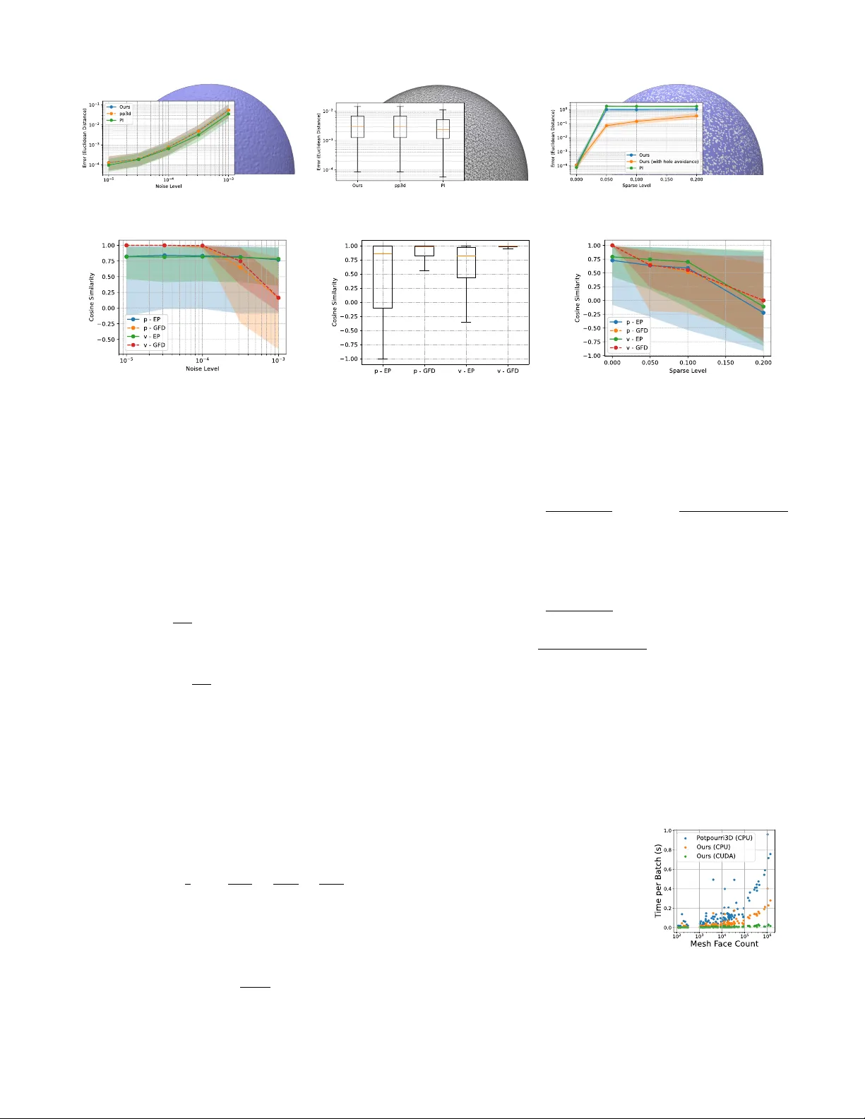
Parallelised Differ entiable Straightest Geodesics for 3D Meshes Hippolyte V erninas Caner K orkmaz Stef anos Zafeiriou T olga Birdal * Simone Foti * Imperial College London Abstract Machine learning has been pr o gr essively gener alised to op- erate within non-Euclidean domains, but geometrically ac- curate methods for learning on surfaces ar e still falling be- hind. The lack of closed-form Riemannian operators, the non-differ entiability of their discr ete counterparts, and poor parallelisation capabilities have been the main obstacles to the de velopment of the field on meshes. A principled fr ame- work to compute the e xponential map on Riemannian sur- faces discretised as meshes is straightest geodesics, which also allows to tr ace geodesics and parallel-tr ansport vec- tors as a by-pr oduct. W e pr ovide a parallel GPU imple- mentation and derive two differ ent methods for differ enti- ating thr ough the straightest geodesics, one le vera ging an extrinsic pr oxy function and one based upon a g eodesic fi- nite differ ences scheme. After pr oving our parallelisation performance and accur acy , we demonstr ate how our differ - entiable exponential map can impr ove learning and opti- misation pipelines on gener al geometries. In particular , to showcase the versatility of our method, we pr opose a new geodesic con volutional layer , a new flow matching method for learning on meshes, and a second-or der optimiser that we apply to centroidal V or onoi tessellation. Our code, mod- els, and pip-installable library ( digeo ) are available at: cir cle-gr oup.github .io/resear ch/DSG . 1. Introduction What do molecules, proteins, the Earth, joint articulations, orthonormal matrices and a spaceship (like the one in Fig. 1 ) hav e in common? They all have fundamental properties that can be modelled through Riemannian geometry . T remen- dous progress has recently been made possible by integrat- ing the geometry of these spaces into learning [ 7 , 9 , 34 , 38 , 58 , 85 , 87 ] and by the av ailability of software libraries providing Riemannian operators for analytically defined spaces admitting closed-form-solutions [ 43 , 54 , 55 , 81 ]. Significant ef forts have also been made to learn on sur- faces [ 11 , 14 , 26 , 52 , 65 , 67 , 75 ], but when Riemannian * Joint senior authors, equal contribution G e o d e s i c F i n i t e D i f f e r e n c e s f o r v G e o d e s i c F i n i t e D i f f e r e n c e s f o r p E x t r i n s i c P r o x y Figure 1. Our GPU-parallelised schemes to dif ferentiate the Ex- ponential map and improve learning and optimisation on meshes: the Extrinsic Proxy (EP) and Geodesic Finite Dif ferences (GFD). operators are needed, they are pre-computed [ 52 , 65 ], or re- placed by slo w numerical solvers [ 14 ]. In this work, we take an important step to wards enabling the adoption of Rieman- nian operators directly into learning and optimisation meth- ods for meshes. W e focus on developing a differentiable exponential map, arguably the most important Riemannian operator, a function that takes a tangent vector at a starting point and finds the end point of the geodesic traced according to that vector . While closed-form solutions of the exponential map exist for simple canonical shapes like spheres [ 45 ], more complex shapes require the use of advanced computational techniques. On dscrete surfaces, tracing the geodesic curve that determines the solution of the exponential map re- quires numerically solving the initial v alue problem, a sys- tem of second order differential equations, later detailed in Sec. 3 . Unfortunately , this approach not only is rather cum- bersome [ 15 ], but also computationally inefficient and pri- marily suited for smooth continuous surfaces. In comput- ing, most surfaces are discretised into meshes and different techniques are needed [ 15 , 19 , 64 ]. T o date, the straightest geodesics method introduced in [ 64 ] is the de-facto choice for computing the e xponential map and geodesic tracing on triangular meshes. All available implementations are non- differentiable and conceiv ed to operate sequentially on the CPU. Consequently , the existing formulation of the expo- nential map is not suitable for integration within modern learning and optimisation framew orks for 3D meshes. W e deriv e two dif ferent implementations of the dif feren- 1 tial (Fig. 1 ): a faster version using an extrinsic proxy (EP) and a slower yet more accurate geodesic finite-differences (GFD) scheme. EP uses a proxy function to emulate the tracing result in Euclidean space, thus providing an analyt- ical formulation that can be easily differentiated. GFD is based upon finite dif ferences, which we adapt to respect the geometry of the mesh. Both schemes are agnostic to the forward computation of the exponential map, and can pro- vide differentiability to any exponential map. Additionally , we propose a parallel GPU implementation of the straight- est geodesics that can handle tens of thousands of points on multiple meshes, yielding results in just a few milliseconds. W e thoroughly benchmark the speed and accuracy of both our forward and backward step against existing implemen- tations and closed-form exponential maps. Then, we focus on demonstrating our methods by proposing three ne w competitive applications. W e intro- duce a nov el geodesic conv olution that dynamically learns the patch size during training. Our conv olution outperforms fixed-patch methods and most leading intrinsic techniques. W e then propose a flow matching-inspired method for arbi- trary meshes that reduces inference time by orders of mag- nitude while using a fraction of GPU memory , and outper- forming the state-of-the-art. Finally , we introduce a second order LBFGS-based [ 36 , 66 ] Riemannian optimiser for 3D meshes that we use for computing the centroidal V oronoi tessellation [ 22 ]. Also in this case our method achieves faster con ver gence and superior minimisation performance. It is worth noting that beyond our proposed applications, we expect our contributions to benefit a wide variety of domain- specific applications. T o summarise, our key contrib utions are: 1. A differentiable straightest geodesics method to com- pute exponential maps, trace geodesics, and parallel- transport vectors on the surface of 3D meshes that is ef- ficiently parallelised on the GPU. 2. A PyT orch-compatible software library featuring C++ CUD A kernels that enables seamless integration of discrete Riemannian geometry into modern learning pipelines for meshes. 3. Adaptive Geodesic Conv olutions (A GC) that learn their patch size for each channel and layer . 4. MeshFlow , a ne w flow-matching-inspired method based on our exponential map and optimal transport. 5. Mesh-LBFGS , a second order LBFGS optimiser for meshes that we use to efficiently solve the centroidal V oronoi tesselation problem. 2. Related W ork Numerous existing works on geodesics has focused on solv- ing the Boundary V alue Problem (BVP) to compute the shortest paths between two points on a discrete surface [ 3 , 12 , 17 , 18 , 37 , 39 , 46 , 57 , 60 , 80 ]. Widely researched are also algorithms for computing the logarithm map and cre- ate local parametrisations [ 35 , 72 , 74 , 77 ], which are par- ticularly useful for texturing. As noted in [ 77 ], the graph- ics community has often misused the logarithm and expo- nential map terminology . W e here adhere to the Rieman- nian geometry definitions. Therefore, when looking at the IVP literature for tracing straightest geodesics and comput- ing the exponential map, we note that it is quite prolific on continuous surf aces and considerably under -explored on meshes. Iterativ e integration of the IVP ODE [ 86 ] is possi- ble on smooth continuous surfaces, but computationally in- efficient. For this reason, closed-form solutions are always preferred when av ailable, lik e on SO(3) [ 34 , 87 ], SE(3) [ 9 ], or the sphere [ 14 , 53 ]. These and other equally well-defined simple spaces are readily av ailable in famous libraries for Riemannian geometry [ 43 , 54 , 55 , 81 ]. On meshes, [ 64 ] still represents the gold standard. The isolated attempt to improve [ 64 ] by approximating the con- tinuous surface discretised by the mesh is more compu- tationally expensiv e, still non-differentiable, and produces off-mesh results. Beyond meshes, [ 28 ] extended exponen- tial maps to implicit functions. Its approximate nature and a mandatory representation con version mak e it unsuitable for meshes. Finally , [ 50 ] introduced a representation-agnostic exponential map obtained through an iterativ e projection from the tangent space. Howe ver , their step-size selection imposes a critical trade-off between accurac y and speed. 3. Riemannian Geometry In this section we pro vide a self-contained summary of the Riemannian geometry concepts related to our work and rec- ommend [ 32 , 45 ] for a broader revie w of the field. Let M ⊂ R 3 be a Riemannian manifold embedded in 3D Euclidean space and T M = S p ∈M T p M be the tangent bundle set encompassing the tangent spaces of all points p on M . By definition, a manifold M is locally homeomor- phic to T p M ⊂ R 3 . A curv e γ : I → M parametrised over an interv al I = [ a, b ] (with a, b ∈ R ), is a geodesic on a smooth Riemannian surface when it can be simultaneously characterised as being the shortest and straightest. Since for triangular meshes straightest and locally shortest geodesics differ from each other [ 64 ], and this work focuses on the for- mer , we here define geodesics according to the straightness criteria also in the continuous setting. T o define straightness we need a way to characterise the absence of intrinsic cur- vature. In R 3 we would just impose ¨ γ = 0 , but if we attempt to write ¨ γ as lim ∆ t → 0 ˙ γ ( t +∆ t ) − ˙ γ ( t ) ∆ t it becomes immediately obvious that the tangent vectors ˙ γ ( t + ∆ t ) and ˙ γ ( t ) cannot be directly compared as they belong to two different tan- gent planes, T p 1 M and T p 0 M , with p 1 = γ ( t + ∆ t ) and p 0 = γ ( t ) . Therefore, to correctly compute this second deriv ativ e we need to take into account how tangent vec- tors ˙ γ ( t ) turn as they move along the tangent direction ˙ γ ( t ) . 2 This can be achie ved with the Co variant deriv ativ e, which is usually computed using the metric preserving and torsion- free Le vi-Civita connection ∇ . The Riemannian equiv a- lent of ¨ γ = d 2 γ ( t ) dt 2 = d dt ˙ γ ( t ) can therefore be rewritten as ∇ ˙ γ ( t ) ˙ γ ( t ) and it equals zero ∀ t ∈ [ a, b ] if γ ( t ) is a geodesic. This intrinsic formulation could also be reframed from an extrinsic point of view by allo wing γ to hav e curv ature only in the normal direction of M . A fundamental problem in Riemannian geometry is to identify the unique geodesic curve γ v ( t ) : [ a, b ] → M originating in p ∈ M given an initial tangent velocity v ∈ T p M . This amounts to solving the initial value prob- lem (IVP) represented by the following second order system of ordinary differential equations: γ v ( t ) =      ∇ ˙ γ ( t ) ˙ γ ( t ) = 0 γ ( a ) = p ˙ γ ( a ) = v (1) The exponential map Exp p : T p M → M is the map that computes the end-point of the geodesic obtained by solv- ing the IVP . In other words, given p ∈ M and a vector v ∈ T p M , the exponential map determines the point on the manifold obtained walking until the end of the geodesic originating in p with direction v ∥ v ∥ and length ∥ v ∥ . There- fore we have: Exp p ( v ) = γ v ( b ) . The in verse of the expo- nential map is called logarithm map and is defined over a neighbourhood N ( p ) of p ∈ M where Exp p is inv ertible. Giv en any point p ′ ∈ N ( p ) , Log p : N ( p ) ∈ M → T p M finds the shortest vector v such that Exp p ( v ) = p ′ . As previously mentioned, the Le vi-Ci vita connection provides a rule for comparing tangent v ectors at differ - ent points, thereby defining the notion of parallel trans- port . A vector field along γ is a smooth map W γ : I → T γ ( t ) M and is considered parallel if it is cov ariantly con- stant: ∇ ˙ γ ( t ) W γ = 0 . When ∇ is Le vi-Civita, for every C 1 curve γ , any t 0 ∈ I , and any initial vector w ∈ T γ ( t 0 ) M there exists a unique parallel v ector field W γ satisfying the initial condition W γ ( t 0 ) = w . Given { t 0 , t 1 } ∈ I , the parallel transport of w along γ from t 0 to t 1 is thus writ- ten as Q t 1 γ ,t 0 = W γ ( t 1 ) and is computed by simultaneously solving the system of dif ferential equations for the geodesic curve (Eq. ( 1 )) and the parallel v ector field therein defined. 4. Differentiable Straightest Geodesics After detailing the computation of γ v , Exp p ( v ) , and Q t 1 γ ,t 0 on meshes using straightest geodesics [ 64 ], we introduce our two methods for differentiating through Exp p ( v ) and our GPU parallelisation strategy . Our differentiable and ef- ficient operators build the foundations for a differentiable Riemannian geometry stack on meshes. Instead of continuous manifolds M we now consider meshes M = { X , F } , with X ∈ R N × 3 = [ x 1 . . . x N ] T representing the N vertices x i = [ x i , y i , z i ] ⊤ , and F ∈ N F × 3 the F triangular faces. V alues in each f i ∈ F in- dex the vertices to define the mesh’ s connectivity . The mesh is manifold if each edge is incident to either one or two faces, and faces around each vertex form a single connected f an. Points on the surface of M are defined by the pair (f , b ) , where f ∈ N is the index of the face on which a point lies, and b = [ b u , b v , b w ] T its barycen- tric coor dinates on f . These coordinates belong to the 2- simplex Σ 2 =  b ∈ [0 , 1] 3 | P k =( u,v ,w ) b k = 1  . Giv en x 0 , x 1 , x 2 as the vertices of f f , the coordinates of p ∈ M are p = b u x 0 + b v x 1 + b w x 2 , where b w = (1 − b u − b v ) according to the definition of Σ 2 . Straightest geodesics . Giv en a point p ∈ M and a vector v ∈ T p M , the straightest geodesic algorithm uses the angle preservation criteria (Fig. 2 ) to iterativ ely trace a geodesic γ v from one face onto another . Like in the continuous set- ting Exp p ( v ) = γ v ( b ) . start θ l θ r fini sh Figure 2. Left θ l and right θ r an- gles on a verte x, edge, and face. The discrete analogue to imposing ∇ ˙ γ ( t ) ˙ γ ( t ) = 0 is to impose left and right curve angles ( θ l , θ r ) to be the same for every p along γ ( t ) [ 64 ]. θ l and θ r are the angles that incoming and outgoing segments of the curve γ form with the total angle space θ ( p ) at point p . While the straightness condition is θ l = θ r , ∀ p ∈ M , we need to distinguish how the total angle definition changes in the three separate cases depicted in Fig. 2 : when a point is within a face, on an edge, or on a vertex. For all points within faces we are ef fectiv ely on a plane, so the total angle is θ ( p ) = 2 π . Considering that two connected faces can easily be made coplanar , the neighbourhood of a point on an edge is isometric to a plane and thus θ ( p ) = 2 π also for all points on edges. For vertices, on the other hand, the total angle is the sum of all interior angles of the m faces meeting at the vertex: θ ( p ) = P m i =1 θ i ( p ) . Therefore, at vertices, θ ( p ) = 2 π if all faces connected to the vertex are coplanar , θ ( p ) < 2 π for spherical (cone-like) vertices, and θ ( p ) > 2 π for hyperbolic (saddle-like) vertices. Further details on the implementation of the geodesic step are pro- vided in Alg. A.1 . The approach exploits the extrinsic ge- ometry to accelerate computations, relying on the normal vectors of faces and v ertices. This does not pose any disad- vantage, since 3D meshes are almost al ways embedded in a Euclidean space with a canonical frame. Note that the original algorithm of [ 64 ] stops tracing geodesics when reaching the boundary of the mesh ∂ M (i.e., when reaching an edge incident only to one face or a v ertex belonging to it) ev en if the desired length | v ∥ is not reached. While correct, we notice that this behaviour can negati vely affect performance during learning and optimi- 3 sation in the presence of small holes and defects (Sec. A.7 ). W e thus give the option to temporarily interrupt the straight- ness criteria, trace along the boundary , and resume trac- ing as soon as possible with the last straightest direction recorded when ∂ M was reached. Parallel T ransport can be defined via the discrete equiv- alent of ∇ ˙ γ ( t ) W γ = 0 , which corresponds to imposing the normalised angle α between the vector field W γ and the curve’ s tangent vector ˙ γ ( t ) to be constant ∀ t ∈ I , with α  W γ ( t ) , ˙ γ ( t )  := 2 π θ ( p ) ∠  W γ ( t ) , ˙ γ ( t )  [ 64 ]. Giv en { t 0 , t 1 } ∈ I , the parallel transport of w along γ from t 0 to t 1 , Q t 1 γ ,t 0 , is obtained while iterativ ely tracing the geodesic. When crossing vertices W γ ’ s orientation is corrected ac- cording to α . When crossing an edge, W γ ’ s orientation is simply maintained relative to the unfolded plane because θ ( p ) = 2 π and the normalised angle is then identical to the Euclidean angle ∠ . Differentiation . As shown in [ 13 ], automatic differenti- ation in Riemannian settings is problematic in nature be- cause naiv e Euclidean gradients produce off-manifold re- sults. Furthermore, the piecewise linear nature of straight- est geodesics on M results in a discontinuous deriv ative ( ˙ γ v ( t ) / ∈ C 1 at face transitions), which inherently prev ents automatic back-propagation through Exp p ( v ) and makes its adoption in optimisation or learning problems infeasible without an explicit differentiation scheme. More details on non-differentiability are pro vided in Sec. A.1 . Giv en a composite function, h ( z ) = f (Exp( g ( z ))) = y , sending an input z ∈ R n z to y ∈ R n y , we hav e: h : R n z g − − − → ( M × T M ) Exp − − − → M f − − − → R n y . (2) h ( z ) represents the general scenario in which Exp is used within a more complex frame work in v olving other dif feren- tiable functions f and g , which could also be parametrised by neural networks. If we need to differentiate through h we can use the chain rule. Indicating with J ∈ R m × n the Jacobian matrix whose ro ws are the m transposed gradients ( ∇ ∈ R n ) of the function’ s m output components, we hav e: J h = J f ·  J p Exp · J p g + J v Exp · J v g  , (3) where each Jacobian is computed with respect to the input of the function it is referred to. If a function has either mul- tiple inputs or multiple outputs, the superscript is used to select a specific input/output sub-block of the full Jacobian. If a function is not used, its Jacobian is the identity matrix, making the formulation of h valid also when f and g are not used. When a loss function L is computed on y = h ( z ) , the full chain rule becomes ∇ z L = ∇ y L · J h ( z ) . Nev ertheless, what emerges from Eq. ( 3 ) is that we need J v Exp and J p Exp to enable full differentiability of Exp p ( v ) . Refer to Fig. 1 and the corresponding insert figures for a visual description of all the differentiation schemes detailed hereafter . Differentiation via Extrinsic Proxy (EP) . The first of our two proposed dif ferentiation schemes uses a proxy func- tion φ ( p , v ) that le verages Exp( p , v ) —computed with the non-differentiable straightest geodesics method— to define a proxy endpoint p ′ proxy (= p ′ ) that we can dif ferentiate. In particular , φ is defined as: φ ( p , v ) = p ′ proxy =  R fix · ( p + v )  + t fix . (4) Here, ( p + v ) is the Euclidean mov ement of p according to v . R = M T p M p ′ represents the total cumulativ e rotation accu- mulated by the geodesic path as it tra vels along the curved surface and acts as a dif feren- tiable surrogate for parallel transport in Euclidean space. It is computed as the rotation between the orthonormal frames defined at the start and end of the geodesic. Here, the ax es of the starting frame M p (and columns of the matrix) are: ˆ e ∥ = v ∥ v ∥ , ˆ e ⊥ = ˆ n × ˆ e ∥ , and ˆ n —which is the normal to the tangent plane where v is defined. M p ′ is built follo wing the same procedure, b ut replacing v with its parallel trans- ported version in p ′ , which we indicate as Q p ′ p ( v ) using a small abuse of notation to improve clarity in the discrete setting. Finally , t = p ′ − R · ( p + v ) is the fixed bias trans- lation v ector that forces φ to perfectly match the position of p ′ and the “fix” superscript indicates a gradient detachment. Note that the extrinsic proxy is specifically constructed to model differential changes of v . In fact, if we differenti- ate φ with respect to v we obtain J v Exp = R fix · I . Therefore, in the backward pass, R fix backward parallel transports the upstream Jacobian (e.g. J f in Eq. ( 3 )) from p ′ to p . Unfor- tunately , if we differentiate φ with respect to p , the result is unchanged, showing that changes in the initial position would also be treated as rigid rotations while completely ignoring how the geodesic shifts when its starting point p changes. Observing Eq. ( 3 ), it becomes obvious that this incorrectness can jeopardise the optimisation e ven for prob- lems that seek to optimise only with respect to the v com- ponent of Exp( p , v ) . Therefore, we void the contributions of p by zeroing the elements of J p Exp . Instead of computing the proxy and letting autograd differentiate φ , we directly use Exp in the forward step and use the manually computed Jacobian of φ in the backward step. Differentiation via Geodesic Finite Differences (GFD) . T o introduce our finite differences scheme, we first define the local reference frames of our intial conditions. For vectors v in the tangent bundle we use ˆ e ∥ and ˆ e ⊥ , as de- fined for the EP differentiation approach. For points, we define a non-orthogonal barycentric coordinates system as ˆ e u = x 1 − x 0 ∥ x 1 − x 0 ∥ and ˆ e v = x 2 − x 0 ∥ x 2 − x 0 ∥ . This system is consis- tent with the barycentric definition of points and simplifies perturbations for finite differences. Since it is still defined 4 in the tangent of a face, it also allo ws to project from ambi- ent space ( R 3 ) onto the local frame M = [ ˆ e u ˆ e v ] ∈ R 3 × 2 by using its pseudoinv erse (Moore–Penrose inv erse) M † = ( M T M ) − 1 M T . Giv en an extrinsically defined p and a vector v in its local reference sys- tem, we hav e J v Exp ∈ R 2 × 2 , where columns correspond to perturbations along the axes of the local reference system. In order to apply a for - ward finite dif ferences scheme we need to introduce pertur- bations along the axes of v ’ s frame and project the Jacobian in ambient space to the local frame: J v Exp ≈ M † p ′ · h Exp( p , v + ε v ˆ e ∥ ) − p ′ ε v Exp( p , v + ε v ˆ e ⊥ ) − p ′ ε v i (5) where ε v is a small constant and M † p ′ is the projection per- formed on the barycentric frame at p ′ = Exp( p , v ) to project the finite differences to the same coordinate sys- tem. Note that the perturbation along ˆ e ∥ is aligned with the direction of v and is equiv alent to increasing the length of the trace by ε v . Therefore, instead of computing the full Exp( p , v + ε v ˆ e ∥ ) , we can trace a significantly shorter geodesic from p ′ with initial vector equal to the paral- lel transported incremental displacement. In other words Exp( p , v + ε v ˆ e ∥ ) = Exp  p ′ , Q p ′ p ( ε v ˆ e ∥ )  . The procedure to ob- tain J p Exp is very simi- lar , but a perturbation of p in its barycentric system may move the origin of the geodesics onto new faces. Therefore, we also need to compute the ne w starting points and their corresponding parallel-transported starting vectors. W e first perturb p and compute p u = Exp( p , ε p ˆ e u ) and p v = Exp( p , ε p ˆ e v ) , as well as their parallel transported directions v u = Q p u p ( v ) and v v = Q p v p ( v ) . Then, we hav e: J p Exp ≈ M † p ′ · h Exp( p u , v u ) − p ′ ε p Exp( p v , v v ) − p ′ ε p i . (6) Parallelisation on the GPU . T o efficiently compute Exp( p , v ) for large batches, we parallelise the tracing algo- rithm on the GPU. The core design principle is to le verage the independence of each geodesic path. W e launch a single CUD A kernel where each thread is responsible for tracing one complete geodesic path from a starting point p with an initial vector v (Alg. 1 ). Each thread ex ecutes its own trac- ing loop, iterativ ely advancing the point across the mesh faces as described in Sec. 4 . This one-thread-per-geodesic strategy naturally accommodates paths of varying complex- ity and length. Threads assigned to shorter geodesics (i.e., Algorithm 1 Parallel Geodesic T racing CUDA K ernel In: M (mesh); P , V (batch of start points and v ectors) Out: P ′ , V ′ (batch of end points and vectors) i ← threadIdx.x + blockIdx.x × blockDim.x if i ≥ length ( P ) then return p ← P [ i ] ; v ← V [ i ] ( v , p ) ← initialise trace ( M , p , v ) L target ← ∥ v ∥ ; L traced ← 0 ; step ← 0 while L traced < L target and step < MAX STEPS: ( p , v , L step ) ← geodesic step ( M , p , v ) L traced ← L traced + L step ; step ← step + 1 P ′ [ i ] ← p ; V ′ [ i ] ← v 10 4 10 3 10 5 10 6 0.30 200 50 25 0 0.20 0.10 0.00 10 3 2 4 (16) 2 6 2 8 2 10 2 12 2 14 2 16 ( ˜ 66k) 10 2 10 1 10 0 10 - 1 10 - 2 10 - 3 P oin ts B atc h Size M es h F ace Coun t Tim e p er B atc h (s) PI (GPU) p p3d (CPU) geometry-cen tra l (CPU) Ours (CPU/C++) Ours (GPU/CUD A) Figure 3. Median runtime comparisons with different batch sizes ( left ) and face counts ( right ). Medians are computed ov er 5 con- secutiv e executions (as well as 5 different meshes for the left ). While variance is negligible with face counts, 25% and 75% in- tervals are reported for batch sizes. The time axis was split in right to highlight the massive performance gap with PI. smaller ∥ v ∥ ) or simpler paths will complete their while loop and write their result, becoming idle sooner . Meanwhile, threads tracing longer or more complex paths (e.g., cross- ing many vertices) continue executing. This model avoids complex inter-thread synchronisation. The GPU’ s stream- ing multiprocessors remain saturated with activ e warps trac- ing the remaining paths, ensuring high utilisation until the longest path in the batch is complete. Since the tracing algorithm only depends on the lo- cal faces, it can also simultaneously process meshes het- erogeneously batched together . Ensuring that the indices within face matrices ( F ) and intrinsically defined points P = { (f , b ) } are correctly of f-setted for each M is the only additional step required for parallelising across meshes. 5. Experimental Evaluation & Applications W e report the accuracy and performance of our method in both its forward and backward steps in Sec. 5.1 . Then, we present our three nov el applications in Secs. 5.2 to 5.4 . 5.1. Accuracy & Performance W e test our Exp across the three back-end implementa- tions we provide (Python, C++, and CUDA) against the SotA implementations of [ 64 ] provided by the C++ li- brary geometry − central [ 73 ] and its Python wrapper potpourri3d ( pp3d ). W e test on 5 different meshes (Fig. A.1 ) with a div erse face count in the approximate range of F ∈ [200 , 1 . 7 M ] and report accuracies comparable 5 T able 1. Comparison of Accuracy Metrics. Left : mean distances between the endpoints of our different backends and pp3d . Right : mean distances against the Exp map of the sphere and torus. python C++ CUD A float32 2 . 0 e-5 2 . 0 e-5 2 . 0 e-5 float64 7 . 1 e-9 1 . 0 e-9 1 . 0 e-9 Ours pp3d PI [ 50 ] Sphere 5 . 7 e-4 5 . 7 e-4 5 . 4 e-4 T orus 8 . 9 e-3 8 . 9 e-3 8 . 9 e-3 to pp3d (T ab . 1 , left ), while being 3 or ders of magnitude faster on big batch sizes (Fig. 3 , left ). Our CUD A imple- mentation also scales linearly with the number of faces of a mesh, consistently outperforming by 2 order s of magnitudes other methods (Fig. 3 right ). Our CUDA implementation also has nearly constant run-times while scaling either of those factors on a single NVIDIA R TX-4090. As reported in T ab . 1 ( right ), both ours and pp3d ’ s Exp report similar performance on the closed-form exponen- tial map of the sphere Exp sphere ( p , v ) = p cos( ∥ v ∥ ) + v ∥ v ∥ sin( ∥ v ∥ ) and the exponential map computed by solv- ing the IVP on a torus (properly formulated in Sec. A.4 ). Errors are here mostly caused by discretisation and the y de- crease as resolution increases and the mesh becomes a better approximation of the underlying continuous surface. Cos ine sim ilarit y A ccuracy EP PI GFD 1.0 -1.0 0.5 0.0 -0.5 1.0000 0.9996 0.9999 0.9998 0.9997 Figure 4. Differentiation correct- ness against closed-form. The accuracy of our two dif ferentiation schemes is tested against closed- form gradients computed on the sphere (Fig. 4 ), which we deriv e in Sec. A.3 . Our GFD scheme closely matches the gradients on the sphere for both v and p . Results for our EP schemes corroborate our mathematical deriv ation by showing that gradients for v are a good ap- proximation of the real ones, with their norm being par- ticularly reliable. In addition, it also shows that the gra- dients for p are not reliable, further motiv ating our choice for voiding their contributions. Our experiments sho w that the backward pass with GFD is about 3.85 times more ex- pensiv e than with EP . Overall while GFD should be the de- fault choice for most applications, EP is preferable for ap- plications requiring fast computations of gradients for v and where p are fixed (e.g., Sec. 5.2 ). The projection integration (PI) we reproduced from [ 50 ] exhibits similar accurac y to ours (T ab . 1 , right ), but we are a staggering 5 to 6 or ders of magnitude faster on meshes with a high face count and large batches, respectiv ely (Fig. 3 ). Note that PI can be auto-differentiated, but gradients (and speed) are of insufficient quality for optimisation (Fig. 4 ). 5.2. Adaptive Geodesic Con volutions (A GC) Problem & Setup . Geodesic Conv olutional Neural Net- works (GCNN) [ 52 ] extend the con volution operation to manifolds by replacing the Euclidean metric with geodesic distances defined on the surface. Most follo w-up works [ 8 , 52 , 56 , 65 , 84 ] tried to o vercome the absence of a local coordinate system. Nevertheless, a ke y limitation remains: their reliance on a fix ed patch size, typically determined by precomputing geodesic distances or aggregating a predeter- mined set of neighbouring vertices. This rigid definition limits the model’ s ability to adapt to local geometry . Appr oach . T o address this, we propose leveraging our dif- ferentiable straightest geodesics to dynamically learn patch sizes during training. This allows the recepti ve field to ad- just based on the underlying surface geometry , resulting in a more flexible and expressi ve model capable of capturing features at the most relev ant scales. Note that unlike Diffu- sionNet [ 75 ], which also learns kernel’ s sizes for different channels, our filters are not curvature dependent —a side ef- fect of using the Laplace Beltrami Operator to diffuse heat. W e define a set of planar vectors by rotating an arbitrary base versor ( ˆ v base ) n θ times while modulat- ing its length with n ρ different values: v k,l = k ρ w R ( θ l ) ˆ v base for k = 1 ...n ρ , l = 1 ...n θ . V alues defined at the end-points of these vectors and their origin determine the learnable filter v alues w c l,k and w c i , respecti vely . T o apply filters, we first find the corresponding points on the surface p ′ k,l = Exp x i ( v k,l ) ∈ M and then barycentrically interpolate the values at the ver- tices of the faces on which the p ′ k,l belong. If we represent the interpolation of vertex feature Y κ c at layer κ and channel c with B ( Y κ c , Exp x i ( v k,l )) , we hav e: Y κ +1 i,c = Y κ i,c w c i + max π n θ X l =1 n ρ X k =1 w c π ( l ) ,k B ( Y κ c , Exp x i ( v k,l )) . Rotational in variance is achiev ed by cyclically permuting angular indices with π ( l ) , effecti vely rotating the filters. T o speed up computations, filters are grouped in ν subsets sharing the same { v k,l } . Thanks to our differentiable Exp , along the filter values we also learn one ρ w for each subset of filters. Since we are optimising only the norm of the vec- tor directions, we use the EP differentiation scheme, which is much faster to compute and quite accurate when optimis- ing with respect to the norm of the direction vector . Our network takes as input a vector of real values for each verte x. Like in Dif fusionNet [ 75 ], we considered two possible input types: the raw 3D coordinates of the vertices, and the Heat K ernel Signature (HKS) [ 79 ]. More details on our model and training setup are provided in Sec. A.6 . Results . W e trained our A GCNN to segment the hu- man body parts on the composite dataset [ 51 ], contain- ing models from sev eral other human shape datasets [ 1 , 2 , 6 , 29 , 83 ]. W e trained our model on the orig- 6 T able 2. Body part segmentation accuracy . XYZ and HKS denote position coordinates and heath kernel signatures as inputs. ∗ indi- cates models trained on a modified dataset for verte x predictions. Method Accuracy GCNN [ 52 ] 86.4% MDGCNN [ 65 ] 89.5% HSN* [ 84 ] 91.1% FC* [ 56 ] 92.9% DiffusionNet - XYZ [ 75 ] 90.6% DiffusionNet - HKS [ 75 ] 91.7% A GC (Ours) - XYZ 91.7% A GC (Ours) - HKS 92.3% inal dataset, predicting faces, by summing the logits of the face vertices. When using HKS as input, the model con verges faster and reaches a higher accuracy . Figure 5. A GC (ours) on body parts segmentation. Fig. 5 depicts some segmenta- tions performed with our model, while T ab . 2 reports a compari- son against SotA methods using geodesic con volutions on meshes. Even though our model is just an extension of GCNN [ 52 ], it brings significant impro vements over other methods and partic- ularly over our closest competitors (i.e., GCNN [ 52 ] and MDGCNN [ 65 ]). The only model outperforming A GC was trained to predict vertex rather than face classes, making the comparison only partially fair . W e trained our model on a Nvidia A100, taking 1 minute and 21 seconds per epoch and using around 6 . 8 GB of VRAM, while training on the full size meshes made of around 10 k vertices. The GFD scheme, took around 2 minutes and 8 seconds per epoch and 7 . 2 GB of VRAM, for similar accuracy . Our con volution layer is currently inspired by GCNN [ 52 ], which is one of the earliest and simplest mesh con volutions. As future study , we imagine adapting MDGCNN [ 65 ] or FC [ 56 ] to use adaptiv e patch sizes like in AGC. Interestingly , by dropping the max pooling like in MDGCNN [ 65 ] and learning a different ρ k for each angle, it would also be possible to learn anisotropic filters. 5.3. MeshFlow Problem & Setup . Flow Matching [ 48 ] is a recent ap- proach to constructing normalising flows [ 20 , 21 , 31 , 41 , 42 , 61 , 62 , 68 ] by directly learning a vector field that trans- ports one distribution onto another without requiring like- lihood computation through an ODE solver . Riemannian flow matching (RFM) [ 14 ] generalises this framework to Riemannian manifolds by learning time-dependent tangent vector fields v t,θ ( p ) ∈ T p M and moving points geodesi- cally . Unlike on the simple manifolds, [ 14 ] requires solving an ODE to identify a geodesic path on meshes. Since the Euler solver they use can drift of f the surface, an additional projection step is required. Thanks to our dif ferentiable in- trinsic method we can av oid both steps and directly learn the GT RFM Ours Bunny ( k =10) Bunny ( k =50) Bunny ( k =100) Spot ( k =10) Spot ( k =50) Spot ( k =100) Figure 6. Comparison of eigenfunctions (GT), RFM predictions and our predictions on Bunny and Spot for dif ferent values of k . vector field by back-propagating through Exp . Therefore, our time-independent vector field does not need to match the marginal v ector field of RFM. Differences and similari- ties between the two methods are detailed in Sec. A.7 . Appr oach . Rather than parametrising and optimising a time-dependent vector field, we instead learn a single sta- tionary vector field defined on the manifold. The gener- ativ e process is constructed by transporting samples from the base to the target distribution using pointwise corre- spondences obtained via optimal transport (OT). The trans- port cost is defined as the squared biharmonic distance [ 47 ], which serves as a computationally efficient surrogate for the true geodesic distance. W e can then use the learned vector field to move the samples to the target distribution. Since we are using exponential maps, there are no projection errors, making the method useable with a low amount of steps, while still maintaining high accuracy . Our objectiv e is: L ( θ ) = E p i ∼U ( M ) q i ∼Q ( M ) " B X i =1 d 2 BH  Exp ⟳ K p i ( v θ ) , q σ ( i )  # , (7) where p i ∈ M are initial samples from a uniform dis- tribution over the mesh U ( M ) , q i are samples from the target distribution Q ( M ) , d BH is the biharmonic distance, σ is a permutation of [1 , B ] representing the OT coupling for the batch, and Exp ⟳ K is the K -steps exponential map breaking the trajectory into multiple steps and enabling non- straightest curves on M . In practice, it iterati vely computes p ( k +1) i = Exp p ( k ) i  v θ ( p ( k ) i ) /K  for k = 0 , . . . , K − 1 , thus allowing changes in direction by re-ev aluating the learned v ector field at intermediate points. T o learn the vec- tor field, we use a MLP with 3 hidden layers of size 512 , and K = 5 . The MLP takes as input the 3D position of the samples and outputs the corresponding vector . W e use the GFD differentiation scheme as we need to back-propagate also through positions. Full details in Sec. A.7 . Results . Like [ 14 , 71 ], we use the eigenfunctions of the Stanfor d Bunny [ 82 ] and Spot [ 16 ] as ground truth target distributions. W e report qualitative and quantitativ e com- parisons in Fig. 6 and T ab . 3 , respectively . Our method 7 T able 3. Flow matching test metrics for different eigenv ectors. ∗ NLL is unreliable when comparing to RFM (see Sec. 5.3 ). Metric Method Stanford Bunny Spot the Cow k =10 k =50 k =100 k =10 k =50 k =100 RFM [ 14 ] 1.22 1.44 1.55 1.03 1.14 1.26 NLL ∗ ( ↓ ) MeshFlow-256 (ours) 1.49 1.74 1.75 1.34 1.42 1.38 MeshFlow-1024 (ours) 1.48 1.73 1.71 1.26 1.38 1.32 RFM [ 14 ] 0.050 0.11 0.13 0.087 0.065 0.084 KLD ( ↓ ) MeshFlow-256 (ours) 0.090 0.072 0.13 0.15 0.094 0.055 MeshFlow-1024 (ours) 0.060 0.036 0.058 0.050 0.044 0.034 RFM [ 14 ] 0.014 0.018 0.020 0.013 0.014 0.014 BCD ( ↓ ) MeshFlow-256 (ours) 0.016 0.018 0.021 0.015 0.015 0.016 MeshFlow-1024 (ours) 0.015 0.015 0.017 0.012 0.013 0.013 reports superior results on both KL diver gence (KLD) and biharmonic-based Chamfer distances (BCD), which is the only geodesic measure. While we yield a higher negati ve log likelihood (NLL), this metric is inherently tied to the optimisation objecti ve, making the NLL comparison infor- mativ e only across the two variants of MeshFlo w , which exhibits improvements when using more samples to com- pute the O T couplings. Our method is also 1 . 6 · 10 4 times faster during inference, and uses 97% less GPU memory compared to RFM. W e provide more details in Sec. A.7 . 5.4. Mesh-LBFGS optimiser Problem & Setup . The Broyden-Fletcher -Goldfarb- Shanno (BFGS) method [ 59 ] is a classical quasi-Ne wton algorithm for unconstrained smooth optimisation. Quasi- Newton methods iterati vely approximate the in verse Hes- sian of the objecti ve function, thereby capturing curva- ture information without computing second deriv ativ es ex- plicitly . Howe ver , the main drawback of the classical BFGS method is its storage cost. L-BFGS [ 49 ] av oids ex- plicit storage, instead retaining only the most recent up- dates to gradient and position dif ferences. L-BFGS has become one of the most widely used large-scale optimisa- tion algorithms and was adapted to Riemannian optimisa- tion in [ 4 , 36 , 69 , 88 ] by replacing Euclidean operations with their manifold counterparts (Sec. 3 ). Here, we intro- duce the first Mesh LBFGS by using mesh operators like our Exponential map, which enables efficient execution of the optimiser thanks to its parallelisation capabilities. W e apply our second order optimiser to Geodesic Cen- troidal V oronoi T essellation (GCVT), which aims to divide a manifold into regions Ω i based on the distance to a set of giv en points called seeds, S = { s i } S i =1 ∈ M S . Each region contains all locations closer to its seed than to any other . Appr oach . W e formulate the GCVT problem like in [ 74 ], but we use our optimiser instead of the Lloyd’ s algorithm. W e implement Mesh-LBFGS as described in Alg. A.7 , adopting our dif ferentiable straightest geodesics into [ 36 ] to compute the exponential map and parallel transport. Instead of computing the gradient of a loss function, for this specific application, we compute the Karcher mean of the V oronoi regions like in [ 74 ], as the vector representing its location Cluster it = 0 Optim isation it = 50 Uniform Llo yd M es h- LB F GS 0.5 0.4 0.3 0.1 0.082 0.077 0.072 0.067 0 10 20 30 40 50 0 10 20 30 40 50 Figure 7. Mesh-LBFGS conv ergence with uniform and clustered initialisations against Lloyd ( centr e ). T essellations are visualized before ( left ) and after optimisation ( right ) using our method. relativ e to the current seed coincides with the direction of steepest descent. More details are provided in Sec. A.8 . Results . W e compare our implementation of Mesh-LBFGS with Lloyd’ s algorithm on two different cases for 50 ran- dom seeds on Spot the Cow . In the first case seeds are uni- formly sampled, in the second they are sampled on a small portion of the mesh (Fig. 7 , left ). Mesh-LBFGS uses an ini- tial base learning rate η 0 and tests a maximum of three step lengths per iteration, [ η 0 , 0 . 1 η 0 , 0 . 01 η 0 ] . Lloyd’ s algorithm, in contrast, makes exactly one function call per step. Mesh- LBFGS and Lloyd’ s algorithm were tested on the same ini- tial seeds ov er multiple runs, and the results are shown in Fig. 7 . When comparing the two methods, it is important to consider not only the speed of con vergence but also the number of function calls, since computing the V oronoi re- gions and the ener gy are the most e xpensiv e operations. Mesh-LBFGS often requires several function calls per step, but it compensates with faster conv ergence. The advan- tage of Mesh-LBFGS is particularly evident when the ini- tial seeds are grouped together . In this case, the seeds start far from their optimal positions, and Mesh-LBFGS quickly corrects for this. By contrast, uniform sampling provides a better initial guess, so the improvement is less pronounced. Still, in both scenarios, our Mesh-LBFGS conv erges faster and achiev es a better final solution (Fig. 7 , centre & right ). 6. Conclusion W e introduce the first fully dif ferentiable and GPU- parallelized Exponential Map (Exp) for 3D meshes, based on straightest geodesics. Our method achiev es orders-of- magnitude speed-ups across all discrete Riemannian opera- tors it implements (Exp, tracing, and parallel transport). W e deriv e tw o differentiation schemes: EP pro vides an efficient approximation for the initial vector deriv ative, while GFD offers a slo wer but more accurate deriv ative for both initial conditions. Both schemes generalize to alternative methods. The public release of our library , which includes our ap- plications (con volution, flo w model, and second-order opti- mizer), marks a key milestone for the community , acceler- ating future learning and optimization research on meshes. 8 Acknowledgements T . Birdal was supported by a UKRI Future Leaders Fel- lowship [grant number MR/Y018818/1]. S. Foti and S. Zafeiriou were supported by the EPSRC Project GNOMON (EP/X011364/1) and the T uring AI Fello wship MA GAL (EP/Z534699/1). References [1] Adobe. Adobe mixamo 3d characters, 2016. 6 [2] Dragomir Anguelo v , Pra veen Srinivasan, Daphne K oller , Se- bastian Thrun, Jim Rodgers, and James Davis. Scape: shape completion and animation of people. ACM T rans. Graph. , 24(3):408–416, 2005. 6 [3] Mukund Balasubramanian, Jonathan R Polimeni, and Eric L Schwartz. Exact geodesics and shortest paths on polyhedral surfaces. IEEE transactions on pattern analysis and machine intelligence , 31(6):1006–1016, 2008. 2 [4] T olga Birdal and Umut Simsekli. Probabilistic permuta- tion synchronization using the riemannian structure of the birkhoff polytope. In Pr oceedings of the IEEE/CVF Con- fer ence on Computer V ision and P attern Recognition , pages 11105–11116, 2019. 8 [5] T olga Birdal, Umut Simsekli, Mustafa Onur Eken, and Slo- bodan Ilic. Bayesian pose graph optimization via bingham distributions and tempered geodesic mcmc. Advances in neu- ral information pr ocessing systems , 31, 2018. 4 [6] Federica Bogo, Ja vier Romero, Matthew Loper , and Michael J. Black. Faust: Dataset and ev aluation for 3d mesh registration. In Proceedings of the IEEE Conference on Com- puter V ision and P attern Recognition (CVPR) , 2014. 6 [7] Boris Bonev , Thorsten Kurth, Ankur Mahesh, Mauro Bis- son, Jean K ossaifi, Karthik Kashinath, Anima Anandku- mar , W illiam D Collins, Michael S Pritchard, and Alexan- der K eller . Fourcastnet 3: A geometric approach to proba- bilistic machine-learning weather forecasting at scale. arXiv pr eprint arXiv:2507.12144 , 2025. 1 [8] Davide Boscaini, Jonathan Masci, Emanuele Rodol ` a, and Michael Bronstein. Learning shape correspondence with anisotropic con volutional neural networks. Advances in neu- ral information pr ocessing systems , 29, 2016. 6 [9] A vishek Joey Bose, T ara Akhound-Sadegh, Guillaume Huguet, Kilian Fatras, Jarrid Rector-Brooks, Cheng-Hao Liu, Andrei Cristian Nica, Maksym K orablyov , Michael Bronstein, and Alexander T ong. Se (3)-stochastic flow matching for protein backbone generation. arXiv preprint arXiv:2310.02391 , 2023. 1 , 2 [10] Giorgos Bouritsas, Sergiy Bokhnyak, Stylianos Ploumpis, Michael Bronstein, and Stefanos Zafeiriou. Neural 3d mor- phable models: Spiral conv olutional networks for 3d shape representation learning and generation. In Proceedings of the IEEE/CVF international confer ence on computer vision , pages 7213–7222, 2019. 6 [11] Giorgos Bouritsas, Fabrizio Frasca, Stefanos Zafeiriou, and Michael M Bronstein. Improving graph neural network ex- pressivity via subgraph isomorphism counting. IEEE T rans- actions on P attern Analysis and Machine Intelligence , 45(1): 657–668, 2022. 1 [12] Jindong Chen and Y ijie Han. Shortest paths on a polyhedron. In Proceedings of the sixth annual symposium on Computa- tional geometry , pages 360–369, 1990. 2 [13] Jiayi Chen, Y ingda Y in, T olga Birdal, Baoquan Chen, Leonidas J Guibas, and He W ang. Projecti ve manifold gra- dient layer for deep rotation regression. In Pr oceedings of the IEEE/CVF Confer ence on Computer V ision and P attern Recognition , pages 6646–6655, 2022. 4 , 2 [14] Ricky TQ Chen and Y aron Lipman. Flow matching on gen- eral geometries. In The T welfth International Conference on Learning Repr esentations , 2024. 1 , 2 , 7 , 8 , 4 , 6 [15] Peng Cheng, Chun yan Miao, Y ong-Jin Liu, Changhe Tu, and Y ing He. Solving the initial value problem of discrete geodesics. Computer-Aided Design , 70:144–152, 2016. 1 [16] Keenan Crane, Ulrich Pinkall, and Peter Schr ¨ oder . Robust fairing via conformal curvature flow . ACM T ransactions on Graphics (T OG) , 32(4):1–10, 2013. 7 [17] Keenan Crane, Clarisse W eischedel, and Max W ardetzky . Geodesics in heat: A new approach to computing distance based on heat flow . A CM T ransactions on Graphics (TOG) , 32(5):1–11, 2013. 2 [18] Keenan Crane, Clarisse W eischedel, and Max W ardetzky . The heat method for distance computation. Commun. ACM , 60(11):90–99, 2017. 2 [19] Keenan Crane, Marco Li vesu, Enrico Puppo, and Y ipeng Qin. A survey of algorithms for geodesic paths and distances. arXiv pr eprint arXiv:2007.10430 , 2020. 1 [20] Laurent Dinh, David Krueger , and Y oshua Bengio. Nice: Non-linear independent components estimation. arXiv pr eprint arXiv:1410.8516 , 2014. 7 [21] Laurent Dinh, Jascha Sohl-Dickstein, and Samy Ben- gio. Density estimation using real n vp. arXiv pr eprint arXiv:1605.08803 , 2016. 7 [22] Qiang Du, V ance Faber , and Max Gunzbur ger . Centroidal voronoi tessellations: Applications and algorithms. SIAM Revie w , 41(4):637–676, 1999. 2 [23] Jean Feydy , Thibault S ´ ejourn ´ e, Franc ¸ ois-Xavier V ialard, Shun-ichi Amari, Alain Trouve, and Gabriel Peyr ´ e. Inter- polating between optimal transport and mmd using sinkhorn div ergences. In The 22nd International Conference on Arti- ficial Intelligence and Statistics , 2019. 8 [24] Simone Foti, Bongjin K oo, Danail Stoyanov , and Matthew J Clarkson. 3d shape variational autoencoder latent disen- tanglement via mini-batch feature swapping for bodies and faces. In Pr oceedings of the IEEE/CVF conference on com- puter vision and pattern r ecognition , pages 18730–18739, 2022. 6 [25] Simone Foti, Bongjin K oo, Danail Stoyanov , and Matthew J Clarkson. 3d generative model latent disentanglement via local eigenprojection. In Computer Graphics F orum , page e14793. W iley Online Library , 2023. 6 [26] Simone Foti, Stefanos Zafeiriou, and T olga Birdal. Uv-free texture generation with denoising and geodesic heat diffu- sion. Advances in Neural Information Pr ocessing Systems , 37:128053–128081, 2024. 1 9 [27] Michael Garland and Paul S Heckbert. Surface simplification using quadric error metrics. In Pr oceedings of the 24th an- nual confer ence on Computer graphics and interactive tech- niques , pages 209–216, 1997. 6 [28] Baptiste Genest, Pierre Gueth, J ´ er ´ emy Lev allois, and Stephanie W ang. Implicit uvs: Real-time semi-global pa- rameterization of implicit surfaces. In Computer Graphics F orum , page e70056. W iley Online Library , 2025. 2 [29] Daniela Gior gi, Silvia Biasotti, and Laura P araboschi. Shape retriev al contest 2007: W atertight models track. SHREC competition , 8, 2008. 6 [30] Shunwang Gong, Lei Chen, Michael Bronstein, and Stefanos Zafeiriou. Spiralnet++: A fast and highly efficient mesh con- volution operator . In Pr oceedings of the IEEE/CVF interna- tional confer ence on computer vision workshops , 2019. 6 [31] Will Grathwohl, Ricky T . Q. Chen, Jesse Bettencourt, Ilya Sutske ver , and David Duvenaud. Ffjord: Free-form con- tinuous dynamics for scalable reversible generativ e models, 2018. 7 [32] Nicolas Guigui, Nina Miolane, and Xa vier Pennec. In- troduction to riemannian geometry and geometric statistics: From basic theory to implementation with geomstats. F ound. T r ends Mach. Learn. , 16(3):329–493, 2023. 2 [33] Kaiming He, Xiangyu Zhang, Shaoqing Ren, and Jian Sun. Identity mappings in deep residual networks. In European confer ence on computer vision . Springer, 2016. 6 [34] Y annan He, Garvita T iwari, T olga Birdal, Jan Eric Lenssen, and Gerard Pons-Moll. Nrdf: Neural riemannian distance fields for learning articulated pose priors. In Pr oceedings of the IEEE/CVF Confer ence on Computer V ision and P attern Recognition , pages 1661–1671, 2024. 1 , 2 [35] Philipp Herholz and Marc Alexa. Efficient computation of smoothed exponential maps. In Computer Graphics F orum , pages 79–90. W iley Online Library , 2019. 2 [36] Reshad Hosseini and Suvrit Sra. An alternative to em for gaussian mixture models: Batch and stochastic riemannian optimization, 2017. 2 , 8 [37] Saar Huberman, Amit Bracha, and Ron Kimmel. Deep accu- rate solver for the geodesic problem. In International Con- fer ence on Scale Space and V ariational Methods in Com- puter V ision , pages 288–300. Springer , 2023. 2 , 1 [38] Guillaume Huguet, James V uckovic, Kilian Fatras, Eric Thibodeau-Laufer , Pablo Lemos, Riashat Islam, Chenghao Liu, Jarrid Rector-Brooks, T ara Akhound-Sadegh, Michael Bronstein, et al. Sequence-augmented se (3)-flow matching for conditional protein generation. Advances in neural infor- mation pr ocessing systems , 37:33007–33036, 2024. 1 [39] Ron Kimmel and James A Sethian. Computing geodesic paths on manifolds. Pr oceedings of the national academy of Sciences , 95(15):8431–8435, 1998. 2 [40] Diederik P . Kingma and Jimmy Ba. Adam: A method for stochastic optimization, 2017. 6 , 8 [41] Durk P Kingma and Prafulla Dhariwal. Glow: Generativ e flow with inv ertible 1x1 con volutions. Advances in neural information pr ocessing systems , 31, 2018. 7 [42] Durk P Kingma, Tim Salimans, Rafal Jozefowicz, Xi Chen, Ilya Sutske ver , and Max W elling. Improv ed variational in- ference with inv erse autoregressi ve flow . Advances in neural information pr ocessing systems , 29, 2016. 7 [43] Max K ochurov , Rasul Karimov , and Serge Kozluk ov . Geoopt: Riemannian optimization in pytorch. arXiv pr eprint arXiv:2005.02819 , 2020. 1 , 2 [44] Harold W K uhn. The hungarian method for the assignment problem. Naval r esearc h logistics quarterly , 2(1-2), 1955. 7 [45] John M Lee. Riemannian manifolds: an intr oduction to cur- vatur e . Springer Science & Business Media, 2006. 1 , 2 [46] Moshe Lichtenstein, Gautam Pai, and Ron Kimmel. Deep eikonal solvers. In International conference on scale space and variational methods in computer vision , pages 38–50. Springer , 2019. 2 , 1 [47] Y aron Lipman, Raif M Rustamov , and Thomas A Funkhouser . Biharmonic distance. ACM T ransactions on Graphics (T OG) , 29(3):1–11, 2010. 7 [48] Y aron Lipman, Ricky T . Q. Chen, Heli Ben-Hamu, Maxi- milian Nickel, and Matt Le. Flow matching for generativ e modeling, 2023. 7 [49] Dong C Liu and Jor ge Nocedal. On the lim ited memory bfgs method for lar ge scale optimization. Mathematical pr ogram- ming , 45(1):503–528, 1989. 8 [50] Abhishek Madan and David I.W . Levin. Local surface pa- rameterizations via smoothed geodesic splines. ACM T rans. Graph. , 45(1), 2025. 2 , 6 , 4 [51] Haggai Maron, Meirav Galun, Noam Aigerman, Miri T rope, Nadav Dym, Ersin Y umer, Vladimir G Kim, and Y aron Lip- man. Con volutional neural networks on surfaces via seam- less toric cov ers. ACM T r ans. Graph. , 36(4):71–1, 2017. 6 [52] Jonathan Masci, Davide Boscaini, Michael Bronstein, and Pierre V anderghe ynst. Geodesic conv olutional neural net- works on riemannian manifolds. In Pr oceedings of the IEEE international conference on computer vision work- shops , pages 37–45, 2015. 1 , 6 , 7 [53] Emile Mathieu and Maximilian Nickel. Riemannian con- tinuous normalizing flo ws. Advances in neural information pr ocessing systems , 33:2503–2515, 2020. 2 [54] Mayank Meghwanshi, Pratik Jawanpuria, Anoop Kunchukuttan, Hiroyuki Kasai, and Bamdev Mishra. Mctorch, a manifold optimization library for deep learning. arXiv pr eprint arXiv:1810.01811 , 2018. 1 , 2 [55] Nina Miolane, Nicolas Guigui, Alice Le Brigant, Johan Mathe, Benjamin Hou, Y ann Thanwerdas, Stefan Heyder , Olivier Peltre, Niklas Koep, Hadi Zaatiti, et al. Geomstats: A python package for riemannian geometry in machine learn- ing. Journal of Machine Learning Researc h , 21(223):1–9, 2020. 1 , 2 [56] Thomas W Mitchel, Vladimir G Kim, and Michael Kazh- dan. Field con volutions for surface cnns. In Pr oceedings of the IEEE/CVF International Conference on Computer V i- sion , pages 10001–10011, 2021. 6 , 7 [57] Joseph SB Mitchell, David M Mount, and Christos H Pa- padimitriou. The discrete geodesic problem. SIAM Journal on Computing , 16(4):647–668, 1987. 2 [58] Alex Morehead and Jianlin Cheng. Flowdock: Geomet- ric flow matching for generativ e protein-ligand docking and affinity prediction. In Intelligent Systems for Molecular Bi- ology (ISMB) , 2025. 1 10 [59] Jorge Nocedal and Stephen J Wright. Numerical optimiza- tion . Springer , 2006. 8 [60] Joseph O’Rourke, Subhash Suri, and Heather Booth. Short- est paths on polyhedral surfaces. In Annual Symposium on Theor etical Aspects of Computer Science , pages 243–254. Springer , 1985. 2 [61] George Papamakarios, Theo Pa vlakou, and Iain Murray . Masked autoregressiv e flow for density estimation. Advances in neural information pr ocessing systems , 30, 2017. 7 [62] George Papamakarios, Eric Nalisnick, Danilo Jimenez Rezende, Shakir Mohamed, and Balaji Lakshminarayanan. Normalizing flows for probabilistic modeling and inference. Journal of Mac hine Learning Researc h , 22(57), 2021. 7 [63] Adam Paszke, Sam Gross, Francisco Massa, Adam Lerer, James Bradbury , Gregory Chanan, Tre vor Killeen, Zeming Lin, Natalia Gimelshein, Luca Antiga, Alban Desmaison, Andreas K ¨ opf, Edward Y ang, Zach DeV ito, Martin Raison, Alykhan T ejani, Sasank Chilamkurthy , Benoit Steiner, Lu Fang, Junjie Bai, and Soumith Chintala. Pytorch: An im- perativ e style, high-performance deep learning library , 2019. 6 [64] Konrad Polthier and Markus Schmies. Straightest geodesics on polyhedral surfaces. In ACM SIGGRAPH 2006 Courses , page 30–38, New Y ork, NY , USA, 2006. Association for Computing Machinery . 1 , 2 , 3 , 4 , 5 [65] Adrien Poulenard and Maks Ovsjanikov . Multi-directional geodesic neural networks via equivariant con volution. ACM T ransactions on Graphics (T OG) , 37(6), 2018. 1 , 6 , 7 [66] Chunhong Qi, Kyle A. Galli van, and P .-A. Absil. Rieman- nian bfgs algorithm with applications. In Recent Advances in Optimization and its Applications in Engineering , pages 183–192, Berlin, Heidelber g, 2010. Springer Berlin Heidel- berg. 2 [67] Charles Ruizhongtai Qi, Li Y i, Hao Su, and Leonidas J Guibas. Pointnet++: Deep hierarchical feature learning on point sets in a metric space. Advances in neural information pr ocessing systems , 30, 2017. 1 [68] Danilo Rezende and Shakir Mohamed. V ariational inference with normalizing flows. In International conference on ma- chine learning , pages 1530–1538. PMLR, 2015. 7 [69] W olfgang Ring and Benedikt W irth. Optimization meth- ods on riemannian manifolds and their application to shape space. SIAM Journal on Optimization , 22(2), 2012. 8 [70] Olaf Ronneberger , Philipp Fischer, and Thomas Brox. U- net: Conv olutional networks for biomedical image segmen- tation. In International Confer ence on Medical imag e com- puting and computer-assisted intervention , pages 234–241. Springer , 2015. 6 [71] Noam Rozen, Aditya Grover , Maximilian Nickel, and Y aron Lipman. Moser flow: Div ergence-based generativ e modeling on manifolds, 2021. 7 [72] Ryan Schmidt, Cindy Grimm, and Brian W yvill. Interactiv e decal compositing with discrete exponential maps. In ACM SIGGRAPH 2006 P aper s , pages 605–613, 2006. 2 [73] Nicholas Sharp, Keenan Crane, et al. Geometrycentral: A modern c++ library of data structures and algorithms for ge- ometry processing, 2019. 5 , 4 [74] Nicholas Sharp, Y ousuf Soliman, and Keenan Crane. The vector heat method, 2020. 2 , 8 , 9 [75] Nicholas Sharp, Souhaib Attaiki, Keenan Crane, and Maks Ovsjanikov . Dif fusionnet: Discretization agnostic learning on surfaces. A CM T ransactions on Graphics (T OG) , 41(3): 1–16, 2022. 1 , 6 , 7 [76] Richard Sinkhorn. A relationship between arbitrary positive matrices and doubly stochastic matrices. The annals of math- ematical statistics , 35(2):876–879, 1964. 8 [77] Y ousuf Soliman and Nicholas Sharp. The affine heat method. In Computer Graphics F orum , page e70205. W iley Online Library , 2025. 2 [78] Oded Stein. odedstein-meshes: A computer graphics exam- ple mesh repository , 2024. 2 [79] Jian Sun, Maks Ovsjanik ov , and Leonidas Guibas. A concise and provably informative multi-scale signature based on heat diffusion. In Computer graphics forum , pages 1383–1392. W iley Online Library , 2009. 6 [80] V italy Surazhsky , T atiana Surazhsky , Danil Kirsanov , Stev en J Gortler , and Hugues Hoppe. Fast exact and approx- imate geodesics on meshes. A CM transactions on graphics (TOG) , 24(3):553–560, 2005. 2 [81] James T ownsend, Niklas Koep, and Sebastian W eichwald. Pymanopt: A python toolbox for optimization on manifolds using automatic dif ferentiation. J ournal of Mac hine Learn- ing Resear ch , 17(137):1–5, 2016. 1 , 2 [82] Greg T urk and Marc Levoy . Zippered polygon meshes from range images. In Pr oceedings of the 21st Annual Con- fer ence on Computer Graphics and Interactive T echniques , page 311–318, New Y ork, NY , USA, 1994. Association for Computing Machinery . 7 [83] Daniel Vlasic, Ilya Baran, W ojciech Matusik, and Jov an Popovi ´ c. Articulated mesh animation from multi-view sil- houettes. ACM T r ans. Graph. , 27(3):1–9, 2008. 6 [84] Ruben Wiersma, Elmar Eisemann, and Klaus Hildebrandt. Cnns on surfaces using rotation-equiv ariant features. ACM T ransactions on Graphics (T oG) , 39(4):92–1, 2020. 6 , 7 [85] Jason Y im, Andrew Campbell, Andrew YK Foong, Michael Gastegger , Jos ´ e Jim ´ enez-Luna, Sarah Lewis, V ictor Gar - cia Satorras, Bastiaan S V eeling, Regina Barzilay , T ommi Jaakkola, et al. Fast protein backbone generation with se (3) flow matching. arXiv preprint , 2023. 1 [86] Lexing Y ing and Emmanuel J. Cand ` es. Fast geodesics com- putation with the phase flow method. Journal of Computa- tional Physics , 220(1):6–18, 2006. 2 [87] Zhengdi Y u, Simone Foti, Linguang Zhang, Amy Zhao, Cem K eskin, Stefanos Zafeiriou, and T olga Birdal. Geomet- ric neural distance fields for learning human motion priors. arXiv pr eprint arXiv:2509.09667 , 2025. 1 , 2 [88] Xinru Y uan, W en Huang, P-A Absil, and Kyle A Galli van. A riemannian limited-memory bfgs algorithm for computing the matrix geometric mean. Pr ocedia Computer Science , 80: 2147–2157, 2016. 8 [89] Qingnan Zhou and Alec Jacobson. Thingi10k: A dataset of 10,000 3d-printing models. arXiv preprint arXiv:1605.04797 , 2016. 5 11 Parallelised Differ entiable Straightest Geodesics for 3D Meshes Supplementary Material A. Appendix This document supplements our paper entitled Parallelised Differentiable Straightest Geodesics for 3D Meshes by providing further information on our core contributions, limitations and future directions, as well as additional implementation details for our differentiable straightest geodesics algorithm. W e then describe the projection inte- gration method we re-implement and sho w how our differ - entiation schemes can be used to improv e their gradient es- timation. W e also pro vide a deri vation of the closed-forms we use as benchmarks. Finally , for all our applications (i.e., A GC, MeshFlow , and Mesh-LBFGS) we provide more de- tails and experimental results. Narrative description of our core contributions . Most modern machine learning tools struggle to correctly operate on surfaces discretised as meshes because the math behind them is slow and hard to differentiate. W e bridge this gap by introducing a way to calculate Exponential maps on 3D meshes that is fully compatible with modern machine learn- ing (Sec. 4 ). W e first moved these straightest geodesics al- gorithm to the GPU, making it up to three orders of mag- nitude faster than current methods. More importantly , we created two new ways to let gradients flo w through the Ex- ponential map: a fast approximation and a high-accuracy version. For the first time, a machine learning model can learn the best way to mov e across a surface. T o show what these tools can actually do, we applied them to three real-world problems that hav e traditionally been dif ficult to solve on 3D surf aces. First, we built Adap- tiv e Geodesic Con volutions (AGC) (Sec. 5.2 ), which use our dif ferentiable Exponential map to learn e xactly how wide or narrow its receptiv e field should be for ev ery sin- gle layer , allowing it to segment complex shapes like hu- man body parts with much better accurac y than models with fixed kernel sizes. Next, we developed MeshFlow (Fig. A.9 ), a generative model that can transform a learn how to flow distributions defined on a mesh through a sin- gle static velocity field. MeshFlow moves sampled points nativ ely along the mesh and is incredibly efficient, being its work roughly 16 , 000 times faster and using 97% less memory than Riemannian Flow Matching (RFM) [ 14 ]. Fi- nally , we introduced the Mesh-LBFGS optimiser (Sec. 5.4 ), a high-speed second-order optimiser for meshes. Our op- timiser uses the surface’ s curvature to take much smarter, larger leaps, reaching a perfect distribution of points in far fewer steps. Limitations & Future W ork . In this work, we propose two dif ferentiation schemes for the exponential map of 3D meshes, enabling backpropagation through this operator for the first time on meshes. Both methods are completely in- dependent of the implementation of the exponential map, but each suf fers from different limitations. The EP scheme is faster , but can be used only to approximate the Jacobian with respect to the initial vector v , which is still less accu- rate than GFD. The GFD scheme can accurately dif ferenti- ate with respect to both p and v at the expense of a slightly increased computational cost, caused by the requirement to trace multiple geodesics. While this is not a problem for our parallelised GPU implementation of the geodesic trac- ing algorithm, it may limit the applicability of alternativ e exponential maps in a learning framew ork (e.g., see our e x- periments with PI in Fig. A.2 ). Future work shall seek a differentiation scheme capable of achieving computational speeds comparable to EP , while retaining the accuracy of GFD. Note on differences with Eikonal solvers . The main dif- ference between our method and Eikonal solvers [ 37 , 46 ] is that while we solve an initial value problem, they solve boundary v alue problems. Eikonal solvers, solving Hamil- ton–Jacobi equations, explicitly w ork on minimising the distance (gradient descent after obtaining the distance field). Distance fields are scalar PDE objects not directly suited for computing exponential maps or parallel transport. Our ap- proach does not provide a global distance field, but directly giv es the discrete analogues of the Riemannian operators. Eikonal solvers such as the Deep Eikonal Solvers (DES) compute “shortest” paths whereas we compute “straight- est” paths. While on smooth manifolds these coincide (0 cov ariant acceleration = length of the curve that minimises the path length), on discrete surfaces they do not. This is a geometric difference, which will naturally lead to algo- rithms computing a different quantity . At first, they look similar , but this can create very different behaviours when examined closely , especially on meshes with non-uniform triangle sizes. Moreov er, naiv e fast marching (used for Eikonal solvers) is also non-differentiable and se veral works seek to make it so (like DES - deep eikonal solvers). They are also harder to parallelise as front ordering is naturally sequential (pop- min from wavefront) - ours is embarrassingly parallel (per traced geodesic). Finally , (i) we directly discretise the geodesic equation itself, whereas Eikonal solvers do so indirectly - as a re- sult, ar guably , ours remain closer to the true notion of a “geodesic” whatev er it might mean in the discrete setting; (ii) our w ork also gi ves a natural connection therefore a par- allel transport (which we use in LBFGS); these are harder 1 Figure A.1. Meshes used to ev aluate our method in Sec. 5.1 : cat head (248 faces), bunn y (4,968 faces), armadillo (29,170 faces), Demosthenes (240,293 faces), and cat (1,698,248 faces) [ 78 ] to obtain for DES-like methods. A.1. Additional Details on Our Method Implementation of the Geodesic Step . While straightest geodesics can be formulated from a purely intrinsic per - spectiv e, as mentioned in Sec. 4 , by using extrinsic 3D nor - mals and rotations, we can replicate the intrinsic logic with more efficient tensor operations. The geodesic step reported in Alg. 1 and detailed in Alg. A.1 still distinguishes between three possible traces: on a face, across an edge, or across a verte x. On a face, the method uses barycentric coordinates to trace a straight line that terminates within the face when reaching the maximum length or continues until it intersects either a verte x or an edge. On edges, the angle preservation criteria corresponding to the unfolding of the triangles ad- jacent to the edge is replaced by computing the 3D dihedral angle between the face normals and extrinsically rotating the incoming vector around the common edge. At vertices, after identifying the correct outgoing edge by accumulating intrinsic angles to satisfy θ l = θ r , we determine the outgo- ing vector by applying a 3D rotation to that edge’ s vector on the new 3D f ace plane. Main differ ences with SotA implementation . Geome- Algorithm A.1 geodesic step In: mesh M , surface point p , direction v (f , b ) ← p if ∃ k such that b k = 1 then retur n transport over vertex ( M , f , b , v ) else if ∃ k such that b k = 0 then retur n transport over edge ( M , f , b , v ) else Let b v the barycentric representation of v in f λ ← min n − b i b v i    i ∈ [0 , 2] , − b i b v i > 0 o b ← b + λ b v p ← (f , b ) ∆ v ← λ ( b v v ( x 1 − x 0 ) + b v w ( x 2 − x 0 )) retur n p , v , || ∆ v || end if try central processes meshes using a half-edge representa- tion, thus requiring meshes to be orientable. Howe ver , in our implementation, we only store trian- gle adjacencies to trace geodesics, making it compatible with non-orientable meshes, like a M ¨ obius strip or Klein bottle. W e here report a geodesic trace on the Klein bottle computed with our implementation while showing also the normals along the geodesic. Geometry central also does not handle traces crossing vertices, and only considers that the trace will cross edges. This can lead to some imprecisions when using high reso- lution meshes or low precision floats. An additional distinction, pre viously discussed in Sec. 4 lies in the behaviour when encountering a mesh bound- ary . Instead of terminating the geodesic, we continue trac- ing along the boundary until the original tracing direction can be resumed. W e highlight the essential modifications in blue in Alg. A.2 and Alg. A.3 . W e show how this can improv e conv ergence performance on meshes with holes in Sec. A.7 . In Alg. A.2 , the transport error depends on two factors: it measures ho w far the direction deviates from the target face, and it ensures that the projected direction keeps the point inside that face. If no faces meet this criterion, we select the face adjacent to the hole and trace the geodesic along the edge. Non-auto-differentiability of straightest geodesics . As mentioned in Sec. 4 , prov en in [ 13 ], and confirmed by our experiments where we let autograd automatically differ - entiate through the exponential map of [ 50 ] (Fig. 4 ), auto- matic differentiation is not suitable in non-Euclidean set- tings. Even if we pretend to ignore this fact, all imple- mentations of straightest geodesics are algorithms charac- terised by discrete combinatorial choices. As such, auto- matic dif ferentiation cannot e ven be applied in practice. In Alg. A.1 to A.3 we highlight in red the non-differentiable operations that PyT orch’ s autograd cannot handle automat- ically . In particular , searching for specific edges/faces and for indices that meet certain conditions would all require Figure A.2. Mean time per trace for forward and backward pass using our method and PI with different dif ferentiation schemes. 2 Algorithm A.2 transport over vertex . (we highlight in pink the non differentiable steps and in blue the hole av oidance modifications). In: mesh M , face f , barycentric coordinates b , direction v ( X , F ) ← M x 0 ← F [f , argmax k b k ] if p is adjacent to a hole then f ′ ← argmin f transport error ( M , v , f ) b ′ ← (0 , 0 , 0) k ← argwhere i F [f , i ] = x 0 b ′ k ← 1 p ′ ← (f ′ , b ′ ) n ′ ← get face normal ( M , f ′ ) v ′ ← v − ⟨ v , n ′ ⟩ n ′ v ′ ← v ′ || v ′ || retur n p ′ , v ′ , 0 end if x 1 , x 2 ← { F [f , b i ] | i ∈ [0 , 2] , i  = argmax k b k } n ← face normal ( M , f ) α ← | signed angle ( − v , X [x 1 ] − X [x 0 ] , n ) | if α > θ (x 0 ) / 2 then α ← | signed angle ( X [x 2 ] − X [x 0 ] , v , n ) | x 1 , x 2 ← x 2 , x 1 end if while α < θ (x 0 ) / 2 do if there is no adjacent triangle then p ← (f , b ) retur n p , v , 0 end if f ′ ← connected face ( M , f , x 0 , x 1 ) x 2 ← next edge vertex ( M , f ′ , x 0 , x 1 ) e 1 ← X [x 1 ] − X [x 0 ] ; e 2 ← X [x 2 ] − X [x 0 ] α ← α + | signed angle ( e 1 , e 2 , n ) | f ← f ′ ; x 1 ← x 2 end while β ← α − θ (x 0 ) / 2 n ← face normal ( M , f ) v ← rotate vector ( v , n , β ) b ← (0 , 0 , 0) k ← argwhere i F [f , i ] = x 0 b k ← 1 p ← (f , b ) retur n p , v , 0 computing gradients with respect to integer indices, which cannot be handled automatically . In addition, moving points intrinsically defined by their barycentric coordinates, which change arbitrarily from face to face, requires hard resets and per-face computations. Another issue is differentiating with respect to v as the number of iterations is a dynamic function of ∥ v ∥ and autograd can’t differentiate with re- Algorithm A.3 transport over edge . (we highlight in pink the non dif ferentiable steps and in blue the hole a void- ance modifications). In: mesh M , face f , barycentric coordinates b , direction v ( X , F ) ← M if there is no adjacent triangle then Select x ′ one of the vertices on the edge b ′ ← (0 , 0 , 0) k ← argwhere i F [f , i ] = x ′ b ′ k ← 1 p ′ ← (f , b ′ ) retur n p ′ , v , || p ′ − p || end if x 0 , x 1 = { X [ F [f , b i ]] | i ∈ [0 , 2] , b i  = 0 } f ′ ← connected face ( M , f , x 0 , x 1 ) n ← face normal ( M , f ) n ′ ← face normal ( M , f ′ ) e ← ( X [x 1 ] − X [x 0 ]) / || X [x 1 ] − X [x 0 ] || α ← signed angle ( n , n ′ , e ) v ′ ← rotate vector ( v , e , α ) Let b ′ the new barycentric coordinates of p in f ′ p ′ ← (f ′ , b ′ ) retur n p ′ , v ′ , 0 spect to the number of times a loop runs. Finally , a na- tiv e autograd approach is also prohibitively inef ficient, as it would require storing intermediate states, which would in- crease the time and memory required to compute the gra- dient. T o ev aluate these issues, we compare autograd against our differentiable scheme using both our straightest- geodesic implementation and the PI exponential map. W e compute geodesic traces on various meshes and optimise for an arbitrary target point using the Euclidean distance; this choice isolates the performance of the differentiation schemes themselves, without introducing additional com- plexity from using a geodesic metric such as the biharmonic distance. The results, shown in Fig. A.2 , report the compu- tational performance for our method with both differenti- ation schemes (EP and GFD), as well as for PI using EP , GFD, and autograd . As discussed above, autograd is sub- stantially slo wer because it must store intermediate v alues, whereas the EP scheme requires only the final state, making it far more ef ficient. Speed-up GFD and EP through batching . The compu- tational speed of our GFD differentiation scheme is pri- marily influenced by the number of Exp that need to be computed. Ne vertheless, the number of Exp calls can be significantly reduced by batching. In fact, Exp( p , v ) , Exp( p , v + ε v ˆ e ⊥ ) , Exp( p , ε p ˆ e u ) , Exp( p , ε p ˆ e v ) can all be combined in a single batched tracing operation by stack- ing the input arguments. A second ex ecution of the trac- 3 ing algorithm can be computed by combining the follow- ing exponential map computations: Exp  p ′ , Q p ′ p ( ε v ˆ e ∥ )  , Exp( p u , v u ) , and Exp( p v , v v ) . As we can see in Fig. A.2 , batching provides a significant reduction in computational time. On the other hand, EP does not require the additional tracing, but can easily be batched using batched tensor op- erations. A.2. Projection Integration Exp Map Algorithm A.4 Projection Integration (PI) Exp map [ 50 ] In: Mesh M , point p , tangent vector v , step size s f , b ← p l ← 0; L ← || v || while l < L do p ′ ← p + s v p ′ , f ′ ← project to mesh ( M , p ′ ) n ← face normal ( M , f ) n ′ ← face normal ( M , f ′ ) α ← cos − 1 ( n · n ′ ) v ← rotate vector ( v , n × n ′ , α ) l ← l + || p ′ − p || p ← p ′ ; f ← f ′ end while retur n x W e re-implemented the Projection Integration (PI) expo- nential map following the formulation in [ 50 ] and compared it with our method as well as the implementation provided by Geometry Central [ 73 ]. Our implementation is detailed in Alg. A.4 . The projection step computes the projection of the point onto ev ery face of the mesh, identifies the faces that contain the point, and selects the one that minimises the distance. This operation is computationally expensiv e and must be performed at ev ery step. While the number of steps is independent of the mesh resolution (unlike in straightest geodesic implementations), the projection step scales with mesh resolution, thereby increasing the overall computa- tional cost of tracing. Implementing the projection on the Cos ine sim ilarit y (PI) EP au tograd GFD 1.0 -1.0 0.5 0.0 -0.5 Figure A.3. Differentiation cor- rectness of PI across differentia- tion schemes. GPU is relativ ely straight- forward, as it primarily in volves tensor operations that are easily parallelis- able. Howev er, ev en with GPU acceleration, the com- putation of this Exp map re- mains substantially slower than the other methods. In Fig. A.3 we ev aluate the differentiation correctness of PI when using autograd as well as our dif ferentiation schemes. Cosine similarity re- sults on PI remain consistent with previous findings lever - aging our implementation of the straightest geodesics to compute the exponential map. This result is expected as the accuracy of both exponential maps w as also comparable thanks to the choice of a small step size in PI (see T ab . 1 ). A.3. Exp map on the Spher e Giv en a starting point p ∈ S 2 and direction v ∈ T p M . W e assume these are given in Cartesian coordinates. The exponential map on the sphere is then gi ven by [ 5 , 14 ]: Exp p ( v ) = cos( || v || ) p + sin( || v || ) v || v || The Jacobian with respect to p can be computed differenti- ating with respect to p : J p = cos( ∥ v ∥ ) I (A.1) Computing the Jacobian with respect to v is slightly more cumbersome, but still achie v able via simple differentiation. Thus, we hav e: J v = ∂ ∂ v h p cos( ∥ v ∥ ) i + ∂ ∂ v  v ∥ v ∥ sin( ∥ v ∥ )  . (A.2) W e no w differentiate the two terms separately , while know- ing that ∂ ∂ v ∥ v ∥ = v ⊤ ∥ v ∥ . The first term of Eq. ( A.2 ) is: ∂ ∂ v h p cos( ∥ v ∥ ) i = p ∂ ∂ v h cos( ∥ v ∥ ) i = − p sin( ∥ v ∥ ) ∂ ∂ v ∥ v ∥ = − p sin( ∥ v ∥ ) v ⊤ ∥ v ∥ (A.3) The second term of Eq. ( A.2 ) is: ∂ ∂ v  v ∥ v ∥ sin( ∥ v ∥ )  = ∂ ∂ v  v ∥ v ∥  sin( ∥ v ∥ )+ v ∥ v ∥ ∂ ∂ v sin( ∥ v ∥ ) . If we first solve ∂ ∂ v  v ∥ v ∥  = ∥ v ∥ I − v v ⊤ ∥ v ∥ ∥ v ∥ 2 = ∥ v ∥ 2 I − vv ⊤ ∥ v ∥ 3 = I ∥ v ∥ − vv ⊤ ∥ v ∥ 3 we can then finish dif ferentiating the second term of Eq. ( A.2 ): ∂ ∂ v  v ∥ v ∥ sin( ∥ v ∥ )  =  I ∥ v ∥ − vv ⊤ ∥ v ∥ 3  sin( ∥ v ∥ )+ vv ⊤ ∥ v ∥ 2 cos( ∥ v ∥ ) Putting ev erything back together in Eq. ( A.2 ), we have: J v =  I − pv ⊤ ∥ v ∥ − vv ⊤ ∥ v ∥ 3  sin( ∥ v ∥ ) + vv ⊤ ∥ v ∥ 2 cos( ∥ v ∥ ) (A.4) Then, the gradients of the loss L become ∇ p L = ∇ q L · J p and ∇ v L = ∇ q L · J v 4 (a) Sphere with noise (b) Sphere with slim triangles (c) Sphere with holes Figure A.4. Exponential map accurac y on sphere meshes with different types and amounts of corruption. (a) Sphere with noise (b) Sphere with slim triangles (c) Sphere with holes Figure A.5. Cosine similarity of the gradients using our method on spheres (using the GT e xp map) and other meshes (using ODEs). A.4. IVP on T orus W e consider a torus embedded in R 3 , with major and minor radius R > r > 0 . Its smooth parametrisation is giv en by: F ( α, β ) =   ( R + r cos β ) cos α ( R + r cos β ) sin α r sin β   . The tangent vectors are then gi ven by: F α = ∂ F ∂ α =   − ( R + r cos β ) sin α ( R + r cos β ) cos α 0   , F β = ∂ F ∂ β =   − r sin β cos α − r sin β sin α r cos β   . Giv en the smooth parametrisation of the torus, F , we can compute the metric tensor , which defines the local curva- ture, g =  ⟨ F α , F α ⟩ ⟨ F α , F β ⟩ ⟨ F β , F α ⟩ ⟨ F β , F β ⟩  =  ( R + r cos β ) 2 0 0 r 2  (A.5) The Christoffel symbols are defined as: Γ k ij = 1 2 g kℓ  ∂ g ℓi ∂ x j + ∂ g ℓj ∂ x i − ∂ g ij ∂ x ℓ  For v ector fields V , W : M → T M , the Christoffel sym- bols act as the correction terms needed to e xpress differenti- ation while staying consistent with the manifold’ s geometry , ( ∇ V W ) k = X i V i ∂ W k ∂ x i + X i,j Γ k i,j V i W j Using Eq. ( A.5 ), the non-zero Christoffel symbols can be computed as, Γ α αβ = Γ α β α = − r sin β R + r cos β , Γ v αα = ( R + r cos β ) sin β r . Injecting the Christoffel symbols inside the geodesic equa- tion, ∇ ˙ γ ( t ) ˙ γ ( t ) = 0 , giv es:        α ′′ − 2 r sin β R + r cos β α ′ β ′ = 0 β ′′ + ( R + r cos β ) sin β r ( α ′ ) 2 = 0 (A.6) Giv en a starting point p ∈ M and direction v ∈ T p M , we can compute the initial conditions, α (0) , β (0) , α ′ (0) , β ′ (0) and use Eq. ( A.6 ) to compute α ′′ , β ′′ and integrate this dif- ferential equation to get F ( α ( || v || ) , β ( || v || )) , the endpoint of the exponential map. A.5. Additional Experiments on Our Method Speed and accuracy comparison on more meshes . T o further corroborate our findings of Fig. 3 we ev aluate our method also on 100 meshes randomly sampled from the Thingi10K dataset [ 89 ]. This plot reported as insert figure closely follo ws the trend and timings of Fig. 3 . Eval- uating the accuracy against pp3d on the same set of 100 meshes from Thingi10K, we report mean errors in the order of 10 − 6 , thus closely aligning with T ab. 1 . 5 Sphere T orus Saddle Enneper GFD EP Figure A.6. Cosine similarity of the gradients using our method on different meshes Robustness to mesh quality . W e assess the robustness to mesh quality for both our forward and backward steps, re- porting results in Figs. A.4 and A.5 , respectively . Specif- ically , in Figs. A.4a and A.5a , we progressiv ely add noise to verte x positions; in Figs. A.4b and A.5b , we deform ap- proximately one third of the edges to produce slim triangles; in Figs. A.4c and A.5c , we progressively remove triangles. The sparse level on the x-axis of Figs. A.4c and A.5c de- notes the percentage of triangles remov ed. In this setting, pp3d fails to compute geodesics as some vertices belong to multiple boundary loops, whereas our method remains applicable. While in Fig. A.4c we report results for both the default and hole-av oidance (Sec. A.1 ) versions of our method, gradients in Fig. A.5 are always ev aluated using hole-av oidance. Gradient ev aluation on more meshes . W e conducted ad- ditional validations on multiple, positiv e and negati ve cur- vature surfaces, as shown in Fig. A.6 . W e address the lack of ground-truth (GT) gradients, by comparing against those from the ODEs using autograd and compute the loss us- ing an arbitrary point, L = || exp p ( v ) − ˆ p || 2 . While these numerical methods serve as a high-quality proxy , they re- main approximations rather than exact GTs. A.6. Additional Details on A GC Neural Network W e implemented our A GC Neural Network (A GCNN) in PyT orch [ 63 ] using the same architecture as the U-ResNet from MDGCNN [ 65 ], which is based on Residual Net- works [ 33 ] and U-Net [ 70 ]. The architecture is depicted in Fig. A.7 , where the ResNet stacks are made of two ResNet blocks, which are described on Fig. A.8 . For the pooling layer , we subsampled the meshes using quadric decima- tion [ 27 ] and targeted around a quarter of the faces of the mesh. Like in [ 65 ], pooling and un-pooling are performed by matrix multiplying vertex features with sparse matrices obtained during quadric decimation, a common practice in many SotA methods [ 10 , 24 , 25 , 30 ]. W e also doubled the number of filters used on the subsampled meshes (in the stacks 2 and 3). As mentioned in Sec. 5.2 , our network takes as input a vector of real values for each verte x. Like in Diffu- sionNet [ 75 ], we considered two possible input types: the raw 3D coordinates of the vertices, and the Heat Kernel Signature (HKS) [ 79 ]. When using 3D coordinates, we paired them with rotation and scaling augmentations, using a random rotation and a uniform scaling between 0 . 85 and 1 . 15 . W e also normalised the sizes of the meshes before- hand. W ith HKS as input, the network is inv ariant to any orientation-preserving isometric deformation of the shape, so rotation augmentation is not necessary . T o compute the HKS, we used the same setup as DiffusionNet [ 75 ], with 128 eigenv ectors and heat kernel signatures sampled at 16 temporal values log arithmically spaced on [0 . 01 , 1] . W e fit the model using Adam [ 40 ] optimiser , and a cosine annealing learning rate scheduler , with an initial learning rate of 10 − 3 and an η of 10 − 5 . W e used a cross-entropy loss with 0 . 1 label smoothing. W e trained our model on a Nvidia A100, taking 1 minute and 21 seconds per epoch and using around 6 . 8 GB of VRAM, while training on the full size meshes, which are made of around 10 k vertices. This means, for each mesh, we compute roughly 30 million geodesic traces and still maintain a reasonable run time. W e trained the model for 40 epochs on hks, and 60 epochs on xyz. A.7. Additional Details on MeshFlow Differences and Similarities with RFM . As mentioned in Secs. 1 and 5.3 , MeshFlow is inspired by flow matching, but there are multiple fundamental dif ferences that we high- light in this section. The pseudocodes of our MeshFlow and RFM [ 14 ] are reported in Alg. A.5 and A.6 , respectiv ely . Note that Alg. A.6 is adapted to adhere to the notation of this paper and reports only the case in which RFM is ap- plied to meshes. Note also that p (1) i in Alg. A.6 corresponds to our q i in Alg. A.5 . Algorithm A.5 MeshFlow In: Mesh M , distance d B H , base P , target Q Initialize parameters θ of v θ while not conv erged do p 1 , . . . , p B ∼ P ( M ) (sample noise) q 1 , . . . , q B ∼ Q ( M ) (sample training e xamples) σ ← Eq. ( A.7 ) (OT couplings) ˆ q i ← Exp ⟳ K p i ( v θ ) , ∀ i = 1 , . . . , B L ← 1 B P B i =1 d 2 B H ( q σ ( i ) , ˆ q i ) θ ← optimizer step ( ∇ θ L ) end while Both methods use a tangent vector field to transport points from a noisy source distribution to the target data distribution. The core differences between the two methods lie in: (i) how points are geodetically transported on the sur - 6 Figure A.7. U-ResNet architecture used for segmentation. With n v the number of vertices, n s the subsampled vertices and n c the number of classes. Figure A.8. ResNet block architecture. Algorithm A.6 RFM [ 14 ] on M In: Mesh M , base P , tar get Q , scheduler κ Initialize parameters θ of v θ while not conv erged do t 1 , . . . , t B ∼ U (0 , 1) (sample time) p (0) 1 , . . . , p (0) B ∼ P ( M ) (sample noise) p (1) 1 , . . . , p (1) B ∼ Q ( M ) (sample training e xamples) p ( t i ) i ← solve ODE  t i , p (0) i , u ( t ) ( p | p (1) i )  , ∀ i L ← 1 B P B i =1 ∥ v ( t i ) θ ( p ( t i ) i ) − ˙ p ( t i ) i ∥ 2 2 θ ← optimizer step ( ∇ θ L ) end while face of a mesh, (ii) the choice of vector field, (iii) the loss function, and (iv) how points are paired. MeshFlow leverages our differentiable e xponential map Figure A.9. V isual representation of MeshFlow . Noise samples, p i , are displaced via our K -steps exponential map according to the directions dictated by our learnable static v ector field, v θ . The end-points, ˆ q i , are compared with the OT -coupled training sam- ples, q σ ( i ) , using a squared biharmonic distance function d 2 B H . to mov e points from source to tar get. Since our exponential map is based upon straightest geodesics, to enable curved paths, we compute K intermediate steps. On the other hand, RFM needs to solve the ODE corresponding to the gradi- ent flow of the distance function, which is normalised to ensure constant speed along the trajectory . W e leave the formal definition of the ODE to [ 14 ]. Howe ver , intuitiv ely , the ODE dictates how to perform small steps along the tra- jectory . The movement direction is determined by the gra- dient of the biharmonic distance tow ards the target point. This Euler method performs Euclidean displacements, thus points need to be projected onto the mesh after ev ery step. Our method uses a time-in variant vector field v θ , which is sampled at ev ery step of the K -step exponential map. In contrast, RFM uses a time-conditioned vector field v ( t ) θ . During inference, this field is sampled for each small step of the Euler method. During training, it is optimised at mul- tiple steps of the trajectory connecting source to tar get sam- ples. Since MeshFlow can mov e samples in a single pass and directly obtain the transported points, they can be directly compared against data samples using the biharmonic dis- tance d B H . RFM adopts a completely different strategy and computes the mean squared Euclidean distance between the tangent of the curve ( ˙ p ( t i ) i ) at p ( t i ) i , and the vector field v ( t i ) θ at the arbitrarily selected time step t i and corresponding po- sition p ( t i ) i . T o find good matches, MeshFlow requires coupling noise ( p i ∼ P ( M ) ) with target ( q i ∼ Q ( M ) ) samples via optimal transport. RFM, on the other hand, can just select random couplings. Optimal T ransport (OT) Couplings . The O T coupling is computed using the Hungarian algorithm [ 44 ] and minimis- ing the linear sum assignment of the pairwise squared Bi- harmonic distance: σ = argmin ˆ σ ∈S B c X i =1 d 2 B H ( p i , q ˆ σ ( i ) ) , (A.7) where σ is the permutation of { 1 , ..., B c } representing the O T coupling between the noise p 1 , . . . , p B c and target 7 (a) Comparison between learning a single vector field and K vector fields. (b) KLD over time when training on the Bunny with k = 100 . (c) KLD over time when training on Spot with holes and k = 10 . Figure A.10. Comparison of dif ferent validation metrics during training. q 1 , . . . , q B c samples, and S the set of all possible permuta- tions of the set { 1 , . . . , B c } . Although we can use the same number of paired sam- ples during training and while establishing the couplings, a higher number of samples is particularly beneficial for O T coupling. Therefore, we enable the selection of two differ - ent batch sizes: B for training and B c for O T coupling, with B ≤ B c . In this case, the K -step exponential map, loss, and optimiser step in Alg. A.5 are repeated B c /B times, to use all the previously O T -coupled pairs. Implementation Details . W e optimise MeshFlo w using Adam [ 40 ] with a learning rate of 3 . 10 − 5 , for 5 , 000 epochs. W e use 20 k training samples and 5 k test samples per mesh. W e report results for B c = 1024 and B = 256 (MeshFlow- 1024), as well as B c = B = 256 (MeshFlow-256) in T ab . 3 . Also, as previously reported in Sec. 5.3 , to learn the vector field, we use an MLP with 3 hidden layers of size 512 , and K = 5 . The MLP takes as input the 3D position of the samples and outputs the corresponding vector . W e use the GFD differentiation scheme as we need to back-propagate also through positions. W e also experimented with learning K separate vector fields (one per step), and report the corresponding metrics in Fig. A.10a . Howe ver , this approach did not yield improv ed performance and required longer training time. Detailed Perf ormance Comparison with RFM . W e benchmark MeshFlow against RFM on an Nvidia A100 GPU, and use the same batch size, training samples, and test samples. For our method, using an O T batch size of 1024 , each epoch took around 8 seconds and used 1 . 6 GB of VRAM, and was trained for 5 , 000 epochs, or around 11 hours. For RFM, each epoch took around 162 seconds, and used 38 GB of VRAM, and was trained for around 400 epochs, or around 18 hours. In Fig. A.10b we compare the con vergence speed of MeshFlow and RFM when trained for approximately the same time. Our method not only con- ver ges significantly faster (Fig. A.10b ), but also has signifi- cantly faster inference ( 98 s for RFM vs 5 . 8 · 10 − 3 s for ours), as it requires less steps and does not rely on projections to stay on the manifold. Figure A.11. Examples of GCVTs using our method on Skull, Hand, Spot, Ball and Scorpion. While already significantly faster than RFM, the main bottleneck of MeshFlow is computing the O T coupling. The Hungarian algorithm we currently use runs on the CPU and, with a complexity of O ( B 3 c ) , it does not scale well with larger batch sizes. Nevertheless, this problem can be effi- ciently addressed using faster coupling techniques, such as the Sinkhorn algorithm [ 23 , 76 ]. MeshFlow with Hole A voidance . W e tested our method with and without the hole avoidance mechanism introduced in Sec. 4 and further detailed in Sec. A.1 , where the al- gorithm attempts to parallel transport the direction of the geodesic along the hole, and prevents the trace from stop- ping abruptly . As observed on Fig. A.10c , while RFM prov ed to be robust to the presence of holes, our method still outperforms RFM when using the hole avoidance mecha- nism. The gap in performance between our method with and without hole a voidance justifies the introduction of this key modification to the straightest geodesics algorithm. A.8. Additional Details on Mesh-LBFGS and GCVT The Geodesic Centroidal V oronoi T essellation (GCVT) on a mesh M aims to move the seeds S = { s i } S i =1 ∈ M S to the centre of mass of their respective V oronoi cells Ω i . Centroids are defined as the Karcher mean of the V oronoi cells [ 74 ]. Since we are operating on triangular meshes, we dis- 8 cretise the computation of the Karcher mean to make it tractable. W e compute the verte x area A ( x ) ∀ x ∈ X ∈ M , which is defined as a third of the sum of the areas of its connected triangles. W e then use the algorithm proposed by [ 74 ] to compute the Karcher mean while also lev eraging their heat-based logarithm map formulation. In practice, we only take a single step of the Karcher mean algorithm. W e define the update vector v i pointing to wards the centroid of region Ω i as: v i = P Ω i A ( x ) ρ ( x ) log s i ( x ) P Ω i A ( x ) ρ ( x ) , where ρ ( x ) = k t ( s i , · ) P j k t ( s j , · ) is the density function defined at the vertices of the mesh via the scalar heat kernel k t . Us- ing the standard Lloyd’ s algorithm, seeds are then updated via s ′ i = Exp s i ( v i ) . This is equiv alent to minimising the following ener gy function: E ( S ) = 1 2 S S X i =1 X Ω i A ( x ) ρ ( x ) || log s i ( x ) || 2 . T o extend this method to a Riemannian second-order op- timiser (our Mesh-LBFGS), we leverage the fact that v i represents the steepest descent direction. Thus, we approx- imate the gradient of the energy with the opposite of the directions computed via the Karcher mean, i.e., ∇ E ( S ) ≈ ( − v 0 , . . . , − v n ) . The vector transport Π needed for the optimiser is computed via our Exp map when computing s i +1 . Its adjoint is simply the inv erse of this parallel trans- port, where a vector will be mov ed backwards on the curve. W e then apply Alg. A.7 to optimise the seeds. In the gen- eral Riemannian L-BFGS framew ork, a Riemannian metric is required; in our case, howe ver , the mesh is embedded in R 3 , so the metric is the one induced by the ambient Eu- clidean space, g p ( u , v ) = ⟨ u , v ⟩ . Since we are moving a batch of seeds simultaneously , we operate on the product manifold M S , and treat the col- lection S as a single state. The metric, Exp and vector transport are easily deriv ed on this product manifold, for S , S ′ ∈ M S and V , V ′ ∈ T S M S : g S ( V , V ′ ) = ⟨ V , V ′ ⟩ = ⟨ v 1 , v ′ 1 ⟩ + ... + ⟨ v S , v ′ S ⟩ Exp S ( V ) = (Exp s 1 ( v 1 ) , ..., Exp s S ( v S )) Π S ′ S V = (Π s ′ 1 s 1 v 1 , ..., Π s ′ S s S v S ) W e set the base learning rate α 0 to 1 for Lloyd’ s al- gorithm and 0 . 5 for Mesh-LBFGS. While the smaller rate slows the initial steps, it yields greater stability and faster ov erall con ver gence, outperforming Lloyd’ s algorithm after a few iterations. W e compare our optimiser with Lloyd’ s algorithm on different meshes with different initial sampling methods, Algorithm A.7 Mesh-LBFGS In: Mesh M ; vector transport Q ; exponential map Exp ; initial value S 0 ∈ M S ; smooth function f : M S → R Set H diag ← 1 for t = 0 , 1 , . . . do V t ← desc ( −∇ f ( S t ) , t ) //descent direction Use line-search to find α satisfying W olfe conditions S t +1 ← Exp S t ( α V t ) A t +1 ← Q S t +1 S t ( α V t ) B t +1 ← ∇ f ( S t +1 ) − Q S t +1 S t ( ∇ f ( S t )) H diag ← ⟨ A t +1 , B t +1 ⟩ ⟨ B t +1 , B t +1 ⟩ end for Return S t +1 Algorithm A.8 desc In: V ector V ∈ T S t M S , iteration t if t > 0 then ˜ V ← V − ⟨ A t , V ⟩ ⟨ B t , A t ⟩ B t ˆ V ← Q S t S t − 1  desc  ∗ Q S t S t − 1 ˜ V , t − 1   // with ∗ Q the adjoint of Q retur n ˆ V − ⟨ B t , ˆ V ⟩ ⟨ B t , A t ⟩ A t + ⟨ A t , A t ⟩ ⟨ B t , A t ⟩ V else retur n H diag V end if and compare both the loss function and total function calls. In Fig. A.12 we use random clustered seeds, and in Fig. A.13 we use random uniform seeds. W e resample the seeds at each run and plot the medians with the 25% and 75% quartiles. Overall, our method con verges in fe wer iter - ations than Lloyd’ s algorithm, but at the same time, it also incurs more function calls. Nev ertheless, because it reaches con vergence much faster ov erall, the total number of func- tion calls is ultimately lower , especially when using clus- tered seeds. 9 (a) On Spot mesh (b) On Scorpion mesh (c) On Skull mesh Figure A.12. Comparison of different GCVT optimisers for 50 clustered seeds ov er 20 runs on different meshes. Left : Median loss functions. Right : Median total function calls. (a) On Spot mesh (b) On Scorpion mesh (c) On Skull mesh Figure A.13. Comparison of different GCVT optimisers for 50 uniform seeds over 20 runs on different meshes. Left : Median loss functions. Right : Median total function calls. 10