Differential Privacy for Network Connectedness Indices

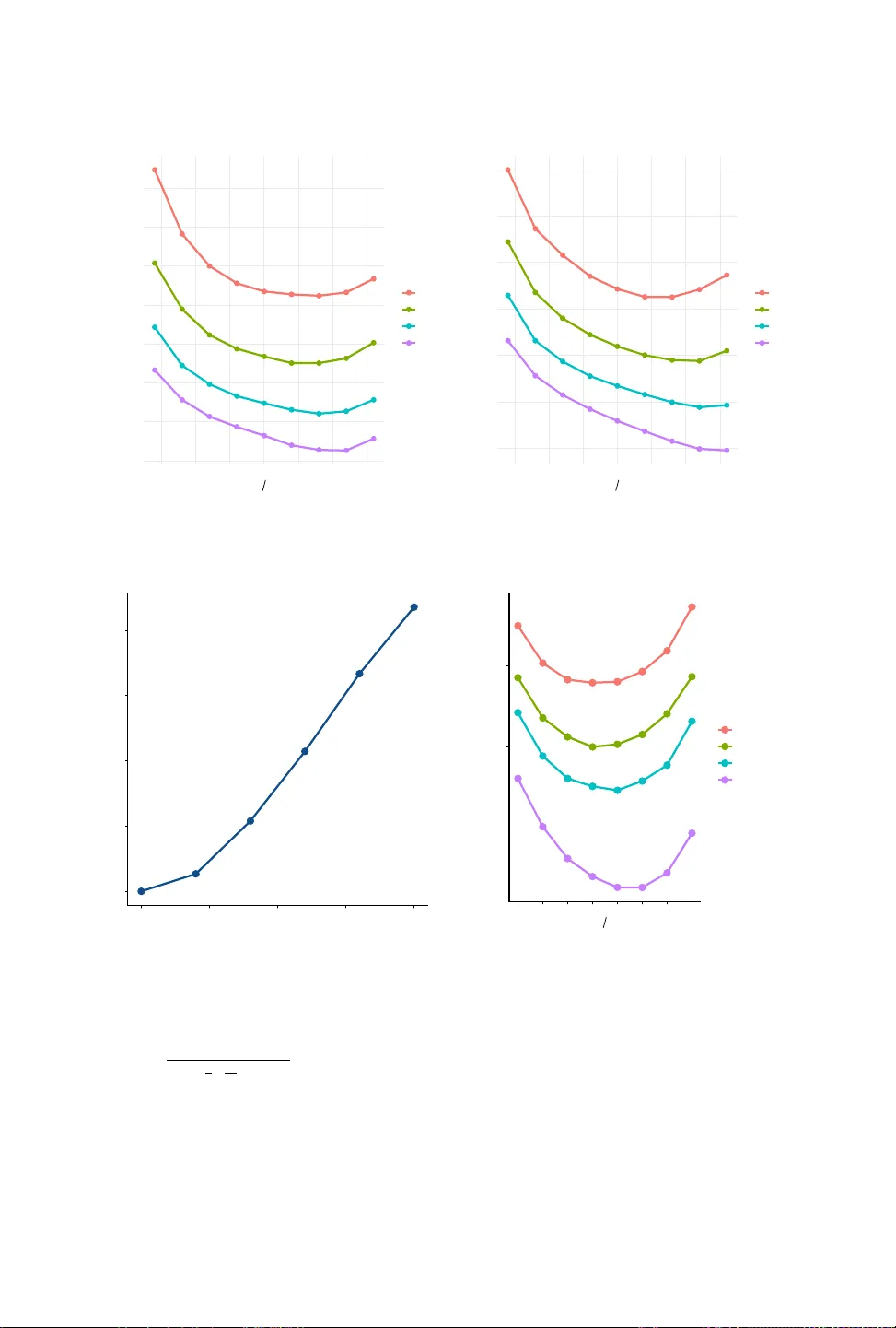
Dierential Privacy for Network Connectedness Indices TOM A. RU T TER, Y UXIN LIU, M. AMIN RAHIMIAN Researchers increasingly use data on social and economic networks to study a range of social science questions, but releasing statistics derived from networks can raise signicant privacy concerns. W e show how to release network connectedness indices that quantify assortative mixing across node attributes under edge-adjacent dierential privacy . Standard privacy techniques perform poorly in this setting both b ecause connectedness indices have high global sensitivity and because a single node’s attribute can potentially be an input to connectedness in thousands of cells, leading to poor composition. Our method, which is straightfor ward to apply , rst adds noise to node attributes, then analytically debiases downstream statistics, and nally applies a second layer of noise to protect the presence or absence of individual edges. W e prove consistency and asymptotic normality of our estimators for both discrete and continuous labels and show our method works well in simulations and on real networks with as fe w as 200 nodes collected by so cial scientists. Additional K ey W ords and Phrases: dierential privacy , netw ork statistics, social networks, connectedness indices, privacy–utility tradeo Contents 1 Introduction 1 2 Literature Review 3 3 Privacy and Connectedness Indices 4 3.1 A Composition Theorem for Implementing Edge- Adjacent Dierential Privacy 8 4 Dierential Privacy for Binary Labels: High and Low Status Connectedness 8 4.1 Consistency of Debiased Private Estimation for Network Connectedness 9 5 Dierential Privacy for Continuous Labels: Regressing Friends Rank on Own Rank 12 6 Accuracy on Simulated Networks 16 6.1 Binary Labels on Erdős-Rényi and Stochastic Blo ck Models 16 6.2 Continuous Labels on Graphons 17 7 Empirical Applications 18 7.1 Diusion Networks in Rural India 18 7.2 Mutual Follows on T witch 22 8 Discussion 22 A Proofs 26 A.1 Proof of Theorem 1: ( 𝜀, 𝛿 ) composition under edge-adjacency 26 A.2 Proof of Proposition 1: MVUE for individual conne ctedness 26 A.3 Proof of Theorem 2: Consistency of the debiased private estimator 27 A.4 Proof of Theorem 3: Edge- Adjacent DP Guarantee for Binar y Labels 30 A.5 Proof of Theorem 4: Asymptotic normality and perturbation order 31 A.6 Proof of Proposition 2: Consistency of Private Regression Estimators 38 A.7 Proof of Theorem 5: Edge- Adjacent DP Guarantee for Regression Estimates 42 A.8 Proof of Theorem 6: Asymptotic normality of the private debiased regression estimator 43 B Additional Material 46 B.1 Products frequently purchased together on Amazon 46 B.2 List of Notation 50 Rutter: Stanford University Department of Economics; Liu, Rahimian: University of Pittsburgh Swanson School of Engineering. Correspondence to: rahimian@pitt.edu. W e are grateful to Jordan A wan, Sahana Subramanyam, Sam Thau, three anonymous reviewers, participants at Theor y and Practice of Dierential Privacy 2025, the 2025 Google Research Conference on Ads Privacy , the Pitt Department of Statistics Seminar , and the Privacy and Public Policy Conference for helpful comments. Rutter acknowledges funding from the Knight- Hennessy scholarship. Code to replicate all of our analyses is available at: https://github.com/T omRutter42/Privacy-for-Connectedness-Indices. T om A. Rutter , Yuxin Liu, M. Amin Rahimian 1 1 Introduction Social scientists interested in a range of so cial phenomena are increasingly using data on the networks in which individuals, rms, nancial institutions and nations are embedded. (See, for example, Easley and J. Kleinberg (2010), Jackson (2019), and Goyal (2023) for overviews.) The use of network data has pr ovided valuable insights on the spread of contagious diseases, the r ole of peers and mentors in shaping people’s life outcomes, the resilience of global supply chains, and the nature of systemic risk in the nancial system. The use of such data, however , comes with concerns about the privacy protections provided to individuals and organizations in the dataset. The naive publication of aggregated statistics fr om these datasets entails risks that information may be leaked about the presence ( or lack thereof ) of particular connections in the dataset, or even ab out the individual characteristics of people or businesses represented in the data. In response to broader concerns about guaranteeing privacy for individuals and organizations represented in datasets used by so cial scientists, the literature on dierential privacy , starting from Dwork et al. (2006), has de velope d tools for allowing particular statistics to b e released from datasets while simultaneously providing a mathematical guarantee that, without making any assumptions on the external knowledge some one might have, it is imp ossible for anyone to learn too much about a given individual or organization in the data just from seeing the aggregated statistic. This literature was inspired by the failure of traditional data pr otection techniques, such as the removal of personally identiable information from datasets, to provide adequate protection to individuals whose records are contained in the data. For example, Narayanan and Shmatikov (2008) were able to cross-reference anonymized Netix movie ratings with public IMDB proles to identify specic users in the Netix database, despite the fact that the Netix movie ratings dataset did not in itself contain any personally identiable information. Even aggregated datasets can r eveal surprising amounts of information about particular individuals in the dataset if only naive data protection techniques, such as masking small cells or swapping some individuals between cells, are use d. For example, Dick et al. (2023) pr ovide reconstruction attacks on the 2010 US Census that allow them to reliably learn the characteristics of many individuals from the aggr egated data alone. The reason their attack works is that the Census released many tables containing aggregate statistics, so dierencing the statistics in particular tables (which aggr egate over dierent, but not mutually e xclusive, sets of individuals) allows them to hone in on the data for particular individuals. The increasing availability of compute power and access to articial intelligence will dramatically reduce the cost of carrying out futur e attacks on public data as well as the mathematical expertise required to execute them successfully . The key idea in the dierential privacy literature, which provides a mathematical guarantee that no possible attack can reveal much information about any one data point in the dataset, is to infuse random statistical noise into the aggregated statistic so that an outsider is not able to separate the inuence of a given individual on a statistic versus the inuence of the random noise. T ypically this noise is applie d on the basis of the sensitivity of the statistic to a change in any particular observation in the dataset. In the case of the Census reconstruction attack, the statistical noise introduced completely defeats the logic that dier encing dierent releases allows an attacker to get at the information of a particular individual in the dataset. For statistics constructed from networks, it can often be the case that the sensitivity of the statistic covers the entir ety of the parameter space, limiting the delity of the privatized statistic to its true value while maintaining a particular privacy guarantee. Inde ed, we show that this is the case for the class of network statistics we consider in this paper , so an alternative approach is required. T om A. Rutter , Yuxin Liu, M. Amin Rahimian 2 In this paper , we provide an approach for releasing a particular class of network statistics with a formal privacy guarantee that maintains high accuracy even for relatively small realistic networks. The statistics we consider are network conne ctedness indices , which describ e the proportion of connections from nodes with a given characteristic that extend to nodes with either the same characteristic or a dierent characteristic. For example, what pr op ortion of the friends of white individuals are also white? What proportion of the suppliers of US rms are based in China? What proportion of bank loans are directed to hedge funds? The application we focus on, which motivated this paper , concerns the proportion of friendships that cut across the income distribution. In a widely cited pair of studies, Chetty et al. (2022a) and Chetty et al. (2022b) publicly released a range of social capital indices constructed from Facebook and Instagram data for counties, zip codes, universities, and schools in the US. In particular , Chetty et al. (2022a) released a measure of the fraction of high-socio economic status (SES) friends among low-SES individuals in an area, which they single out as the strongest predictor of economic mobility in the US. (They use data fr om Chetty et al. (2026) and dene the e conomic mobility of an area as the average adult income rank of a child born to parents at the 25th percentile of the national income distribution.) The statistics they publicly released have been widely downloaded and used in follo w-on r esearch. Although the authors of these studies used tools from the dierential privacy literature to reduce the risk of privacy loss, the y did not provide a formal privacy guarantee for the connectedness indices they released. Subsequent work by Harris et al. (2025) extended these measures to the United Kingdom, and while they also infused noise into the data b efore making it public, they similarly did not provide a formal privacy guarantee. In this paper , we provide a simple-to-use method for publicly releasing network connectedness indices, such as economic connectedness, with a formal privacy guarantee. In practice, our methods allow for releasing conne ctedness indices constructed from realistic netw orks of at least 200 individuals with low levels of statistical noise . The ke y logic behind our approach is to rst inject random noise into the characteristics of nodes in the data, such that downstream statistics ar e calculated from a database of node characteristics that already satises a privacy guarantee. This is crucial in allowing us to sidestep consideration of the sensitivity of our statistics of interest to a change in node characteristics in “worst-case ” networks, such as star netw orks, which do not occur in practice. It also allows us to sidestep the issue that a change in the attribute of a node can potentially aect connectedness in a large number of cells, leading to po or composition. Instead, by privatizing no de characteristics and then assuming that all downstream statistics are computed from these sanitize d node-level data, we only have to consider the sensitivity of our statistics to changes in the e dge set, for which we show the sensitivity is much lower . Additionally , a particular edge (or lack ther eof ) can only change the value of connectedness in at most two cells, leading to much better composition. Injecting random noise into the node characteristics will often bias the downstream statistics, so we provide formulae for analytic corr e ctions that can also be applied downstream to debias these statistics while maintaining their privacy guarantees by the postprocessing theorem (Dwork and Roth, 2014, Proposition 2.1). W e note, crucially , that the database of individual characteristics is usually not of interest and so do es not have to b e (and usually should not b e) released. Although not releasing this intermediate dataset do es not reduce the mathematical privacy loss from data release, since we make no assumptions about the background knowledge of outsiders, in practice it provides an additional layer of privacy protection, since realistic outsiders do not have the extreme level of information that usually constitutes the worst case for a researcher trying to provide a privacy guarantee (Bassily et al., 2013). T om A. Rutter , Yuxin Liu, M. Amin Rahimian 3 Our paper procee ds as follows. Section 2 provides an overview of relevant literature on dierential privacy and the network statistics we consider . Section 3 outlines the denitions of privacy we use and network connectedness indices. Section 4 presents our method for binary labels. Se ction 5 extends our framework to continuous lab els. Section 6 presents simulations that evaluate the accuracy of our methods. Section 7 demonstrates the empirical performance of our methods on real-world labeled networks, and section 8 concludes. 2 Literature Review Our paper builds on the vast literature on dierential privacy that began with D work et al. (2006). Standard dierential privacy mechanisms tend to make use of the indep endence between records, but with network data records are clearly not indep endent (Kifer and Machanavajjhala, 2011). This dependence is not just a theoretical curiosity , but is a vulnerability that can be exploited in practice , as demonstrated by Liu et al. (2016) who infer sensitive location data for users from statistics that have a dierential privacy guarantee under independence. The above work highlights the need for privacy applications that explicitly account for statistical dependence in the data, as our method does for network connectedness indices. Our main contribution is to the practice of economic data release, and so our work builds on Chetty et al. (2022a) and Chetty et al. (2022b) who developed the notion of economic connectedness and released these statistics for granular US geographies, schools, and universities. The central innovation in those papers is showing that measures of network connecte dness constructed by combining information about who is connected to whom with information about the characteristics of the connected individuals can signicantly outperform measures based only on the edge structure of the network (such as the clustering coecient) or measures based only on node characteristics that ignore the connections between nodes (such as variables related to a neighborhood’s income composition) in explaining variation in economic outcomes such as intergenerational mobility . This insight that both the structure of the connections and the characteristics of connected individuals matter directly informs the notion of edge-adjacent privacy we use from Blocki et al. (2013), and allows us to pro vide a guarantee that we protect both the presence (or absence) of edges and the characteristics of nodes. Our pap er also relates to a literature on dierential privacy for dep endent data. Dependent dierential privacy and its generalizations address pairwise and arbitrary correlations, though they often rely on dependence parameters that are dicult to estimate without explicit probabilistic models (Liu et al., 2016; Zhao et al., 2017). A more exible alternativ e is the Puersh framework (Kifer and Machanavajjhala, 2014), which allows for customized privacy denitions—such as Blowsh and Bayesian DP—by explicitly modeling secrets, discriminative pairs, and data generation distributions. In the context of graph data, Puersh implementations like the W asserstein and Markov quilt mechanisms have demonstrated superior utility over group DP by leveraging Bayesian networks to model dependencies (Song et al., 2017). Complementary approaches include inferential privacy , which uses Markov chains to quantify correlation (Ghosh and R. Kleinberg, 2016), and zero-knowledge privacy , which pro vides stronger guarante es for spe cic graph properties like connectivity (Gehrke et al., 2011). Especially in graph settings, a common approach is to project onto a graph with a low maximum degree, to decrease the sensitivity of statistics (Kasiviswanathan et al., 2013). In many settings this technique works very well, but for the applications we ar e interested in, degree heterogeneity is an important feature of the data that can be lost when projecting onto a graph with a low maximum degree. (For example, Harris et al. (2025) show that degree variation by SES in the UK is an important feature of netw orks when considering connectedness indices—imposing a low degr ee bound in this T om A. Rutter , Yuxin Liu, M. Amin Rahimian 4 particular setting could dramatically change estimates of connectedness.) See Hehir et al. (2025) for a review of various notions of dier ential privacy for networks and their interpretation. 3 Privacy and Connectedness Indices W e follow Dwork et al. (2006) and the dierential privacy literature in adopting a denition of privacy that requires the pr obability that any statistical output b eing produced from two close datasets to be similar . Definition 1 ( 𝜀 -differential priv acy). A randomized mechanism M is 𝜀 -dierentially private if for all adjacent datasets 𝐷 and 𝐷 ′ and all possible sets S of outputs of the mechanism we have:     ln  P ( M ( 𝐷 ) ∈ S ) P ( M ( 𝐷 ′ ) ∈ S )      ≤ 𝜀 An intuitive interpretation of this denition is that an adversary with unrestricted information about the rest of the dataset cannot be come much more condent that the true dataset is 𝐷 as opposed to 𝐷 ′ , or vice versa, after observing the output of M . Our goal in this paper is to construct a mechanism that outputs estimates of connectedness indices that satisfy 𝜀 -dierential privacy . T o x notation, we rst dene a labele d network. Definition 2 (Labeled Network). A lab eled network is a triple ( V , E , L ) , where V is the set of vertices, E is the set of edges, and L = ( 𝑙 𝑖 ) 𝑖 ∈ V , 𝑙 𝑖 ∈ { 𝑎, 𝑏 } , is the node label vector that assigns each node a label from the set of labels { 𝑎, 𝑏 } . Note that this denition is analogous to the denition of a social network in Blocki et al. (2013). A pair of possible labels for a node could be, for example, “high SES” or “low SES” . For notation we dene 𝑒 𝑖 𝑗 = 1 if ( 𝑖 , 𝑗 ) ∈ E (that is, if there is an e dge between 𝑖 and 𝑗 ) and 𝑒 𝑖 𝑗 = 0 otherwise. W e denote node 𝑖 ’s degree as: 𝑑 𝑖 =  𝑗 ∈ V 𝑒 𝑖 𝑗 and the neighborhood of no de 𝑖 as the set of nodes 𝑖 is connected to: 𝑁 ( 𝑖 ) = { 𝑗 ∈ V : 𝑒 𝑖 𝑗 = 1 } Definition 3 (Cross-Type Connectedness Index). T ake a lab eled network ( V , E , L ) , where L = ( 𝑙 𝑖 ) 𝑖 ∈ V , 𝑙 𝑖 ∈ { 𝑎, 𝑏 } . Dene the induced partition of nodes by A : = { 𝑖 ∈ V : 𝑙 𝑖 = 𝑎 } , B : = { 𝑖 ∈ V : 𝑙 𝑖 = 𝑏 } . The cross-type conne ctedness index from A to B is dened as 𝐶 A → B : = 1 # ( A )  𝑖 ∈ A Í 𝑗 ∈ B 𝑒 𝑖 𝑗 𝑑 𝑖 . T om A. Rutter , Yuxin Liu, M. Amin Rahimian 5 Set A Set B A1 A2 B1 B2 Node A1 Friends in B : 2 (B1, B2) T otal Friends: 3 (A2, B1, B2) 𝜌 𝐴 1 = 2 3 Node A2 Friends in B : 1 (B2) T otal Friends: 2 (A1, B2) 𝜌 𝐴 2 = 1 2 𝐶 A → B = 2 3 + 1 2 2 = 7 12 Fig. 1. An example of how to calculate the cross-type connectedness index. That is, 𝐶 A → B is the average fraction of connections from individuals in group A to individuals in group B . Chetty et al. (2022a) and Chetty et al. (2022b) produce thr ee dierent types of cross-type con- nectedness index for US counties, zip codes, schools, and universities in the US: (1) economic connectedness (the average fraction of high-SES friends among low-SES individ- uals). (2) language connectedness (the average fraction of friends who use English as their primary language among individuals who do not use English as their primary language). (3) age connectedness (the av erage fraction of friends age 35–44 among individuals age 25–34). Bailey et al. (2025) pr o duce a cross-type connectedness index measuring the average fraction of female friends among male individuals. For notation, we let: 𝜌 𝑖 : = Í 𝑗 ∈ B 𝑒 𝑖 𝑗 𝑑 𝑖 from here on, so that a cross-type connectedness index can be written: 𝐶 A → B = 1 # ( A )  𝑖 ∈ A 𝜌 𝑖 W e pro vide a simple example illustrating the cross-type connectedness inde x in Figure 1. In T able 1, we provide a summar y of our notation. (W e provide a mor e extensive list of our notation in T able B.2.) W e can also dene a same-type connectedness index , which is the proportion of conne ctions extending from one group of nodes to themselves. T om A. Rutter , Yuxin Liu, M. Amin Rahimian 6 T able 1. Summary of Notation Symbol Description V Set of vertices (nodes) in the network E Set of edges (friendships/connections) between no des L = ( 𝑙 𝑖 ) 𝑖 ∈ V Node label vector with 𝑙 𝑖 ∈ { 𝑎, 𝑏 } for each node 𝑖 𝑒 𝑖 𝑗 Binary indicator; 𝑒 𝑖 𝑗 = 1 if an e dge exists between 𝑖 and 𝑗 , else 0 𝑑 𝑖 Degree of node 𝑖 , # ( 𝑗 ∈ V : 𝑒 𝑖 𝑗 = 1 ) . 𝑁 ( 𝑖 ) Neighborhood of no de 𝑖 , { 𝑗 ∈ V : 𝑒 𝑖 𝑗 = 1 } . A , B Partitions of V base d on labels ( 𝑎, 𝑏 ) # ( ·) Cardinality operator (number of elements in a set) 𝜌 𝑖 Individual 𝑖 ’s fraction of friends belonging to the target group 𝐶 A → B Cross-type connectedness index (average 𝜌 𝑖 for individuals in group A ) Definition 4 (Same-Type Connectedness Index). T ake a labeled network ( V , E , L ) , where L = ( 𝑙 𝑖 ) 𝑖 ∈ V , 𝑙 𝑖 ∈ { 𝑎, 𝑏 } . Dene the induced partition of nodes by A : = { 𝑖 ∈ V : 𝑙 𝑖 = 𝑎 } , B : = { 𝑖 ∈ V : 𝑙 𝑖 = 𝑏 } . The same-typ e connectedness index for group A is dened as 𝐶 A → A : = 1 # ( A )  𝑖 ∈ A Í 𝑗 ∈ A 𝑒 𝑖 𝑗 𝑑 𝑖 . That is, 𝐶 A → A is the average fraction of connections from individuals in A to other individuals in the same group A . Note that 𝐶 A → A = 1 − 𝐶 A → B . W e often will want to compute cross-type connectedness indices for a particular cell , wher e a cell could be, for example, a county , a zip code, or a school. In that case , if we let 𝑠 denote the cell ( a set of users, such as a school) we can consider the statistics: 𝐶 A → B 𝑠 = 1 # ( A ∩ 𝑠 )  𝑖 ∈ A ∩ 𝑠 Í 𝑗 ∈ B 𝑒 𝑖 𝑗 𝑑 𝑖 or: 𝐶 A → B 𝑠 = 1 # ( A ∩ 𝑠 )  𝑖 ∈ A ∩ 𝑠 Í 𝑗 ∈ B ∩ 𝑠 𝑒 𝑖 𝑗 Í 𝑗 ∈ V ∩ 𝑠 𝑒 𝑖 𝑗 with the dierence being whether we consider only friendships from individuals in the cell to other individuals in the cell, or whether we consider connections from individuals in the cell to any other individual. For our privacy guarantee, w e will follo w the notion of edge-adjacent DP from Blocki et al. (2013), which allows us to protect both the characteristics of individual nodes in the netw ork (such as an individual’s income or race) and the presence or absence of particular edges in the network. This is 𝜀 -DP when considering labeled networks as adjacent if they satisfy the following property: T om A. Rutter , Yuxin Liu, M. Amin Rahimian 7 R R R R R R R B R R R R R R Change the label of the central node Network G Every Red node has zero Blue friends. Red-to-Blue Connectedness = 0 Network G’ Every Red node has only Blue friends. Red-to-Blue Connectedness = 1 Fig. 2. A star-network illustration of why node-level privacy notions can be to o strong for connectedness statistics: modifying the center node (or pr otecting its presence/incident edges under node-DP) can move red-to-blue connectedness from 0 to 1 , implying sensitivity that spans [ 0 , 1 ] and does not diminish with network size. Definition 5 (Edge-Adjacent Labeled Networks). T wo labeled networks ( V , E , L ) and ( V , E ′ , L ′ ) are said to be e dge-adjacent if: • the edge sets E and E ′ dier by at most one edge, and • the label vectors L = ( 𝑙 𝑖 ) 𝑖 ∈ V and L ′ = ( 𝑙 ′ 𝑖 ) 𝑖 ∈ V dier in at most one component, i.e., there exists at most one node 𝑢 ∈ V such that 𝑙 𝑢 ≠ 𝑙 ′ 𝑢 . That is, two netw orks are edge adjacent if they dier in the presence of at most one edge and the characteristic of at most one node. The name edge-adjacent is somewhat unfortunate since it does allow for node characteristics to vary , but we stick with this terminology for consistency with the prior literature. The notion of edge-adjacent DP has been employed by Jorgensen et al. (2016) and Chen et al. (2020). W e note that our notion of edge-adjacency is slightly stronger than that stated by Blo cki et al. (2013), since we allow for a simultaneous change in b oth an edge and the characteristics of one node, as opposed to a change in either an edge or the characteristics of one node. Note that our adjacency notion does not treat the presence of a node in the dataset as private. Requiring node pr esence privacy would move us towar d node-level DP (node-DP), under which two graphs are adjacent if one can be obtained from the other by adding/removing a vertex together with (potentially) all incident edges. In social network settings, this stronger notion is typically infeasible for connectedness statistics: the removal of a single high-degree vertex can drastically change cross-type connectivity , forcing any DP mechanism to inject noise at a scale that overwhelms the signal. Figure 2 provides a simple illustration: changing the center node (or equivalently , protecting its presence/incident edges under node-DP) can shift the red-to-blue connectedness from 0 to 1 , so the sensitivity spans the entire parameter space and does not diminish with network size. Accordingly , we follow the modeling p erspective advocated by Chen et al. (2020): on many platforms the existence of user proles (and hence the verte x set V ) is eectively public, whereas T om A. Rutter , Yuxin Liu, M. Amin Rahimian 8 personal characteristics recorded on proles are sensitive . Our goal is therefore to protect node attributes and individual edges ( via edge-adjacent DP), rather than node presence, which would render the connectedness indices of interest non-actionable. 3.1 A Composition Theorem for Implementing Edge- Adjacent Dierential Privacy In this section, we provide a method that allows the release of conne ctedness indices with a formal privacy guarantee. The core logic behind our approach is as follows. A connectedness index risks releasing informa- tion about two characteristics of a giv en node in the netw ork— the no de ’s label and its friendships— and this is reected in the notion of edge-adjacent DP w e use. The approach used by Chetty et al. (2022a) and Chetty et al. (2022b) to protect economic connectedness involves computing the economic connectedness metric and then applying noise to the aggregated statistic on the basis of its local sensitivity to changes in the node’s characteristic and friendships. 1 W e show that applying noise to the node characteristics and then adjusting for the bias this creates in the ensuing estimate of economic connectedness, followed by applying noise on the basis of sensitivity to changes in a no de ’s friendship network, is a better approach that allows for a formal privacy guarantee while injecting small amounts of noise. 2 Our approach rests on the following theorem (prov e d in Section A.1), which formalizes the composition principle underlying this construction. It states that applying a private me chanism to node attributes, and then a separate edge-DP mechanism for the aggregate statistic that takes as an input the privatized attributes, composes in a way that satises edge-adjacent DP. Theorem 1 ( ( 𝜀 , 𝛿 ) composition under edge-adja cency). Let ( V , E , L ) and ( V , E ′ , L ′ ) be edge- adjacent labeled networks. Let M 1 : ( V , E , L ) ↦→ ( V , E , b L ) be ( 𝜀 ℓ , 𝛿 ℓ ) -DP with respect to changing a single node attribute, and for every xed b L let M 2 ( · , b L ) : ( V , E ) ↦→ R be ( 𝜀 𝑒 , 𝛿 𝑒 ) -DP with respect to changing a single e dge. Dene the composed mechanism M : = M 2 ◦ M 1 . Then M is ( 𝜀 ℓ + 𝜀 𝑒 , 𝛿 ℓ + 𝑒 𝜀 ℓ 𝛿 𝑒 ) edge-adjacent dierentially private. 4 Dierential Privacy for Binary Labels: High and Low Status Connectedness W e now make use of the general composition frame work establishe d in The orem 1. In particular , we rst construct an 𝜀 ℓ -DP mechanism M 1 for node attributes, and subse quently apply an 𝜀 𝑒 edge-DP mechanism to the aggregate statistic computed from the privatized labels. Our rst step is therefore to protect node attributes under 𝜀 𝑙 -DP using randomized response. Specically , for each node 𝑖 , the categorical lab el 𝑙 𝑖 ∈ { 𝑎, 𝑏 } is independently randomized by ipping its value with probability 𝑝 = 1 1 + 𝑒 𝜀 𝑙 , yielding a private label ˆ 𝑙 𝑖 . 1 The notion of local sensitivity is from Nissim et al. (2007). Howev er , while the smooth sensitivity approach developed by Nissim et al. (2007) is formally private , the local-sensitivity-base d method used by Chetty et al. (2022a) and Chetty et al. (2022b), which leverages the maximum observed sensitivity approach of Chetty and Friedman (2019), is not formally private because the maximum observed sensitivity itself is a function of the private data and so can leak information about outliers. 2 It also sidesteps a key diculty that would otherwise be emb edded in this problem, which is that the label of a given node is potentially an input to the conne ctedness index for every single cell in the dataset (since a node can potentially b e connected to a node in every other cell). This causes composition issues for approaches based on the global sensitivity of change to a node’s label, since privacy losses compose in the product of the number of cells and number of statistics released. Our approach only composes in the number of statistics released. This is because once the node labels are privatized, by the postprocessing theorem, any number of subse quent cell-level indices can be derived from these private labels without further depleting the privacy budget reserved for node characteristics. T om A. Rutter , Yuxin Liu, M. Amin Rahimian 9 Fact 1. Let each no de ’s attribute be 𝑙 𝑣 ∈ { 𝑎, 𝑏 } , and let L = ( 𝑙 𝑣 ) 𝑣 ∈ V denote the label vector . Dene the randomized mechanism M 1 that independently replaces each node’s attribute according to M 1 ( 𝑙 𝑣 ) =            𝑙 𝑣 , with probability 1 − 𝑝 = 𝑒 𝜀 𝑙 1 + 𝑒 𝜀 𝑙 the opposite value in { 𝑎, 𝑏 } , with probability 𝑝 = 1 1 + 𝑒 𝜀 𝑙 Then M 1 satises 𝜀 𝑙 -dierential privacy with respect to changes in a single no de ’s attribute. Proof. This property of randomize d response is well known in the DP literature. See, for example, Result 1 of W ang et al. (2016) for a proof of this property . □ One potential issue with this approach is that randomized response induces attenuation bias in the connectedness metric. When using an above- vs below-median split, randomly ipping node labels mechanically pushes observed group composition toward 1 / 2 , even when true homophily is strong. For example, if 𝑝 = 1 2 , then regardless of the true level of homophily in society , in expectation half of every node’s neighbors will appear to belong to group 𝑏 under the privatized labels. W e therefore require a correction mechanism that recovers unbiased estimates of cross-type connectedness using only the privatized labels ˆ 𝑙 𝑖 , without accessing the nonprivate lab els 𝑙 𝑖 . Propo- sition 1 (prov e d in Section A.2) constructs a minimum-variance unbiased estimator (MVUE) that corrects for this attenuation bias using only the randomized-response outputs. Proposition 1 (MVUE for individu al connectedness). For each node 𝑖 , dene the true indi- vidual connectedness 𝜌 𝑖 : =  𝑗 ∈ V 𝑎 𝑖 𝑗 1 { 𝑙 𝑗 = 𝑏 } , 𝑎 𝑖 𝑗 : = 𝑒 𝑖 𝑗 𝑑 𝑖 . Let privatized labels ˆ 𝑙 𝑗 be generated by randomized response with ipping probability 𝑝 = 1 1 + 𝑒 𝜀 𝑙 , and dene the observed proxy ˆ 𝜌 𝑖 : =  𝑗 ∈ V 𝑎 𝑖 𝑗 1 { ˆ 𝑙 𝑗 = 𝑏 } . Then the unique minimum-variance unbiased estimator (MV UE) of 𝜌 𝑖 based only on the privatize d labels ( ˆ 𝑙 𝑗 ) 𝑗 ∈ 𝑉 is ˜ 𝜌 𝑖 : = ˆ 𝜌 𝑖 − 𝑝 1 − 2 𝑝 . (1) 4.1 Consistency of Debiased Private Estimation for Network Connectedness Proposition 1 establishes that ˜ 𝜌 𝑖 is unbiased (indeed MV UE) for the individual connectedness 𝜌 𝑖 given the privatized labels. However , our target estimand is a cell-level connectedness index , which aggregates 𝜌 𝑖 over a latent subset of nodes (e .g., 𝐴 ∩ 𝑠 ) and is implemented via a ratio (a Hájek-type normalization). Unbiasedness of the individual components does not automatically imply that the resulting ratio estimator is unbiased or w ell-behaved in nite samples, and in particular it does not control the probability that the random denominator is close to zero . Moreover , the nal released statistic additionally includes edge-DP noise calibrated to an edge-sensitivity that shrinks with the population size. T om A. Rutter , Yuxin Liu, M. Amin Rahimian 10 Dene the debiased weight for membership in A : 𝑤 𝑖 : = 1 { b 𝑙 𝑖 = 𝑎 } − 𝑝 1 − 2 𝑝 . (2) Let 𝑆 0 , 𝑛 : =  𝑖 ∈ 𝑉 𝑤 𝑖 , 𝑆 1 , 𝑛 : =  𝑖 ∈ 𝑉 𝑤 𝑖 ˜ 𝜌 𝑖 , where ˜ 𝜌 𝑖 is the debiased proxy for 𝜌 𝑖 in Eq. (1). The Hájek-type estimator is e 𝐶 A → B : = 𝑆 1 , 𝑛 𝑆 0 , 𝑛 , (3) whenever 𝑆 0 , 𝑛 ≠ 0 (we sho w that 𝑆 0 , 𝑛 is bounded away from 0 with probability tending to 1 under mild conditions). W e ne xt establish a large-sample guarantee: under mild r egularity conditions, the debiased Hájek estimator is consistent , and the additional e dge-DP noise is asymptotically negligible, so the overall private r elease conv erges in probability to the true connectedness index. T o state the result, w e rst introduce two regularity conditions. The rst ensur es that the target cell remains asymptotically non-negligible, so that the random denominator in the Hájek normalization does not go to zero . The second is a b ounded-degree condition, which controls local dependence and ensures that b oth the estimator and its edge-sensitivity remain uniformly well behaved. Assumption 1 (Non-v anishing fraction of type- 𝐴 nodes). There exists 𝜋 A ∈ ( 0 , 1 ] such that # ( A ) / 𝑛 → 𝜋 A as 𝑛 → ∞ . Assumption 2 (Bounded degree). There exists Δ < ∞ such that for all 𝑛 and all 𝑖 ∈ 𝑉 , 𝑑 𝑖 ≤ Δ . (4) In order to implement the second stage of the construction in Se ction 3.1, we must calibrate the edge-DP noise added to the aggregate statistic. Since the Laplace mechanism r equires an upper bound on the e dge-sensitivity of the released quantity , we therefore compute the sensitivity of 𝑆 1 , 𝑛 to the addition or removal of a single edge. Importantly , at this stage the privatized labels b L have already been generate d via M 1 . Hence, ( 𝑤 𝑖 ) 𝑖 ∈ 𝑉 , 𝑆 0 , and the debiasing factors are all xed, and we only need to control how 𝑆 1 , 𝑛 changes when the edge set varies. The following lemma establishes a uniform bound on this edge-sensitivity (proved in Section A.3, along with other auxiliary lemmas for consistency of the private network connectedness estimator). Lemma 1 (Edge-sensitivity of 𝑆 1 , 𝑛 ). Fix ( ˆ 𝑙 𝑖 ) 𝑖 ∈ 𝑉 , so that ( 𝑤 𝑖 ) 𝑖 ∈ 𝑉 is xed. Let 𝐸 and 𝐸 ′ dier by the addition or removal of a single e dge ( 𝑢, 𝑣 ) . Assume ˆ 𝜌 𝑖 ( 𝐸 ) is computed ro w-wise as ˆ 𝜌 𝑖 ( 𝐸 ) = Í 𝑗 𝑎 𝑖 𝑗 ( 𝐸 ) 1 { ˆ 𝑙 𝑗 = 𝑏 } with 𝑎 𝑖 𝑗 ( 𝐸 ) = 𝑒 𝑖 𝑗 / 𝑑 𝑖 (so only the normalized weight rows for 𝑢 and 𝑣 change when adding or removing ( 𝑢 , 𝑣 ) ). Then,   𝑆 1 , 𝑛 ( 𝐸 ) − 𝑆 1 , 𝑛 ( 𝐸 ′ )   ≤ 2 ( 1 − 𝑝 ) ( 1 − 2 𝑝 ) 2 . W e next study the asymptotic behavior of the propose d estimator . Although e 𝐶 A → B is constructed from unbiased components, it is a ratio estimator and the nal r elease additionally includes edge-DP noise. It is therefor e not immediate that the private estimator remains well behaved as 𝑛 gro ws. The following theorem establishes consistency and shows that the added edge-DP noise is asymptotically negligible (proved in Section A.3). T om A. Rutter , Yuxin Liu, M. Amin Rahimian 11 Theorem 2 (Consistency of the debiased priv a te estima t or). Suppose Assumptions 1 and 2 hold, with 𝑝 ∈ ( 0 , 1 2 ) . Let e 𝐶 A → B = 𝑆 1 , 𝑛 / 𝑆 0 , 𝑛 be the debiased Hájek-type estimator in (3) . Dene the edge-DP release b 𝐶 A → B DP : = e 𝐶 A → B + 𝑍 𝑛 , 𝑍 𝑛 ∼ Lap  0 , 2 ( 1 − 𝑝 ) ( 1 − 2 𝑝 ) 2 𝜀 𝑒 𝑆 0 , 𝑛  , where 𝑍 𝑛 is independent of the randomized-response perturbations. Then, for any xed 𝜀 𝑒 > 0 , b 𝐶 A → B DP 𝑝 − → 𝐶 A → B , as 𝑛 → ∞ . W e summarize our approach in Algorithm 1. Algorithm 1 Dierentially Private Cross- T yp e Connectedness Index Require: Network ( V , E ) (with weights 𝑒 𝑖 𝑗 ≥ 0 ), node labels 𝑙 𝑖 ∈ { 𝑎, 𝑏 } , privacy parameter 𝜀 𝑙 , 𝜀 𝑒 . Ensure: Dierentially private connectedness index b 𝐶 A → B DP 1: 𝑝 ← 1 1 + 𝑒 𝜀 𝑙 2: for each no de 𝑖 ∈ V do ⊲ Randomized response on labels 3: ˆ 𝑙 𝑖 ← ( the opposite value in { 𝑎, 𝑏 } , with probability 𝑝, 𝑙 𝑖 , with probability 1 − 𝑝 4: end for 5: for each no de 𝑖 ∈ V do ⊲ Compute debiased weights and individual connectedness 6: ˆ 𝜌 𝑖 ←        1 𝑑 𝑖 Í 𝑗 ∈ 𝑁 ( 𝑖 ) 1 { ˆ 𝑙 𝑗 = 𝑏 } , 𝑑 𝑖 > 0 , 0 , 𝑑 𝑖 = 0 7: 𝑤 𝑖 ← 1 { ˆ 𝑙 𝑖 = 𝑎 } − 𝑝 1 − 2 𝑝 8: ˜ 𝜌 𝑖 ← ˆ 𝜌 𝑖 − 𝑝 1 − 2 𝑝 9: end for 10: 𝑆 0 , 𝑛 ← Í 𝑖 ∈ V 𝑤 𝑖 11: 𝑆 1 , 𝑛 ← Í 𝑖 ∈ V 𝑤 𝑖 ˜ 𝜌 𝑖 12: b 𝐶 A → B DP ← 𝑆 1 , 𝑛 𝑆 0 , 𝑛 + 𝑍 𝑛 , 𝑍 𝑛 ∼ Lap  0 , 2 ( 1 − 𝑝 ) ( 1 − 2 𝑝 ) 2 𝜀 𝑒 𝑆 0 , 𝑛  ⊲ Privatized Hájek estimator 13: return b 𝐶 A → B DP Based on Algorithm 1, we no w state the ov erall privacy guarantee of the proposed procedure. The result follows dir e ctly from Theorem 1, together with the 𝜀 ℓ -DP property of the randomized response and the 𝜀 𝑒 edge-DP calibration of the Laplace mechanism (proved in Section A.4). Theorem 3 (Priv acy gu arantee of Algorithm 1). Algorithm 1 satises ( 𝜀 ℓ + 𝜀 𝑒 ) edge-adjacent dierential privacy with respect to the input ( V , E , L ) . As established in Theorem 3, Algorithm 1 provides a clear decomposition of the overall privacy budget: the label-privatization step contributes 𝜀 ℓ , while the nal edge-private release contributes 𝜀 𝑒 . By sequential composition, the entire procedure therefore satises ( 𝜀 ℓ + 𝜀 𝑒 ) edge-adjacent dierential privacy . T om A. Rutter , Yuxin Liu, M. Amin Rahimian 12 Theorem 4 (Asympt otic normality and perturba tion order). Under the setup of Algorithm 1, suppose Assumptions 1–2 hold, the maximum degree is uniformly b ounded, and # ( A ) 𝑛 → 𝜋 A ∈ ( 0 , 1 ) . Let ˆ 𝜃 𝑛 : = 𝑆 1 , 𝑛 𝑆 0 , 𝑛 , 𝜃 𝑛 : = E [ 𝑆 1 , 𝑛 ] E [ 𝑆 0 , 𝑛 ] , and dene 𝑇 𝑛 : =  𝑆 0 , 𝑛 𝑆 1 , 𝑛  . Let the nal private release b e ˆ 𝜃 𝐷 𝑃 𝑛 : = ˆ 𝜃 𝑛 + 𝑍 𝑛 , where 𝑍 𝑛 | 𝑆 0 , 𝑛 ∼ Lap  0 , 2 ( 1 − 𝑝 ) ( 1 − 2 𝑝 ) 2 𝜀 𝑒 𝑆 0 , 𝑛  . Under Assumptions 1–2, it follows that 1 𝑛 Cov ( 𝑇 𝑛 ) → Σ for some nite matrix Σ , and that the asymptotic variance 𝜎 2 = ∇ 𝑔 ( 𝜇 0 , 𝜇 1 ) ⊤ Σ ∇ 𝑔 ( 𝜇 0 , 𝜇 1 ) is well dened, where 𝑔 ( 𝑥 , 𝑦 ) = 𝑦 / 𝑥 and ( 𝜇 0 , 𝜇 1 ) = lim 𝑛 →∞ E  𝑇 𝑛 𝑛  , 𝜇 0 > 0 . Then √ 𝑛 ( ˆ 𝜃 𝑛 − 𝜃 𝑛 ) ⇒ N ( 0 , 𝜎 2 ) . In addition, V ar ( 𝑍 𝑛 ) = Θ ( 𝑛 − 2 ) . Therefore , the additional edge-private Laplace perturbation is asymptotically negligible relative to the root- 𝑛 uctuation scale of the privatized ratio estimator . As established in Theorem 4, the dominant source of uncertainty comes from the label random- ization of ˆ 𝜃 𝑛 , rather than from the additional edge-private perturbation. Since the variance of the Laplace noise is of order 𝑛 − 2 , it does not aect the rst-order asymptotic distribution of the r eleased estimator . 5 Dierential Privacy for Continuous Labels: Regressing Friends Rank on Own Rank While our results so far have focused on network connectedness indices with binary labels, we expect that our method of applying noise directly to sensitive attributes and calculating statistics from private input vectors will b e helpful for a range of statistics relating to labeled networks. W e illustrate this with applications of our approach to statistics being developed for release in forthcoming pap ers that make use of continuous bounded labels for nodes in the network, as opposed to the discrete labels we considered before. Specically , these papers construct statistics relating to the average friend label among nodes with a giv en rank or among nodes falling within a given set of ranks. More generally , our techniques will be useful for providing dierentially private answers to questions such as whether less liquid rms tend to also rely on less liquid suppliers, T om A. Rutter , Yuxin Liu, M. Amin Rahimian 13 whether green rms tend to source materials from other gr een rms, or whether students display homophily on test scores. First, assign all individuals 𝑗 in the dataset a characteristic 𝑥 𝑗 in a connected and bounde d domain in R , without loss of generality we can take this domain to be [ 0 , 1 ] . 𝑥 𝑗 can, for example, be a continuous socioeconomic status indicator , as in the abov e papers, but more generally will often be a percentile rank on some numerical characteristic. For a set of users A we can consider the average friend rank of individuals in a set-cell combination. Let 𝑦 𝑖 denote the average friend rank of individual 𝑖 : 𝑦 𝑖 = Í 𝑗 ∈ 𝑁 ( 𝑖 ) 𝑥 𝑗 𝑑 𝑖 . Consider a regr ession of 𝑦 𝑖 on 𝑥 𝑖 , and let ˜ 𝛼 and ˜ 𝛽 denote estimates of the intercept and slope of this regression respectively . Definition 6 (Mean A verage Friend Rank). The mean average friend rank of individuals in a set A is: MAFR A 𝑠 = ˜ 𝛼 + ˜ 𝛽 ∫ A 𝑥 d 𝑥 ∫ A 1 d 𝑥 . (5) That is, we rst nd the average rank of friends for each individual 𝑖 ∈ A , and then take the average of this over all individuals in A . The term “mean average friend rank” captures the double average involved in Eq. (5); rst over friends of particular individuals, then over individuals in the relevant set). All of the statistics we consider in this section can be derived from the regression line where the 𝑥 variable is a node’s label and the 𝑦 variable is the average label of a node ’s conne ctions. By the postprocessing theorem, the problem then becomes to construct a dierentially private regression line. First, recall that only measurement err or (induced here by the dierential privacy pr ocedure) in the 𝑥 -variable biases a regr ession line, whereas zero-mean noise applied to the 𝑦 -variable will increase the standard errors associated with the regr ession output but not aect its expectation. T o correct for this bias, supp ose 𝑦 𝑖 = 𝛼 + 𝛽 𝑥 𝑖 + 𝜈 𝑖 , E [ 𝜈 𝑖 | 𝑥 𝑖 ] = 0 , and let ˆ 𝑦 𝑖 = 𝑦 𝑖 + 𝜂 𝑖 , ˆ 𝑥 𝑖 = 𝑥 𝑖 + 𝑢 𝑖 , where E [ 𝜂 𝑖 | 𝑦 𝑖 ] = 0 , E [ 𝑢 𝑖 | 𝑥 𝑖 ] = 0 , E [ 𝑢 2 𝑖 | 𝑥 𝑖 ] = 𝜎 2 . If 𝛽 ∗ denotes the slope coecient from the regression of ˆ 𝑦 on ˆ 𝑥 , then the standard errors-in-variables correction is ˜ 𝛽 = 𝛽 ∗  1 𝑛 − 1  Í 𝑖 ( ˆ 𝑥 𝑖 − ¯ ˆ 𝑥 ) 2  1 𝑛 − 1  Í 𝑖 ( ˆ 𝑥 𝑖 − ¯ ˆ 𝑥 ) 2 − 𝜎 2 (6) which is consistent for the true regression coecient 𝛽 . The corresponding intercept estimator is ˜ 𝛼 = ¯ 𝑦 − ˜ 𝛽 ¯ 𝑥 , which is consistent for 𝛼 . W e apply this correction to the privatized regression output below . For completeness, we state the result formally in Proposition 2 and provide a proof in Appendix A.6; see also Greene (2012) for related discussions. T om A. Rutter , Yuxin Liu, M. Amin Rahimian 14 W e now describe the privacy mechanism, which has two components. First, since 𝑥 𝑗 ∈ [ 0 , 1 ] , we privatize each individual characteristic by adding truncated Laplace noise, obtaining a privacy- protected rank ˆ 𝑥 𝑗 . Following Geng et al. (2020), this mechanism is calibrate d to the desired privacy level and keeps the perturbe d characteristic bounded, unlike the standard Laplace me chanism with unbounded support. This rst step protects the sensitive node lab els themselves. Second, w e compute the regression using the privatized covariates and the corresponding private friend-rank outcomes, and then apply Algorithm 3 to the resulting bounde d regr ession problem. The second step adds privacy protection at the regression stage; combine d with the rst-step perturbation of the node labels, this yields released r egression coecients that satisfy edge-adjacent dierential privacy . Applying bounded noise in the rst step is espe cially useful here, since the privacy guarantees for bounded linear regression require the co variates and outcomes to remain in a bounded range (Holohan et al., 2019), and the scale of the downstream noise added by Algorithm 3 depends on those bounds. From here, we can form an average friend rank for each individual 𝑖 that does not leak information about any of the 𝑥 𝑗 as: d AFR 𝑖 = Í 𝑗 ∈ 𝑁 ( 𝑖 ) ˆ 𝑥 𝑗 𝑑 𝑖 Note that these private friend ranks may also not lie between [ 0 , 1 ] since ˆ 𝑥 𝑗 may not lie between [ 0 , 1 ] . Howev er , since we apply noise from a bounde d domain, d AFR 𝑖 is still bounded, and so the sensitivity of the regression slope and intercept is bounded as well (Alabi et al., 2022). W e summarize our approach in Algorithm 2. Algorithm 2 Dierentially Private Mean A verage Friend Rank Require: Node attributes { 𝑥 𝑖 } 𝑖 ∈ V with 𝑥 𝑖 ∈ [ 0 , 1 ] , network ( V , E ) , privacy parameters ( 𝜀 ℓ , 𝛿 ℓ ) and 𝜀 𝑒 Ensure: Dierentially private mean average friend rank MAFR A DP 1: Set Δ = 1 , 𝜆 ← Δ 𝜀 ℓ , 𝐴 ← Δ 𝜀 ℓ log  1 + 𝑒 𝜀 ℓ − 1 2 𝛿 ℓ  , 𝐵 ← 1 2 𝜆 ( 1 − 𝑒 − 𝐴 / 𝜆 ) . 2: for 𝑖 ∈ V do 3: Sample 𝑧 𝑖 from the truncated Laplace distribution with density 𝑓 ( 𝑥 ) = 𝐵 𝑒 − | 𝑥 | / 𝜆 on [ − 𝐴, 𝐴 ] , and compute ˆ 𝑥 𝑖 ← 𝑥 𝑖 + 𝑧 𝑖 . 4: end for 5: for 𝑖 ∈ V do 6: Compute ˆ 𝑦 𝑖 ← 1 𝑑 𝑖 Í 𝑁 ( 𝑖 ) ˆ 𝑥 𝑗 (set ˆ 𝑦 𝑖 = 0 if 𝑑 𝑖 = 0 ). 7: end for 8: Apply Algorithm 3 to { ( ˆ 𝑥 𝑖 , ˆ 𝑦 𝑖 ) } 𝑖 ∈ V with privacy parameter 𝜀 𝑒 to obtain ( ˆ 𝛼 , ˆ 𝛽 ) . 9: Apply the debiasing metho d described in Equation (6) to ( ˆ 𝛼 , ˆ 𝛽 ) to obtain ( ˜ 𝛼 , ˜ 𝛽 ) . 10: Construct MAFR A DP from ( ˜ 𝛼 , ˜ 𝛽 ) and return it. Our estimator of the two coecients for the simple regression line is consistent. Proposition 2. The estimate of the regression slope produced by Algorithm 2 is consistent for the true regression co ecient. T om A. Rutter , Yuxin Liu, M. Amin Rahimian 15 This proposition shows that the privacy mechanism does not aect the large-sample validity of the slope estimator . In particular , after accounting for the perturbation introduced by the truncated- Laplace mechanism and the additional noise injected by DPSuffStats , the nal debiased estimator remains consistent for the true regression coecient. Algorithm 3 Generalized DPSuffStats : ( 𝜀 , 0 ) -DP Algorithm for Bounded Inputs Require: Data: { ( ˆ 𝑥 𝑖 , ˆ 𝑦 𝑖 ) } 𝑛 𝑖 = 1 ∈ [ 𝑎, 𝑏 ] × [ 𝑎 ′ , 𝑏 ′ ] Require: Privacy parameter: 𝜀 Ensure: Dierentially private regression coecients ˜ 𝛼 , ˜ 𝛽 1: Compute ¯ 𝑥 = 1 𝑛 Í 𝑖 ˆ 𝑥 𝑖 , ¯ 𝑦 = 1 𝑛 Í 𝑖 ˆ 𝑦 𝑖 2: Compute nvar ( 𝑥 ) =  𝑖 ( ˆ 𝑥 𝑖 − ¯ 𝑥 ) 2 , ncov ( 𝑥 , 𝑦 ) =  𝑖 ( ˆ 𝑥 𝑖 − ¯ 𝑥 ) ( ˆ 𝑦 𝑖 − ¯ 𝑦 ) 3: Set sensitivity b ounds: Δ 1 =  1 − 1 𝑛  ( 𝑏 − 𝑎 ) 2 , Δ 2 = 2  1 − 1 𝑛  ( 𝑏 − 𝑎 ) ( 𝑏 ′ − 𝑎 ′ ) 4: Sample 𝐿 1 ∼ Lap ( 0 , 3 Δ 1 / 𝜀 ) 5: Sample 𝐿 2 ∼ Lap ( 0 , 3 Δ 2 / 𝜀 ) 6: if nvar ( 𝑥 ) + 𝐿 2 > 0 then 7: ˆ 𝛽 = ncov ( 𝑥 , 𝑦 ) + 𝐿 1 nvar ( 𝑥 ) + 𝐿 2 8: Set Δ 3 = 𝑏 ′ − 𝑎 ′ 𝑛 + | ˆ 𝛽 | 𝑏 − 𝑎 𝑛 9: Sample 𝐿 3 ∼ Lap ( 0 , 3 Δ 3 / 𝜀 ) 10: ˆ 𝛼 = ( ¯ 𝑦 − ˆ 𝛽 ¯ 𝑥 ) + 𝐿 3 11: return ˆ 𝛼 , ˆ 𝛽 12: else 13: return ⊥ 14: end if The previous results establish the statistical validity of the proposed estimator , showing that the debiased private estimator remains consistent. W e now turn to the privacy analysis of the mechanism. In particular , we characterize the formal dierential privacy guarantee under the edge-adjacent neighboring relation (proof in Section A.7). Theorem 5 (Priv acy gu arantee of Algorithm 2). Algorithm 2 satises ( 𝜀 ℓ + 𝜀 𝑒 , 𝛿 ℓ ) edge-adjacent dierential privacy with respect to the input ( V , E , L ) . The pr o of follows by analyzing the two stages of the algorithm separately . The truncated Laplace perturbation ensures ( 𝜀 ℓ , 𝛿 ℓ ) -dierential privacy for no de attributes, while the e dge-dependent estimation step satises 𝜀 𝑒 edge-adjacent dierential privacy under the global sensitivity bound. The result then follows from the composition property established in Theorem 1. Theorem 6 (Asympt otic normality of the priv a te debiased regression estima tor). Under the continuous-label private regression procedure in Algorithm 2, dene ˆ 𝑥 𝑖 = 𝑥 𝑖 + 𝑧 𝑖 , ˆ 𝑦 𝑖 = 1 𝑑 𝑖  𝑗 ∈ 𝑁 ( 𝑖 ) ˆ 𝑥 𝑗 , T om A. Rutter , Yuxin Liu, M. Amin Rahimian 16 and let 𝑀 𝑛 : = 𝑛  𝑖 = 1 𝑍 𝑖 , 𝑛 , 𝑍 𝑖 , 𝑛 : = ©    « ˆ 𝑥 𝑖 ˆ 𝑦 𝑖 ˆ 𝑥 2 𝑖 ˆ 𝑥 𝑖 ˆ 𝑦 𝑖 ª ® ® ® ¬ , ¯ 𝑀 𝑛 : = 1 𝑛 𝑀 𝑛 = ©    « ¯ 𝑀 1 , 𝑛 ¯ 𝑀 2 , 𝑛 ¯ 𝑀 3 , 𝑛 ¯ 𝑀 4 , 𝑛 ª ® ® ® ¬ . Dene 𝛽 ∗ 𝑛 : = ¯ 𝑀 4 , 𝑛 − ¯ 𝑀 1 , 𝑛 ¯ 𝑀 2 , 𝑛 ¯ 𝑀 3 , 𝑛 − ¯ 𝑀 2 1 , 𝑛 , ˜ 𝛽 𝑛 : = ¯ 𝑀 4 , 𝑛 − ¯ 𝑀 1 , 𝑛 ¯ 𝑀 2 , 𝑛 ¯ 𝑀 3 , 𝑛 − ¯ 𝑀 2 1 , 𝑛 − 𝜎 2 𝑧 , where 𝜎 2 𝑧 = V ar ( 𝑧 𝑖 ) , and let ℎ ( 𝑚 1 , 𝑚 2 , 𝑚 3 , 𝑚 4 ) : = 𝑚 4 − 𝑚 1 𝑚 2 𝑚 3 − 𝑚 2 1 − 𝜎 2 𝑧 , so that ˜ 𝛽 𝑛 = ℎ ( ¯ 𝑀 𝑛 ) . Let ˆ 𝛽 𝑛 denote the nal released estimator after the DPSuffStats perturbation in Algorithm 3. Suppose that 𝜇 3 − 𝜇 2 1 > 0 and 𝜇 3 − 𝜇 2 1 − 𝜎 2 𝑧 > 0 , then we have 𝜇 𝑛 : = E [ ¯ 𝑀 𝑛 ] → 𝜇 , 1 𝑛 Cov ( 𝑀 𝑛 ) → Σ , for some deterministic vector 𝜇 = [ 𝜇 1 , 𝜇 2 , 𝜇 3 , 𝜇 4 ] 𝑇 ∈ R 4 and deterministic matrix Σ ∈ R 4 × 4 , and moreover ℎ ( 𝜇 ) = 𝛽 , where 𝛽 is the true regression coecient. Then √ 𝑛 ( ˜ 𝛽 𝑛 − 𝛽 ) ⇒ 𝑁 ( 0 , 𝜏 2 ) , 𝜏 2 = ∇ ℎ ( 𝜇 ) ⊤ Σ ∇ ℎ ( 𝜇 ) . Moreover , the additional DPSuffStats perturbation is asymptotically negligible: √ 𝑛 ( ˆ 𝛽 𝑛 − ˜ 𝛽 𝑛 ) 𝑝 − → 0 . Therefore , √ 𝑛 ( ˆ 𝛽 𝑛 − 𝛽 ) ⇒ 𝑁 ( 0 , 𝜏 2 ) . Theorem 6 shows that, as in the discrete-label case, the extra perturbation introduced by DPSuffStats is asymptotically negligible at the r o ot- 𝑛 scale, and the estimator is asymptotically normal. W e apply our metho d to data from the T witch livestreaming platform in Section 7.2 and to Amazon products frequently purchased together in Section B.1, and show that our private estimator performs well in recovering the true regr ession slop e in each case. 6 Accuracy on Simulated Networks 6.1 Binary Labels on Erdős-Rényi and Stochastic Blo ck Models T o test our method, and see ho w its ee ctiveness varies depending on characteristics of the netw ork and the privacy parameter , we apply our method to networks simulated from Erdős-Rényi and stochastic block models. First, we consider how the accuracy of our private estimates of connectedness (relative to the true connecte dness index in the simulated network) vary as we alter the amount of homophily in the networks we simulate from stochastic block mo dels. Figure 3a shows that low levels of homophily do not signicantly aect the accuracy of our private economic connectedness statistics versus the baseline case of no homophily . However , extremely high lev els of homophily worsen the accuracy of our private index. This is because stochastic block models with higher degrees of homophily feature greater levels of clustering, and so the variance resulting from ips in a node ’s status is greater since it is likely to aect the values of 𝜌 𝑖 for more nodes within that set. However , T om A. Rutter , Yuxin Liu, M. Amin Rahimian 17 for all degrees of homophily , our private estimators converge to the true value of connecte dness in the network as we increase 𝜀 , as displayed in Figure 3b. In Figure B.2, we show how , for a given cell size, the accuracy of our private index varies as we change the composition of the cell. Intuitively , for a given cell size, our private index is less accurate when the cell has fe wer low-SES individuals (using the names of the two sets of nodes from Chetty et al. (2022a)), both be cause we are av erag ing the noise infused by swapping the SES of alters included in ˜ 𝜌 𝑖 over fe wer individuals, but also because the scale of the noise injected to protect edges is decreasing in the number of low-SES individuals. Finally , holding the average degree xed in Fig. B.3, accuracy improves rapidly with netw ork size: The mean squared error of the private connectedness estimator decreases as 𝑛 grows acr oss all privacy budgets, consistent with the shrinking edge-sensitivity and averaging of label noise. W e also show how splitting the privacy budget between 𝜀 𝑒 and 𝜀 𝑙 aects the MSE. For a given value of 𝜀 ℓ + 𝜀 𝑒 , we see in Figure 4 that as the network grows, it b ecomes optimal (in terms of minimizing the MSE) to increase 𝜀 ℓ relative to 𝜀 𝑒 . This is consistent with Theorem 4, which shows that asymptotically the variance stemming from the noise applied to labels be comes dominant. In Figure B.3, we plot MSE against the number of nodes in the network. W e see that, holding 𝜀 ℓ + 𝜀 𝑒 xed, and holding the average degree in the network xed as well, the MSE is decreasing in the number of nodes in the network. This reects the consistency of our estimator , as detaile d in Theorem 4. 6.2 Continuous Labels on Graphons W e also test our method for continuous labels on simulated networks to understand how its eectiveness varies with characteristics of the network. W e construct networks of 𝑁 nodes and for each node 𝑖 we sample 𝑥 𝑖 from the uniform distribution on [ 0 , 1 ] . W e then ll edges with probability: 3 P { 𝑒 𝑖 𝑗 = 1 | 𝑥 𝑖 , 𝑥 𝑗 } = ¯ 𝑑 ( 𝑁 − 1 )  2 ℎ − 2 ℎ 2 ( 1 − 𝑒 − ℎ )  𝑒 − ℎ | 𝑥 𝑖 − 𝑥 𝑗 | where ¯ 𝑑 is the target av erage degree of the network. The fraction in fr ont is a scaling parameter that keeps the average degree of the network at ¯ 𝑑 in expectation. The term 𝑒 − ℎ | 𝑥 𝑖 − 𝑥 𝑗 | with homophily parameter ℎ ≥ 0 captures how much more likely nodes with values of 𝑥 close to each other are to have an edge between them versus nodes whose values of 𝑥 are far apart. 4 Figure 5 summarizes tw o basic featur es of the simulation environment. Panel a shows that higher levels of the homophily parameter ℎ correspond to higher 𝑅 2 values in the regression of av erage friend rank on own rank. Panel b shows how the split between 𝜀 𝑒 and 𝜀 𝑙 aects the mean squared error of the dierentially private regression slope estimate for varying network sizes. A s in the binary case, as the network grows, it is optimal to set 𝜀 𝑙 higher relative to 𝜀 𝑒 , consistent with the results in Theorem 6 sho wing that the noise to protect edges becomes asymptotically negligible compared to the eect of the noise infused into labels. Figure 6 shows that the mean squared error of both the regression slope and the MAFR for bottom-quartile nodes constructed from the regression slope decreases with network size, but is relatively invariant to the degree of homophily in the network. Panel a reports results for the regression slope, while Panel b reports results for bottom-quartile MAFR. The fact that the MSE 3 As a result of this setup, these simulated graphs can be considered as being sampled from a graphon. 4 Note that the limit of this expression as ℎ → 0 + is ¯ 𝑑 𝑁 − 1 . In our simulations, we sometimes set ℎ = 0 , and in this case we set the corresponding edge probability between 𝑖 and 𝑗 to ¯ 𝑑 𝑁 − 1 . T om A. Rutter , Yuxin Liu, M. Amin Rahimian 18 1e−04 1e−03 1e−02 0.04 0.05 0.06 0.07 0.08 Homophily (Within−Group Probability) Mean Squared Error (Log Scale) Epsilon 1 2 4 (a) Mean squared error vs homophily . 0.0000 0.0025 0.0050 0.0075 1 2 3 4 5 6 7 8 Epsilon (Privacy P arameter) Mean Squared Error Network T ype High Homophily Low Homophily No Homoph ily (b) Mean squared error vs privacy . Fig. 3. Mean squared error vs homophily by privacy . Panel (a): This figure illustrates the impact of ho- mophily on the accuracy of the dierentially private mechanism across four privacy budgets ( 𝜀 ∈ { 0 . 5 , 1 , 2 , 4 } ). In each case we split our privacy budget equally between 𝜀 𝑒 and 𝜀 𝑙 . Our simulations are based on networks of 5000 nodes generated by a stochastic block model with two equally sized groups. T o isolate the eect of community structure from network density , the total average degree is held constant at ≈ 80 . This is achieved by sweeping the within-group connection probability from 0.04 to 0.08 while simultaneously decreasing the between-group probability from 0.04 to 0 such that the sum of the within-group connection probability and the between-group connection probability is 0.08. Results are averaged over 1,125 simulation samples per data p oint (75 fixed graphs × 15 coupled noise seeds). The vertical axis utilizes a log scale. Panel (b): This figure plots the MSE of our dierentially private mechanism as a function of the privacy budget ( 𝜀 ) for three simulated network scenarios: No Homophily , Low Homophily , and High Homophily . Accuracy is calculated based on 500 samples per epsilon value, utilizing 50 pr e-generate d fixed graphs and 10 coupled privacy noise processes per graph to isolate the privacy-induced variance. Shaded regions represent 95% confidence intervals. The privacy budget is split e qually between 𝜀 𝑒 and 𝜀 𝑙 . Each simulated network consists of 𝑁 = 2 , 000 nodes. W e simulate networks using a stochastic block model with two equally sized groups. For the no homophily case, we set the connection probability to 0.04 both within and across groups. For the low homophily case, we set the within-group connection probability to be 0.06, and the between-group connection probability to be 0.02. For the high homophily case, we set the within-group connection probability to be 0.08 and the between-group connection probability to be 0. decreases with network size is again consistent with the fact that our esimator converges to the truth as the network grows, as detailed in Theorem 6. 7 Empirical Applications 7.1 Diusion Networks in Rural India W e demonstrate the empirical performance of our appr oach by applying it to the data of Banerje e et al. (2013)—a widely used dataset containing social networks drawn from rural villages in Karnataka (a state in the south of India). These data are an ideal application and testing gr ound for our approach since they contain a set of relatively small, sparse, yet div erse so cial networks. If our approach works well on these data, w e expe ct it to work well on most social science datasets. T om A. Rutter , Yuxin Liu, M. Amin Rahimian 19 1e−03 1e−01 1e+01 1e+03 0.25 0.50 0.75 Ratio ε l ( ε e + ε l ) Mean Squared Error ε e + ε l 0.5 1 2 4 (a) 2,000 nodes. 1e−04 1e−02 1e+00 0.25 0.50 0.75 Ratio ε l ( ε e + ε l ) Mean Squared Error ε e + ε l 0.5 1 2 4 (b) 20,000 nodes. Fig. 4. MSE holding 𝜀 𝑒 + 𝜀 𝑙 constant. 0% 10% 20% 30% 40% 0.00 0.25 0.50 0.75 1.00 Homophily Par ameter R 2 (a) 𝑅 2 from the regression of mean average friend rank on own rank versus homophily . 1e−05 1e−04 1e−03 90% 80% 70% 60% 50% 40% 30% 20% Ratio ε l ( ε l + ε e ) Mean Squared Error (Log Scale) Number of Nodes 20,000 50,000 100,000 500,000 (b) MSE of the dierentially private regression slope estimate across privacy-budget allocations. Fig. 5. Simulations for continuous labels. Panel (a) plots the 𝑅 2 from regressions of average friend rank on own rank in networks generated by sampling node labels uniformly from [ 0 , 1 ] and filling edges with probability 20 99 , 999  2 ℎ − 2 ℎ 2 ( 1 − 𝑒 − ℎ )  𝑒 − ℎ | 𝑥 𝑖 − 𝑥 𝑗 | , for varying levels of ℎ . Each simulated network contains 100,000 nodes and has average degree 20. Panel (b) shows results for four network sizes with homophily ℎ = 0 . 8 and expected degree ¯ 𝑑 = 20 , averaged over 3,000 simulations per point. T om A. Rutter , Yuxin Liu, M. Amin Rahimian 20 3e−05 1e−04 3e−04 1e−03 3e−03 0.00 0.25 0.50 0.75 1.00 Homophily Par ameter Mean Squared Error Number of Nodes 10,000 20,000 50,000 100,000 (a) MSE for the regr ession slope by network size and homophily . 3e−07 1e−06 3e−06 1e−05 0.00 0.25 0.50 0.75 1.00 Homophily Par ameter Mean Squared Error of Integral (Log Scale) Number of Nodes 10,000 20,000 50,000 100,000 (b) MSE for boom-quartile MAFR by network size and homophily . Fig. 6. Estimation accuracy in the continuous-label simulations. In b oth panels, we generate networks by sampling node labels uniformly from [ 0 , 1 ] and filling edges with pr obability 20 ( 𝑁 − 1 )  2 ℎ − 2 ℎ 2 ( 1 − 𝑒 − ℎ )  𝑒 − ℎ | 𝑥 𝑖 − 𝑥 𝑗 | , for varying levels of ℎ . Panel a shows the mean squared error of our private regression slope estimate from the regr ession of average friend rank on own rank. Panel b shows the mean squared error of MAFR for boom-quartile nodes constructed from the regression slope. In both panels, we set 𝜀 𝑒 = 𝜀 𝑙 = 4 . The data contains information on the caste of households in the dataset. T o create a binar y label set, we group households into one set—which we call historically disadvantaged households —if they identify as belonging to a sche duled caste, a scheduled tribe, or b eing a minority , and assign them to the other set ( historically non-disadvantaged households ) if they report belonging to a forward caste or belonging to a backward caste but not a sche duled caste . W e consider two households to b e connected if they report a connection in any of the network layers households were asked about. Fifty villages in the data contain information on the caste of at least some households. W e drop four villages (villages 37, 41, 43, and 56) which contain six or fewer historically disadvantaged households. This leaves us with 46 villages to work with. W e present summary statistics for our sample in T able B.1. T able B.1 shows that in general there is a great deal of homophily on the basis of caste. Figure 7 provides three complementary illustrations of this pattern and of the empirical performance of our privacy proce dure. Panel a shows an illustrative e xample for village 60, which is the largest village. From this data, we construct cross-caste connectedness indices by calculating the average fraction of connections to historically non-disadvantaged households among historically disadvantaged households in each village . W e use a privacy parameter 𝜀 of 8, matching the parameter used by Chetty et al. (2022a) for Facebook data and Chetty et al. (2026) for US tax data. W e calculate noisy private estimates of cross-caste connectedness 500 times for each village, and report the standard deviation of those estimates for each village in the rightmost column, nding that it is generally low relative to the estimate of cross-caste connectedness. Across villages, the signal standard deviation is 0.12 and the mean noise standar d de viation is 0.04, yielding a signal variance to noise variance ratio of 10.8. As a result, even after incorporating our formal privacy procedure, most of the variation in T om A. Rutter , Yuxin Liu, M. Amin Rahimian 21 the dataset reects true underlying variation in cross-caste conne ctedness across villages, with the variation introduced by our privacy procedure constituting a relatively small proportion of the total variation in the data. Panel b of Figure 7 presents an example of true versus private cross-caste connectedness, showing that the true and private data are very highly correlated; larger villages tend to fall closer to the 45-degree line . Panel c shows the distribution of the corr elation coecients between true and private cross-caste connectedness across villages, illustrating that these correlations are generally very high for 𝜀 = 8 , but begin to degrade as we mov e towar d 𝜀 = 4 . Historically Disadvantaged Historically Non−Disadvantaged 0.00 0.25 0.50 0.75 1.00 Proportion of Connections to Historically Non−Disadvantaged Households (a) Proportion of connections to historically non- disadvantaged households by household status in village 60. 0.0 0.1 0.2 0.3 0.4 0.5 0.0 0.1 0.2 0.3 0.4 0.5 0.6 T rue Across−Caste Connectedness Private Across−Caste Connectedness (Epsilon = 8) Households 100 150 200 250 300 350 Correlation Coefficient = 0.98 (b) Example of true versus private cross-caste con- nectedness for one simulation at 𝜀 = 8 . 0 10 20 30 40 0.4 0.6 0.8 1.0 Correlation Coefficient (T rue vs Pr ivate Connectedness) Frequency Density Epsilon 4 6 8 (c) Distribution of correlation co eicients between true and private cross-caste connectedness across simulations, varying 𝜀 . Fig. 7. Cross-caste connectedness in the Karnataka village networks and the performance of the dierentially private estimator . Panel a displays the distribution, in village 60, of the fraction of each household’s connections that are to historically non-disadvantaged households, separately by household status. Panel b displays a village-level scaer plot of true and dierentially private cross-caste conne ctedness for one particular simulation at 𝜀 = 8 ; the doed line is the 45-degree line through the origin. Panel c displays the distribution of Pearson correlation coeicients between true and dierentially priv ate cross-caste connectedness across simulation iterations at 𝜀 ∈ { 4 , 6 , 8 } . W e allo cate the privacy budget equally b etween 𝜀 𝑒 and 𝜀 𝑙 . T om A. Rutter , Yuxin Liu, M. Amin Rahimian 22 7.2 Mutual Follows on T witch W e also apply our metho d for continuous lab els to data from the livestr eaming service T witch, collected by Rozemb erczki and Sarkar (2021). The dataset consists of around 168,000 T witch users. Edges in the data exist if a pair of nodes b oth follow each other on the platform, and there are around 6.8 million edges in the dataset. W e split users by language into 21 dierent gr oups. Each user in the dataset is associated with a view count, and w e assign each user a percentile rank within the dataset on the basis of this view count. W e then assign each user an average friend rank on the basis of these ranks, and estimate mean average friend rank from the regression of average friend rank on own rank. In general, users on T witch with higher view counts tend to mutually follow users with lower view counts, as shown for the subnetwork of English-language users in Panel a of Figur e 8. W e conduct a similar exercise to our setting with binary labels, where we calculate our private estimate of the regression slope for each language and compare our private estimates to the true regression slopes. Panel b of Figure 8 shows one simulation of this exercise with 𝜀 = 8 . Panel c shows the distribution of correlations b etween private and true slope coecients across simulations for dierent values of 𝜀 . W e conclude that our approach works well for 𝜀 between 4 and 8 on networks with the size and structure of the T witch data colle cted by Rozemberczki and Sarkar (2021). In Appendix B.1, we provide another application of our method for continuous lab els to data on Amazon products co-purchased together . 8 Discussion In this paper , we dev elop a practical method for releasing network connectedness indices under edge-adjacent dierential privacy . W e study settings with binary labels and continuous labels. Our approach proceeds in two steps: w e rst privatize node attributes directly , and then analytically debias the resulting statistics b efore adding a second layer of noise to protect the presence or absence of individual edges. W e provide formal privacy guarantees for b oth procedures, establish consistency and asymptotic normality of the resulting estimators, and show in simulations and empirical applications that the method provides privacy while retaining utility ev en in relatively small networks. Network connectedness indices allow policymakers to glean granular and hyper-local insights about the structure of connections in their area and in the institutions they govern, and our approach allows for network connectedness indices to be released while ensuring that the privacy of individuals contained in the data is not compromised. More generally , our work can make it easier to release statistics fr om a range of social and economic networks, or datasets that hav e a graph-like structure, in or der to answer a range of research questions in the social sciences. Our labels-rst approach has tw o important advantages. First, it sidesteps the issue that netw ork connectedness statistics have high global sensitivities on worst-case graphs. Se cond, it also sidesteps composition issues stemming from the fact that the attribute of one node can be an input to a large number of cells. Since these two issues are features of many network statistics, we think our labels-rst method is a promising approach for publishing a wide range of statistics derived from labeled networks with a privacy guarantee. Extending our labels-rst approach to multinomial attributes via multinomial randomized response is a natural next step . (For example, rather than just employed or unemployed, an individual may be in full-time work, part-time work, or not working. Alternatively , instead of being married or single, an individual’s marital status may be married, ne ver married, or divorced; or an individual’s educational attainment may be a high school degree, a college degree, or a postgraduate degree .) T om A. Rutter , Yuxin Liu, M. Amin Rahimian 23 70% 75% 80% 85% 90% 0% 25% 50% 75% 100% Own View Rank (P ercentile) Av erage Friend View Rank English Sub−network (Correlation = −0.32) (a) A verage friend rank versus own rank for the English-language subnetwork. Czech Danish German English Spanish Finnish French Hungarian Italian Japanese Korean Dutch Norwegian Other Polish Portuguese Russian Swedish Thai T urkish Chinese −0.3 −0.2 −0.1 0.0 0.1 0.2 0.3 −0.2 0.0 0.2 T rue Slope Coefficient Private Slope Estimate (Epsilon = 8) Users 25000 50000 75000 100000 Correlation Coefficient = 0.99 (b) Private versus true slope coeicients across lan- guages for one simulation at 𝜀 = 8 . 0 20 40 60 0.80 0.85 0.90 0.95 1.00 Correlation Coefficient (T rue vs Pr ivate Slope across Languages) Frequency Density Epsilon 4 6 8 (c) Distribution of correlations between private and true slope coeicients across simulations, by 𝜀 . Fig. 8. Connectedness by view-count rank in the T witch network and the performance of the dierentially private estimator . Panel a plots average friend rank against own rank for the English- language subnetwork. Panel b shows true and dierentially private estimates of the regr ession slope across languages for one simulation at 𝜀 = 8 ; the doed line is the 45-degree line. Panel c shows the distribution of correlations b etween true and dierentially private slope coeicients across simulation iterations for 𝜀 ∈ { 4 , 6 , 8 } . T om A. Rutter , Yuxin Liu, M. Amin Rahimian 24 More broadly , however , there may be many network statistics that stubb ornly resist attempts to privacy-protect them. Chandrasekhar et al. (2024), for example, suggest that results related to the extent of a diusion process (such as the spread of a virus) can often be highly sensitive to any small change in initial node characteristics or edge sets. Future work can address private estimation of network diusion indices (e.g., measuring the proportion of infected neighbors to evaluate risk exposure in dierent localities) for dynamic network processes, which can b e extended to higher-order network neighborhoods (e.g., e xposures within two-hops or over hyper edges). References Alabi, Daniel, A udra McMillan, Jayshree Sarathy, A dam Smith, and Salil V adhan (2022). “Dier- entially Private Simple Linear Regr ession”. In: Procee dings on Privacy Enhancing T echnologies (PoPET s) (2), pp. 184–204. Bailey , Michael, Drew Johnston, Theresa Kuchler, A yush Kumar, and Johannes Stroebel (2025). “Cross-gender social ties around the world”. In: AEA Papers and Proce edings . V ol. 115, pp. 132–138. Banerjee, Abhijit, Arun G. Chandrasekhar, Esther Duo, and Matthew O . Jackson (2013). “The Diusion of Micronance”. In: Science 341.1236498. Bassily , Raef, Adam Groce, Jonathan Katz, and Adam Smith (Oct. 2013). “Coupled-W orlds Pri- vacy: Exploiting Adversarial Uncertainty in Statistical Data Privacy”. In: 2013 IEEE 54th A nnual Symposium on Foundations of Computer Science , pp. 439–448. doi : 10.1109/FOCS.2013.54. Blocki, Jeremiah, A vrim Blum, Anupam Datta, and Or Sheet (2013). “Dierentially private data analysis of so cial networks via restricted sensitivity”. In: Proceedings of the 4th Conference on Innovations in Theoretical Computer Science , pp. 87–96. Chandrasekhar , Arun G, Paul Goldsmith-Pinkham, T yler McCormick, Samuel A Thau, and Jerry W ei (2024). Non-robustness of diusion estimates on networks with measurement error . T ech. rep. National Bureau of Economic Research. Chen, Xihui, Sjouke Mauw, and Y unior Ramírez-Cruz (2020). “Publishing Community-Preserving Attributed Social Graphs with a Dierential Privacy Guarantee”. In: Pr o ceedings on Privacy Enhancing T e chnologies 4, pp . 131–152. url : https://api.semanticscholar .org/CorpusID:202540124. Chetty , Raj and John N Friedman (2019). “A Practical Method to Re duce Privacy Loss When Disclosing Statistics Based on Small Samples”. In: Journal of Privacy and Condentiality 9.2. Chetty , Raj, John N Friedman, Nathaniel Hendren, Maggie R Jones, and Sonya R Porter (2026). “The opportunity atlas: Mapping the childho od roots of social mobility”. In: A merican Economic Review 116.1, pp. 1–51. Chetty , Raj, Matthew O. Jackson, Theresa Kuchler, Johannes Stroebl, Nathan Hendren, Robert Fluegge, Sara Gong, Federico Gonzalez, Armelle Grondin, Matthew Jacob, Drew Johnston, Martin Koenen, Eduardo Laguna-Muggenburg, Florian Mudekereza, T om Rutter, Nicolaj Thor, Wilbur T ownsend, Ruby Zhang, Mike Bailey, Pablo Barb era, Monica Bhole, and Nils W ernerfelt (2022a). “Social capital in the united states I: Measurement and asso ciations with economic mobility”. In: Nature 608.7921. doi : doi10.1038/s41586- 022- 04996- 4. – (2022b). “Social capital in the united states II: Determinants of economic connectedness”. In: Nature 608.7921. doi : 10.1038/s41586- 022- 04997- 3. Dick, Travis, Cynthia D work, Michael K earns, T errance Liu, Aaron Roth, Giuseppe Vietri, and Zhiwei Steven W u (2023). “Condence-ranked reconstruction of census microdata from published statistics”. In: Proceedings of the National Academy of Sciences 120.8, e2218605120. Dwork, Cynthia, Frank McSherry, Kobbi Nissim, and Adam Smith (2006). “Calibrating noise to sensitivity in private data analysis”. In: Theory of Cryptography: Third Theory of Cryptography Conference, TCC 2006, New Y ork, N Y , USA, March 4-7, 2006. Proceedings 3 . Springer, pp. 265–284. T om A. Rutter , Yuxin Liu, M. Amin Rahimian 25 Dwork, Cynthia and Aaron Roth (2014). “The Algorithmic Foundations of Dierential Privacy”. In: Foundations and trends in the oretical computer science 9.3–4, pp. 211–407. Easley , David and Jon Kleinberg (2010). Networks, crow ds, and markets: Reasoning ab out a highly connected world . Cambridge University Press. Gehrke, Johannes, Edward Lui, and Rafael Pass (2011). “T owards privacy for social networks: A zero-knowledge based denition of privacy”. In: Theory of cryptography conference . Springer, pp. 432–449. Geng, Quan, W ei Ding, Ruiqi Guo, and Sanjiv Kumar (2018). “T runcate d Laplacian mechanism for approximate dierential privacy”. In: arXiv preprint . – (2020). “Tight analysis of privacy and utility trade o in appro ximate dierential privacy”. In: International Conference on A rticial Intelligence and Statistics . PMLR, pp. 89–99. Gentzkow , Matthew (2007). “V aluing new goods in a model with complementarity: Online newspa- pers”. In: A merican Economic Review 97.3, pp. 713–744. Ghosh, Arpita and Robert Kleinberg (2016). “Inferential privacy guarante es for dierentially private mechanisms”. In: arXiv preprint . Goyal, Sanjeev (2023). Networks: A n e conomics approach . MIT Press. Greene, William H. (2012). Econometric A nalysis . 7th. Boston: Pearson Education. isbn : 9780131395381. Harris, T om, Shankar Iyer, T om Rutter, Guanghua Chi, Drew Johnston, Patrick Lam, Lucy Makinson, Antonio S Silva, Martin W essel, Mei-Chen Liou, Yingcan W ang, Qamar Zaman, and Michael Bailey (2025). Social Capital in the United Kingdom: Evidence from Six Billion Friendships . T e ch. rep. Center for Open Science. Hehir , Jonathan, Xiaoyue Niu, and Aleksandra Slavkovic (2025). “Interpreting Network Dierential Privacy”. In: arXiv preprint . Holohan, Naoise, Spiros Antonatos, Stefano Braghin, and Pól Mac Aonghusa (De c. 2019). “The Bounded Laplace Mechanism in Dierential Privacy”. In: Journal of Privacy and Condentiality 10.1. doi : 10.29012/jpc.715. url : https://journalprivacycondentiality .org/index.php/jpc/article/ view/715. Jackson, Matthew O . (2019). The Human Network: How Y our Social Position Determines Y our Power, Beliefs, and Behaviors . Pantheon Books: New Y ork. Jorgensen, Zach, Ting Y u, and Graham Cormode (2016). “Publishing attribute d social graphs with formal privacy guarantees”. In: Pr oceedings of the 2016 international conference on management of data , pp. 107–122. Kasiviswanathan, Shiva Prasad, K ob bi Nissim, Sofya Raskhodnikova, and Adam Smith (2013). “ An- alyzing graphs with node dierential privacy”. In: Theor y of Cryptography Conference . Springer, pp. 457–476. Kifer , Daniel and Ashwin Machanavajjhala (June 2011). “No free lunch in data privacy”. In: Pro- ceedings of the 2011 ACM SIGMOD International Conference on Management of data . SIGMOD ’11. Association for Computing Machinery , pp. 193–204. isbn : 978-1-4503-0661-4. doi : 10.1145/ 1989323.1989345. url : https://doi.org/10.1145/1989323.1989345 (visited on 02/03/2022). – (2014). “Puersh: A framework for mathematical privacy denitions”. In: ACM Transactions on Database Systems (TODS) 39.1, pp. 1–36. Leskovec, Jure, Lada A Adamic, and Bernardo A Huberman (2007). “The dynamics of viral market- ing”. In: A CM Transactions on the W eb (T WEB) 1.1, 5–es. Liu, Changchang, Supriyo Chakraborty, and Prateek Mittal (2016). “Dep endence makes you vulner- able: Dierential privacy under dependent tuples.” In: NDSS . V ol. 16, pp. 21–24. Narayanan, Arvind and Vitaly Shmatikov (2008). “Robust de-anonymization of large sparse datasets”. In: 2008 IEEE Symposium on Security and Privacy (sp 2008) . IEEE, pp. 111–125. T om A. Rutter , Yuxin Liu, M. Amin Rahimian 26 Nissim, Kobbi, Sofya Raskhodnikova, and Adam Smith (June 2007). “Smooth sensitivity and sampling in private data analysis”. In: Proce e dings of the thirty-ninth annual ACM symposium on The ory of computing . STOC ’07. New Y ork, N Y , USA: Association for Computing Machinery, pp. 75–84. Rozemberczki, Benedek and Rik Sarkar (2021). T witch Gamers: a Dataset for Evaluating Proximity Preserving and Structural Role-based Node Emb e ddings . arXiv: 2101.03091 [cs.SI] . Song, Shuang, Yizhen W ang, and Kamalika Chaudhuri (2017). “Puersh privacy mechanisms for correlated data”. In: Proceedings of the 2017 ACM International Conference on Management of Data , pp. 1291–1306. W ang, Y ue, Xintao Wu, and Donghui Hu (2016). “Using randomized response for dierential privacy preserving data collection.” In: EDBT/ICDT W orkshops . V ol. 1558, pp. 0090–6778. Y ang, Jaewon and Jure Leskovec (2012). “Dening and evaluating network communities based on ground-truth”. In: Proceedings of the A CM SIGKDD workshop on mining data semantics , pp. 1–8. Zhao, Jun, Junshan Zhang, and H Vincent Poor (2017). “Dependent dierential privacy for correlated data”. In: 2017 IEEE Globecom W orkshops (GC Wkshps) . IEEE, pp. 1–7. A Proofs A.1 Proof of Theorem 1: ( 𝜀 , 𝛿 ) composition under edge-adjacency Proof. Let ( V , E , L ) and ( V , E ′ , L ′ ) be edge-adjacent lab eled networks. Fix any measurable set S ⊆ R . By conditioning on the output b L of M 1 , Pr [ M ( V , E , L ) ∈ S ] =  b L Pr h M 1 ( V , E , L ) = b L i Pr h M 2 ( V , E , b L ) ∈ S i . Since L and L ′ dier in at most one node attribute and M 1 is ( 𝜀 ℓ , 𝛿 ℓ ) -DP with respect to node attributes, thus we have Pr h M 1 ( V , E , L ) = b L i ≤ 𝑒 𝜀 ℓ Pr h M 1 ( V , E ′ , L ′ ) = b L i + 𝛿 ℓ ( b L ) , Therefore , Pr [ M ( V , E , L ) ∈ S ] ≤ 𝑒 𝜀 ℓ  b L Pr h M 1 ( V , E ′ , L ′ ) = b L i Pr h M 2 ( V , E , b L ) ∈ S i + 𝛿 ℓ , Since E and E ′ dier in at most one edge and M 2 is ( 𝜀 𝑒 , 𝛿 𝑒 ) edge-adjacent DP (for any xed b L ), Pr h M 2 ( V , E , b L ) ∈ S i ≤ 𝑒 𝜀 𝑒 Pr h M 2 ( V , E ′ , b L ) ∈ S i + 𝛿 𝑒 . Substituting this bound into the previous inequality and using Í b L Pr [ M 1 ( ·) = b L ] = 1 give Pr [ M ( V , E , L ) ∈ S ] ≤ 𝑒 𝜀 ℓ + 𝜀 𝑒  b L Pr h M 1 ( V , E ′ , L ′ ) = b L i Pr h M 2 ( V , E ′ , b L ) ∈ S i + 𝛿 ℓ + 𝛿 𝑒 = 𝑒 𝜀 ℓ + 𝜀 𝑒 Pr [ M ( V , E ′ , L ′ ) ∈ S ] + 𝛿 ℓ + 𝑒 𝜀 ℓ 𝛿 𝑒 , which proves ( 𝜀 ℓ + 𝜀 𝑒 , 𝛿 ℓ + 𝑒 𝜀 ℓ 𝛿 𝑒 ) edge-adjacent dierential privacy . □ A.2 Proof of Proposition 1: MVUE for individual conne ctedness Proof. W e rst establish unbiasedness. Under randomized response, E [ 1 { ˆ 𝑙 𝑗 = 𝑏 } | 𝑙 𝑗 ] = ( 1 − 𝑝 ) 1 { 𝑙 𝑗 = 𝑏 } + 𝑝 1 { 𝑙 𝑗 = 𝑎 } = ( 1 − 2 𝑝 ) 1 { 𝑙 𝑗 = 𝑏 } + 𝑝 . T om A. Rutter , Yuxin Liu, M. Amin Rahimian 27 Therefore , E [ ˆ 𝜌 𝑖 | L ] =  𝑗 ∈ V 𝑎 𝑖 𝑗 E [ 1 { ˆ 𝑙 𝑗 = 𝑏 } | 𝑙 𝑗 ] =  𝑗 ∈ V 𝑎 𝑖 𝑗  ( 1 − 2 𝑝 ) 1 { 𝑙 𝑗 = 𝑏 } + 𝑝  = ( 1 − 2 𝑝 )  𝑗 ∈ V 𝑎 𝑖 𝑗 1 { 𝑙 𝑗 = 𝑏 } + 𝑝  𝑗 ∈ V 𝑎 𝑖 𝑗 = ( 1 − 2 𝑝 ) 𝜌 𝑖 + 𝑝 , since Í 𝑗 𝑎 𝑖 𝑗 = 1 . Rearranging gives 𝜌 𝑖 = E [ ˆ 𝜌 𝑖 | L ] − 𝑝 1 − 2 𝑝 , which implies that ˜ 𝜌 𝑖 = ( ˆ 𝜌 𝑖 − 𝑝 ) / ( 1 − 2 𝑝 ) is unbiased. Next, we establish uniqueness via Lehmann–Scheé. The privatized labels { ˆ 𝑙 𝑗 } are generated independently with likelihood 𝑓 ( ˆ 𝑙 𝑗 | 𝑙 𝑗 ) =  ( 1 − 𝑝 ) 1 { 𝑙 𝑗 = ˆ 𝑙 𝑗 } + 𝑝 1 { 𝑙 𝑗 ≠ ˆ 𝑙 𝑗 }  , so the joint likelihood factorizes as 𝑓 ( ˆ L | L ) = Ö 𝑗 ∈ V 𝑓 ( ˆ 𝑙 𝑗 | 𝑙 𝑗 ) , which implies that ˆ L is a sucient statistic for L by Neyman’s factorization theorem. Completeness follows from strict positivity of the likelihood: every conguration ˆ L has strictly positive probability under any L , and hence for any measurable function ℎ , E [ ℎ ( ˆ L ) ] = 0 for all L ⇒ ℎ ( ˆ L ) = 0 a.s. Therefore, ˆ L is complete and sucient for L , and since ˜ 𝜌 𝑖 is an unbiased estimator depending on the data only through ˆ L , the Lehmann–Scheé theorem implies that ˜ 𝜌 𝑖 is the unique MVUE of 𝜌 𝑖 . □ A.3 Proof of Theorem 2: Consistency of the debiased private estimator Before establishing the consistency of our private Hájek ratio estimator in The orem 2, we rst present the proof of Lemma 1 on Edge-sensitivity of the weighted sum in the numerator , followed by three additional lemmas. Proof of Lemma 1. T oggling a single e dge ( 𝑢, 𝑣 ) changes only the normalized weight rows 𝑎 𝑢 · and 𝑎 𝑣 · , hence only ˆ 𝜌 𝑢 , ˆ 𝜌 𝑣 (and therefor e only e 𝜌 𝑢 , e 𝜌 𝑣 ) can change; all other e 𝜌 𝑖 remain the same. Moreover 𝑤 𝑖 depends only on ˆ 𝑙 𝑖 , so it is unchanged. Thus | 𝑆 1 , 𝑛 ( 𝐸 ) − 𝑆 1 , 𝑛 ( 𝐸 ′ ) | = | 𝑤 𝑢 ( e 𝜌 𝑢 ( 𝐸 ) − e 𝜌 𝑢 ( 𝐸 ′ ) ) + 𝑤 𝑣 ( e 𝜌 𝑣 ( 𝐸 ) − e 𝜌 𝑣 ( 𝐸 ′ ) ) | ≤ | 𝑤 𝑢 | Δ e 𝜌 𝑢 + | 𝑤 𝑣 | Δ e 𝜌 𝑣 . Since ˆ 𝜌 𝑖 ∈ [ 0 , 1 ] , we have e 𝜌 𝑖 = ˆ 𝜌 𝑖 − 𝑝 1 − 2 𝑝 ∈  − 𝑝 1 − 2 𝑝 , 1 − 𝑝 1 − 2 𝑝  , T om A. Rutter , Yuxin Liu, M. Amin Rahimian 28 so | e 𝜌 𝑖 ( 𝐸 ) − e 𝜌 𝑖 ( 𝐸 ′ ) | ≤ 1 1 − 2 𝑝 . Using | 𝑤 𝑢 | , | 𝑤 𝑣 | ≤ 𝑊 gives | 𝑆 1 , 𝑛 ( 𝐸 ) − 𝑆 1 , 𝑛 ( 𝐸 ′ ) | ≤ 2 𝑊 · 1 1 − 2 𝑝 = 2 𝑊 1 − 2 𝑝 . □ Lemma 2 (Debiasing identities). Conditioning on the network 𝐸 and the true lab el vector L = ( 𝑙 𝑖 ) 𝑖 ∈ 𝑉 : E [ 𝑤 𝑖 | 𝐸 , L ] = 1 { 𝑙 𝑖 = 𝑎 } , (7) E [ e 𝜌 𝑖 | 𝐸 , L ] = 𝜌 𝑖 . (8) Moreover , for each xed 𝑖 , 𝑤 𝑖 depends only on ˆ 𝑙 𝑖 while e 𝜌 𝑖 depends on ( ˆ 𝑙 𝑗 ) 𝑗 ∈ 𝑉 ; under independent perturbations, conditional on ( 𝐸 , L ) , 𝑤 𝑖 is independent of ( ˆ 𝑙 𝑗 ) 𝑗 ≠ 𝑖 . Proof. For (7), when 𝑙 𝑖 = 𝑎 , P ( ˆ 𝑙 𝑖 = 𝑎 ) = 1 − 𝑝 , so E [ 𝑤 𝑖 | 𝐸 , 𝑙 𝑖 = 𝑎 ] = ( 1 − 𝑝 ) − 𝑝 1 − 2 𝑝 = 1 . When 𝑙 𝑖 = 𝑏 , P ( ˆ 𝑙 𝑖 = 𝑎 ) = 𝑝 , so E [ 𝑤 𝑖 | 𝐸 , 𝑙 𝑖 = 𝑏 ] = 𝑝 − 𝑝 1 − 2 𝑝 = 0 . For (8), note that for any 𝑗 , E [ 1 { ˆ 𝑙 𝑗 = 𝑏 } | 𝐸 , 𝑙 𝑗 ] = ( 1 − 𝑝 , 𝑙 𝑗 = 𝑏 , 𝑝 , 𝑙 𝑗 = 𝑎, = 𝑝 + ( 1 − 2 𝑝 ) 1 { 𝑙 𝑗 = 𝑏 } . T aking conditional expectation and using linearity , E [ ˆ 𝜌 𝑖 | 𝐸 , L ] =  𝑗 𝑎 𝑖 𝑗  𝑝 + ( 1 − 2 𝑝 ) 1 { 𝑙 𝑗 = 𝑏 }  = 𝑝 + ( 1 − 2 𝑝 )  𝑗 𝑎 𝑖 𝑗 1 { 𝑙 𝑗 = 𝑏 } = 𝑝 + ( 1 − 2 𝑝 ) 𝜌 𝑖 . Thus E [ e 𝜌 𝑖 | 𝐸 , L ] = E [ ˆ 𝜌 𝑖 | 𝐸 , L ] − 𝑝 1 − 2 𝑝 = 𝜌 𝑖 . □ Lemma 3 (Concentra tion of 𝑆 0 , 𝑛 ). Let 𝑊 : = max { 𝑝 1 − 2 𝑝 , 1 − 𝑝 1 − 2 𝑝 } . If 𝑝 < 1 2 , then | 𝑤 𝑖 | ≤ 𝑊 almost surely and P      𝑆 0 , 𝑛 𝑛 − E [ 𝑆 0 , 𝑛 ] 𝑛     > 𝑡  ≤ 2 exp  − 2 𝑛𝑡 2 ( 2 𝑊 ) 2  , 𝑡 > 0 . In particular , 𝑆 0 , 𝑛 𝑛 − E [ 𝑆 0 , 𝑛 ] 𝑛 𝑝 − → 0 . Proof. Each 𝑤 𝑖 is a function of b 𝐿 𝑖 only , so ( 𝑤 𝑖 ) 𝑖 ∈ 𝑉 are independent under Assumption 1. They are bounded by 𝑊 . Apply Hoeding’s ine quality to the sum 𝑆 0 , 𝑛 = Í 𝑖 𝑤 𝑖 . □ Lemma 4 (Bounded differences for 𝑆 1 , 𝑛 ). Let ˆ L and ˆ L ′ dier only at node 𝑘 (i.e., ˆ 𝑙 𝑗 = ˆ 𝑙 ′ 𝑗 for all 𝑗 ≠ 𝑘 ). Under Assumption 2 (bounded degree),   𝑆 1 , 𝑛 ( ˆ L ) − 𝑆 1 , 𝑛 ( ˆ L ′ )   ≤ 𝑐 𝑘 , T om A. Rutter , Yuxin Liu, M. Amin Rahimian 29 where one may take 𝑐 𝑘 ≤ 2 𝑊 1 − 2 𝑝  1 +  𝑖 ∈ 𝑉 𝑎 𝑖𝑘  ≤ 2 𝑊 1 − 2 𝑝 ( 1 + Γ ) = : 𝐶 . (9) Proof. Changing ˆ 𝑙 𝑘 aects: (i) the w eight 𝑤 𝑘 in the 𝑘 -th summand of 𝑆 1 , 𝑛 ; and (ii) the indicators 1 { ˆ 𝑙 𝑘 = 𝑏 } inside each ˆ 𝜌 𝑖 . First, since | 𝑤 𝑘 | ≤ 𝑊 and | e 𝜌 𝑘 | ≤ 1 1 − 2 𝑝 (be cause ˆ 𝜌 𝑘 ∈ [ 0 , 1 ] ), the change in the 𝑘 -th summand is at most 2 𝑊 1 − 2 𝑝 . Second, for 𝑖 ≠ 𝑘 , 𝑤 𝑖 does not change, and only ˆ 𝜌 𝑖 changes through the single indicator at index 𝑘 :   ˆ 𝜌 𝑖 ( ˆ L ) − ˆ 𝜌 𝑖 ( ˆ L ′ )   =       𝑗 𝑎 𝑖 𝑗  1 { ˆ 𝑙 𝑗 = 𝑏 } − 1 { ˆ 𝑙 ′ 𝑗 = 𝑏 }       ≤ 𝑎 𝑖𝑘 . Therefore ,   e 𝜌 𝑖 ( ˆ L ) − e 𝜌 𝑖 ( ˆ L ′ )   ≤ 𝑎 𝑖𝑘 1 − 2 𝑝 , ⇒   𝑤 𝑖 e 𝜌 𝑖 ( ˆ L ) − 𝑤 𝑖 e 𝜌 𝑖 ( ˆ L ′ )   ≤ 𝑊 𝑎 𝑖𝑘 1 − 2 𝑝 . Summing over 𝑖 ≠ 𝑘 gives an additional change bounded by 𝑊 1 − 2 𝑝  𝑖 ∈ 𝑉 𝑎 𝑖𝑘 . Adding the 𝑘 -th term bound yields (9). □ Proof of Theorem 2. By Equation (7), E [ 𝑆 0 , 𝑛 | 𝐸 , L ] =  𝑖 1 { 𝑙 𝑖 = 𝑎 } = # ( A ) , hence E [ 𝑆 0 , 𝑛 ] = # ( A ) (treating 𝐸, L as xed, or taking an outer expectation if random). Moreover , E [ 𝑆 1 , 𝑛 | 𝐸 , L ] =  𝑖 E [ 𝑤 𝑖 e 𝜌 𝑖 | 𝐸 , L ] . Similarly , for each 𝑖 , E [ 𝑤 𝑖 e 𝜌 𝑖 | 𝐸 , L ] = 1 { 𝑙 𝑖 = 𝑎 } 𝜌 𝑖 , and therefore E [ 𝑆 1 , 𝑛 | 𝐸 , L ] =  𝑖 ∈ 𝐴 𝜌 𝑖 , ⇒ E [ 𝑆 1 , 𝑛 ] =  𝑖 ∈ 𝐴 𝜌 𝑖 . By Lemma 3, 𝑆 0 , 𝑛 𝑛 − E [ 𝑆 0 , 𝑛 ] 𝑛 𝑝 − → 0 . Moreover , Lemma 4 gives a bounded-dierences constant (uniformly in 𝑘 ) for the map ˆ L ↦→ 𝑆 1 , 𝑛 ( ˆ L ) , so McDiarmid’s inequality implies 𝑆 1 , 𝑛 𝑛 − E [ 𝑆 1 , 𝑛 ] 𝑛 𝑝 − → 0 . By Assumption 1, E [ 𝑆 0 , 𝑛 ] / 𝑛 = # ( A ) / 𝑛 → 𝜋 A > 0 . T ogether with 𝑆 0 , 𝑛 / 𝑛 𝑝 − → E [ 𝑆 0 , 𝑛 ] / 𝑛 , we hav e 𝑆 0 , 𝑛 / 𝑛 𝑝 − → 𝜋 A , hence P  𝑆 0 , 𝑛 / 𝑛 > 𝜋 A / 2  → 1 . T om A. Rutter , Yuxin Liu, M. Amin Rahimian 30 In particular , 𝑆 0 , 𝑛 > 0 with probability tending to one, so e 𝐶 𝐴 → 𝐵 = 𝑆 1 , 𝑛 / 𝑆 0 , 𝑛 is well-dened w .p. tending to one. Consider the vector  𝑆 1 , 𝑛 𝑛 , 𝑆 0 , 𝑛 𝑛  𝑝 − →  E [ 𝑆 1 , 𝑛 ] 𝑛 , E [ 𝑆 0 , 𝑛 ] 𝑛  = 1 𝑛  𝑖 ∈ 𝐴 𝜌 𝑖 , # ( A ) 𝑛 ! . The map 𝑓 ( 𝑥 , 𝑦 ) = 𝑥 / 𝑦 is continuous on { ( 𝑥 , 𝑦 ) : 𝑦 ≠ 0 } . Since the second component conv erges in probability to 𝜋 A > 0 , the continuous mapping theorem yields e 𝐶 A → B = 𝑆 1 , 𝑛 / 𝑛 𝑆 0 , 𝑛 / 𝑛 𝑝 − → 1 𝑛 Í 𝑖 ∈ A 𝜌 𝑖 # ( A ) / 𝑛 = 1 # ( A )  𝑖 ∈ 𝐴 𝜌 𝑖 = 𝐶 A → B . Let 𝑍 𝑛 | 𝑆 0 , 𝑛 ∼ Lap  0 , 2 ( 1 − 𝑝 ) ( 1 − 2 𝑝 ) 2 𝜀 𝑒 𝑆 0 , 𝑛  . Fix any 𝑡 > 0 and dene G 𝑛 : =  𝑆 0 , 𝑛 / 𝑛 > 𝜋 A / 2  . Then P ( G 𝑛 ) → 1 . On G 𝑛 , we have 2 ( 1 − 𝑝 ) ( 1 − 2 𝑝 ) 2 𝜀 𝑒 𝑆 0 , 𝑛 ≤ 4 ( 1 − 𝑝 ) ( 1 − 2 𝑝 ) 2 𝜀 𝑒 𝜋 A 𝑛 . Using the Laplace tail bound P ( | Lap ( 0 , 𝑏 ) | > 𝑡 ) = exp ( − 𝑡 / 𝑏 ) , we obtain P ( | 𝑍 𝑛 | > 𝑡 ) ≤ P ( G 𝑐 𝑛 ) + P ( | 𝑍 𝑛 | > 𝑡 , G 𝑛 ) ≤ P ( G 𝑐 𝑛 ) + exp  − 𝑡 2 ( 1 − 𝑝 ) / ( ( 1 − 2 𝑝 ) 2 𝜀 𝑒 𝑆 0 , 𝑛 )     G 𝑛 ≤ P ( G 𝑐 𝑛 ) + exp  − ( 1 − 2 𝑝 ) 2 𝜀 𝑒 𝜋 A 𝑛 4 ( 1 − 𝑝 ) 𝑡  − → 0 , and hence 𝑍 𝑛 𝑝 − → 0 . Finally , e 𝐶 A → B 𝑝 − → 𝐶 A → B , and Slutsky’s theorem yields b 𝐶 A → B DP = e 𝐶 A → B + 𝑍 𝑛 𝑝 − → 𝐶 A → B . □ A.4 Proof of Theorem 3: Edge- Adjacent DP Guarantee for Binary Lab els Proof. Consider the input labeled network ( V , E , L ) . W e analyze the privacy of Algorithm 1 by decomposing it into two stages. In the rst stage, the algorithm applies randomized response independently to each node label in L with ip probability 𝑝 = 1 1 + 𝑒 𝜀 ℓ , producing the perturbe d labels ˆ L . By Fact 1, this mechanism is 𝜀 ℓ -dierentially private with respect to a change in a single node label. Hence, the mapping ( V , E , L ) ↦− → ( V , E , ˆ L ) satises 𝜀 ℓ node-level dierential privacy . Fix ˆ L , so that the weights ( 𝑤 𝑖 ) 𝑖 ∈ V are deterministic. Let E and E ′ be two e dge-adjacent edge sets that dier by the addition or removal of a single undirected edge. By Lemma 2, the statistic 𝑆 1 , 𝑛 ( E ) =  𝑖 ∈ V 𝑤 𝑖 ˜ 𝜌 𝑖 ( E ) T om A. Rutter , Yuxin Liu, M. Amin Rahimian 31 has bounded edge sensitivity , namely   𝑆 1 , 𝑛 ( E ) − 𝑆 1 , 𝑛 ( E ′ )   ≤ 2 ( 1 − 𝑝 ) ( 1 − 2 𝑝 ) 2 . Therefore , by the Laplace mechanism, releasing the Hájek estimator b 𝑆 1 , 𝑛 𝑆 0 , 𝑛 = 𝑆 1 , 𝑛 ( E ) 𝑆 0 , 𝑛 + 𝑍 𝑛 , 𝑍 𝑛 ∼ Lap  0 , 2 ( 1 − 𝑝 ) ( 1 − 2 𝑝 ) 2 𝜀 𝑒 𝑆 0 , 𝑛  , is 𝜀 𝑒 edge-adjacent dierentially private conditional on ˆ L . Any deterministic post-processing used to compute 𝑤 𝑖 , ˜ 𝜌 𝑖 , 𝑆 0 , 𝑛 , and 𝑆 1 , 𝑛 preserves this guarantee. Finally , Algorithm 1 is the composition of the 𝜀 ℓ -DP label randomization mechanism and the 𝜀 𝑒 edge-private release. By Lemma 1 (the composition theorem), the overall mechanism satises ( 𝜀 ℓ + 𝜀 𝑒 ) edge-adjacent dierential privacy with respect to the input ( V , E , L ) . □ A.5 Proof of Theorem 4: Asymptotic normality and perturbation order Proof. Let 𝐼 𝑖 : = 1 { ˆ 𝑙 𝑖 = 𝑎 } , 𝑤 𝑖 = 𝐼 𝑖 − 𝑝 1 − 2 𝑝 , ˜ 𝜌 𝑖 = ˆ 𝜌 𝑖 − 𝑝 1 − 2 𝑝 = 1 1 − 2 𝑝 ©  «  𝑗 ∈ 𝑁 ( 𝑖 ) 𝑎 𝑖 𝑗 ( 1 − 𝐼 𝑗 ) − 𝑝 ª ® ¬ , where 𝑎 𝑖 𝑗 : = 𝑒 𝑖 𝑗 𝑑 𝑖 , 𝑑 𝑖 =  𝑗 ∈ 𝑉 𝑛 𝑒 𝑖 𝑗 . Dene the per-node vector 𝑍 𝑖 : =  𝑤 𝑖 𝑦 𝑖  , 𝑦 𝑖 : = 𝑤 𝑖 ˜ 𝜌 𝑖 , 𝑇 𝑛 : =  𝑆 0 , 𝑛 𝑆 1 , 𝑛  = 𝑛  𝑖 = 1 𝑍 𝑖 . Because randomized response is applied independently across nodes, the variables { 𝐼 𝑖 } 𝑛 𝑖 = 1 are independent. Note that 𝑤 𝑖 depends only on 𝐼 𝑖 , while ˜ 𝜌 𝑖 depends only on { 𝐼 𝑗 : 𝑗 ∈ 𝑁 ( 𝑖 ) } . Hence 𝑍 𝑖 is measurable with respect to 𝜎  𝐼 𝑖 , { 𝐼 𝑗 : 𝑗 ∈ 𝑁 ( 𝑖 ) }  . Therefore , if dist ( 𝑖 , 𝑗 ) ≥ 3 , then the collections of randomize d-response variables used by 𝑍 𝑖 and 𝑍 𝑗 are disjoint, hence independent, and Cov ( 𝑍 𝑖 , 𝑍 𝑗 ) = 0 , dist ( 𝑖 , 𝑗 ) ≥ 3 . Consequently , we have the exact 2 -hop co variance decomposition 1 𝑛 Cov ( 𝑇 𝑛 ) = 1 𝑛 𝑛  𝑖 = 1 V ar ( 𝑍 𝑖 ) + 1 𝑛 𝑛  𝑖 = 1  𝑗 ≠ 𝑖 : dist ( 𝑖, 𝑗 ) ≤ 2 Cov ( 𝑍 𝑖 , 𝑍 𝑗 ) . (10) Since there exists a constant Δ < ∞ (independent of 𝑛 ) such that max 𝑖 ∈ 𝑉 𝑛 𝑑 𝑖 ≤ Δ , each 𝑖 has only nitely many nodes within graph distance at most 2 . Hence (10) is a sum of local covariance contributions. Moreover , the explicit formulas derived below imply that 1 𝑛 Cov ( 𝑇 𝑛 ) → Σ , Therefore , Cov ( 𝑇 𝑛 ) is of linear order in 𝑛 . T om A. Rutter , Yuxin Liu, M. Amin Rahimian 32 Recall 𝑍 𝑖 : = ( 𝑤 𝑖 , 𝑦 𝑖 ) ⊤ with 𝑦 𝑖 : = 𝑤 𝑖 ˜ 𝜌 𝑖 and 𝑤 𝑖 = 𝐼 𝑖 − 𝑝 1 − 2 𝑝 , ˜ 𝜌 𝑖 = 1 1 − 2 𝑝 ©  «  𝑘 ∈ 𝑁 ( 𝑖 ) 𝑎 𝑖𝑘 ( 1 − 𝐼 𝑘 ) − 𝑝 ª ® ¬ , 𝑎 𝑖𝑘 = 𝑒 𝑖𝑘 𝑑 𝑖 ,  𝑘 ∈ 𝑁 ( 𝑖 ) 𝑎 𝑖𝑘 = 1 , 𝑎 𝑖𝑖 = 0 . Assume no self-loops. Since randomized response is applied independently across nodes, 𝐼 𝑖 is independent of { 𝐼 𝑘 : 𝑘 ∈ 𝑁 ( 𝑖 ) } , and thus 𝑤 𝑖 ⊥ ⊥ ˜ 𝜌 𝑖 . W e write V ar ( 𝑍 𝑖 ) =  V ar ( 𝑤 𝑖 ) Cov ( 𝑤 𝑖 , 𝑦 𝑖 ) Cov ( 𝑦 𝑖 , 𝑤 𝑖 ) V ar ( 𝑦 𝑖 )  . (i) V ar ( 𝑤 𝑖 ) . Since 𝑤 𝑖 = 𝐼 𝑖 − 𝑝 1 − 2 𝑝 and V ar ( 𝐼 𝑖 ) = 𝑝 ( 1 − 𝑝 ) , V ar ( 𝑤 𝑖 ) = V ar ( 𝐼 𝑖 ) ( 1 − 2 𝑝 ) 2 = 𝑝 ( 1 − 𝑝 ) ( 1 − 2 𝑝 ) 2 . (11) (ii) Cov ( 𝑤 𝑖 , 𝑦 𝑖 ) . Using 𝑦 𝑖 = 𝑤 𝑖 ˜ 𝜌 𝑖 and independence 𝑤 𝑖 ⊥ ⊥ ˜ 𝜌 𝑖 , Cov ( 𝑤 𝑖 , 𝑦 𝑖 ) = Cov ( 𝑤 𝑖 , 𝑤 𝑖 ˜ 𝜌 𝑖 ) = E [ 𝑤 2 𝑖 ˜ 𝜌 𝑖 ] − E [ 𝑤 𝑖 ] E [ 𝑤 𝑖 ˜ 𝜌 𝑖 ] = E [ ˜ 𝜌 𝑖 ]  E [ 𝑤 2 𝑖 ] − E [ 𝑤 𝑖 ] 2  = V ar ( 𝑤 𝑖 ) E [ ˜ 𝜌 𝑖 ] . Next, by randomized-response debiasing, for each 𝑘 , E  ( 1 − 𝐼 𝑘 ) − 𝑝 1 − 2 𝑝  = 1 { 𝑙 𝑘 = 𝑏 } , hence E [ ˜ 𝜌 𝑖 ] =  𝑘 ∈ 𝑁 ( 𝑖 ) 𝑎 𝑖𝑘 1 { 𝑙 𝑘 = 𝑏 } = : 𝜌 𝑖 . (12) Combining (11) and (12), Cov ( 𝑤 𝑖 , 𝑦 𝑖 ) = 𝑝 ( 1 − 𝑝 ) ( 1 − 2 𝑝 ) 2 𝜌 𝑖 . (13) (iii) V ar ( 𝑦 𝑖 ) = V ar ( 𝑤 𝑖 ˜ 𝜌 𝑖 ) . Using again 𝑤 𝑖 ⊥ ⊥ ˜ 𝜌 𝑖 , V ar ( 𝑦 𝑖 ) = V ar ( 𝑤 𝑖 ˜ 𝜌 𝑖 ) = E [ 𝑤 2 𝑖 ] V ar ( ˜ 𝜌 𝑖 ) + V ar ( 𝑤 𝑖 )  E [ ˜ 𝜌 𝑖 ]  2 . (14) W e rst compute V ar ( ˜ 𝜌 𝑖 ) . Since ˜ 𝜌 𝑖 = 1 1 − 2 𝑝 ©  «  𝑘 ∈ 𝑁 ( 𝑖 ) 𝑎 𝑖𝑘 ( 1 − 𝐼 𝑘 ) − 𝑝 ª ® ¬ , the constants do not aect variance, and independence of { 𝐼 𝑘 : 𝑘 ∈ 𝑁 ( 𝑖 ) } yields V ar ( ˜ 𝜌 𝑖 ) = 1 ( 1 − 2 𝑝 ) 2 V ar   𝑘 ∈ 𝑁 ( 𝑖 ) 𝑎 𝑖𝑘 ( 1 − 𝐼 𝑘 )  = 1 ( 1 − 2 𝑝 ) 2  𝑘 ∈ 𝑁 ( 𝑖 ) 𝑎 2 𝑖𝑘 V ar ( 𝐼 𝑘 ) = 𝑝 ( 1 − 𝑝 ) ( 1 − 2 𝑝 ) 2  𝑘 ∈ 𝑁 ( 𝑖 ) 𝑎 2 𝑖𝑘 . (15) Next, compute E [ 𝑤 2 𝑖 ] . By E [ 𝑤 2 𝑖 ] = V ar ( 𝑤 𝑖 ) + ( E [ 𝑤 𝑖 ] ) 2 and randomized-response unbiasedness, E [ 𝑤 𝑖 ] = 1 { 𝑙 𝑖 = 𝑎 } = : 𝐴 𝑖 , so E [ 𝑤 2 𝑖 ] = 𝑝 ( 1 − 𝑝 ) ( 1 − 2 𝑝 ) 2 + 𝐴 𝑖 . (16) T om A. Rutter , Yuxin Liu, M. Amin Rahimian 33 Plugging (15), (16), and (12) into (14) gives V ar ( 𝑦 𝑖 ) =  𝑝 ( 1 − 𝑝 ) ( 1 − 2 𝑝 ) 2 + 𝐴 𝑖  · 𝑝 ( 1 − 𝑝 ) ( 1 − 2 𝑝 ) 2  𝑘 ∈ 𝑁 ( 𝑖 ) 𝑎 2 𝑖𝑘 + 𝑝 ( 1 − 𝑝 ) ( 1 − 2 𝑝 ) 2 𝜌 2 𝑖 . (17) From (11), (13), and (17), V ar ( 𝑍 𝑖 ) = ©     « 𝑝 ( 1 − 𝑝 ) ( 1 − 2 𝑝 ) 2 𝑝 ( 1 − 𝑝 ) ( 1 − 2 𝑝 ) 2 𝜌 𝑖 𝑝 ( 1 − 𝑝 ) ( 1 − 2 𝑝 ) 2 𝜌 𝑖  𝑝 ( 1 − 𝑝 ) ( 1 − 2 𝑝 ) 2 + 𝐴 𝑖  · 𝑝 ( 1 − 𝑝 ) ( 1 − 2 𝑝 ) 2  𝑘 ∈ 𝑁 ( 𝑖 ) 𝑎 2 𝑖𝑘 + 𝑝 ( 1 − 𝑝 ) ( 1 − 2 𝑝 ) 2 𝜌 2 𝑖 ª ® ® ® ® ¬ . In particular , all entries of V ar ( 𝑍 𝑖 ) are determined by the local quantities 𝑝 , 𝐴 𝑖 , 𝜌 𝑖 , and Í 𝑘 ∈ 𝑁 ( 𝑖 ) 𝑎 2 𝑖𝑘 , each of which is bounded. Hence V ar ( 𝑍 𝑖 ) is uniformly bounded in 𝑖 and 𝑛 . For 𝑖 ≠ 𝑗 , Cov ( 𝑍 𝑖 , 𝑍 𝑗 ) =  Cov ( 𝑤 𝑖 , 𝑤 𝑗 ) Cov ( 𝑤 𝑖 , 𝑦 𝑗 ) Cov ( 𝑦 𝑖 , 𝑤 𝑗 ) Cov ( 𝑦 𝑖 , 𝑦 𝑗 )  . (a) Cov ( 𝑤 𝑖 , 𝑤 𝑗 ) = 0 for 𝑖 ≠ 𝑗 . Because 𝑤 𝑖 and 𝑤 𝑗 are independent, Cov ( 𝑤 𝑖 , 𝑤 𝑗 ) = 0 , ( 𝑖 ≠ 𝑗 ) . (18) (b) Cov ( 𝑤 𝑖 , 𝑦 𝑗 ) . Fix 𝑖 ≠ 𝑗 . Since 𝑦 𝑗 = 𝑤 𝑗 ˜ 𝜌 𝑗 , and for 𝑖 ≠ 𝑗 the random variable 𝑤 𝑗 is independent of ( 𝑤 𝑖 , ˜ 𝜌 𝑗 ) , we have Cov ( 𝑤 𝑖 , 𝑦 𝑗 ) = Cov ( 𝑤 𝑖 , 𝑤 𝑗 ˜ 𝜌 𝑗 ) = E [ 𝑤 𝑗 ] Cov ( 𝑤 𝑖 , ˜ 𝜌 𝑗 ) . Moreover , ˜ 𝜌 𝑗 = 1 1 − 2 𝑝 ©  «  𝑘 ∈ 𝑁 ( 𝑗 ) 𝑎 𝑗 𝑘 ( 1 − 𝐼 𝑘 ) − 𝑝 ª ® ¬ , so Cov ( 𝑤 𝑖 , ˜ 𝜌 𝑗 ) ≠ 0 only if 𝑖 ∈ 𝑁 ( 𝑗 ) , and in that case Cov ( 𝑤 𝑖 , ˜ 𝜌 𝑗 ) = 𝑎 𝑗 𝑖 1 − 2 𝑝 Cov ( 𝑤 𝑖 , 1 − 𝐼 𝑖 ) = − 𝑎 𝑗 𝑖 1 − 2 𝑝 Cov ( 𝑤 𝑖 , 𝐼 𝑖 ) . Since 𝑤 𝑖 = 𝐼 𝑖 − 𝑝 1 − 2 𝑝 , Cov ( 𝑤 𝑖 , 𝐼 𝑖 ) = V ar ( 𝐼 𝑖 ) 1 − 2 𝑝 = 𝑝 ( 1 − 𝑝 ) 1 − 2 𝑝 , it follows that Cov ( 𝑤 𝑖 , ˜ 𝜌 𝑗 ) = − 𝑎 𝑗 𝑖 𝑝 ( 1 − 𝑝 ) ( 1 − 2 𝑝 ) 2 . Since E [ 𝑤 𝑗 ] = 𝐴 𝑗 : = 1 { 𝑙 𝑗 = 𝑎 } , we obtain Cov ( 𝑤 𝑖 , 𝑦 𝑗 ) = − 𝐴 𝑗 𝑎 𝑗 𝑖 𝑝 ( 1 − 𝑝 ) ( 1 − 2 𝑝 ) 2 1 { 𝑖 ∈ 𝑁 ( 𝑗 ) } . (19) By symmetry , Cov ( 𝑦 𝑖 , 𝑤 𝑗 ) = − 𝐴 𝑖 𝑎 𝑖 𝑗 𝑝 ( 1 − 𝑝 ) ( 1 − 2 𝑝 ) 2 1 { 𝑗 ∈ 𝑁 ( 𝑖 ) } . (20) T om A. Rutter , Yuxin Liu, M. Amin Rahimian 34 (c) Cov ( 𝑦 𝑖 , 𝑦 𝑗 ) . T o compute Cov ( 𝑦 𝑖 , 𝑦 𝑗 ) , we use an exact polynomial expansion in the independent Bernoulli variables { 𝐼 𝑢 } . Write 𝑤 𝑖 = 𝐼 𝑖 − 𝑝 1 − 2 𝑝 , ˜ 𝜌 𝑖 = 1 1 − 2 𝑝 ©  «  𝑘 ∈ 𝑁 ( 𝑖 ) 𝑎 𝑖𝑘 ( 1 − 𝐼 𝑘 ) − 𝑝 ª ® ¬ = 1 − 𝑝 − Í 𝑘 ∈ 𝑁 ( 𝑖 ) 𝑎 𝑖𝑘 𝐼 𝑘 1 − 2 𝑝 , and dene the constants 𝑐 0 : = 1 ( 1 − 2 𝑝 ) 2 , 𝛽 : = ( 1 − 𝑝 ) 𝑐 0 , 𝛾 𝑖𝑘 : = 𝑝 𝑐 0 𝑎 𝑖𝑘 , 𝛿 𝑖𝑘 : = − 𝑐 0 𝑎 𝑖𝑘 . Because 𝑎 𝑖𝑖 = 0 , we have 𝑖 ∉ 𝑁 ( 𝑖 ) , and expanding 𝑦 𝑖 = 𝑤 𝑖 ˜ 𝜌 𝑖 yields the identity 𝑦 𝑖 = − 𝑝 ( 1 − 𝑝 ) 𝑐 0 + 𝛽 𝐼 𝑖 +  𝑘 ∈ 𝑁 ( 𝑖 ) ( 𝛾 𝑖𝑘 + 𝛿 𝑖𝑘 𝐼 𝑖 ) 𝐼 𝑘 . (21) Since { 𝐼 𝑢 } are independent, Cov ( 𝑦 𝑖 , 𝑦 𝑗 ) can only come from monomials that share at least one common Bernoulli factor . On an undirected graph, for dist ( 𝑖 , 𝑗 ) ≤ 2 there are two possibilities. Case A: dist ( 𝑖 , 𝑗 ) = 2 . Assume 𝑖 ∉ 𝑁 ( 𝑗 ) and 𝑗 ∉ 𝑁 ( 𝑖 ) , but 𝐶 𝑖 𝑗 : = 𝑁 ( 𝑖 ) ∩ 𝑁 ( 𝑗 ) ≠ ∅ . Fix 𝑘 ∈ 𝐶 𝑖 𝑗 . The terms in 𝑦 𝑖 involving 𝐼 𝑘 can be grouped as ( 𝛾 𝑖𝑘 + 𝛿 𝑖𝑘 𝐼 𝑖 ) 𝐼 𝑘 , and similarly the terms in 𝑦 𝑗 involving 𝐼 𝑘 equal ( 𝛾 𝑗 𝑘 + 𝛿 𝑗 𝑘 𝐼 𝑗 ) 𝐼 𝑘 . All remaining terms in 𝑦 𝑖 and 𝑦 𝑗 depend on disjoint sets of Bernoulli variables and hence are independent. Since 𝐼 𝑖 , 𝐼 𝑗 , 𝐼 𝑘 are mutually independent and ( 𝛾 𝑖𝑘 + 𝛿 𝑖𝑘 𝐼 𝑖 ) , ( 𝛾 𝑗 𝑘 + 𝛿 𝑗 𝑘 𝐼 𝑗 ) are independent of 𝐼 𝑘 , we obtain Cov  ( 𝛾 𝑖𝑘 + 𝛿 𝑖𝑘 𝐼 𝑖 ) 𝐼 𝑘 , ( 𝛾 𝑗 𝑘 + 𝛿 𝑗 𝑘 𝐼 𝑗 ) 𝐼 𝑘  = E [ 𝛾 𝑖𝑘 + 𝛿 𝑖𝑘 𝐼 𝑖 ] E [ 𝛾 𝑗 𝑘 + 𝛿 𝑗 𝑘 𝐼 𝑗 ] V ar ( 𝐼 𝑘 ) . Summing over all shared neighbors gives Cov ( 𝑦 𝑖 , 𝑦 𝑗 ) =  𝑘 ∈ 𝐶 𝑖 𝑗 ( 𝛾 𝑖𝑘 + 𝛿 𝑖𝑘 𝑞 𝑖 ) ( 𝛾 𝑗 𝑘 + 𝛿 𝑗 𝑘 𝑞 𝑗 ) V ar ( 𝐼 𝑘 ) , where 𝑞 𝑖 = E [ 𝐼 𝑖 ] and 𝑞 𝑗 = E [ 𝐼 𝑗 ] . Under randomized response, V ar ( 𝐼 𝑘 ) = 𝑝 ( 1 − 𝑝 ) , so we obtain Cov ( 𝑦 𝑖 , 𝑦 𝑗 ) = 𝑝 ( 1 − 𝑝 )  𝑘 ∈ 𝑁 ( 𝑖 ) ∩ 𝑁 ( 𝑗 ) ( 𝛾 𝑖𝑘 + 𝛿 𝑖𝑘 𝑞 𝑖 ) ( 𝛾 𝑗 𝑘 + 𝛿 𝑗 𝑘 𝑞 𝑗 ) . (22) Case B: dist ( 𝑖 , 𝑗 ) = 1 . Assume 𝑗 ∈ 𝑁 ( 𝑖 ) (equivalently 𝑖 ∈ 𝑁 ( 𝑗 ) ). Recall the exact expansion 𝑦 𝑖 = − 𝑝 ( 1 − 𝑝 ) 𝑐 0 + 𝛽 𝐼 𝑖 +  𝑘 ∈ 𝑁 ( 𝑖 ) 𝛾 𝑖𝑘 𝐼 𝑘 +  𝑘 ∈ 𝑁 ( 𝑖 ) 𝛿 𝑖𝑘 𝐼 𝑖 𝐼 𝑘 , 𝑦 𝑗 = − 𝑝 ( 1 − 𝑝 ) 𝑐 0 + 𝛽 𝐼 𝑗 +  ℓ ∈ 𝑁 ( 𝑗 ) 𝛾 𝑗 ℓ 𝐼 ℓ +  ℓ ∈ 𝑁 ( 𝑗 ) 𝛿 𝑗 ℓ 𝐼 𝑗 𝐼 ℓ . Since the 𝐼 ’s ar e independent acr oss nodes, Cov ( 𝑦 𝑖 , 𝑦 𝑗 ) is fully determine d by the terms that involve shared Bernoulli variables. When 𝑗 ∈ 𝑁 ( 𝑖 ) , the shared variables are: 𝐼 𝑖 , 𝐼 𝑗 , { 𝐼 𝑘 : 𝑘 ∈ 𝑁 ( 𝑖 ) ∩ 𝑁 ( 𝑗 ) } , and the product 𝐼 𝑖 𝐼 𝑗 . All other terms depend on disjoint sets of { 𝐼 𝑢 } and contribute zero covariance. T om A. Rutter , Yuxin Liu, M. Amin Rahimian 35 Let 𝑞 𝑢 : = E [ 𝐼 𝑢 ] and note V ar ( 𝐼 𝑢 ) = 𝑞 𝑢 ( 1 − 𝑞 𝑢 ) = 𝑝 ( 1 − 𝑝 ) for all 𝑢 under randomized response. W e now compute the contributing covariances. (1) Linear–linear contributions. Only identical indices contribute: Cov ( 𝛽 𝐼 𝑖 , 𝛾 𝑗 𝑖 𝐼 𝑖 ) = 𝛽𝛾 𝑗 𝑖 V ar ( 𝐼 𝑖 ) , Cov ( 𝛾 𝑖 𝑗 𝐼 𝑗 , 𝛽 𝐼 𝑗 ) = 𝛾 𝑖 𝑗 𝛽 V ar ( 𝐼 𝑗 ) , and for each common neighbor 𝑘 ∈ 𝑁 ( 𝑖 ) ∩ 𝑁 ( 𝑗 ) , Cov ( 𝛾 𝑖𝑘 𝐼 𝑘 , 𝛾 𝑗 𝑘 𝐼 𝑘 ) = 𝛾 𝑖𝑘 𝛾 𝑗 𝑘 V ar ( 𝐼 𝑘 ) . (2) Linear–quadratic contributions. Unlike the distance- 2 case, here 𝐼 𝑖 and 𝐼 𝑗 appear in both expansions and thus generate nonzero covariances with the shar e d quadratic monomial 𝐼 𝑖 𝐼 𝑗 : Cov ( 𝐼 𝑖 , 𝐼 𝑖 𝐼 𝑗 ) = E [ 𝐼 𝑗 ] V ar ( 𝐼 𝑖 ) = 𝑞 𝑗 V ar ( 𝐼 𝑖 ) , Cov ( 𝐼 𝑗 , 𝐼 𝑖 𝐼 𝑗 ) = E [ 𝐼 𝑖 ] V ar ( 𝐼 𝑗 ) = 𝑞 𝑖 V ar ( 𝐼 𝑗 ) , and similarly , for a common neighbor 𝑘 ∈ 𝑁 ( 𝑖 ) ∩ 𝑁 ( 𝑗 ) , Cov ( 𝐼 𝑘 , 𝐼 𝑖 𝐼 𝑘 ) = E [ 𝐼 𝑖 ] V ar ( 𝐼 𝑘 ) = 𝑞 𝑖 V ar ( 𝐼 𝑘 ) , Cov ( 𝐼 𝑘 , 𝐼 𝑗 𝐼 𝑘 ) = E [ 𝐼 𝑗 ] V ar ( 𝐼 𝑘 ) = 𝑞 𝑗 V ar ( 𝐼 𝑘 ) . Therefore the nonzero linear–quadratic contributions ar e Cov ( 𝛽 𝐼 𝑖 , 𝛿 𝑗 𝑖 𝐼 𝑖 𝐼 𝑗 ) = 𝛽 𝛿 𝑗 𝑖 𝑞 𝑗 V ar ( 𝐼 𝑖 ) , Cov ( 𝛿 𝑖 𝑗 𝐼 𝑖 𝐼 𝑗 , 𝛽 𝐼 𝑗 ) = 𝛿 𝑖 𝑗 𝛽 𝑞 𝑖 V ar ( 𝐼 𝑗 ) , and for each 𝑘 ∈ 𝑁 ( 𝑖 ) ∩ 𝑁 ( 𝑗 ) , Cov ( 𝛾 𝑖𝑘 𝐼 𝑘 , 𝛿 𝑗 𝑘 𝐼 𝑗 𝐼 𝑘 ) = 𝛾 𝑖𝑘 𝛿 𝑗 𝑘 𝑞 𝑗 V ar ( 𝐼 𝑘 ) , Cov ( 𝛿 𝑖𝑘 𝐼 𝑖 𝐼 𝑘 , 𝛾 𝑗 𝑘 𝐼 𝑘 ) = 𝛿 𝑖𝑘 𝛾 𝑗 𝑘 𝑞 𝑖 V ar ( 𝐼 𝑘 ) . (3) Quadratic–quadratic contributions. The shared quadratic monomial 𝐼 𝑖 𝐼 𝑗 contributes Cov ( 𝛿 𝑖 𝑗 𝐼 𝑖 𝐼 𝑗 , 𝛿 𝑗 𝑖 𝐼 𝑖 𝐼 𝑗 ) = 𝛿 𝑖 𝑗 𝛿 𝑗 𝑖 V ar ( 𝐼 𝑖 𝐼 𝑗 ) , V ar ( 𝐼 𝑖 𝐼 𝑗 ) = 𝑞 𝑖 𝑞 𝑗  1 − 𝑞 𝑖 𝑞 𝑗  . Moreover , for each common neighbor 𝑘 ∈ 𝑁 ( 𝑖 ) ∩ 𝑁 ( 𝑗 ) , the quadratic monomials 𝐼 𝑖 𝐼 𝑘 and 𝐼 𝑗 𝐼 𝑘 share the factor 𝐼 𝑘 and hence have nonzero covariance: Cov ( 𝐼 𝑖 𝐼 𝑘 , 𝐼 𝑗 𝐼 𝑘 ) = E [ 𝐼 𝑖 ] E [ 𝐼 𝑗 ] V ar ( 𝐼 𝑘 ) = 𝑞 𝑖 𝑞 𝑗 V ar ( 𝐼 𝑘 ) , so Cov ( 𝛿 𝑖𝑘 𝐼 𝑖 𝐼 𝑘 , 𝛿 𝑗 𝑘 𝐼 𝑗 𝐼 𝑘 ) = 𝛿 𝑖𝑘 𝛿 𝑗 𝑘 𝑞 𝑖 𝑞 𝑗 V ar ( 𝐼 𝑘 ) . Collecting (1)–(3) and using V ar ( 𝐼 𝑢 ) = 𝑝 ( 1 − 𝑝 ) for all 𝑢 , we obtain Cov ( 𝑦 𝑖 , 𝑦 𝑗 ) = 𝛽𝛾 𝑗 𝑖 V ar ( 𝐼 𝑖 ) + 𝛾 𝑖 𝑗 𝛽 V ar ( 𝐼 𝑗 ) +  𝑘 ∈ 𝑁 ( 𝑖 ) ∩ 𝑁 ( 𝑗 ) 𝛾 𝑖𝑘 𝛾 𝑗 𝑘 V ar ( 𝐼 𝑘 ) + 𝛽 𝛿 𝑗 𝑖 𝑞 𝑗 V ar ( 𝐼 𝑖 ) + 𝛿 𝑖 𝑗 𝛽 𝑞 𝑖 V ar ( 𝐼 𝑗 ) +  𝑘 ∈ 𝑁 ( 𝑖 ) ∩ 𝑁 ( 𝑗 )  𝛾 𝑖𝑘 𝛿 𝑗 𝑘 𝑞 𝑗 + 𝛿 𝑖𝑘 𝛾 𝑗 𝑘 𝑞 𝑖  V ar ( 𝐼 𝑘 ) + 𝛿 𝑖 𝑗 𝛿 𝑗 𝑖 V ar ( 𝐼 𝑖 𝐼 𝑗 ) +  𝑘 ∈ 𝑁 ( 𝑖 ) ∩ 𝑁 ( 𝑗 ) 𝛿 𝑖𝑘 𝛿 𝑗 𝑘 𝑞 𝑖 𝑞 𝑗 V ar ( 𝐼 𝑘 ) , (23) for 𝑗 ∈ 𝑁 ( 𝑖 ) . In particular , for each xed local conguration, Cov ( 𝑍 𝑖 , 𝑍 𝑗 ) is an explicit function of the local parameters and hence is a nite local constant. Since the maximum degree is uniformly bounded, these local constants are uniformly bounded over all pairs ( 𝑖 , 𝑗 ) with dist ( 𝑖 , 𝑗 ) ≤ 2 . Dene the ltration F 𝑘 : = 𝜎 ( 𝐼 1 , . . . , 𝐼 𝑘 ) , 𝑘 = 0 , 1 , . . . , 𝑛 , with F 0 trivial. Dene the R 2 -valued Doob martingale 𝑀 𝑛,𝑘 : = E [ 𝑇 𝑛 | F 𝑘 ] , 𝑘 = 0 , 1 , . . . , 𝑛, T om A. Rutter , Yuxin Liu, M. Amin Rahimian 36 and the martingale dierences 𝐷 𝑛,𝑘 : = 𝑀 𝑛,𝑘 − 𝑀 𝑛,𝑘 − 1 , 𝑘 = 1 , . . . , 𝑛 . Then { ( 𝑀 𝑛,𝑘 , F 𝑘 ) } is a bivariate martingale, 𝑀 𝑛, 0 = E [ 𝑇 𝑛 ] , 𝑀 𝑛,𝑛 = 𝑇 𝑛 , and 𝑇 𝑛 − E [ 𝑇 𝑛 ] = 𝑛  𝑘 = 1 𝐷 𝑛,𝑘 , E [ 𝐷 𝑛,𝑘 | F 𝑘 − 1 ] = 0 . (24) W e show that the martingale dierences 𝐷 𝑛,𝑘 are uniformly bounded given max 𝑖 𝑑 𝑖 ≤ Δ . Changing the value of 𝐼 𝑘 can only ae ct random variables that depend on 𝐼 𝑘 . Since 𝑤 𝑖 depends only on 𝐼 𝑖 , only 𝑤 𝑘 is directly aecte d. Moreover , ˜ 𝜌 𝑖 depends on { 𝐼 𝑗 : 𝑗 ∈ 𝑁 ( 𝑖 ) } , so 𝐼 𝑘 aects ˜ 𝜌 𝑖 only if 𝑘 ∈ 𝑁 ( 𝑖 ) , that is, 𝑖 ∈ 𝑁 ( 𝑘 ) . Hence changing 𝐼 𝑘 can aect 𝑦 𝑖 = 𝑤 𝑖 ˜ 𝜌 𝑖 only for indices 𝑖 ∈ { 𝑘 } ∪ 𝑁 ( 𝑘 ) , whose cardinality is at most 1 + Δ by the bounded-degree assumption. Next observe that | 𝑤 𝑘 | =     𝐼 𝑘 − 𝑝 1 − 2 𝑝     ≤ 1 1 − 2 𝑝 , | ˜ 𝜌 𝑖 | =     ˆ 𝜌 𝑖 − 𝑝 1 − 2 𝑝     ≤ 1 1 − 2 𝑝 , since ˆ 𝜌 𝑖 ∈ [ 0 , 1 ] . Therefore each aected summand in ( 𝑆 0 , 𝑛 , 𝑆 1 , 𝑛 ) changes by at most a constant depending only on 𝑝 , and at most 1 + Δ summands can change. Consequently ther e exists a constant 𝐶 = 𝐶 ( 𝑝 , Δ ) < ∞ such that ∥ 𝑇 𝑛 ( 𝐼 𝑘 = 1 ) − 𝑇 𝑛 ( 𝐼 𝑘 = 0 ) ∥ ∞ ≤ 𝐶 . Since 𝐷 𝑛,𝑘 = E [ 𝑇 𝑛 | F 𝑘 ] − E [ 𝑇 𝑛 | F 𝑘 − 1 ] is the conditional expectation dierence obtained by revealing 𝐼 𝑘 , it follows that ∥ 𝐷 𝑛,𝑘 ∥ ∞ ≤ 𝐶 a.s. for all 𝑛 and all 𝑘 . Dene the predictable quadratic variation matrix 𝑉 𝑛 : = 1 𝑛 𝑛  𝑘 = 1 E  𝐷 𝑛,𝑘 𝐷 ⊤ 𝑛,𝑘 | F 𝑘 − 1  . Since the martingale dierences 𝐷 𝑛,𝑘 are uniformly bounded, for any 𝜀 > 0 , 1 𝑛 𝑛  𝑘 = 1 E h ∥ 𝐷 𝑛,𝑘 ∥ 2 2 1 { ∥ 𝐷 𝑛,𝑘 ∥ 2 > 𝜀 √ 𝑛 }    F 𝑘 − 1 i = 0 a.s. for all suciently large 𝑛 , so the Lindeberg condition holds. Recall Σ 𝑛 : = 1 𝑛 Cov ( 𝑇 𝑛 ) = 1 𝑛 V ar ( 𝑇 𝑛 − E [ 𝑇 𝑛 ] ) . For the Doob decomposition (24), the orthogonality of martingale dierences implies V ar ( 𝑇 𝑛 − E [ 𝑇 𝑛 ] ) = 𝑛  𝑘 = 1 E  𝐷 𝑛,𝑘 𝐷 ⊤ 𝑛,𝑘  = E " 𝑛  𝑘 = 1 E  𝐷 𝑛,𝑘 𝐷 ⊤ 𝑛,𝑘 | F 𝑘 − 1  # . (25) Hence E [ 𝑉 𝑛 ] = Σ 𝑛 for every 𝑛 . T om A. Rutter , Yuxin Liu, M. Amin Rahimian 37 T o verify the conditional variance convergence required by the martingale CLT , write Ψ 𝑛,𝑘 : = E  𝐷 𝑛,𝑘 𝐷 ⊤ 𝑛,𝑘 | F 𝑘 − 1  , 𝑉 𝑛 = 1 𝑛 𝑛  𝑘 = 1 Ψ 𝑛,𝑘 . Fix any matrix entry ( 𝑎, 𝑏 ) ∈ { 1 , 2 } 2 , and denote by ( 𝑉 𝑛 ) 𝑎𝑏 and ( Ψ 𝑛,𝑘 ) 𝑎𝑏 the corresponding entries. Since ∥ 𝐷 𝑛,𝑘 ∥ ∞ ≤ 𝐶 , each entr y of Ψ 𝑛,𝑘 is uniformly bounded by a constant depending only on 𝐶 . Moreover , by the same lo cality argument used above, changing one privatized bit 𝐼 𝑟 aects only those 𝐷 𝑛,𝑘 , and hence only those Ψ 𝑛,𝑘 , for which 𝑘 lies in a b ounded-radius neighborhood of 𝑟 . Because the maximum degree is uniformly bounded, the number of such indices 𝑘 is uniformly bounded over 𝑟 and 𝑛 . Therefore there exists a constant 𝐶 ′ < ∞ such that, for every 𝑟 ,   ( 𝑉 𝑛 ) 𝑎𝑏 ( 𝐼 ) − ( 𝑉 𝑛 ) 𝑎𝑏 ( 𝐼 ( 𝑟 ) )   ≤ 𝐶 ′ 𝑛 , where 𝐼 ( 𝑟 ) denotes the vector obtained from 𝐼 = ( 𝐼 1 , . . . , 𝐼 𝑛 ) by changing only the 𝑟 -th coordinate. By McDiarmid’s inequality , for each xed ( 𝑎 , 𝑏 ) and each 𝑡 > 0 , Pr    ( 𝑉 𝑛 ) 𝑎𝑏 − E [ ( 𝑉 𝑛 ) 𝑎𝑏 ]   > 𝑡  ≤ 2 exp ( − 𝑐 𝑛𝑡 2 ) for some constant 𝑐 > 0 . Hence ( 𝑉 𝑛 ) 𝑎𝑏 − E [ ( 𝑉 𝑛 ) 𝑎𝑏 ] 𝑝 − → 0 . Since 𝑉 𝑛 is 2 × 2 , this yields 𝑉 𝑛 − E [ 𝑉 𝑛 ] 𝑝 − → 0 . If, in addition, Σ 𝑛 → Σ for some nite matrix Σ , then 𝑉 𝑛 𝑝 − → Σ . Therefore , by the martingale CLT , 𝑇 𝑛 − E [ 𝑇 𝑛 ] √ 𝑛 = √ 𝑛  𝑇 𝑛 𝑛 − E h 𝑇 𝑛 𝑛 i  ⇒ N ( 0 , Σ ) . Let ¯ 𝑇 𝑛 : = 𝑇 𝑛 / 𝑛 = ( 𝑆 0 , 𝑛 / 𝑛, 𝑆 1 , 𝑛 / 𝑛 ) ⊤ and dene 𝑔 ( 𝑥 , 𝑦 ) = 𝑦 / 𝑥 . Supp ose E [ ¯ 𝑇 𝑛 ] → ( 𝜇 0 , 𝜇 1 ) , 𝜇 0 > 0 . Then ˆ 𝜃 𝑛 = 𝑔 ( ¯ 𝑇 𝑛 ) , and by the multivariate Delta method, √ 𝑛  ˆ 𝜃 𝑛 − 𝜃 𝑛  ⇒ N ( 0 , 𝜎 2 ) , 𝜃 𝑛 : = E [ 𝑆 1 , 𝑛 ] E [ 𝑆 0 , 𝑛 ] − → 𝜃 : = 𝜇 1 𝜇 0 , with 𝜎 2 = ∇ 𝑔 ( 𝜇 0 , 𝜇 1 ) ⊤ Σ ∇ 𝑔 ( 𝜇 0 , 𝜇 1 ) , ∇ 𝑔 ( 𝜇 0 , 𝜇 1 ) =  − 𝜇 1 𝜇 2 0 , 1 𝜇 0  ⊤ . Since a Laplace random variable with scale parameter 𝑏 has variance 2 𝑏 2 , we have V ar ( 𝑍 𝑛 | 𝑆 0 , 𝑛 ) = 2 𝑐 2 𝑆 2 0 , 𝑛 on { 𝑆 0 , 𝑛 > 0 } . Hence V ar ( 𝑍 𝑛 ) = E [ V ar ( 𝑍 𝑛 | 𝑆 0 , 𝑛 ) ] + V ar ( E [ 𝑍 𝑛 | 𝑆 0 , 𝑛 ] ) . Because E [ 𝑍 𝑛 | 𝑆 0 , 𝑛 ] = 0 , it follows that V ar ( 𝑍 𝑛 ) = 2 𝑐 2 E " 1 𝑆 2 0 , 𝑛 1 { 𝑆 0 , 𝑛 > 0 } # . T om A. Rutter , Yuxin Liu, M. Amin Rahimian 38 Now dene 𝐺 𝑛 : =      𝑆 0 , 𝑛 𝑛 − 𝜋 A     ≤ 𝜋 A 2  . Since 𝑆 0 , 𝑛 = Í 𝑖 𝑤 𝑖 , where the 𝑤 𝑖 are independent and uniformly bounded, Hoeding’s inequality implies Pr ( 𝐺 𝑐 𝑛 ) ≤ 2 exp ( − 𝑐 0 𝑛 ) for some constant 𝑐 0 > 0 and all suciently large 𝑛 . On the event 𝐺 𝑛 , 𝜋 A 2 𝑛 ≤ 𝑆 0 , 𝑛 ≤ 3 𝜋 A 2 𝑛, and therefore 4 9 𝜋 2 A 𝑛 2 ≤ 1 𝑆 2 0 , 𝑛 ≤ 4 𝜋 2 A 𝑛 2 . Thus, E " 1 𝑆 2 0 , 𝑛 1 ( 𝐺 𝑛 ) # ≤ 4 𝜋 2 A 𝑛 2 , and E " 1 𝑆 2 0 , 𝑛 1 ( 𝐺 𝑛 ) # ≥ 4 9 𝜋 2 A 𝑛 2 Pr ( 𝐺 𝑛 ) . Since Pr ( 𝐺 𝑛 ) → 1 , this yields E " 1 𝑆 2 0 , 𝑛 1 ( 𝐺 𝑛 ) # = Θ ( 𝑛 − 2 ) . □ A.6 Proof of Proposition 2: Consistency of Private Regression Estimators Lemma 5 (Errors-in-v ariables correction). Suppose 𝑦 𝑖 = 𝛼 + 𝛽 𝑥 𝑖 + 𝑣 𝑖 , E [ 𝑣 𝑖 | 𝑥 𝑖 ] = 0 , and let ˆ 𝑦 𝑖 = 𝑦 𝑖 + 𝜂 𝑖 , ˆ 𝑥 𝑖 = 𝑥 𝑖 + 𝑢 𝑖 , where E [ 𝜂 𝑖 | 𝑦 𝑖 ] = 0 , E [ 𝑢 𝑖 | 𝑥 𝑖 ] = 0 , E [ 𝑢 2 𝑖 | 𝑥 𝑖 ] = 𝜎 2 . If 𝛽 ∗ denotes the slope coecient from the regression of ˆ 𝑦 on ˆ 𝑥 , then the standard errors-in-variables correction is ˜ 𝛽 = 𝛽 ∗  1 𝑛 − 1  Í 𝑖 ( ˆ 𝑥 𝑖 − ¯ ˆ 𝑥 ) 2  1 𝑛 − 1  Í 𝑖 ( ˆ 𝑥 𝑖 − ¯ ˆ 𝑥 ) 2 − 𝜎 2 , which is consistent for the true regression coecient 𝛽 . The corresponding intercept estimator is ˜ 𝛼 = ¯ 𝑦 − ˜ 𝛽 ¯ 𝑥 , which is consistent for 𝛼 . T om A. Rutter , Yuxin Liu, M. Amin Rahimian 39 Proof. W e rst show the consistency of ˜ 𝛽 . Let 𝛽 ∗ denote the coecient from the regression of ˆ 𝑦 on ˆ 𝑥 , namely 𝛽 ∗ = Í 𝑖 ( ˆ 𝑥 𝑖 − ¯ ˆ 𝑥 ) ( ˆ 𝑦 𝑖 − ¯ ˆ 𝑦 ) Í 𝑖 ( ˆ 𝑥 𝑖 − ¯ ˆ 𝑥 ) 2 . W e begin with the numerator . Since 𝑦 𝑖 = 𝛼 + 𝛽 𝑥 𝑖 + 𝜈 𝑖 , ˆ 𝑦 𝑖 = 𝑦 𝑖 + 𝜂 𝑖 , ˆ 𝑥 𝑖 = 𝑥 𝑖 + 𝑢 𝑖 , we have ˆ 𝑦 𝑖 = 𝛼 + 𝛽 𝑥 𝑖 + 𝜈 𝑖 + 𝜂 𝑖 . Therefore ,  𝑖 ( ˆ 𝑥 𝑖 − ¯ ˆ 𝑥 ) ( ˆ 𝑦 𝑖 − ¯ ˆ 𝑦 ) =  𝑖 ( ˆ 𝑥 𝑖 − ¯ ˆ 𝑥 ) ( 𝛼 + 𝛽 𝑥 𝑖 + 𝜈 𝑖 + 𝜂 𝑖 − ¯ ˆ 𝑦 ) . Since Í 𝑖 ( ˆ 𝑥 𝑖 − ¯ ˆ 𝑥 ) = 0 , the intercept term vanishes, so  𝑖 ( ˆ 𝑥 𝑖 − ¯ ˆ 𝑥 ) ( ˆ 𝑦 𝑖 − ¯ ˆ 𝑦 ) = 𝛽  𝑖 ( ˆ 𝑥 𝑖 − ¯ ˆ 𝑥 ) 𝑥 𝑖 +  𝑖 ( ˆ 𝑥 𝑖 − ¯ ˆ 𝑥 ) 𝜈 𝑖 +  𝑖 ( ˆ 𝑥 𝑖 − ¯ ˆ 𝑥 ) 𝜂 𝑖 . Now note that ˆ 𝑥 𝑖 − ¯ ˆ 𝑥 = ( 𝑥 𝑖 + 𝑢 𝑖 ) − ( ¯ 𝑥 + ¯ 𝑢 ) = ( 𝑥 𝑖 − ¯ 𝑥 ) + ( 𝑢 𝑖 − ¯ 𝑢 ) . Hence,  𝑖 ( ˆ 𝑥 𝑖 − ¯ ˆ 𝑥 ) 𝑥 𝑖 =  𝑖 ( 𝑥 𝑖 − ¯ 𝑥 ) 𝑥 𝑖 +  𝑖 ( 𝑢 𝑖 − ¯ 𝑢 ) 𝑥 𝑖 =  𝑖 ( 𝑥 𝑖 − ¯ 𝑥 ) 2 +  𝑖 ( 𝑢 𝑖 − ¯ 𝑢 ) 𝑥 𝑖 . By the law of large numbers and the assumption E [ 𝑢 𝑖 | 𝑥 𝑖 ] = 0 , 1 𝑛  𝑖 ( 𝑢 𝑖 − ¯ 𝑢 ) 𝑥 𝑖 𝑝 − → 0 . Similarly , since E [ 𝜈 𝑖 | 𝑥 𝑖 ] = 0 , we have 1 𝑛  𝑖 ( ˆ 𝑥 𝑖 − ¯ ˆ 𝑥 ) 𝜈 𝑖 𝑝 − → 0 . Also, since E [ 𝜂 𝑖 | 𝑦 𝑖 ] = 0 and ˆ 𝑥 𝑖 has bounded second moment under the mo del assumptions, 1 𝑛  𝑖 ( ˆ 𝑥 𝑖 − ¯ ˆ 𝑥 ) 𝜂 𝑖 𝑝 − → 0 . Therefore , 1 𝑛  𝑖 ( ˆ 𝑥 𝑖 − ¯ ˆ 𝑥 ) ( ˆ 𝑦 𝑖 − ¯ ˆ 𝑦 ) 𝑝 − → 𝛽 V ar ( 𝑥 ) . Now consider the denominator: 1 𝑛  𝑖 ( ˆ 𝑥 𝑖 − ¯ ˆ 𝑥 ) 2 = 1 𝑛  𝑖  ( 𝑥 𝑖 − ¯ 𝑥 ) + ( 𝑢 𝑖 − ¯ 𝑢 )  2 = 1 𝑛  𝑖 ( 𝑥 𝑖 − ¯ 𝑥 ) 2 + 2 𝑛  𝑖 ( 𝑥 𝑖 − ¯ 𝑥 ) ( 𝑢 𝑖 − ¯ 𝑢 ) + 1 𝑛  𝑖 ( 𝑢 𝑖 − ¯ 𝑢 ) 2 . T om A. Rutter , Yuxin Liu, M. Amin Rahimian 40 By the law of large numbers, 1 𝑛  𝑖 ( 𝑥 𝑖 − ¯ 𝑥 ) 2 𝑝 − → V ar ( 𝑥 ) , 1 𝑛  𝑖 ( 𝑥 𝑖 − ¯ 𝑥 ) ( 𝑢 𝑖 − ¯ 𝑢 ) 𝑝 − → 0 , 1 𝑛  𝑖 ( 𝑢 𝑖 − ¯ 𝑢 ) 2 𝑝 − → E [ 𝑢 2 𝑖 ] = 𝜎 2 . Therefore , 1 𝑛  𝑖 ( ˆ 𝑥 𝑖 − ¯ ˆ 𝑥 ) 2 𝑝 − → V ar ( 𝑥 ) + 𝜎 2 . Combining the numerator and denominator and applying the continuous mapping the orem, we obtain 𝛽 ∗ 𝑝 − → 𝛽 V ar ( 𝑥 ) V ar ( 𝑥 ) + 𝜎 2 . Moreover , 1 𝑛 − 1  𝑖 ( ˆ 𝑥 𝑖 − ¯ ˆ 𝑥 ) 2 𝑝 − → V ar ( 𝑥 ) + 𝜎 2 . Hence, applying the continuous mapping theorem again, ˜ 𝛽 = 𝛽 ∗  1 𝑛 − 1  Í 𝑖 ( ˆ 𝑥 𝑖 − ¯ ˆ 𝑥 ) 2  1 𝑛 − 1  Í 𝑖 ( ˆ 𝑥 𝑖 − ¯ ˆ 𝑥 ) 2 − 𝜎 2 𝑝 − → 𝛽 V ar ( 𝑥 ) V ar ( 𝑥 ) + 𝜎 2 · V ar ( 𝑥 ) + 𝜎 2 V ar ( 𝑥 ) = 𝛽 . This establishes the consistency of ˜ 𝛽 . Next we show the consistency of ˜ 𝛼 . Since ˆ 𝑦 𝑖 = 𝑦 𝑖 + 𝜂 𝑖 = 𝛼 + 𝛽 𝑥 𝑖 + 𝜈 𝑖 + 𝜂 𝑖 , we have ¯ ˆ 𝑦 = 𝛼 + 𝛽 ¯ 𝑥 + ¯ 𝜈 + ¯ 𝜂 . Also, ¯ ˆ 𝑥 = ¯ 𝑥 + ¯ 𝑢 . Thus, ˜ 𝛼 = ¯ ˆ 𝑦 − ˜ 𝛽 ¯ ˆ 𝑥 = 𝛼 + 𝛽 ¯ 𝑥 + ¯ 𝜈 + ¯ 𝜂 − ˜ 𝛽 ( ¯ 𝑥 + ¯ 𝑢 ) = 𝛼 + ( 𝛽 − ˜ 𝛽 ) ¯ 𝑥 − ˜ 𝛽 ¯ 𝑢 + ¯ 𝜈 + ¯ 𝜂 . By the law of large numbers, ¯ 𝑢 𝑝 − → 0 , ¯ 𝜈 𝑝 − → 0 , ¯ 𝜂 𝑝 − → 0 . Since ˜ 𝛽 𝑝 − → 𝛽 , it follows that ˜ 𝛼 𝑝 − → 𝛼 . Therefore , ˜ 𝛼 is consistent for 𝛼 . □ T om A. Rutter , Yuxin Liu, M. Amin Rahimian 41 Based on the above lemma, we give the formal proof of Proposition 2. Proof. W e show that the slope estimate produced by Algorithm 2 is consistent. First, let 𝛽 ∗ : = ncov ( 𝑥 , 𝑦 ) nvar ( 𝑥 ) denote the regression coecient computed from the bounded privatized sample { ( ˆ 𝑥 𝑖 , ˆ 𝑦 𝑖 ) } 𝑛 𝑖 = 1 produced by Algorithm 2. By Algorithm 3, the released slope estimator is ˆ 𝛽 = ncov ( 𝑥 , 𝑦 ) + 𝐿 1 nvar ( 𝑥 ) + 𝐿 2 , whenever nvar ( 𝑥 ) + 𝐿 2 > 0 , where 𝐿 1 ∼ Lap  0 , 3 Δ 1 𝜀  , 𝐿 2 ∼ Lap  0 , 3 Δ 2 𝜀  . Since the input pairs ( ˆ 𝑥 𝑖 , ˆ 𝑦 𝑖 ) are bounded, the sensitivity bounds Δ 1 , Δ 2 are bounded uniformly in 𝑛 , and hence 𝐿 1 = 𝑂 𝑝 ( 1 ) , 𝐿 2 = 𝑂 𝑝 ( 1 ) . Now , ˆ 𝛽 − 𝛽 ∗ = ncov ( 𝑥 , 𝑦 ) + 𝐿 1 nvar ( 𝑥 ) + 𝐿 2 − ncov ( 𝑥 , 𝑦 ) nvar ( 𝑥 ) = 𝐿 1 nvar ( 𝑥 ) − ncov ( 𝑥 , 𝑦 ) 𝐿 2 nvar ( 𝑥 )  nvar ( 𝑥 ) + 𝐿 2  . Because ( ˆ 𝑥 𝑖 , ˆ 𝑦 𝑖 ) are bounded, the law of large numbers gives 1 𝑛 nvar ( 𝑥 ) 𝑝 − → V ar ( 𝑥 ) , 1 𝑛 ncov ( 𝑥 , 𝑦 ) 𝑝 − → Cov ( 𝑥 , 𝑦 ) . Assume V ar ( 𝑥 ) > 0 . Then nvar ( 𝑥 ) = Θ 𝑝 ( 𝑛 ) , ncov ( 𝑥 , 𝑦 ) = 𝑂 𝑝 ( 𝑛 ) . Therefore , 𝐿 1 nvar ( 𝑥 ) = 𝑂 𝑝 ( 𝑛 ) , ncov ( 𝑥 , 𝑦 ) 𝐿 2 = 𝑂 𝑝 ( 𝑛 ) , while nvar ( 𝑥 )  nvar ( 𝑥 ) + 𝐿 2  = Θ 𝑝 ( 𝑛 2 ) . It follows that ˆ 𝛽 − 𝛾 𝑛 = 𝑜 𝑝 ( 1 ) . Moreover , since nvar ( 𝑥 ) = Θ 𝑝 ( 𝑛 ) and 𝐿 2 = 𝑂 𝑝 ( 1 ) , Pr  nvar ( 𝑥 ) + 𝐿 2 > 0  → 1 , so the event that Algorithm 3 returns ⊥ is asymptotically negligible. Hence the slope estimator produced by DPSuffStats is consistent for 𝛽 ∗ , the regression coecient based on the truncated- Laplace-perturbed sample. By Lemma 5, after the debiasing step , the regression coecient computed from the truncated- Laplace-perturbed sample yields a consistent estimator of the true regression coecient 𝛽 . Since Step 1 shows that the DPSuffStats estimate ˆ 𝛽 diers from 𝛽 ∗ by an 𝑜 𝑝 ( 1 ) term, applying the same debiasing map to ˆ 𝛽 and invoking the continuous mapping theorem implies that the resulting debiased estimator is also consistent for 𝛽 . Therefore , the composition of Algorithm 2, Algorithm 3, and the debiasing step yields a consistent estimator of the true regression coecient. □ T om A. Rutter , Yuxin Liu, M. Amin Rahimian 42 A.7 Proof of Theorem 5: Edge- Adjacent DP Guarantee for Regression Estimates W e rst provide a helper lemma that determines the global sensitivity of variance and covariance terms ( ncov ( 𝑥 , 𝑦 ) and nvar ( 𝑥 ) ) in the regression coecients. Lemma 6 (Global sensitivity of v ariance and cov ariance on general interv als). Let 𝑛 ≥ 2 . Suppose 𝑥 , ˆ 𝑥 ∈ [ 𝑎, 𝑏 ] 𝑛 and 𝑦, ˆ 𝑦 ∈ [ 𝑎 ′ , 𝑏 ′ ] 𝑛 are neighboring databases that dier in at most two indices (i.e., there exists 𝑘 ∈ { 1 , . . . , 𝑛 } such that ( 𝑥 𝑖 , 𝑦 𝑖 ) = ( ˆ 𝑥 𝑖 , ˆ 𝑦 𝑖 ) for all 𝑖 ≠ 𝑘 ), where 𝑎 < 𝑏 and 𝑎 ′ < 𝑏 ′ . Dene nvar ( 𝑥 ) = 𝑛  𝑖 = 1 𝑥 2 𝑖 − 1 𝑛  𝑛  𝑖 = 1 𝑥 𝑖  2 , ncov ( 𝑥 , 𝑦 ) = 𝑛  𝑖 = 1 𝑥 𝑖 𝑦 𝑖 − 1 𝑛  𝑛  𝑖 = 1 𝑥 𝑖   𝑛  𝑖 = 1 𝑦 𝑖  . Then   nvar ( 𝑥 ) − nvar ( ˆ 𝑥 )   ≤  1 − 1 𝑛  ( 𝑏 − 𝑎 ) 2 , and   ncov ( 𝑥 , 𝑦 ) − ncov ( ˆ 𝑥 , ˆ 𝑦 )   ≤ 2  1 − 1 𝑛  ( 𝑏 − 𝑎 ) ( 𝑏 ′ − 𝑎 ′ ) . Consequently , GS nvar =  1 − 1 𝑛  ( 𝑏 − 𝑎 ) 2 , GS ncov = 2  1 − 1 𝑛  ( 𝑏 − 𝑎 ) ( 𝑏 ′ − 𝑎 ′ ) . Proof. For 𝑥 ∈ [ 𝑎, 𝑏 ] 𝑛 and 𝑦 ∈ [ 𝑎 ′ , 𝑏 ′ ] 𝑛 , dene the ane rescalings ˜ 𝑥 = 𝑥 − 𝑎 1 𝑏 − 𝑎 ∈ [ 0 , 1 ] 𝑛 , ˜ 𝑦 = 𝑦 − 𝑎 ′ 1 𝑏 ′ − 𝑎 ′ ∈ [ 0 , 1 ] 𝑛 , and dene e ˆ 𝑥 , e ˆ 𝑦 analogously from ˆ 𝑥 , ˆ 𝑦 . The neighboring relation is preserved under these coordi- natewise ane maps. Let ¯ 𝑥 (resp. ˜ 𝑥 ) denote the mean of 𝑥 (resp. ˜ 𝑥 ), and similarly for 𝑦 . Since 𝑥 − ¯ 𝑥 1 = ( 𝑏 − 𝑎 )  ˜ 𝑥 − ˜ 𝑥 1  , 𝑦 − ¯ 𝑦 1 = ( 𝑏 ′ − 𝑎 ′ )  ˜ 𝑦 − ˜ 𝑦 1  , we obtain the scaling identities nvar ( 𝑥 ) = ( 𝑏 − 𝑎 ) 2 nvar ( ˜ 𝑥 ) , ncov ( 𝑥 , 𝑦 ) = ( 𝑏 − 𝑎 ) ( 𝑏 ′ − 𝑎 ′ ) ncov ( ˜ 𝑥 , ˜ 𝑦 ) . Therefore ,   nvar ( 𝑥 ) − nvar ( ˆ 𝑥 )   = ( 𝑏 − 𝑎 ) 2   nvar ( ˜ 𝑥 ) − nvar ( e ˆ 𝑥 )   , and   ncov ( 𝑥 , 𝑦 ) − ncov ( ˆ 𝑥 , ˆ 𝑦 )   = 2 ( 𝑏 − 𝑎 ) ( 𝑏 ′ − 𝑎 ′ )   ncov ( ˜ 𝑥 , ˜ 𝑦 ) − ncov ( e ˆ 𝑥 , e ˆ 𝑦 )   . Since a single change in 𝑥 𝑖 induces changes in two coordinates of 𝑦 and ˆ 𝑦 , the resulting neighb oring datasets dier in two indices. By Alabi et al. (2022, Lemma 19), applied to vectors in [ 0 , 1 ] 𝑛 , we have   nvar ( ˜ 𝑥 ) − nvar ( e ˆ 𝑥 )   ≤ 1 − 1 𝑛 ,   ncov ( ˜ 𝑥 , ˜ 𝑦 ) − ncov ( e ˆ 𝑥 , e ˆ 𝑦 )   ≤ 1 − 1 𝑛 . Multiplying by the corresponding scale factors yields the stated bounds. □ Based on the above lemma, we give the formal proof of Theorem 5. T om A. Rutter , Yuxin Liu, M. Amin Rahimian 43 Proof. Let ( V , E , L ) and ( V , E ′ , L ′ ) be two edge-adjacent labeled networks. W e verify that Algorithm 2 satises ( 𝜀 ℓ + 𝜀 𝑒 , 𝛿 ℓ ) edge-adjacent dierential privacy . The rst stage of Algorithm 2 perturbs the node attributes using truncated Laplace noise. By Geng et al. (2018), the truncated Laplace me chanism achieves ( 𝜀 ℓ , 𝛿 ℓ ) -dierential privacy with respect to the node attributes. Hence, the released perturbe d labels b L satisfy ( 𝜀 ℓ , 𝛿 ℓ ) -DP. Conditioning on the perturb ed labels b L , the second stage performs an edge-dependent estimation. By Alabi et al. (2022, Lemma 4), together with the global sensitivity bound established in Lemma 6, this estimator satises ( 𝜀 𝑒 , 0 ) edge-adjacent dierential privacy for any xed input labels. Therefore , the overall mechanism is the se quential composition of an ( 𝜀 ℓ , 𝛿 ℓ ) -DP mechanism (on node attributes) and an ( 𝜀 𝑒 , 0 ) edge-adjacent DP mechanism ( on edges). Applying Theorem 1 yields that the composed me chanism satises ( 𝜀 ℓ + 𝜀 𝑒 , 𝛿 ℓ ) edge-adjacent dierential privacy with respect to ( V , E , L ) . □ A.8 Proof of Theorem 6: Asymptotic normality of the private debiased regression estimator Proof. Dene 𝑍 𝑖 , 𝑛 = ©    « ˆ 𝑥 𝑖 ˆ 𝑦 𝑖 ˆ 𝑥 2 𝑖 ˆ 𝑥 𝑖 ˆ 𝑦 𝑖 ª ® ® ® ¬ , 𝑀 𝑛 = 𝑛  𝑖 = 1 𝑍 𝑖 , 𝑛 , ¯ 𝑀 𝑛 = 1 𝑛 𝑀 𝑛 . Thus ¯ 𝑀 𝑛 = ( ¯ 𝑀 1 , 𝑛 , ¯ 𝑀 2 , 𝑛 , ¯ 𝑀 3 , 𝑛 , ¯ 𝑀 4 , 𝑛 ) ⊤ collects the four empirical moments needed to express the regression slope and its debiase d v ersion. Indeed, 𝛽 ∗ 𝑛 = ¯ 𝑀 4 , 𝑛 − ¯ 𝑀 1 , 𝑛 ¯ 𝑀 2 , 𝑛 ¯ 𝑀 3 , 𝑛 − ¯ 𝑀 2 1 , 𝑛 , ˜ 𝛽 𝑛 = ¯ 𝑀 4 , 𝑛 − ¯ 𝑀 1 , 𝑛 ¯ 𝑀 2 , 𝑛 ¯ 𝑀 3 , 𝑛 − ¯ 𝑀 2 1 , 𝑛 − 𝜎 2 𝑧 = ℎ ( ¯ 𝑀 𝑛 ) . Let 𝐼 1 , . . . , 𝐼 𝑛 denote the privatized nodewise inputs. Dene the ltration F 𝑛,𝑘 : = 𝜎 ( 𝐼 1 , . . . , 𝐼 𝑘 ) , 𝑘 = 0 , 1 , . . . , 𝑛 , with F 𝑛, 0 trivial. Dene the R 4 -valued Doob martingale 𝑈 𝑛,𝑘 : = E [ 𝑀 𝑛 | F 𝑛,𝑘 ] , 𝑘 = 0 , 1 , . . . , 𝑛, and martingale dierences 𝐷 𝑛,𝑘 : = 𝑈 𝑛,𝑘 − 𝑈 𝑛,𝑘 − 1 , 𝑘 = 1 , . . . , 𝑛 . Then 𝑈 𝑛, 0 = E [ 𝑀 𝑛 ] , 𝑈 𝑛,𝑛 = 𝑀 𝑛 , and hence 𝑀 𝑛 − E [ 𝑀 𝑛 ] = 𝑛  𝑘 = 1 𝐷 𝑛,𝑘 , E [ 𝐷 𝑛,𝑘 | F 𝑛,𝑘 − 1 ] = 0 . By construction, ˆ 𝑥 𝑖 depends only on the privatize d input at node 𝑖 , while ˆ 𝑦 𝑖 depends only on the privatized inputs in the 1-hop neighborho od of 𝑖 . Therefore each 𝑍 𝑖 , 𝑛 is a measurable function of the privatized inputs in a bounded-radius neighborhoo d of node 𝑖 . Since the maximum degree is uniformly bounded, changing a single input 𝐼 𝑘 can aect only a uniformly bounded number of summands 𝑍 𝑖 , 𝑛 . Moreover , ˆ 𝑥 𝑖 and ˆ 𝑦 𝑖 are uniformly bounded due to T runcate d Laplace noise, hence each coordinate of 𝑍 𝑖 , 𝑛 is uniformly bounded. Therefore there exists a constant 𝐶 < ∞ such that ∥ 𝐷 𝑛,𝑘 ∥ ∞ ≤ 𝐶 a.s. for all 𝑛, 𝑘 . T om A. Rutter , Yuxin Liu, M. Amin Rahimian 44 Then dene Ψ 𝑛,𝑘 : = E [ 𝐷 𝑛,𝑘 𝐷 ⊤ 𝑛,𝑘 | F 𝑛,𝑘 − 1 ] , 𝑉 𝑛 : = 1 𝑛 𝑛  𝑘 = 1 Ψ 𝑛,𝑘 . W e claim that 𝑉 𝑛 − E [ 𝑉 𝑛 ] 𝑝 − → 0 . Fix any matrix entr y ( 𝑎, 𝑏 ) . Since ∥ 𝐷 𝑛,𝑘 ∥ ∞ ≤ 𝐶 , each entry of Ψ 𝑛,𝑘 is uniformly bounde d. By the same locality argument as ab ove, changing a single privatized input 𝐼 𝑟 aects only a uniformly bounded numb er of terms in the sum dening ( 𝑉 𝑛 ) 𝑎𝑏 . Consequently , there exists 𝐶 ′ > 0 such that changing one coordinate 𝐼 𝑟 changes ( 𝑉 𝑛 ) 𝑎𝑏 by at most 𝐶 ′ / 𝑛 . Applying McDiarmid’s inequality yields, for every 𝑡 > 0 , Pr    ( 𝑉 𝑛 ) 𝑎𝑏 − E [ ( 𝑉 𝑛 ) 𝑎𝑏 ]   > 𝑡  ≤ 2 exp ( − 𝑐 𝑛𝑡 2 ) for some constant 𝑐 > 0 . Hence ( 𝑉 𝑛 ) 𝑎𝑏 − E [ ( 𝑉 𝑛 ) 𝑎𝑏 ] 𝑝 − → 0 . Since the dimension is xed, this implies 𝑉 𝑛 − E [ 𝑉 𝑛 ] 𝑝 − → 0 . Next, by orthogonality of martingale dierences, E [ 𝑉 𝑛 ] = 1 𝑛 𝑛  𝑘 = 1 E [ 𝐷 𝑛,𝑘 𝐷 ⊤ 𝑛,𝑘 ] = 1 𝑛 V ar ( 𝑀 𝑛 ) . By the variance-limit result established from bounded local dependence, 1 𝑛 Cov ( 𝑀 𝑛 ) → Σ . Therefore 𝑉 𝑛 𝑝 − → Σ . Consider the normalized martingale dierence array 𝑋 𝑛,𝑘 : = 1 √ 𝑛 𝐷 𝑛,𝑘 . Since 𝐷 𝑛,𝑘 is uniformly bounded, ∥ 𝑋 𝑛,𝑘 ∥ ∞ ≤ 𝐶 √ 𝑛 → 0 uniformly in 𝑘 . Hence the Lindeberg condition holds automatically . The conditional covariance process satises 𝑛  𝑘 = 1 E [ 𝑋 𝑛,𝑘 𝑋 ⊤ 𝑛,𝑘 | F 𝑛,𝑘 − 1 ] = 1 𝑛 𝑛  𝑘 = 1 Ψ 𝑛,𝑘 = 𝑉 𝑛 𝑝 − → Σ . Therefore , by the multivariate martingale central limit theorem, 1 √ 𝑛  𝑀 𝑛 − E [ 𝑀 𝑛 ]  ⇒ 𝑁 ( 0 , Σ ) . Equivalently , if 𝜇 𝑛 : = E [ ¯ 𝑀 𝑛 ] , then √ 𝑛 ( ¯ 𝑀 𝑛 − 𝜇 𝑛 ) ⇒ 𝑁 ( 0 , Σ ) . T om A. Rutter , Yuxin Liu, M. Amin Rahimian 45 By the asymptotic normality of 𝑈 𝑛 and the Delta method, we show that 𝛽 ∗ is asymptotically normal. Dene 𝑔 ( 𝑚 1 , 𝑚 2 , 𝑚 3 , 𝑚 4 ) : = 𝑚 4 − 𝑚 1 𝑚 2 𝑚 3 − 𝑚 2 1 . Then 𝛽 ∗ 𝑛 = 𝑔 ( ¯ 𝑀 𝑛 ) . Since 𝜇 𝑛 → 𝜇 and 𝜇 3 − 𝜇 2 1 > 0 , the map 𝑔 is continuously dier entiable in a neighborhood of 𝜇 . By the multivariate delta method, √ 𝑛  𝛽 ∗ 𝑛 − 𝑔 ( 𝜇 𝑛 )  ⇒ 𝑁  0 , ∇ 𝑔 ( 𝜇 ) ⊤ Σ ∇ 𝑔 ( 𝜇 )  . Then we build the asymptotic normality of unbiased estimator ˜ 𝛽 𝑛 . Dene ℎ ( 𝑚 1 , 𝑚 2 , 𝑚 3 , 𝑚 4 ) : = 𝑚 4 − 𝑚 1 𝑚 2 𝑚 3 − 𝑚 2 1 − 𝜎 2 𝑧 . Then ˜ 𝛽 𝑛 = ℎ ( ¯ 𝑀 𝑛 ) . Assume 𝜇 3 − 𝜇 2 1 − 𝜎 2 𝑧 > 0 , the map ℎ is continuously dierentiable in a neighbor- hood of 𝜇 . Hence the multivariate delta method gives √ 𝑛  ˜ 𝛽 𝑛 − ℎ ( 𝜇 𝑛 )  ⇒ 𝑁  0 , ∇ ℎ ( 𝜇 ) ⊤ Σ ∇ ℎ ( 𝜇 )  . By the denition of the debiasing correction at the population level, ℎ ( 𝜇 ) = 𝛽 . Since 𝜇 𝑛 → 𝜇 and ℎ is continuous, ℎ ( 𝜇 𝑛 ) → ℎ ( 𝜇 ) = 𝛽 . Therefore √ 𝑛 ( ˜ 𝛽 𝑛 − 𝛽 ) ⇒ 𝑁 ( 0 , 𝜏 2 ) , 𝜏 2 : = ∇ ℎ ( 𝜇 ) ⊤ Σ ∇ ℎ ( 𝜇 ) . Then, we prov e that the DPSuffStats p erturbation is negligible. Let ncov 𝑛 : = ncov ( ˆ 𝑥 , ˆ 𝑦 ) , nvar 𝑛 : = nvar ( ˆ 𝑥 ) . By denition, 𝛽 ∗ 𝑛 = ncov 𝑛 nvar 𝑛 . The nal released estimator ˆ 𝛽 𝑛 is obtained by adding Laplace noises 𝐿 1 and 𝐿 2 to the covariance and variance terms. By bounded sensitivity of Laplace noise, 𝐿 1 = 𝑂 𝑝 ( 1 ) , 𝐿 2 = 𝑂 𝑝 ( 1 ) . On the other hand, by the law of large numbers and the nondegeneracy condition, nvar 𝑛 = Θ 𝑝 ( 𝑛 ) , ncov 𝑛 = 𝑂 𝑝 ( 𝑛 ) . Hence ˆ 𝛽 𝑛 − 𝛽 ∗ 𝑛 = 𝐿 1 nvar 𝑛 − ncov 𝑛 𝐿 2 nvar 𝑛 ( nvar 𝑛 + 𝐿 2 ) = 𝑂 𝑝 ( 𝑛 − 1 ) . Since ˜ 𝛽 𝑛 is obtained from 𝛽 ∗ 𝑛 by a smo oth correction map with derivative bounded in a neighb orhood of the limit point, the same order is preserved after debiasing. Therefore ˆ 𝛽 𝑛 − ˜ 𝛽 𝑛 = 𝑂 𝑝 ( 𝑛 − 1 ) , and thus √ 𝑛 ( ˆ 𝛽 𝑛 − ˜ 𝛽 𝑛 ) 𝑝 − → 0 . Finally , √ 𝑛 ( ˆ 𝛽 𝑛 − 𝛽 ) = √ 𝑛 ( ˜ 𝛽 𝑛 − 𝛽 ) + √ 𝑛 ( ˆ 𝛽 𝑛 − ˜ 𝛽 𝑛 ) . Therefore , by Slutsky’s theorem, √ 𝑛 ( ˆ 𝛽 𝑛 − 𝛽 ) ⇒ 𝑁 ( 0 , 𝜏 2 ) . T om A. Rutter , Yuxin Liu, M. Amin Rahimian 46 This completes the proof. □ B Additional Material B.1 Products frequently purchased together on Amazon This se ction demonstrates an empirical application of our metho d with continuous labels on data collected by Leskov e c et al. (2007) and Y ang and Leskovec (2012) on the characteristics of Amazon products and whether or not they are frequently purchased together . The patterns of complementarity between dierent goods is a classic question in economics with implications for business pricing, market structure , and antitrust regulation ( se e, for example, Gentzkow (2007)). Specically , we consider a labeled graph where the label of each node corresponds to that node’s percentile rank in the sales distribution ( scaled to be in [ 0 , 1 ] ) and an edge exists between two products if Amazon’s website says they are frequently purchased together . In Figure B.1a we show that high sales products are frequently co-purchased with other high-sales products. W e run 1,000 simulations of our method for continuous labels and plot the distribution of regr ession slopes in Figure B.1b. 0.65 0.70 0.75 0.80 0.85 0.00 0.25 0.50 0.75 1.00 Product Sales Rank (P ercentile) Av erage Sales Rank of Co−Purchased Products (Percentile) (a) Sales rank of fr equently co-purchased products vs own sales rank. 0 50 100 150 200 0.24 0.25 0.26 Private Slope Estimate Density Epsilon 4 6 8 (b) Distribution of private regression slopes for vari- ous values of 𝜀 . Fig. B.1. Amazon products frequently purchased together . Panel (a) plots the average sales rank (per- centile) of co-purchased products against a product’s own sales rank (percentile). Panel (b) shows the distribution of private slope estimates across 1,000 simulations; the doed red line marks the true slope. W e set 𝜀 𝑒 = 𝜀 𝑙 = 4 . T om A. Rutter , Yuxin Liu, M. Amin Rahimian 47 1e−03 1e−01 1e+01 0.1 0.2 0.3 0.4 0.5 0.6 0.7 0.8 0.9 Proportion High−SES Mean Squared Error (Log Scale) Epsilon 1 2 4 Fig. B.2. Mean squared error vs cell composition for simulated networks by cell composition. The figure illustrates the relationship b etween the proportion of High-SES individuals in a network and the resulting MSE of the private estimator acr oss three privacy budgets ( 𝜀 ∈ { 1 , 2 , 4 } ), with the privacy budget split equally between 𝜀 𝑒 and 𝜀 𝑙 . Results are av eraged over 1,125 simulations per data point ( 75 graphs × 15 noise seeds). The netw ork is generated as an Erdős-Rényi graph with a connection pr obability of 0.04 on 2,000 nodes. On the 𝑥 -axis, we vary the proportion of nodes in the “high-SES” set ( corresponding to the application in Chey et al. (2022a)). The 𝑦 -axis uses a log scale. T om A. Rutter , Yuxin Liu, M. Amin Rahimian 48 1e−04 1e−02 1e+00 500 1000 5000 10000 Number of Nodes (Log Scale) Mean Squared Error (Log Scale) Epsilon 0.5 1 2 4 8 Fig. B.3. Mean squared error vs network size for simulated networks. This figure displays the Mean Squared Error (MSE) of our dierentially private estimator as a function of network size, under var ying privacy budgets ( 𝜀 ). The r esults are based on 10,000 Monte Carlo simulations on simulated Erdős-Rényi graphs with nodes randomly partitioned into two equal-sized groups, and var ying the connection probability as the graph grows to maintain an average degr ee of 20. W e split our privacy budget e qually between 𝜀 𝑒 and 𝜀 𝑙 . T om A. Rutter , Yuxin Liu, M. Amin Rahimian 49 T able B.1. Summary statistics for villages from Banerjee et al. (2013). Village # # HH # Hist. Dis. # Hist. Non-Dis. A vg. Deg. Cross-Caste Conn. SD ( 𝜀 =8) 28 315 93 222 8.7 0.26 0.04 29 272 155 117 7.3 0.21 0.02 30 138 64 74 8.7 0.19 0.04 31 151 141 10 7.9 0.03 0.03 32 241 116 125 9.7 0.22 0.03 33 204 26 178 7.4 0.35 0.10 34 165 103 62 6.1 0.22 0.03 35 206 107 99 6.7 0.22 0.03 36 289 92 197 10.4 0.41 0.03 38 157 31 126 6.7 0.32 0.07 39 287 64 223 8.4 0.52 0.04 40 240 62 178 8.1 0.21 0.05 42 192 126 66 7.4 0.04 0.03 44 227 32 195 9.5 0.27 0.09 45 219 59 160 7.7 0.37 0.04 46 261 169 92 8.3 0.13 0.02 47 137 26 111 9.3 0.36 0.08 48 182 86 96 9.8 0.26 0.03 49 193 44 149 9.3 0.32 0.06 50 244 60 184 10.3 0.26 0.05 51 248 103 145 12.9 0.36 0.03 52 327 79 248 12.3 0.36 0.04 53 151 48 103 11.5 0.41 0.04 54 99 57 42 11.1 0.15 0.04 55 257 52 205 6.9 0.11 0.07 57 208 201 7 9.1 0.02 0.02 58 177 51 126 9.2 0.41 0.05 59 328 110 218 8.6 0.29 0.03 60 354 101 253 8.0 0.21 0.04 61 121 31 90 8.3 0.42 0.06 62 189 67 122 8.7 0.25 0.04 63 161 29 132 6.6 0.15 0.09 64 257 78 179 7.5 0.28 0.04 65 285 86 199 10.7 0.19 0.04 66 183 40 143 8.5 0.37 0.06 67 193 92 101 10.5 0.13 0.04 68 153 35 118 9.7 0.28 0.06 69 180 94 86 13.4 0.19 0.03 70 205 45 160 12.6 0.57 0.04 71 297 63 234 10.2 0.49 0.04 72 223 123 100 11.0 0.19 0.03 73 164 78 86 10.5 0.28 0.03 74 170 32 138 7.4 0.17 0.08 75 166 55 111 11.3 0.36 0.04 76 251 62 189 7.6 0.30 0.05 77 153 83 70 7.6 0.14 0.03 Notes for T able B.1: This table summarizes the network and demographic characteristics for the subset of villages from Banerjee et al. (2013) with caste coverage and at least seven households in each of our two caste sets. T om A. Rutter , Yuxin Liu, M. Amin Rahimian 50 B.2 List of Notation T able B.2. List of Notation Symbol Description V Set of vertices (nodes) in the network E Set of edges (friendships/connections) between no des L = ( 𝑙 𝑖 ) 𝑖 ∈ V Node label vector with 𝑙 𝑖 ∈ { 𝑎, 𝑏 } for each node 𝑖 𝑒 𝑖 𝑗 Binary indicator; 𝑒 𝑖 𝑗 = 1 if an e dge exists between 𝑖 and 𝑗 , else 0 𝑑 𝑖 Degree of node 𝑖 , # ( 𝑗 ∈ V : 𝑒 𝑖 𝑗 = 1 ) . 𝑎 𝑖 𝑗 𝑒 𝑖 𝑗 / 𝑑 𝑖 . 𝑁 ( 𝑖 ) Neighborhood of no de 𝑖 , { 𝑗 ∈ V : 𝑒 𝑖 𝑗 = 1 } . A , B Partitions of V base d on labels ( 𝑎, 𝑏 ) 𝜋 𝐴 Fraction of nodes in set A . # ( ·) Cardinality operator (number of elements in a set) 𝜌 𝑖 Individual 𝑖 ’s fraction of friends belonging to the target group 𝐶 A → B Cross-type connectedness index (average 𝜌 𝑖 for individuals in group A ) 𝐶 A → A Same-type connectedness index 𝑠 A specic "cell" or subset of users ( e.g., a county or school) 𝐶 A → B 𝑠 Connectedness index calculated spe cically for cell 𝑠 𝜀 Privacy-loss budget (dierential privacy parameter ) 𝜀 ℓ Privacy-loss budget for labels 𝜀 𝑒 Privacy-loss budget for edges M 1 , M 2 Privacy-preserving mechanisms for protecting labels M 1 and edges M 2 𝐷 , 𝐷 ′ Edge-adjacent labeled networks