A Hybrid Modeling Framework for Crop Prediction Tasks via Dynamic Parameter Calibration and Multi-Task Learning

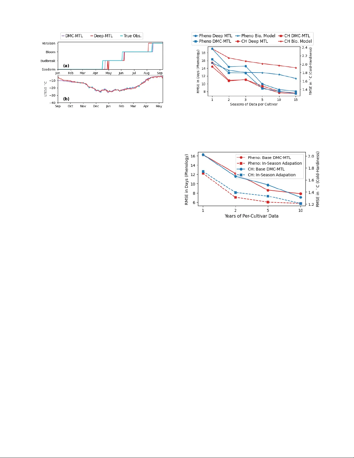
A Hybrid Modeling Framework f or Cr op Prediction T asks via Dynamic Parameter Calibration and Multi-T ask Lear ning William Solow 1 , Paola Pesantez-Cabr era 2 , Markus Keller 2 , La v Khot 2 , Sandhya Saisubramanian 1 , Alan Fer n 1 1 Oregon State Uni versity 2 W ashington State Uni versity { solo ww , sandhya.sai, afern } @ore gonstate.edu, { p.pesantezcabrera, mkeller , lav .khot } @wsu.edu Abstract Accurate prediction of crop states (e.g., phenol- ogy stages and cold hardiness) is essential for timely farm management decisions such as irriga- tion, fertilization, and canopy management to opti- mize crop yield and quality . While traditional bio- physical models can be used for season-long pre- dictions, they lack the precision required for site- specific management. Deep learning methods are a compelling alternativ e, but can produce biologi- cally unrealistic predictions and require large-scale data. W e propose a hybrid modeling approach that uses a neural network to parameterize a dif feren- tiable biophysical model and leverages multi-task learning for efficient data sharing across crop cul- tiv ars in data limited settings. By predicting the parameters of the biophysical model, our approach improv es the prediction accuracy while preserving biological realism. Empirical ev aluation using real- world and synthetic datasets demonstrates that our method improv es prediction accuracy by 60% for phenology and 40% for cold hardiness compared to deployed biophysical models. 1 Introduction Accurate forecasts of crop states are critical for growers to schedule time-sensitive farm operations such as cold stress mitigation, pruning, fertilization, irrigation, and harvesting for specialty crops [ Keller et al. , 2016; Milani and Cawley , 2024; Rogiers et al. , 2022 ] . Howe ver , accurate crop state prediction is challenging due to (1) limited av ailability of his- torical data for per-culti var calibration and sparse observa- tions during each growing season [ Zapata et al. , 2017 ] , and (2) the need to accurately model complex relationships be- tween daily weather features and crop states [ Guralnick et al. , 2024 ] . Existing approaches to this crop state prediction problem typically fall into two categories: mechanistic bio- physical models and data-dri ven deep learning approaches. Historically , biophysical models ha ve been used to model a v ariety of crop states, such as phenology (timing of each de- velopmental stage) and cold-hardiness (tolerance to lo w tem- peratures). Phenology is modeled by the Gro wing Degree Day (GDD) biophysical model based on daily accumulated heat units [ Parker et al. , 2013 ] . Cold hardiness models pre- dict the lethal bud temperature as a function of air tempera- ture and phenological stage [ Ferguson et al. , 2011 ] . Despite research supporting that crop states depend on exogenous weather features [ Greer et al. , 2006 ] , most specialty crop models only use air temperature as input, limiting their ex- pressiv eness [ Badeck et al. , 2004 ] . Further , current biophysi- cal models do not capture temporal nuances, such as how var - ied chilling hours in winter can change dormanc y release and phenological development [ Keller and T arara, 2010 ] ). These limitations affect their ability to produce accurate medium range (7-14 day) forecasts of the crop state [ Reynolds, 2022 ] . Deep learning offers a compelling alternative to biophys- ical modeling due to its ability to model complex, nonlin- ear , and temporal relationships between weather variables and crop physiological states. Howe ver , purely data-driv en models typically require large datasets and often produce bi- ologically unr ealistic predictions that violate kno wn physio- logical constraints on plant de velopment, such as predicting bud break after flo wering. This makes them unsuitable for actionable medium range forecasts [ Saxena et al. , 2023a ] . T o address the limitations of both deep learning and bio- physical modeling for crop state forecasting tasks, we present a hybrid approach that uses a recurrent network to dynam- ically refine the parameters of a differentiable biophysical crop model, based on daily weather (Figure 1). For example, giv en historical weather data and phenology observ ations, the network is trained to assign the base temperature for heat ac- cumulation in the GDD model such that the calibrated GDD model can accurately predict v arious phenological stages at deployment time. T o address limited per-culti var data, we use multi-task learning [ Caruana, 1997 ] to share information across cultiv ars and improv e prediction accuracy . While hybrid modeling techniques have been successfully applied to a v ariety of physical processes [ Jia et al. , 2021; Cai et al. , 2021 ] , they remain underexplored for crop state tasks. Prior h ybrid methods often approximate portions of the biophysical model [ V an Bree et al. , 2025 ] or predict residu- als [ V ijayshankar et al. , 2021 ] . In contrast, our approach pre- dicts parameters of the biophysical model, thereby producing biologically realistic and more accurate predictions. Scope, Contributions, and T rack Relevance This work is motiv ated by the operational needs of our primary Dormant BudBreak Bloom Ve ra i s o n Jan - Apr Apr - July July - Sept Pretrain ed RN N sel ect s dai ly p aramete rs of GDD model ( e.g . Te m p . S u m f o r B l o o m ) GDD Model Stage Predictions Wea th er Data Vineyard Man agement Operations Deploy frost mitigation Ta r g e t e d w a t e r stress Schedule labor for har ves t Apply fert il izer What vineyard operations to prepare for? Seasonal Phenologica l Stages Dynamic Model Calibr ation Pretrai ned RNN Dormant Bud Break Ve ra i s o n Bloom Day 1 … Day T -1 Day T Figure 1: Overview of our proposed method using phenology prediction as an example. In this case, seasonal phenological stages guide vineyard management operations. Our Dynamic Model Calibration via Multi-T ask Learning (DMC-MTL) approach uses a pretrained neural network and biophsyical model to produce high fidelity and biologically realistic phenology state forecasts. The pretrained RNN produces daily parameter predictions (Base T emperature, T emperature Sum for Bud Break, etc.) of the Growing Degree Day (GDD) phenology model which handles the daily stage prediction. stakeholders—specialty crop growers in the Pacific North- west (PNW) of the United States who face increasing risks from weather variability and climate stress [ Reynolds, 2022 ] . In this region, over $10 billion in annual specialty-crop pro- duction depends on timely and accurate crop state forecasts, including phenology and cold hardiness [ Knowling et al. , 2021 ] . Our team includes AI e xperts and agricultural domain experts who played key roles in data collection, selection of biophysical models, and system deployment. While our framework is broadly applicable to other crops, the paper focuses on wine grapes as a representati ve specialty crop and studies two critical crop states: phenology and cold har diness . W e train and validate our models using grape data collected in the PNW region between 1988-2025. Our primary contrib utions are: (1) presenting a novel hy- brid approach for accurate crop state forecasting by refin- ing parameters of the biophysical model conditioned on the weather features; (2) formulating the crop state prediction problem as a multi-task learning problem that lev erages data efficiently across grape cultiv ars; (3) presenting an in-season adaptation variant of our model; and (4) empirical ev aluations using real-w orld and synthetic datasets that demonstrate our approach’ s robustness and increased accuracy ov er state-of- the-art biophysical baselines, deep learning approaches, and hybrid models. Our model has recently been deployed on Ag- W eatherNet [ WSU, 2025 ] with ov er 26000 registered grow- ers. 2 Background and Related W ork Hybrid Modeling of Biophysical Processes Hybrid mod- eling combines deep learning and mechanistic modeling to obtain increasingly accurate and interpretable models of bio- physical processes [ W illard et al. , 2023 ] . Physics-Informed Neural Networks (PINNs) [ Raissi et al. , 2019 ] encode bio- logical constraints in the form of partial dif ferential equations into neural networks [ Karpatne et al. , 2017 ] enabling more accurate and biologically realistic predictions [ Karniadakis et al. , 2021 ] . In addition to PINNs, residual error hybrid mod- els use a deep learning model to predict the difference be- tween the true observ ation and the biophysical model predic- tion [ de Mattos Neto et al. , 2022 ] . Process replacement hy- brid models [ W ang et al. , 2023 ] replace a poorly understood aspects of the biophysical model with a neural network with wide applications to the natural sciences [ Feng et al. , 2022; Shen et al. , 2023 ] . T able 1 summarizes the characteristics of these models along different desiderate for crop state fore- casting tasks. Another related work is that of Unagar et al. (2021) that use reinforcement learning for parameter cal- ibration of a lithium battery . Howe ver , their problem setting assumes that the next true state of the system is known, which is untrue in our problem setting where medium range fore- casts are needed. W e adopt a supervised learning approach and train a network to dynamically modulate the parameters of the biophysical model in response to input features, en- abling medium horizon forecasts. Multi-T ask Learning When a set of tasks share similar structure, the multi-task learning [ Zhang and Y ang, 2018 ] framew ork can be used to efficiently aggregate data across tasks. Hard parameter sharing methods share a common set of hidden layers with unique prediction heads while soft pa- rameter sharing methods learn unique models but regularize weight updates to k eep models similar [ Ruder , 2017 ] . Shared embedding spaces [ Caruana, 1997 ] and task-specific embed- dings [ Changpinyo et al. , 2018 ] are viable methods for encod- ing task-specific information. W e empirically e valuate these approaches in data-limited setting across genetically di verse grape cultiv ars treated as separate tasks, assessing prediction accuracy for all culti vars. Machine Learning for Crop State For ecasts Saxena et al. (2023a) applied multi-task learning to grape bud break prediction using a classification model. Ho wever , this model made erroneous predictions (e.g., predicting the onset of dor - mancy after b ud break) that were inconsistent with biological processes. Saxena et al. (2023b) framed the grape cold hardi- Modeling Approach Biologically Realistic Exogenous Features T emporal Info. Biophysical Model ✓ ✗ ✗ Deep Learning ✗ ✓ ✓ PINN Sometimes ✓ ✓ Residual Sometimes ✓ ✓ Process Replacement ✓ ✗ ✗ DMC-MTL (Ours) ✓ ✓ ✓ T able 1: Modeling approaches for crop state forecasting tasks ev al- uated along different desiderata. PINN, Residual, Process Replace- ment, and DMC-MTL are all hybrid models. Biologically realistic means the model predictions reflect biological la ws. Exogenous fea- tur es means that the model output can be conditioned on additional weather features. T emporal info. indicates that the model can lev er- age historical input in addition to what the biophysical model uses. ness prediction problem as a multi-task learning problem and used a recurrent neural network (RNN) to improv e predic- tion accuracy over the deployed Ferguson biophysical model for cold hardiness [ Ferguson et al. , 2014 ] , demonstrating ef- ficacy of multi-task learning to lev erage data across culti vars. V an Bree et al. (2025) proposed a process replacement hy- brid model for bloom date in cherry trees by approximating the temperature response function in the GDD model with a neural network. Howe ver , their method did not consider the effect of exogenous weather features on phenology nor the temporal variation of heat accumulation. In contrast, our method leverages a RNN to both encode temporal and ex- ogenous weather information to av oid these limitations, and demonstrates state of the art performance in predicting grape phenology and matches grape cold hardiness while producing biologically realistic forecasts. 3 Dynamic Model Calibration Our problem setting and approach, D ynamic M odel C alibration with M ulti- T ask L earning (DMC-MTL), is in- spired by the following observations and hypotheses: (1) crop state prediction tasks are similar across cultiv ars, motiv ating our multi-task approach; (2) the parameters of crop state pre- diction models are hypothesized to vary over time based on historical weather in addition to the daily a verage tempera- ture; and (3) crop state forecasting requires biologically real- istic and accurate predictions. Problem Formulation W e formulate the problem of esti- mating dynamic parameters of a biophysical model as a time series supervised learning problem and adopt the multi-task setting. Let M ω denote the biophysical model with parame- ters ω . Let D i be the set of observ ed weather and daily crop states for each crop culti var i . Let S i,k be the k -th season in D i with S i,k = { W 0 , Y 0 , . . . , W T , Y T } where W t is the ob- served weather feature v ector and Y t is the observed crop state on day t . Given W ′ t ⊂ W t as input, M ω predicts a crop state Y ′ t . W e train a multi-task recurrent neural network model F θ that takes W t and culti var i.d. i as input, and outputs daily pa- rameters ω t of M . The resulting parameterized model M ω t , along with W ′ t , is used to generate crop state predictions Y ′ t . Giv en time series input S i,k , we use F θ and M to obtain a se- ℳ ! ! ℳ ! " ℱ " ℱ " 𝑊 # ’ 𝑌 $ ’ 𝑊 %&$ ’ 𝜔 # 𝜔 % 𝐻 # 𝐻 $ 𝐻 %&$ 𝐻 % (𝑖 , 𝑊 # ) 𝑌 % ’ … … (𝑖 , 𝑊 %&$ ) Figure 2: Network architecture of our approach DMC-MTL. The multi-task RNN ( F θ ) sequentially embeds cultiv ar i.d. i and con- catenates it with the daily weather features W t to predict a parame- terization ω t of the biophysical model M . Using the weather input to the biophysical model W ′ t and the daily parameterization ω t , crop state forecasts Y ′ t . . . Y ′ t + k can be generated. quence of parameter estimates ω 0 , . . . ω T and corresponding crop state predictions Y ′ 0 , . . . , Y ′ T (Figure 2). 3.1 Model Architecture The proposed model architecture for DMC-MTL is com- prised of three parts: the RNN-backbone, the multi-task model, and the parameterization of the biophysical model. The RNN-backbone ( f θ ) contains two linear layers, fol- lowed by a Gated Recurrent Unit (GR U) [ Chung et al. , 2014 ] , and another linear layer . T o support multi-task learning across cultiv ars, we define F θ which adds a linear embedding layer before f θ . This embedding layer con verts a one-hot en- coding of the cultiv ar into a dense v ector, which is concate- nated with the daily weather feature vector W t and passed to f θ , allowing the model to incorporate cultiv ar-specific infor- mation [ Saxena et al. , 2023b ] . ReLU acti vations are used, ex- cept for the final layer where a tanh activ ation is applied. The output of F θ , which is in the range [ − 1 , 1] , is then rescaled to match the parameter ranges of the biophysical model M (more details in Appendix A ). Figure 2 sho ws the daily parameterization ω t of the bio- physical model M , the core of our DMC-MTL approach. F θ makes causal parameter predictions by sequentially process- ing a weather data sequence W 0 , . . . , W T , generating corre- sponding parameters ω t at each time step. These parameters are used to parameterize M ω t and along with W ′ t , to produce phenology prediction Y ′ t +1 . Biophysical Model Implementation T o learn F θ , the bio- physical model M must be differentiable and implemented in a framework that supports gradient backpropagation. In practice, most specialty crop state models are relativ ely sim- ple and do not require advanced ordinary differential equa- tion solvers. W e additionally modify each biophysical model so that the parameters can be updated daily by F θ before each integration step. Parameters for the biophysical mod- els are known to lie in specified ranges. T o retain the abil- ity of the DMC-MTL approach to capture comple x depen- dencies among weather features, we choose large ranges for each parameter . See Appendix B for details of the biophysical models, con verting a biophysical model into a dif ferentiable framew ork, and the parameter ranges we consider . 4 Extending DMC-MTL: In-Season T uning Collecting suf ficient historical data for training accurate DMC-MTL models is challenging and often requires many years. In the case of insufficient data, it is beneficial to train the DMC-MTL model with av ailable data and then adjust the model parameters based on in-season observ ations made by growers in the field. T o enable in-season adaptation, er- r or signals are generated by comparing DMC-MTL model predictions with sparse in-season observations such as occa- sional measurements of bud stage or cold hardiness. These error signals are then used to adjust future predictions of bio- physical model parameters within the same growing season. This continual recalibration reduces bias accumulation seen in static prediction models and improv es prediction accurac y . When in-season observ ations are av ailable, the daily pa- rameter predictions made by the DMC-MTL approach are adjusted by using an additional neural network conditioned on error signals (Figure 3). While such Error Encoding Networks (EENs) hav e been used for video frame predic- tion [ Henaff et al. , 2017 ] , the y hav e not been explored for the sparse and low-dimensional error signals av ailable in crop state tasks. Furthermore, EENs hav e not previously been ap- plied to hybrid models, so we inv estigate their effecti veness in reducing in-season predictive error and recalibrating the hy- brid DMC-MTL model at small-to-medium horizon lengths. Model Architecture W e use an EEN with the same model architecture as DMC-MTL ( F θ ) giv en that observations are sparse and different cultiv ars may exhibit different error pat- terns. At each time step t the DMC-MTL model makes a prediction. If an in-season observation is av ailable, the dif- ference between the observation Y t and model prediction Y ′ t is passed to the EEN. If no observation is av ailable, the EEN input is zero. This is consistent with the observation that if the DMC-MTL model makes no error , then the EEN should not change the future model predictions of the biophysical model parameters. W e accomplish this by setting the bias terms within the EEN network layers to zero. EEN param- eter predictions are combined additively with the predicted parameters by the pretrained DMC-MTL and then passed to the biophysical model to predict the next crop state. T raining EENs Training the In-Season Adaptation model is a two step process. First, a DMC-MTL model is trained to predict parameters of the biophysical model that best predict the observ ed crop state. Then, the weights of the pretrained RNN F θ are frozen while the EEN is trained. The EEN is trained using the same training data as DMC-MTL, under the assumption that part of the observed crop state cannot be predicted solely by the weather and cultiv ar i.d. [ Henaff et al. , 2017 ] . W e use the historical crop state observations to mimic the availability of in-season observations in real time. W e randomly mask av ailable observ ations to ensure that the EEN does not learn rely on frequent observations for medium range forecasts, which may not be a vailable at deployment time (more details in Appendix A.2 ). 5 Experiment Setup The performance of our proposed DMC-MTL approach is ev aluated on two key criteria: (1) accurate and biologically Pretrai ned RNN s ele cts dai ly paramet ers of GDD mode l, modifi ed by EEN GDD Model Sparse Crop State Obser vation Pretrai ne d RNN EEN Wea t he r Data ( 𝑖, Error : [Obs . – Pre d .]) ⊕ Figure 3: In-Season Adaptation with DMC-MTL. Cultiv ar id i and error between observed and DMC-MTL predicted crop states are passed to the EEN. The parameters predicted by the EEN are com- bined additively to the prediction made by DMC-MTL ’ s pretrained RNN before parameterizing the biophyiscal model. realistic seasonal predictions and (2) efficient data use across cultiv ars. W e also considered (3) how in-season data can be used to reduce prediction error and (4) robustness to unex- pected subseasonal weather patterns, which can be demon- strated by e valuating a model on dif ferent weather distribu- tion. Based on these, we design our experiments to answer the following research questions: Q1 : (a) How does the average seasonal accuracy of DMC- MTL compare to deployed biophysical, deep learning and hybrid models? (b) Are predictions biologically re- alistic? Q2 : (a) Does DMC-MTL leverage data efficiently across cul- tiv ars? (b) Ho w much per-culti var data is required? Q3 : Do in-season crop state observations improv e DMC- MTL model predictions? Q4 : Does DMC-MTL exhibit robustness to dif ferent weather conditions compared to other baselines? Q5 : What percentage of cultiv ars are accurately predicted by each model type? 5.1 Datasets Real-W orld Datasets W e use the grape phenology and cold hardiness of 32 grape cultiv ars collected between 1988- 2025. Phenology (stages of bud break, bloom, and veraison) was observed daily during the non-dormant season, and cold hardiness was measured weekly , biweekly , or monthly during the dormancy season. There are between eight and 21 years of phenological data per culti var , and between four and 27 years of cold hardiness data per cultiv ar (43 to 797 samples). Pertinent historical open field weather data is sourced from AgW eatherNet [ WSU, 2025 ] . Appendix C includes a detailed description of the dataset and our data processing procedure. Processed real-world data will be made available upon paper acceptance; AgW eatherNet data is open-source. Synthetic Datasets T o explore the robustness of DMC- MTL to different weather conditions, we generated datasets with two biophysical crop models: (1) the GDD model with 31 cultiv ars [ Solow et al. , 2025 ] , and (2) the F erguson cold hardiness model with 20 culti vars [ Ferguson et al. , 2011 ] . W e Solution Approaches Grape Phenology Grape Cold Hardiness Q1a: DMC-MTL (Ours) 7.63 ± 3.56 1.21 ± 0.39 Bio. Model (Deployed) 18.58 ± 5.03 ∗ 2.03 ± 0.39 ∗ Bio. Model (Gradient Descent) 12.21 ± 5.13 ∗ 1.88 ± 0.42 ∗ Deep-MTL 8.16 ± 4.20 ∗ 1.30 ± 0.46 T empHybrid 9.84 ± 4.35 ∗ 3.45 ± 0.98 ∗ PINN 8.61 ± 4.32 ∗ 1.30 ± 0.43 Residual Hybrid 15.01 ± 6.00 ∗ 1.49 ± 0.52 ∗ Q2: DMC-STL 9.57 ± 3.79 ∗ 1.62 ± 0.34 ∗ DMC-Agg 9.81 ± 4.70 ∗ 1.51 ± 0.70 ∗ DMC-MTL-Mult 11.97 ± 4.43 ∗ 1.57 ± 0.53 ∗ DMC-MTL-Add 8.42 ± 3.56 ∗ 1.26 ± 0.41 DMC-MTL-MultiH 8.20 ± 4.15 ∗ 1.34 ± 0.48 ∗ T able 2: The average seasonal error (RMSE in days for phenology and ◦ C for cold hardiness) over all cultiv ars and five seeds in the testing set for grape phenology and cold hardiness. DMC-MTL is compared against two optimization procedures for the biophysical model, a deep learning approach, three hybrid models, and two DMC variants. Best-in-class results are reported in bold. A ∗ indicates that DMC-MTL yields a statistically significant impr ovement ( p < 0 . 05 ) using the paired t-test relativ e to the corresponding baseline. used historical weather data from the N ASAPower database for W ashington, USA [ N ASA, 2025 ] . W e also generated phe- nology and cold hardiness observations from V ermont, Cal- ifornia, and Oregon, USA. For each biophysical model, we generated ten years of data per culti var using the biophysi- cal models and historical NASA weather data. W e randomly masked 88% of the daily cold hardiness samples to resemble the real-world dataset. W e include code to generate this data. 5.2 Baselines, T raining and Evaluation Baselines W e consider 11 baselines for our experiments: (1) Deployed biophysical model —the GDD model for phe- nology and the F er guson model for cold hardiness that are used by our stakeholders; (2) Gr adient Descent on the bio- physical model parameters. T o the best of our kno wledge, this baseline has not been used before because the crop models hav e not been written in a dif ferentiable frame work; (3) T em- pHybrid —a hybrid model proposed by V an Bree et al. (2025) and adapted to the cold hardiness setting; (4) Deep-MTL — a multi-task model that either predicts probabilities for each phenological stage, or a continuous approximation of the cold hardiness. Instead of a tanh activ ation, there was a single out- put feature with no activ ation function. F or cold hardiness we used the re gression model proposed by Saxena et al. (2023b); (5) PINN —a Physics-informed neural network (PINN) with the same architecture and activ ation as the Deep-MTL model, trained with an additional loss term to weight biologically realistic predictions [ Aawar et al. , 2025 ] ; (6) Residual Hy- brid —a hybrid model that uses an RNN to predict the dif- ference between the biophysical model predictions and the observed crop state with the same network architecture as the Deep-MTL model [ V ijayshankar et al. , 2021 ] ; (7) DMC- STL —a DMC model without the embedding layer , trained on a per-culti var basis; (8) DMC-Ag g —a DMC model with- out the embedding layer and trained on all unlabeled cultiv ar data; (9) DMC-MTL-Mult —a DMC-MTL variant that uses a multiplicative embedding; (10) DMC-MTL-Add —a DMC- MTL v ariant that uses an additive embedding; (11) DMC- MTL-MultiH —a DMC-MTL v ariant that uses per-task pre- diction heads. See Appendix A for additional details. Baselines 1-6 to ev aluate the efficac y of our approach against the biophysical, hybrid and deep learning baselines. Baselines 7-11 ev aluate the efficac y of multi-task learning. Model T raining Protocol F or all experiments, we split the av ailable grape cultiv ar data into training and testing sets. T o build the test set, we withheld two seasons of data per cultiv ar from the training set. For the cultiv ars with the least amount of data, this resulted in two years of data in both the training and testing sets. Hyperparameters were selected using a v ali- dation set consisting of one season per cultiv ar . See Appendix D for more details on hyperparameter selection. Every model was trained for 400 epochs using a learning rate of 0.0002. W e decreased the learning rate by a factor of 0.9 after a 10 epoch plateau of the training loss. For the deep learning phenology model we used Cross Entropy loss and used PINN loss for the PINN hybrid model with p = 0 . 5 . F or all other models, we used the mean squared error loss function, masking days that did not hav e a ground truth observation. W e provide our code base here: https://tinyurl. com/IRAS- DMC- MTL. Evaluation Protocol W e trained each model five times with different data splits and reported the average root mean squared error (RMSE) across cultiv ars on the test sets. For phenology , the RMSE was the cumulativ e error in days over the predictions for bud break, bloom, and veraison. For cold hardiness we reported the RMSE in degrees Celsius ov er all unmasked samples during the testing year . 6 Results and Discussion Q1a: A verage Perf ormance of DMC-MTL T able 7 sho ws the average RMSE values for grape phenology and cold har- diness predictions using different approaches, across 32 cul- tiv ars. The results sho w that DMC-MTL dramatically out- performed the biophysical models that are currently used by growers in PNW re gion—the GDD model for phenology and Ferguson model for cold hardiness. DMC-MTL also im- prov ed o ver gradient descent optimization for both phenol- ogy and cold hardiness. These results indicate the importance of better optimization procedures for crop model calibration, Figure 4: DMC-MTL, Classification, and Regression model predic- tions for (a) grape phenology and (b) grape cold hardiness. DMC- MTL makes biologically realistic predictions while deep learning model predictions do not always respect biologicaly la ws. and how DMC-MTL can improv e upon standard practices. Further , DMC-MTL improved upon the Deep-MTL, T em- pHybrid, PINN, and Residual Hybrid models, demonstrating the importance of dynamic parameterization, inclusion of e x- ogenous weather features, and temporal information. W e per- formed the paired t-test aggregated over all culti vars to con- firm when our DMC-MTL performance improv ements were statistically significant ( p < 0 . 05) . Overall, our results indi- cate that our hybrid modeling approach is more accurate and reliable for predicting crop state tasks. Q1b: Biological Realism Biologically realistic predic- tions are critical for interpreting medium-range forecasts that growers rely on to plan their vineyard operations. Figure 4 shows that Deep-MTL model incorrectly predicts bloom, re- verts to bud break, then re-enters bloom three days later . Sim- ilarly , for cold hardiness, Deep-MTL overestimates the bio- logically plausible cold hardiness early in the growing season. In contrast, our DMC-MTL consistently makes biologically realistic crop state predictions. Q2a: Multi-T ask Data Sharing Results in T able 7 show that DMC-MTL outperforms DMC-STL and DMC-Agg, demonstrating that both single-task learning and nai ve aggre- gation are insuf ficient for these crop state prediction tasks. Other implementations of multi-task learning (DMC-MTL- Mult/Add/MultiH) exhibited lo wer prediction accuracy com- pared to DMC-MTL. These results demonstrate that our learned one-hot concatenation embedding approach best en- coded task-specific information, thereby efficiently leverag- ing data between cultiv ars. Additional results in Appendix E . Q2b: DMC-MTL Data Requirements T o ev aluate the per-culti var data requirements of DMC-MTL and compare its data efficienc y to other models, we v ary the number of seasons of av ailable per-culti var data from one to 15 during training. Our results in Figure 5 sho w that the a verage er- ror decreases across all model types, as more data becomes av ailable. While biophysical models seem to perform better in the lo w data regime, the deep models perform better with more data. In contrast, DMC-MTL outperforms both meth- ods across the entire range of data sizes. Figure 5: The performance of DMC-MTL models compared to deep learning and biophysical models under limited per-culti var training data for grape phenology (Pheno) and cold hardiness (CH). Results are av eraged o ver fiv e seeds using the same two-seasons-per -cultiv ar ev aluation sets. Figure 6: Performance of the base DMC-MTL with increasing per- cultiv ar data compared to the performance of the DMC-MTL with the additional in-season adaptation training for grape phenology (Pheno) and cold hardiness (CH). Results av eraged over fi ve seeds. Q3: In-Season Adaptation with In-Field Observations W e ev aluate the in-season adaptation with that of DMC-MTL, by incorporating real-time in-field data. Using the same train- ing data and protocol as the DMC-MTL models, we trained the in-season adaptation models with increasing amounts of per-culti var data. Figure 6 shows their performance on the same testing data. By using the in-season observations to re- fine parameters predicted by the DMC-MTL model, the EEN yields the most benefit where DMC-MTL prediction errors are highest (the most data-limited settings). W ith only one season of data per culti var , in-season adaptation reduces error by over 25%, enabling more actionable forecasts. As DMC- MTL accuracy improv es when additional data is av ailable during training, the benefit of the EEN diminishes, indicat- ing that in-season adaptation is most v aluable when historical per-culti var data is scarce. Q4: Robustness to Differing W eather Conditions Cur- rent crop models are calibrated on a site specific basis, lim- iting their applicability to regions with sufficient historical data. Further , they assume that weather conditions will re- main consistent and do not account for extreme weather ev ents which is critical for broader adoption. T o ev aluate our approach’ s robustness to varying weather conditions, we Phenology cold hardiness Approach W A (T rain Loc.) VT CA OR W A (T rain Loc.) VT CA OR DMC-MTL 5.9 ± 2.7 8.8 ± 5.6 30.4 ± 9.3 17.7 ± 0.5 0.42 ± 0.28 0.76 ± 0.31 1.37 ± 0.16 3.59 ± 0.24 Deep-MTL 6.1 ± 3.0 96.2 ± 10.8 120. ± 1.4 78.0 ± 1.9 0.34 ± 0.22 5.98 ± 1.57 6.01 ± 0.07 3.73 ± 0.46 PINN 5.3 ± 2.9 60.5 ± 14.2 59.8 ± 1.3 58.4 ± 3.9 0.39 ± 0.23 4.86 ± 1.41 8.38 ± 0.25 4.02 ± 0.40 T empHybrid 6.4 ± 5.2 97.3 ± 16.2 118. ± 20. 83.0 ± 18. 4.25 ± 0.98 5.60 ± 0.98 8.57 ± 1.14 6.43 ± 1.33 T able 3: RMSE (days and ◦ C ) for grape phenology and cold hardiness respectively , evaluated on unseen data sampled from the training location (W A) and from locations with a moderately similar weather (V ermont, California, and Oregon). Results averaged o ver fiv e seeds. Figure 7: Screenshot of the publicly accessible user interface on AgW eatherNet. The weather station-specific phenology forecasts during the 2025 season for the Cabernet Sauvignon cultiv ar of the Zapata (GDD-based biophysical model) are compared with the hy- brid (DMC-MTL) model. trained models on synthetic data from W ashington, USA, and ev aluated them on data from V ermont, Oregon, and Califor- nia, which hav e moderately similar weather patterns. Exper- iments were performed using synthetic phenology and cold hardiness datasets. T able 3 shows the cumulative RMSE in days on the W ashington test set and V ermont, Oregon, and California test sets. While all models performed similar on the W ashington test set, deep learning and other hybrid mod- els produced large errors on the V ermont, Oregon, and Cal- ifornia test sets. In contrast, DMC-MTL had a marginal in- crease in error on the test set, demonstrating rob ustness to varying weather conditions and its ability to produce usable predictions in unseen weather conditions. Q5: Accuracy of Per -Cultiv ar Predictions While DMC- MTL substantially reduces prediction error compared to bio- physical models, its practical adoption depends on growers’ error tolerance. T o assess the potential model use, we ev alu- ate the proportion of cultiv ars with RMSE belo w predefined thresholds, reflecting varying tolerance le vels. W e vary the RMSE tolerance threshold in the range [0 , 2 . 5] for cold har - diness and [0 , 30] for phenology . Our results in Figure 8 show that DMC-MTL consistenly performs better than the baselines for both phenology and cold hardiness. In addi- tion, DMC-MTL ’ s biologically realistic predictions position its medium range forecasts to be predicted unambiguously , positioning it to be widely used in the field. Figure 8: Percentage of all cultiv ars with cumulative error below a giv en RMSE threshold modeling a grape gro wer’ s tolerance for model prediction error. Results are reported over fiv e seeds for (a) phenology and (b) cold hardiness. 7 Deployment of DMC-MTL Models DMC-MTL models for grape phenology were recently de- ployed on AgW eatherNet [ WSU, 2025 ] for the 2026 grow- ing season. Figure 7 is a screenshot of the user interface visible to growers, showing our model predictions for a spe- cific weather station and grape cultiv ar (Cabernet Sauvignon) and that of the Zapata model (a GDD-based model that we compared against in T able 7) [ Zapata et al. , 2017 ] . Stake- holders in the PNW widely use AgW eatherNet and will have access to both DMC-MTL and biophysical model forecasts to inform their vine yard operations which we will monitor for long-term impact. Continued analysis of deployed DMC- MTL models will provide insights to viticulturists on our in- terdisciplinary team to better understand the shortcomings of deployed biophysical models and improv e understanding of grape phenological dev elopment. 8 Conclusion and Future W ork W e present a no vel deep learning method that predicts the pa- rameters of biophysical models. Our results show that lev er- aging the benefits of both deep network architecture and bio- physical models can outperform both methods individually . In very data-limited settings, our in-season adaptation method provides gro wers with a more accurate prediction tool that is especially beneficial when waiting for more data is not feasi- ble. Future work will aim to develop uncertainty quantifica- tion methods for crop state tasks through our hybrid modeling framew ork. Acknowledgments The authors thank L ynn Mills and Zilia Khaliullina at the Irri- gated Agriculture Research and Extension Center (IAREC), W ashington State Univ ersity , for their in valuable support in collecting and sharing grape phenology data. The authors would also like to thank Sanjita Bhavirisetty , Jaitun Patel, and Dheeraj V urukuti for their assistance in the deployment of DMC-MTL phenology models on AgW eatherNet. This research was supported by USD A NIF A aw ard No. 2021- 67021-35344 (AgAID AI Institute). References [ Aawar et al. , 2025 ] Majd Al Aaw ar, Srikar Mutnuri, Man- sooreh Montazerin, and Ajitesh Sriv astav a. Dynamics- Based Feature Augmentation of Graph Neural Networks for V ariant Emergence Prediction. In Proceedings of the AAAI Conference on Artificial Intelligence , volume 39, pages 27793–27801, April 2025. [ Allen, 1994 ] P . Geoffrey Allen. Economic forecasting in agriculture. International J ournal of F orecasting , 10(1):81–135, June 1994. [ Badeck et al. , 2004 ] Franz-W . Badeck, Alberte Bondeau, Kristin B ¨ ottcher , Daniel Doktor , W olfgang Lucht, J ¨ org Schaber , and Stephen Sitch. Responses of spring phenol- ogy to climate change. New Phytologist , 162(2):295–309, 2004. [ Cai et al. , 2021 ] Shengze Cai, Zhicheng W ang, Sifan W ang, Paris Perdikaris, and Geor ge Em Karniadakis. Physics- Informed Neural Networks for Heat Transfer Problems. Journal of Heat T ransfer , 143(060801), April 2021. [ Caruana, 1997 ] Rich Caruana. Multitask Learning. Ma- chine Learning , 28(1):41–75, July 1997. [ Changpinyo et al. , 2018 ] Soravit Changpin yo, Hexiang Hu, and Fei Sha. Multi-T ask Learning for Sequence T agging: An Empirical Study. In International Confer ence on Com- putational Linguistics , August 2018. [ Chung et al. , 2014 ] Junyoung Chung, Caglar Gulcehre, KyungHyun Cho, and Y oshua Bengio. Empirical Evalu- ation of Gated Recurrent Neural Networks on Sequence Modeling. In NIPS 2014 W orkshop on Deep Learning and Repr esentation Learning , December 2014. [ de Mattos Neto et al. , 2022 ] Paulo S. G. de Mattos Neto, George D. C. Cav alcanti, Domingos S. de O. Santos J ´ unior, and Eraylson G. Silv a. Hybrid systems using resid- ual modeling for sea surface temperature forecasting. Sci- entific Reports , 12(1):487, January 2022. [ Feng et al. , 2022 ] Dapeng Feng, Jiangtao Liu, Kathryn Lawson, and Chaopeng Shen. Different iable, Learn- able, Regionalized Process-Based Models W ith Multi- physical Outputs can Approach State-Of-The-Art Hydro- logic Prediction Accuracy . W ater Resources Resear ch , 58(10):e2022WR032404, 2022. [ Ferguson et al. , 2011 ] John C. Ferguson, Julie M. T arara, L ynn J. Mills, Gary G. Gro ve, and Markus Keller . Dy- namic thermal time model of cold hardiness for dormant grapevine buds. Annals of Botany , 107(3):389, January 2011. [ Ferguson et al. , 2014 ] John C. Ferguson, Michelle M. Moyer , L ynn J. Mills, Gerrit Hoogenboom, and Markus Keller . Modeling Dormant Bud Cold Hardiness and Bud- break in T wenty-Three V itis Genotypes Rev eals V ariation by Region of Origin. American J ournal of Enology and V iticulture , 65(1):59–71, March 2014. [ Greer et al. , 2006 ] Dennis H. Greer , Jens N. W ¨ unsche, Cara L. Norling, and Harry N. W iggins. Root-zone tem- peratures af fect phenology of bud break, flower cluster de- velopment, shoot e xtension gro wth and gas e xchange of ’Braeburn’ (Malus domestica) apple trees. T r ee Physiol- ogy , 26(1):105–111, January 2006. [ Guralnick et al. , 2024 ] Robert Guralnick, Theresa Crim- mins, Erin Grady , and Lindsay Campbell. Phenological re- sponse to climatic change depends on spring warming ve- locity . Communications Earth & En vir onment , 5(1):634, October 2024. [ Henaff et al. , 2017 ] Mikael Henaff, Junbo Zhao, and Y ann LeCun. Prediction Under Uncertainty with Error- Encoding Networks. , Nov ember 2017. [ Jia et al. , 2021 ] Xiaowei Jia, Jared W illard, Anuj Karpatne, Jordan S. Read, Jacob A. Zwart, Michael Steinbach, and V ipin Kumar . Physics-Guided Machine Learning for Scientific Discovery: An Application in Simulating Lake T emperature Profiles. A CM/IMS T rans. Data Sci. , 2(3):20:1–20:26, May 2021. [ Karniadakis et al. , 2021 ] George Em Karniadakis, Ioan- nis G. K evrekidis, Lu Lu, Paris Perdikaris, Sifan W ang, and Liu Y ang. Physics-informed machine learning. Na- tur e Reviews Physics , 3(6):422–440, June 2021. [ Karpatne et al. , 2017 ] Anuj Karpatne, Gowtham Atluri, James Faghmous, Michael Steinbach, Arindam Baner- jee, Auroop Ganguly , Shashi Shekhar , Nagiza Sama- tov a, and V ipin Kumar . Theory-guided Data Science: A New Paradigm for Scientific Discovery from Data. IEEE T ransactions on Knowledge and Data Engineering , 29(10):2318–2331, October 2017. [ Keller and T arara, 2010 ] Markus Keller and Julie M. T arara. W arm spring temperatures induce persistent season-long changes in shoot dev elopment in grapevines. Annals of Botany , 106(1):131–141, July 2010. [ Keller et al. , 2016 ] Markus Keller , Pascual Romero, He- mant Gohil, Russell P . Smithyman, W illiam R. Riley , L. Federico Casassa, and James F . Harbertson. Deficit Ir- rigation Alters Grape vine Growth, Physiology , and Fruit Microclimate. American Journal of Enology and V iticul- tur e , 67(4):426–435, October 2016. [ Knowling et al. , 2021 ] Matthew J. Knowling, Bree Bennett, Bertram Ostendorf, Seth W estra, Rob R. W alker , Anne Pellegrino, Everard J. Edwards, Cassandra Collins, V inay Pagay , and Dylan Grigg. Bridging the gap between data and decisions: A revie w of process-based models for viti- culture. Agricultural Systems , 193:103209, October 2021. [ Lorenz et al. , 1995 ] D.h. Lorenz, K.w . Eichhorn, H. Blei- holder , R. Klose, U. Meier , and E. W eber . Growth Stages of the Grapevine: Phenological growth stages of the grapevine (V itis vinifera L. ssp. vinifera)—Codes and descriptions according to the extended BBCH scale. Aus- tralian Journal of Grape and W ine Researc h , 1(2):100– 103, 1995. [ Milani and Cawle y , 2024 ] Alejandro Milani and Alejan- dro Mac Cawley . Analyzing the impact of forecast errors in the planning of wine grape harvesting operations using a multi-stage stochastic model approach. , May 2024. [ N ASA, 2025 ] N ASA. Nasapo wer database. https://power . larc.nasa.gov/, 2025. [ Parker et al. , 2013 ] Amber Parker , Inaki Garcia De Cort ´ azar-Atauri, Isabelle Chuine, G ´ erard Barbeau, Ben- jamin Bois, Jean-Michel Boursiquot, Jean-Yves Cahurel, Marion Claverie, Thierry Dufourcq, Laurence G ´ eny , Guy Guimberteau, Rainer W . Hofmann, Oli vier Jacquet, Thierry Lacombe, Christine Monamy , Hernan Ojeda, Lau- rent Panig ai, Jean-Christophe Payan, Bego ˜ na Rodriquez Lov elle, Emmanuel Rouchaud, Christophe Schneider , Jean-Laurent Spring, Paolo Storchi, Diego T omasi, W illiam Trambouze, Michael T rought, and Cornelis V an Leeuwen. Classification of varieties for their timing of flowering and veraison using a modelling approach: A case study for the grape vine species V itis vinifera L. Agricultural and F or est Meteor ology , 180:249–264, October 2013. [ Paszke et al. , 2017 ] Adam P aszke, Sam Gross, Soumith Chintala, Gregory Chanan, Edward Y ang, Zachary De- V ito, Zeming Lin, Alban Desmaison, Luca Antiga, and Adam Lerer . Automatic dif ferentiation in pytorch. In NIPS-W orkshop , 2017. [ Raissi et al. , 2019 ] M. Raissi, P . Perdikaris, and G. E. Kar- niadakis. Physics-informed neural networks: A deep learning framework for solving forward and inv erse prob- lems in volving nonlinear partial dif ferential equations. Journal of Computational Physics , 378:686–707, Febru- ary 2019. [ Reynolds, 2022 ] Andrew G. Reynolds. 11 - V iticultural and vineyard management practices and their effects on grape and wine quality . In Managing W ine Quality (Second Edition) , pages 443–539. W oodhead Publishing Series in Food Science, T echnology and Nutrition, January 2022. [ Rogiers et al. , 2022 ] Suzy Y . Rogiers, Dennis H. Greer , Y in Liu, T intu Baby , and Zeyu Xiao. Impact of climate change on grape berry ripening: An assessment of adaptation strategies for the Australian vineyard. F r ontiers in Plant Science , 13:1094633, December 2022. [ Ruder , 2017 ] Sebastian Ruder . An Overvie w of Multi-T ask Learning in Deep Neural Networks. , June 2017. [ Rudin, 2019 ] Cynthia Rudin. Stop explaining black box machine learning models for high stakes decisions and use interpretable models instead. Natur e Machine Intelligence , 1(5):206–215, May 2019. [ Salazar-Guti ´ errez and Chav es-Cordoba, 2020 ] M.R. Salazar-Guti ´ errez and B. Chaves-Cordoba. Model- ing approach for cold hardiness estimation on cherries. Agricultural and F or est Meteorolo gy , 287:107946, June 2020. [ Saxena et al. , 2023a ] Aseem Saxena, Paola Pesantez- Cabrera, Rohan Ballapragada, Markus Keller , and Alan Fern. Multi-T ask Learning for Budbreak Prediction. arXiv:2301.01815 , January 2023. [ Saxena et al. , 2023b ] Aseem Saxena, Paola Pesantez- Cabrera, Rohan Ballapragada, Kin-Ho Lam, Markus Keller , and Alan Fern. Grape Cold Hardiness Prediction via Multi-T ask Learning. In Pr oceedings of the AAAI Confer ence on Artificial Intelligence , volume 37, pages 15717–15723, 2023. [ Seidel et al. , 2018 ] S. J. Seidel, T . Palosuo, P . Thorburn, and D. W allach. T ow ards improved calibration of crop models – Where are we now and where should we go? Eur opean Journal of Agr onomy , 94:25–35, March 2018. [ Shen et al. , 2023 ] Chaopeng Shen, Alison Appling, Pierre Gentine, T oshiyuki Bandai, Hoshin Gupta, Alexandre T artakovsky , Marco Baity-Jesi, Fabrizio Fenicia, Daniel Kifer , Xiaofeng Liu, Li Li, Dapeng Feng, W ei Ren, Y i Zheng, Ciaran Harman, Martyn Clark, Matthe w Far - thing, and Prav een Kumar . Dif ferentiable modeling to unify machine learning and physical models and advance Geosciences. , May 2023. [ Solow et al. , 2025 ] W illiam Solow , Sandhya Saisubrama- nian, and Alan Fern. W ofostgym: A crop simulator for learning annual and perennial crop management strategies. In Reinfor cement Learning Confer ence (RLC) 2025 , 2025. [ Sundararajan et al. , 2017 ] Mukund Sundararajan, Ankur T aly , and Qiqi Y an. Axiomatic attribution for deep net- works. In Proceedings of the 34th International Confer - ence on Machine Learning (ICML 2017) , pages 3319– 3328. PMLR, 2017. [ Unagar et al. , 2021 ] Ajaykumar Unagar , Y uan Tian, Manuel Arias Chao, and Olga Fink. Learning to Calibrate Battery Models in Real-T ime with Deep Reinforcement Learning. Ener gies , 14(5):1361, January 2021. [ V an Bree et al. , 2025 ] Ron V an Bree, Diego Marcos, and Ioannis N. Athanasiadis. Hybrid Phenology Modeling for Predicting T emperature Effects on T ree Dormancy . In Pr o- ceedings of the AAAI Conference on Artificial Intelligence , volume 39, pages 28458–28466, April 2025. [ van Diepen et al. , 1989 ] C.a. v an Diepen, J. W olf, H. v an Keulen, and C. Rappoldt. WOFOST: A simulation model of crop production. Soil Use and Manag ement , 5(1):16– 24, 1989. [ V ijayshankar et al. , 2021 ] Sanjana V ijayshankar , Jennifer King, and Peter Seiler . W ind Power F orecasting using LSTMs. In 2021 60th IEEE Confer ence on Decision and Contr ol (CDC) , pages 3658–3663, December 2021. [ W ang et al. , 2023 ] Pengfei W ang, Ze Zhu, W enlong Liang, Longtao Liao, and Jiashuang W an. Hybrid mechanistic and neural network modeling of nuclear reactors. Ener gy , 282:128931, Nov ember 2023. [ W illard et al. , 2023 ] Jared W illard, Xiaowei Jia, Shaoming Xu, Michael Steinbach, and V ipin K umar . Integrating Sci- entific Knowledge with Machine Learning for Engineering and En vironmental Systems. A CM Computing Surveys , 55(4):1–37, April 2023. [ WSU, 2025 ] WSU. Agweathernet. https://weather .wsu.edu, 2025. [ Zapata et al. , 2017 ] Diana Zapata, Melba Salazar- Gutierrez, Bernardo Chaves, Markus Keller , and Gerrit Hoogenboom. Predicting Key Phenological Stages for 17 Grapevine Culti vars (V itis vinifera L.). American Journal of Enology and V iticulture , 68(1):60–72, January 2017. [ Zhang and Y ang, 2018 ] Y u Zhang and Qiang Y ang. An ov erview of multi-task learning. National Science Revie w , 5(1):30–43, January 2018. A ppendix A: Model Architectur es In this section we provide additional information on the DMC-MTL model and the v ariants that we used as experi- ment baselines. Appendix A.1: DMC Models The DMC-MTL model is composed of three parts, the RNN- Backbone (Figure 2a), the multi-task embedding (Figure 2b) and the interaction between the deep learning model and the biophysical model (Figure 2c), encapsulating our pro- posed DMC-MTL approach. For all DMC architectures (DMC-MTL, DMC-STL, DMC-Agg, and multi-task vari- ants), we used a Gated Recurrent Unit (GR U) with 1024 hid- den units [ Chung et al. , 2014 ] . The linear layers were reduced by factors of tw o: the first linear layer before the GR U was 256 hidden units, the second was 512 hidden units. After the GR U, the first linear layer was 512 hidden units and the sec- ond was 256 hidden units before making a prediction of the biophysical model parameters. Across all e xperiments, the embedding layer in F θ was the same size as the number of input features (16 for the real-world datasets and 11 for the synthetic datasets). In contrast to DMC-MTL, DMC-STL and DMC-Agg did not ha ve a multi-task embedding, and only utilized the RNN- backbone f θ and the additional linear layer following f θ . DMC-STL models were trained using data from only a sin- gle cultiv ar . Meanwhile, DMC-Agg models were trained on unlabeled data aggregated across all cultiv ars. For our exper - iments, this meant that we trained fi ve DMC-STL models per cultiv ar , whereas we only trained fiv e DMC-Agg models per domain (i.e., phenology , cold-hardiness, wheat yield). Appendix A.2 Error Encoding Network Architectur e The Error Encoding Networks (EENs) used in the in-season adaptation experiments use similar model architecture as DMC-MTL models. The input to the ENNs are the error sig- nal (a scalar) and the cultiv ar i.d. i . In the same fasion as the DMC-MTL models, the one-hot embedding of the culti- var serves to distinguish between different error patterns that may vary between cultiv ars. Howe ver , giv en that the error signal is a scalar , the one-hot embedding is also a real-v alued scalar , to avoid the cultiv ar embedding information dominat- ing the error signal passed to f θ . The size of the first linear layer is adjusted to account for this change in input size, oth- erwise the layer sizes remain the same as DMC-MTL. If, during a gro wing season, the EEN observ es no error between the observ ation and prediction made by the DMC- MTL model, then it should not modify the future parameters predicted by the DMC-MTL network. In this case, we can assume that the DMC-MTL model is predicting the observed data optimally , and no recalibration is needed. T o accomplish this, the network layers of the EEN do not contain any bias terms, and when the observed error is zero, we zero out the one-hot culti var embedding as well. As a result, the EEN learns to quickly recalibrate the parameters predicted by the DMC-MTL model (and thus adjust the internal state of the biophysical model) for future in-season predictions. Henaff et al. (2017) observed that in many cases, the de- sired prediction (in their case ne xt video frame prediction) can be decomposed into a deterministic and stochastic por- tion, motiv ating the study of EENs to handle the stochastic prediction portion conditioned on pre viously observed error . In the crop state prediction task, the deterministic portion is explained by the weather and cultiv ar i.d. while we hy- pothesize that the stochastic portion can be explained by the sparsely observed error . Instead of learning an additi ve la- tent state, we instead learn parameters which are added to the predicted parameters of the pretrained DMC-MTL model that are then passed to the biophysical model to make the next crop state prediction. Giv en that the EEN and DMC-MTL model have different inputs, it is appropriate to train the EEN model on the same training data as the DMC-MTL model, while freezing the weights of the DMC-MTL model during EEN training. As a result, the EEN learns to correct the error made by a specific DMC-MTL model. As shown in our results, this framing ef- fectiv ely reduces av erage prediction error in low data settings. T o av oid relying on future in-season observations, during we randomly select a day t for each season in the batch after which the EEN receiv es no further observations. Appendix A.3 Multi-T ask Learning V ariants In our experiments, we tested four approaches to embedding embedding task-specific culti var information into our multi- task models. W e expand on these methods belo w: 1. DMC-MTL is our best performing model across all datasets and uses a concatenation embedding based on a one-hot embedding of the cultiv ar . This embedding is the dimensionality of the weather features (16 for real- world data and 11 for synthetic data) and is concatenated on to the weather data as shown in Figure 2b before be- ing fed into the first fully connected layer and subse- quently the GR U. 2. DMC-MTL-Add uses the same learnable one-hot embed- ding as DMC-MTL. Howe ver , this embedding vector is added to the weather vector instead of concatenated be- fore being fed into the first fully connected layer . Thus, between DMC-MTL-Add and DMC-MTL, the first fully connected layer has a differing input size. 3. DMC-MTL-Mult uses the same approach as DMC- MTL-Add, b ut instead multiplies the weather informa- tion by the learnable embedding vector . 4. DMC-MTL-MultiH uses different fully connected lay- ers for each cultiv ar as prediction heads. This architec- ture shares the same structure as DMC-MTL (Figure 2b) with the exception that there are 31 fully connected lay- ers for phenology and 20 for cold-hardiness instead of a single output layer . Each final fully connected layer is trained only on the per -cultiv ar information, while the rest of the layers are trained in unison on all data. These four approaches encompass hard parameter shar- ing and embedding methods fundamental to multi-task learn- ing [ Zhang and Y ang, 2018 ] . Thus, along with DMC-STL and DMC-Agg variants described in the main text, they rep- resent a comprehensi ve study on the utilty of multi-task learn- ing in our proposed hybrid modeling frame work. Appendix A.4 Deep Learning Models The deep learning models (RNN with classification and re- gression targets) used the same network architecture as DMC- MTL ( F θ ) as suggested by Sax ena et al. (2023b). Howe ver , instead of using 1024 hidden units for the GR U, we used 2048 hidden units and scaled the linear layers accordingly (see Figure 2b). The prediction tar get for the cold-hardiness and WOFOST wheat yield experiments (see Appendix B.4 ) was a regression approximation of the crop state. For grape cold-hardiness prediction target was not just the L TE50, but also the L TE10 and L TE90 as well (the lethal temperatures at which 10% and 90% of dormant grape bud die, respectively) with the training loss as the sum of the MSE v alues across the L TE50, L TE10, and L TE90 observations. In practice, we found that this extra L TE10 and L TE90 data was unneeded to make accurate predictions of L TE50. For grape phenology we used a classification target of four classes corresponding to dormancy , bud break, bloom, and veraison. For the re gres- sion tasks we used mean squared error (MSE) loss and for the classification task we used Cross Entropy Loss with soft- max activ ation to obtain the highest probability of a specific phenological stage. Appendix A.5 Hybrid Models Physics Inf ormed Neural Network The PINN models used a network architecture identical to the deep learning models (Figure 2b) using a stage-based classification tar get for grape phenology and regression target for cold-hardiness and wheat yield. Unlike the deep learning models, the PINN models were trained using a physics-informed loss based on the biophysical model outputs to penalize biologically unre- alistic predictions [ Aawar et al. , 2025 ] : L P I N N = 1 − p N N X i =1 ( ˆ y i − y i ) 2 + p N N X i =1 ( ˆ y i − ˙ y i ) 2 where y i was the observed crop state, ˆ y i was the crop state prediction of the PINN, and ˙ y i was the crop state prediction of the biophysical model based on the best stationary model parameters. W e found empirically that p = 0 . 5 produced the best phenology predictions, and used that value in our cold- hardiness and wheat yield results. Residual Error Hybrid Model Residual error hybrid mod- els combine a primary biophysical model with an auxiliary deep learning model to learn the structure of the remaining forecast error . Instead of assuming that the base biophys- ical model captures all predictiv e information, this hybrid approach explicitly learns the structure of the residual error with a deep learning approach. By reducing the scope that the data-dri ven model needs to learn, predictiv e accuracy and generalization is impro ved as the biophysical model provides the majority of the prediction structure. W e use the model architecture described in Figure 2b. The biophysical model has per-cultiv ar parameters calibrated with Bayesian Optimization or brute force [ Solow et al. , 2025; Ferguson et al. , 2014 ] . The output of the biophysical model is added to the output of the deep learning model and the sum of both terms is used in the loss function for training F θ . T empResponse Hybrid Model The temperature response hybrid model for phenology [ V an Bree et al. , 2025 ] replaces the temperature response function in the GDD phenology model with a small feedforward neural network. This design choice is based on the observation that man y GDD model variants change the temperature response function which adds bias to the model. Instead V an Bree et al. (2025) suggest to make this temperature response function learnable, reduc- ing the bias in model choice selection. See Appendix C.1 for a description of the temperature response function. In the T empResponse hybrid model, the GDD model is im- plemented in a dif ferentiable frame work [ Paszke et al. , 2017 ] and gradient descent is performed both on the neural network parameters and GDD model parameters to learn the best fit model parameters and temperature response function. While the T empResponse hybrid model was originally de- fined for tree phenology , we modified it to function with the Ferguson cold-hardiness model as well [ Ferguson et al. , 2014 ] . The biophysical Fer guson cold-hardiness model mod- els two stages of dormancy with a transition occurring when sufficient chilling units are reached [ Ferguson et al. , 2011 ] . The chilling accumulation function is approximated by a small feedforward neural network in the same way that the temperature response function in the GDD model is learned. Thus, in the T empResponse hybrid model for cold-hardiness, we perform gradient descent on both the neural network pa- rameters and Ferguson cold-hardiness model parameters to learn the best fit model. A ppendix B: Biophysical Model Descriptions Before a biophysical model is used for agricultural crop state prediction, it must be calibrated with historical data. Com- mon approaches used in the agricultural community for pa- rameter calibration include brute force search [ Ferguson et al. , 2014 ] , regression techniques [ Zapata et al. , 2017 ] , and Bayesian optimization [ Seidel et al. , 2018 ] . Howe ver , these approaches assume that a stationary par ameter set best ex- plains the observed time series data during the growing sea- son. Recent work has sho wn that early spring warming im- pacts phenology [ Guralnick et al. , 2024 ] , indicating that a stationary heat accumulation model is insuf ficient and it is well understood that other weather features impact phenol- ogy [ Greer et al. , 2006; Badeck et al. , 2004 ] . Our approach addresses both of these concerns by conditioning phenology on exogenous weather features via daily parameter calibra- tion. Belo w we describe the PyT orch implementation to con- vert biophysical models into a differentiable framew ork, the biophysical models, and the parameters of the models that are calibrated using our DMC-MTL approach. A ppendix B.1: PyT or ch Implementation T o create differentiable implementations, we replace all mathematical operation in each biophysical model with the corresponding PyT orch operation so that gradients are tracked. Parameters, states, and rates are instantiated as ten- sors instead of floats. T o enable batch learning, all conditional statements are replaced by ‘where’ statements. A ppendix B.2: Gro wing Degree Day Phenology Model Grape phenology is described by the Eichhorn-Lorenz phe- nological stages [ Lorenz et al. , 1995 ] and includes three key phenological states: bud break, bloom, and veraison. Accu- rate prediction of these three states enable gro wers to follow crop management policies more precisely in order to increase yield and quality , and to increase vineyard efficienc y by en- suring farm labor is a vailable during the gro wing season. The Gro wing Degree Day (GDD) model is a mechanistic phenology model that makes predictions from January 1st un- til September 7th, for the three key phenological stages [ Zap- ata et al. , 2017 ] . The GDD model accumulates the amount of Degree Days (DD) needed to transition between phenological stages. Giv en a base temperature value T b , and a maximum effecti ve temperature T m , the degree days can be computed: D D = H X i =1 min  T m , ( T i − T b )  where H is the length of the season and the term inside the summand is the temperature response function. A stage transition occurs when DD is greater than a specific threshold. Each stage, b ud break, bloom, and veraison, has an associated threshold v alue. In T able 4 we list the sev en parameters of the GDD model and the associated ranges that we chose to use in the DMC method for normalizing parameters after the tanh activ ation. A ppendix B.3: F erguson Cold-Hardiness Model Description Grape cold-hardiness characterizes the grape vine’ s resistance to lethal cold temperatures from September 7th to May 15th [ Ferguson et al. , 2011 ] . When cold-hardiness is lo w in the spring and fall, sudden frost e vents can cause significant damage to to dormant b uds resulting in a decrease in yield quantity . Cold-hardiness is difficult to measure in the field; consequently , grape gro wers rely on the Fer guson model for daily predictions of L TE50, the temperature when 50% of dormant buds freeze [ Ferguson et al. , 2014 ] . By contrasting the L TE50 predictions with the weather forecast, grape grow- ers decide whether prev entative measures (e.g., wind ma- chines and heaters) are needed to protect the dormant buds. The Ferguson model computes the change in L TE50, ∆ H c , as a function of daily acclimation and deacclimation based on dormancy stage and ambient temperature. See Ferguson et al. (2011) for a complete description. The Ferguson model parameters that we calibrate in our approach and the corre- sponding ranges are listed in T able 4. A ppendix B.4: WOFOST Wheat Model Description As an additional testing domain to complement phenology and cold-hardiness, we consider the wheat yield domain. Ac- curate forecast of staple crop yields are critical to financial planning. The WOFOST crop gro wth model [ van Diepen et al. , 1989 ] is widely used to predict field level yield for many crops, including winter wheat, by predicting the daily yield (as the daily weight of the storage organs) from January 1st to September 1st each year . Predicting hectare-lev el wheat yield is critical for economi- cal planning [ Allen, 1994 ] . Using historical weather data, the WOFOST model can generate synthetic wheat yield observ a- tions. The WOFOST model is a significantly more compli- cated model compared to the phenology and cold-hardiness models. While creating a PyT orch implementation required upfront work, our results demonstrate that our hybrid ap- proach significantly outperforms other modeling approaches for the prediction of winter wheat yield during the gro wing season. A ppendix C: Datasets Details In this section we discuss the real-world data used in our ex- periments. A ppendix C.1: Real W orld Data As mentioned in the main text, our experiments are conducted in a data-limited setting. The cold-hardiness and phenology from up to 32 genetically di verse cultiv ars/genotypes of field- grown grape vines has been measured since 1988 in the labo- ratory of the WSU Irrigated Agriculture Research and Exten- sion Center in Prosser , W A (46.29°N latitute; -119.74°W lon- gitude). In the vineyards of the IAREC, the WSU-Roza Re- search Farm, Prosser , W A (46.25°N latitude; -119.73°W lon- gitude), and in the cultiv ar collection of Ste. Michelle W ine Estates, Paterson, W A (45.96°N latitute; -119.61°W longi- tude), cane samples containing dormant buds were collected daily , weekly , or at 2-week intervals from leaf fall in autumn to bud swell in spring while phenological stage observations (onset of b ud break, bloom, and v eraison) were observed dur - ing from bud swell to leaf f all. Phenology was observed daily . T able 5 sho ws a summary of the number of years of phe- nology data and the number of cold-hardiness samples col- lected per cultiv ar after data processing. In addition to the cold-hardiness and phenology measurements, the real-world weather data from nearby open-field weather station was used and contains 14 weather features: date; min, max and av erage temperature, humidity , and dew point; solar irra- diation; rainfall; wind speed; and e vapotranspiration. The Parameter Name Parameter Description Unit Min V alue Max V alue GDD Model TB ASEM Base T emperature ( T b ) ◦ C 0 15 TEFFMX Maximum Ef fective T emperature ( T m ) ◦ C 15 45 TSUMEM T emperature Sum for Bud Break ◦ C 10 100 TSUM1 T emperature Sum for Bud Break ◦ C 100 1000 TSUM2 T emperature Sum for Bloom ◦ C 100 1000 TSUM3 T emperature Sum for V eraison ◦ C 100 1000 TSUM4 T emperature Sum for Ripening ◦ C 100 1000 Ferguson Model HCINIT Initial Cold-Hardiness ◦ C -15 5 HCMIN Minimum Cold-Hardiness ◦ C -5 0 HCMAX Maximum Cold-Hardiness ◦ C -40 -20 TENDO Base T emperature During Endodormanc y ◦ C 0 10 TECO Base T emperature During Ecodormanc y ◦ C 0 10 EN ACCLIM Acclimation Rate During Endodormancy ◦ C ◦ C − 1 0.2 0.2 ECA CCLIM Acclimation Rate During Ecodormancy ◦ C ◦ C − 1 0.2 0.2 ENDEA CCLIM Deacclimation Rate During Endodormancy ◦ C ◦ C − 1 0.2 0.2 ECDEA CCLIM Deacclimation Rate During Ecodormancy ◦ C ◦ C − 1 0.2 0.2 ECOBOUND Threshold for Ecodormancy T ransition ◦ C -800 -200 WOFOST Model DLO Optimum Daylength for Dev elopment Hours 12 18 TSUM1 T emperature Sum for Anthesis ◦ C 500 1500 TSUM2 T emperature Sum for Maturity ◦ C 500 1500 VERNB ASE Base V ernalization Requirement Days 0 25 VERNSA T Saturated V ernalization Requirement Days 0 100 CV O Storage Organ Con version Ef ficiency k g · k g − 1 0.5 0.8 RMO Storage Or gan Relativ e Maintenance Respiration — 0.05 0.2 T able 4: The parameters of the GDD Model, Fer guson Model, and WOFOST model used in the DMC-MTL approach. The ranges correspond to the minimum and maximum values that the parameter can be after tanh activ ation normalizing from the range [ − 1 , 1] Figure 9: Daily crop state observations for fi ve culti vars of (a) grape phenology and (b) grape cold-hardiness during a single gro wing season. Modeling approaches must predict these curv es with biologically consistency . Despite experiencing the same weather , culti vars exhibit different beha viors, making naiv e data aggregation inadequate and motiv ating the use of a multi-task approach. synthetic datasets generated from the NASAPo wer database contain nine weather features: date, day length, min, max, and av erage temperature, reference and potential ev apotran- spiration, rainfall, and solar irradiation. The processed datasets are av ailable in our code repository https://tinyurl. com/IRAS- DMC- MTL, and the raw data may be shared upon request. A ppendix C.2: Data Processing Historical grapevine data is inherently noisy and contains many missing weather observ ations. T o make the data usable, we process it in the following w ays: (1) If any weather fea- ture is missing more than 10% values, we discard the entire season. Otherwise, we fill missing values with linear interpo- lation between the two nearest observ ed v alues. (2) W e nor- malize all weather features using z-score normalization. For the date, we use a two feature periodic date embedding using sine and cosine. (3) For phenology , we discard any seasons that do not record bud break, bloom, and veraison. W e fill val- ues between observations with the last pre vious observation, as only the onset of a phenological stage is recorded in the dataset. W e ignore other phenological stages present as the y are not predicted by the GDD model. (4) For cold-hardiness, we include any season with at least one valid L TE50 observ a- tion. Missing L TE50 v alues are masked during training. For our phenology experiments, we consider all culti vars except Syrah as there is not sufficient data to form a test set. For our cold-hardiness e xperiments, we omit the Aligote, Al- varinho, Auxerrois, Cabernet Franc, Durif, Green V eltliner , Melon, Muscant Blanc, Petit V erdot, Pinot Blanc, Pinot Noir , and T empranillo culti vars from our dataset either due to insuf- ficient data for a test set, or inav ailability of Ferguson model parameters to serve as a baseline. A ppendix C.3: Characteristics of Crop Data Real-world crop observation data are gov erned by strict bi- ological constraints. For example, phenological observa- tions resemble a step function and cannot return to a previ- Cultiv ar Y ears of Pheno. Data Y ears of L TE Data T otal L TE Samples Aligote 9 2 20 Alvarinho 9 10 120 Auxerrois 9 8 101 Barbera 8 11 130 Cabernet Franc 17 3 28 Cabernet Sauvignon 18 27 629 Chardonnay 21 20 593 Chenin Blanc 17 15 160 Concord 16 20 403 Durif 9 0 0 Gewurztraminer 16 7 78 Green V eltliner 9 10 120 Grenache 15 13 144 Lemberger 17 4 43 Malbec 17 14 208 Melon 8 1 10 Merlot 21 20 797 Mourvedre 9 10 118 Muscat Blanc 16 10 119 Nebbiolo 8 13 153 Petit V erdot 8 10 117 Pinot Blanc 9 6 74 Pinot Gris 18 13 148 Pinot Noir 17 10 121 Riesling 17 27 524 Sangiov ese 9 13 148 Sauvignon Blanc 9 12 141 Semillon 17 12 186 Syrah 2 17 414 T empranillo 8 7 81 V iognier 9 12 147 Zinfandel 13 12 133 T able 5: Summary of real-world grapevine cultiv ar phenology and cold-hardiness observ ations collected from W ashington State Uni- versity in Prosser , W A. ous stage. Wheat yield observations are a strictly concave curve: yield increases during the reproducti ve phase and de- creases after the crop ripens until death. Figure 9 illustrates the structured nature of seasonal observations in grape phe- nology , cold-hardiness, and wheat yield data across fi ve culti- vars. Prediction approaches that violate these constraints and produce biologically unrealistic outputs, including those with low average error , cannot be trusted for medium-range fore- casting [ Rudin, 2019 ] . Furthermore, seasonal observ ations are sparse and often vary per cultiv ar , requiring efficient data aggregation for learning. All three domains in Figure 9 share the following charac- teristics: data is sparse among culti vars, v alues have a strict biological structure, and observ ations are infrequent or un- changing for a large portion of the growing season. These shared characteristics make the cold-hardiness and wheat yield domains valuable benchmarks for ev aluating our pro- posed hybrid modeling framework. While con ventional clas- sification and regression approaches may seem appropriate, our results show they frequently produce biologically incon- sistent outputs and higher prediction errors. In contrast, our proposed dynamic parameter calibration approach achiev es lower av erage error while maintaining biological consistency , offering a more reliable solution for real-world crop state forecasting to inform agricultural decision making. Models Hidden Size Learning Rate Batch Size Learning Rate Anneal DMC-MTL 1024 0.0001 12 0.9 DMC-STL 1024 0.005 4 0.9 RNN 2048 0.0001 12 0.9 PINN 2048 0.0001 12 0.9 T empHybrid 64 0.02 4 0.9 Gradient Descent N/A 0.1 4 0.9 T able 6: Best hyperparameters found for each model type after fi ve- fold cross validation on the entire grape phenology dataset. Solution Approaches Synthetic Wheat Y ield Q1a: DMC-MTL (Ours) 10.63 ± 7.39 Gradient Descent 12.69 ± 10.7 ∗ Deep-MTL 31.63 ± 16.8 ∗ PINN 36.56 ± 18.8 ∗ Residual Hybrid 14.11 ± 10.9 ∗ Q1b: DMC-STL 15.46 ± 17.1 ∗ DMC-Agg 42.29 ± 7.58 ∗ DMC-MTL-Mult 14.42 ± 9.74 ∗ DMC-MTL-Add 13.66 ± 9.96 ∗ DMC-MTL-MultiH 14.72 ± 8.92 ∗ T able 7: The av erage seasonal error (RMSE in kg /ha for wheat yield) over all ten cultiv ars and fiv e seeds in the testing set. DMC- MTL is compared against gradient descent on the biophysical model, a deep learning approach, two h ybrid models, and fiv e DMC variants. Best-in-class results are reported in bold. A ∗ indicates that DMC-MTL yields a statistically signific ant impr ovement ( p < 0 . 05 ) using the paired t-test relativ e to the corresponding baseline. A ppendix D: Experimental Details and Hyperparameter Selection W e outline additional portions of our experimental protocol not included in the main text for reproducibility . All e xper- iments were run on a Ubuntu 24.04 system with a NVIDIA 3080T i with 10GB of VRAM. As noted in the main text and in Appendix C.1 , the amount of per-culti var data is limited, there is high v ariance in weather and phenological response each season, and some cultiv ars only have four seasons of data. T o address these challenges in validation and ev alua- tion, we build our training and v alidation sets as follows. For fiv e dif ferent seeds, we first withhold two seasons of data per culti var for the testing set. Then, we withhold an ad- ditional season of data from the training per cultiv ar for the validation set. For the most data scarce cultiv ars, this results in one season of data for the training set and one season for the v alidation set. Howe ver , many cultiv ars hav e more train- ing data that is lev eraged giv en the multi-task setting. W e consider fiv e different hyperparameters for our 5-fold validation. (1) Number of GR U hidden units in [128 , 256 , 512 , 1024 , 2048] , (2) Learning rate in [0 . 01 , 0 . 005 , 0 . 001 , 0 . 0005 , 0 . 0001] , (3) Batch size in [4 , 12 , 16 , 24 , 32] , (4) Learning rate annealing in [0 . 8 , 0 . 85 , 0 . 9 , 0 . 95 , 1] , and (5) Coefficient p for PINN loss in [0 . 1 , 0 . 25 , 0 . 5 , 0 . 75 , . 9] . W e also considered the omission of the extra linear layers before the GR U. W e performed a grid search over these parameters for all model types. The a verage performance on the validation set for each set of hyperparameters was recorded ov er the fi ve training/validation/testing splits. After these hyperparame- ters (see T able 6) were selected, we retrained each model five times using the combined training and validation data from each split with the best set of hyperparameters found. A ppendix E: Additional Results W e consider additional research questions to supplement the fiv e research questions in the main text. Our questions are motiv ated by further understanding the impact of multi-task learning, the importance of expressi vity and history in our hybrid modeling approach, and le veraging these observ ations to inform viticultural research. These questions are: Q1 : In the wheat yield setting, how does DMC-MTL com- pare to (a) baselines and (b) alternati ve multi-task em- beddings? Q2 : Do per -cultiv ar predictions improve under the multi-task learning framew ork? Q3 : How well does DMC-MTL optimize per-stage phenol- ogy predictions? Q4 : Does the amount that the daily parameter predictions are allowed to v ary impact DMC-MTL? Q5 : What is the importance of previous weather in daily pa- rameter predictions? Q6 : How can daily parameter predictions inform viticultural research? Q1: WOFOST Wheat Y ield Supporting our results in grape phenology and cold-hardiness, DMC-MTL achie ved best in class results on the WOFOST wheat yield dataset. It out performed gradient descent on the sev en model param- eters (see T able 4), the multi-task deep learning model, and other hybrid modeling approaches. This result demonstrates DMC-MTL ’ s robustness to dif ferent prediction tasks, giv en the comple xity of the WOFOST model and e ven outperforms other the gradient descent baseline, despite the fact that the synthetic data was generated using static parameters. Additionally , the WOFOST multi-task results (Q1b in T a- ble 7) mirror those reported in the main text for phenology and cold-hardiness. In the WOFOST results, the tasks v ary more widely , as e videnced by the poor performance of DMC- Agg. Nonetheless, DMC-MTL is still an improv ement over DMC-STL, indicating our approach’ s ability to share limited data efficiently across tasks. DMC-MTL also outperformed the other methods of providing task-specific information. Q2: Per -Cultivar Predictions T able 8 shows the per- cultiv ar comparison between DMC-MTL and DMC-STL. For phenology , 84% of cultiv ars on av erage sa w a reduction of er- ror using DMC-MTL compared to DMC-STL with an a ver- age decrease in error by 2.41 days while for the 16% of culti- vars that saw an increase in error, that increase was marginal at only 0.51 days. Meanwhile for cold-hardiness, all culti- vars sa w a decrease in error . Most interestingly , e ven culti- vars with larger datasets still see an increase in performance compared to the DMC-STL models per-culti var . This result Phenology Cold-Hardiness % Improv e 84% 100% A vg. Increase 2.41 ± 1.88 0.37 ± 0.15 A vg. Decrease 0.51 ± 0.28 0.00 ± 0.00 T able 8: Comparison of DMC-MTL vs DMC-STL on a per-cultiv ar basis with the percentage of cultiv ars that saw a reduction in error from DMC-STL to DMC-MTL along with the average reduction in error (RMSE in days for phenology , ◦ C for cold-hardiness) and the av erage increase in error for cultiv ars where accuracy worsened. Figure 10: The distribution of per-stage prediction error (RMSE in days) of the DMC-MTL model and GDD model. Additionally , DMC-MTL-SS models were trained to minimize per-stage error (as opposed to cumulativ e stage error). indicates that e ven these larger cultiv ar datasets are insuffi- cient to fully capture the underlying patterns within the data and thus benefit from data aggregation with additional culti- var datasets. Overall, the results demonstrate that DMC-MTL lev erages data efficiently across cultiv ars and generally im- prov es per-cultiv ar predictions, enabling accurate prediction with limited data. Q3: Optimization of Per -Stage Phenology Predictions DMC-MTL demonstrated a reduction in cumulative error across the three key phenological stages (T able 2 in main text); howe ver , for grape growers to effecti vely use the model, it is important to understand how well DMC-MTL minimized error at each individual stage. As a baseline (DMC-MTL- SS), we trained DMC-MTL models on the same-real world grape phenology dataset, but changed the objectiv e to mini- mize only the prediction error of a single stage: bud break, bloom, or veraison. In Figure 10, we show the av erage error across cultiv ars attributed to each stage. Our results show that DMC-MTL ef fectiv ely minimized er- ror in predicting bud break, bloom and veraison stages, per - forming similar to the single-stage prediction baseline DMC- MTL-SS. Both the DMC-MTL and GDD models exhibited similar trends in the difficulty of prediction; bud break and bloom had similar errors, while veraison proved to be harder to predict. Howe ver , these results were near identical to the DMC-MTL-SS baseline, indicating that the DMC-MTL model was able to optimize ov er all stages effecti vely with- Figure 11: The performance of DMC-MTL with decreased parame- ter smoothing. Results are av eraged over fi ve seeds out compromise. The variance can be attributed to dif ferent cultiv ars; we found that the data from some cultiv ars is inher - ently harder to predict accurately . Q4: Effect of Paramter Smoothing A key assumption of DMC-MTL is that the model parameters can vary in the ranges given by T able 4. This assumption ensures that predic- tions remain biologically realistic by staying within known parameter ranges, but also allows for increased expressivity when compared to the stationary parameter biophysical mod- els. Howe ver , the stationary parameter biophysical models and DMC-MTL hybrid model exist on opposite sides of a spectrum of parameter smoothness. DMC-MTL allows for large changes in daily parameter predictions while the sta- tionary biophysical model disallo ws any parameter change. T o in vestigate the importance of the increased model ex- pressiv eness that DMC-MTL allo ws, we consider DMC- MTL variants that limit the daily change in parameters. T o do so, we let the DMC-MTL GR U predict a daily delta pa- rameter term and add this delta to the previous day’ s param- eters before using the biophysical model to predict the crop state. T o force predictions to remain biologically realistic, we clamp the ranges given in T able 4. W e let the model parame- ters vary by a factor of 0.01, 0.001, 0.0001, and 0.00001 of the original parameter ranges. W e choose 0.01 as the largest fac- tor as it roughly represents the largest observed daily change in the base DMC-MTL models. Our results in Figure 11 demonstrate that increased e xpres- sivity (model parameter delta scale increasing from 0.00001 to 0 . 01 ) increase the performance of the DMC-MTL model. At a parameter smoothness of 0.00001, model performance roughly matches the GDD and Fer guson biophysical models. Howe ver , by a parameter smoothing factor of 0.01, perfor- mance approaches that of the base DMC-MTL models. Thus, we conclude that varying model parameters daily and in large ranges is critical for the accuracy of our modeling approach. Q5: Impact of Increasing W eather Windows on Parame- ter Selection The DMC-MTL approach leverages a RNN to encode the weather information for the growing season up to day T to predict biophysical model parameters for day T . Ho wever , the biophysical also maintain an internal crop state that ev olves with each input. Thus, unlike a deep learn- ing model which will require the entire weather sequence to make adequate phenology predictions, our hybrid DMC- Figure 12: The performance of DMC-MTL with a sliding weather window . Results are averaged o ver fiv e seeds. MTL model may not. T o demonstrate the importance of the recurrent modeling choice in encoding this previous weather information in the DMC-MTL framework, we consider ad- ditional variants to the approach where the GRU uses a slid- ing window k and only uses the weather featuers from the previous T − k days to make parameter predictions for day T . W e also compare against a non-recurrent network archi- tecture that replaces the with three feed forward layers, each with 64 hidden units, with ReLU activ ation. Our results in Figure 12 sho w that for phenology , there is a general trend where a larger weather window increases the prediction accuracy . This trend is not as clear in cold- hardiness. Ho wever in cold-hardiness prediction, many other models only use the previous three or fiv e days [ Salazar- Guti ´ errez and Cha ves-Cordoba, 2020 ] , indicating that previ- ous weather is not as critical. Nonetheless, the best model performance still utilized all weather information. Overall, we can conclude that even though the DMC-MTL hybrid approach uses a biophysical model that maintains an inter- nal state, there is still v alue in incorporating previously seen weather information into daily predictions. Between the results in Figures 11 and 12 it is clear that varying model parameters and a larger weather window in- creases the prediction accuracy of DMC-MTL compared to its variants as well as the biophysical GDD and Ferguson grape phenology and cold-hardiness models. These obser- vations are in line with viticultural research that early sea- son weather and non-stationary parameterization are key to proper phenology modeling [ Greer et al. , 2006; Guralnick et al. , 2024 ] . W ithout the use of deep learning techniques and a hybrid approach, it is not immediately clear how to accom- plish these two desiderata for viticulturalists. Thus, DMC- MTL offers a compelling approach to accurate phenology modeling. Q6: Interpretability of DMC-MTL Interpretable models are desirable for agronomists as they increase trust and further scientific understanding of underlying crop processes [ Rudin, 2019 ] . Unlike purely data-dri ven deep learning models, our hybrid modeling approach enables sensitivity and attribution analysis through methods such as integrated gradients [ Sun- dararajan et al. , 2017 ] . Observing the results of the inte grated gradients analysis enables viticulturalists to understand ho w exogenous weather features impact the prediction of dif ferent Figure 13: The integrated gradients values of the Base T empera- ture Sum parameter prediction for the 2024 gro wing season of the Chardonnay cultivar . Red v alues indicate positive attribution and blue values indicate ne gativ e attribution. parameters withing the biophysical model. As these model parameters and the biophyisical model are well understood, hypotheses can be generated on the impacts of these exoge- nous weather features on phenology which can then be veri- fied through laboratory and field trials. In Figure 13, we show the integrated gradients analysis of the 17 input features in the DMC-MTL model and their im- pact on the prediction of the Base T emperature Sum parame- ter for day 50 in the 2024 gro wing season for the Chardonnay cultiv ar for phenology prediction. First, observe that the ma- jority of the attrib ution is clustered within the six days prior to the prediction. This is intuitiv e as more recent weather data should be more relev ant. Ho we ver , we also see attribution as far back as day seven for the dew point and wind features. This further v alidates our findings in Figure 12 that historical data is broadly important to accurate phenology predictions. Interestingly , rainfall and relativ e humidity have the lar gest negati ve and positi ve impacts on the prediction value of the Base T emperature Sum parameter relative to the baseline. In this experiment, the baseline is the daily a verage of each weather feature across all observ ed weather . Howe ver , other baselines such as the all zeroes baseline are possible choices, with the latter being more popular in attribution in image clas- sification networks [ Sundararajan et al. , 2017 ] . T aking these observations into account, a viticulturalist can then use the integrated gradients results of a trained DMC-MTL model to hypothesize and validate ef fects of exogenous weather fea- tures on phenology . This analysis is only made possible by the hybrid model- ing approach. A data-dri ven approach does not gi ve sufficient insight into the underlying crop process, while the av ailable biophysical models do not account for the impacts of exoge- nous weather features. DMC-MTL is a best-of-both worlds in this space, offering increased prediction accuracy over the biophyisical model and increased interpretability compared to data-driv en approaches. Summary of Results In this section, we have expanded on our grape phenology and cold-hardiness results with the addition of the WOFOST wheat yield domain. Our results demonstrate that DMC-MTL outperforms other modeling al- ternativ es, ev en with the more complex WOFOST model. Secondly , we showed that DMC-MTL effecti vely optimizes per-stage phenology predictions which are ke y to vineyard management operations. Finally , our results on parameter smoothing and weather windows sho wed that our assump- tions for our DMC-MTL hybrid model were both appropriate and necessary to find the best fit model with the a vailable data.