Persistence Spheres: a Bi-continuous Linear Representation of Measures for Partial Optimal Transport

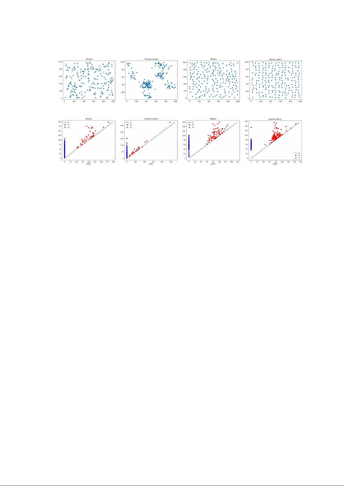
P ersistence Spheres: a Bi-con tin uous Linear Represen tation of Measures for P artial Optimal T ransp ort Matteo P egoraro ∗ Marc h 17, 2026 Abstract W e impro v e and extend p ersistence spheres, in tro duced in Pegoraro (2026). P ersistence spheres map an in tegrable measure µ on the upp er half-plane, including p ersistence di- agrams (PDs) as counting measures, to a function S ( µ ) ∈ C ( S 2 ), and the map is stable with resp ect to 1-W asserstein partial transp ort distance POT 1 . Moreo ver, to the b est of our kno wledge, p ersistence spheres are the ﬁrst explicit represen tation used in topolog- ical mac hine learning for whic h contin uit y of the in verse on the image is established at ev ery compactly supp orted target. Recen t bounded-cardinality bi-Lipschitz em b edding results in partial transp ort spaces, despite being p o werful, are not given b y the kind of explicit summary map considered here. Our construction is ro oted in conv ex geometry: for positive measures, the deﬁning ReLU in tegral is the support function of the lift zonoid. Building on P egoraro (2026), we reﬁne the deﬁnition to b etter match the POT 1 deletion mec hanism, enco ding partial transport via a signed diagonal augmen tation. In particular, for in tegrable µ , the uniform norm b etw een S (0) and S ( µ ) dep ends only on the persis- tence of µ , without any need of ad-ho c re-weigh tings, reﬂecting optimal transp ort to the diagonal at persistence cost. This yields a parameter-free represen tation at the lev el of measures (up to numerical discretization), while accommo dating future extensions where µ is a smo othed measure deriv ed from PDs (e.g., persistence in tensit y functions (W u et al., 2024)). Across clustering, regression, and classiﬁcation tasks inv olving functional data, time series, graphs, meshes, and p oin t clouds, the up dated p ersistence spheres are com- p etitiv e and often impro ve up on persistence images, persistence landscap es, p ersistence splines, and sliced W asserstein k ernel baselines. Keyw ords: lift zonoid, p ersistence diagrams, v ectorization, top ological machine learn- ing 1. In tro duction T opological Data Analysis (TD A) pro vides geometric descriptors designed to capture qual- itativ e structure in data while b eing robust to noise and, in man y contexts, insensitiv e to parametrization. Its ﬂagship to ol, p ersistent homolo gy , tracks homological features across a scale parameter, recording when connected comp onen ts, loops, and higher-dimensional ca vities are created and later ﬁlled in. The resulting summaries are t ypically enco ded as p ersistenc e diagr ams (PDs) or barco des, which hav e become standard ob jec ts for ex- ploratory analysis and for building top ologically informed learning pip elines (Edelsbrunner and Harer, 2010; Oudot, 2015). Distances and the non-linear geometry of diagrams. F rom a statistical viewp oin t, PDs are most naturally compared by W asserstein-t yp e distances deﬁned through p artial optimal tr ansp ort (POT), where unmatched mass is optimally sen t to the diagonal (Div ol ∗ . Institute of Computing, F acult y of Informatics, Univ ersit´ a della Svizzera Italiana 1 and Lacom b e, 2021). These metrics are central to stabilit y results, but they endow the space of diagrams with a strongly non-linear geometry . As a consequence, even elemen- tary op erations, suc h as av eraging, regression, or principal comp onen t analysis, do not admit straigh tforward analogues. F or instance, av erages can b e formulated as W asser- stein barycen ters (Mileyk o et al., 2011), which can b e costly to approximate and ma y b e non-unique, complicating b oth computation and interpretation. T opological mac hine learning via vectorizations. A large bo dy of w ork therefore fo cuses on mapping PDs into linear spaces where classical statistical to ols apply . This line of research underpins top olo gic al machine le arning (P apamarkou et al., 2024), where v ectorized topological features and diﬀeren tiable top ological ob jectives are used in predic- tiv e tasks and representation learning (Mo or et al., 2020; W ayland et al., 2024). Existing approac hes include explicit em b eddings and feature maps, as w ell as kernel metho ds (Rein- inghaus et al., 2015; Kusano et al., 2018; Carriere et al., 2017). Among explicit embeddings, one ﬁnds constructions based on descriptive statistics (Asaad et al., 2022), algebraic or tropical coordinates (Kali ˇ snik, 2019; Mono d et al., 2019; Di F abio and F erri, 2015), and functional represen tations such as landscap es, images, and related summaries (Bubenik, 2015; Adams et al., 2017; Biscio and Møller, 2019; Dong et al., 2024; Goto v ac Doga ˇ s and Mandari ´ c, 2025), alongside other geometric encodings (Mitra and Virk, 2024). T o the b est of our knowledge, how ever, none of these explicit vectorizations comes with some con tinuit y statemen t for the in v erse map. By con trast, for kernel-induced Hilb ert em- b eddings, the sliced W asserstein construction yields such a bi-contin uity statement on b ounded-cardinalit y sub classes, as we recall b elo w. A t the same time, strong imp ossibility results show that one cannot hop e for a globally faithful linearization of the W asserstein geometry of PDs. F ollo wing the syn thesis in Mitra and Virk (2024), the picture can b e summarized as follo ws: (i) the space of diagrams with ﬁnitely many p oin ts do es not admit a bi-Lipsc hitz em b edding into any Hilbert space (Mitra and Virk, 2021); (ii) ev en restricting to at most n p oin ts, no bi-Lipsc hitz embedding in to an y ﬁnite-dimensional Euclidean space exists (Carri ` ere and Bauer, 2019); (iii) on suc h b ounded-cardinalit y classes, a bi-contin uous embedding into a Hilb ert space can b e ac hieved via the sliced W asserstein construction (Carriere et al., 2017); (iv) on at most n p oin ts one can also obtain coarse embeddings in to Hilb ert spaces (Mitra and Virk, 2021, 2024); and (v) more recently , bi-Lipschitz embeddings in to a Hilb ert space ha ve b een obtained for diagrams with at most n p oin ts (Bate and Garcia Pulido, 2024). Notably , among these results, Carriere et al. (2017); Mitra and Virk (2024) pro vide explicit geometric constructions. More precisely , Carriere et al. (2017) pro ve that the sliced W asse rstein distance itself is bi-Lipsc hitz equiv alen t to POT 1 under a uniform bound on the num ber of p oin ts, while for the RKHS distance induced b y the sliced W asserstein kernel the comparison with POT 1 is given through contin uous con trol functions on the same b ounded-cardinalit y classes. P ersistence spheres and bi-con tin uit y (P egoraro, 2026). In Pegoraro (2026) we in tro duced p ersistenc e spher es , a functional representation sending a p ersistence diagram to a real-v alued function on S 2 , with t wo complementary guarantees: Lipschitz stability with respect to POT 1 and con tinuit y of the in verse on the image. In this sense, persistence spheres pro vide a form of geometric faithfulness which, to the best of our knowledge, is not a v ailable for other explicit representations of p ersistence diagrams curren tly used in top ological mac hine learning. The construction is ro oted in the lift-zonoid representation 2 of a measure: for a p ositiv e integrable measure µ , the map v 7− → Z ReLU( ⟨ v , (1 , p ) ⟩ ) dµ ( p ) is the supp ort function of the lift zonoid Z µ (Koshev oy and Mosler, 1998; Hendrych and Nagy, 2022). Comparison with P egoraro (2026). Relative to Pegoraro (2026), w e strengthen the framew ork in four directions: 1. POT coherence without re-weigh ting. The reﬁned deﬁnition matches the POT 1 geometry of deletions: the uniform norm betw een S (0) and S ( µ ) dep ends only on the p ersistence of µ , reﬂecting that unmatc hed mass is optimally sen t to the diagonal at cost equal to its p ersistence (see Remark 1). As a consequence, the represen tation can b e deﬁned directly at the lev el of measures, without introducing reweigh ting sc hemes or tuning parameters (b ey ond n umerical choices suc h as the discretization grid used to ev aluate the functions). 2. A measure-theoretic form ulation. W e work with integrable measures on the upp er half-plane endow ed with POT 1 (Div ol and Lacom b e, 2021), cov ering classical PDs (as discrete measures) and extending seamlessly to smo oth summaries such as p ersistenc e intensity functions (W u et al., 2024). This uniﬁed setting is geared tow ard statistical mo deling of p ersistence ob jects, allowing one to treat discrete diagrams and smo othed/estimated representations within a single geometry . 3. A comparativ e analysis of top ological summaries. Bey ond introducing the revised p ersistence-sphere map, w e compare how several standard summaries, in- cluding p ersistence landscap es, p ersistence images, p ersistence splines, and sliced W asserstein constructions, deform the underlying POT 1 geometry . This highlights the sp eciﬁc geometric biases induced by diﬀerent v ectorizations and helps explain part of their empirical b eha vior in the sup ervised and unsup ervised exp erimen ts. 4. Impro v ed empirical p erformance. Comparing against full exp erimen tal suite of P egoraro (2026) with the reﬁned deﬁnition yields generally impro v ed results across the same case studies, while av oiding any ad-ho c rew eighting of p ersistence pairs. Outline. After this introduction, Section 2 recalls the conv ex-analytic background on supp ort functions and lift zonoids, and Section 3 develops the measure-theoretic setting, including integrable measures, partial optimal transp ort, and its comparison with ordi- nary optimal transport on cross-augmented measures. In Section 4 we review the classical lift-zonoid transform and its con tinuit y properties, and in Section 5 we introduce the new signed lift-zonoid formulation of persistence spheres, prov e injectivity , and analyze basic qualitativ e phenomena. The core bi-contin uit y theory is established in Section 6: we ﬁrst pro ve uniform stability with resp ect to POT 1 , then deriv e inv erse con tin uity , including a lo cal H¨ older-t yp e inv erse b ound on ﬁxed compact sets. W e then pass to Hilb ert-v alued form ulations in Section 7, where we obtain L 2 ( S 2 ) versions of the main contin uit y results and compare our regime with related Hilb ert em b eddings from the literature. Section 8 places the signed augmen tation strategy in a broader p erspective, discussing ho w it relates to other linear summaries and k ernel constructions, while Section 9 studies how diﬀerent summaries deform the POT 1 geometry in simple mo del cases. Finally , the empirical part ev aluates the revised construction on sup ervised b enc hmarks (Section 11) and unsup er- vised sim ulations (Section 10), b efore Section 12 concludes with implications, limitations, and directions for future work. 3 2. Con v ex Sets and Supp ort F unctions W e brieﬂy review the notation and concepts from con vex analysis and geometry that will b e used throughout. Standard references include Ro c k afellar (1997); Salinetti and W ets (1979). Deﬁnition 1 Given c onvex sets A, B ⊂ R 3 and a sc alar λ ≥ 0 , deﬁne A ⊕ B : = { a + b : a ∈ A, b ∈ B } , λA : = { λa : a ∈ A } . Deﬁnition 2 Given a c omp act c onvex set A ⊂ R 3 , its supp ort function is h A : R 3 → R , h A ( v ) : = max a ∈ A ⟨ v , a ⟩ . The restriction h A | S 2 determines h A (hence A ), and Mink owski operations are linearized b y support functions: h λ 1 A ⊕ λ 2 B = λ 1 h A + λ 2 h B ( λ 1 , λ 2 ≥ 0) . Deﬁnition 3 Given c omp act subsets A, B ⊂ Z , with ( Z, d Z ) a metric sp ac e, their Haus- dorﬀ distanc e is d H ( A, B ) : = max n sup a ∈ A d Z ( a, B ) , sup b ∈ B d Z ( b, A ) o . Prop osition 1 L et A, B ⊂ R 3 b e nonempty c omp act c onvex sets. Then d H ( A, B ) = ∥ h A − h B ∥ L ∞ ( S 2 ) = sup v ∈ S 2 | h A ( v ) − h B ( v ) | , wher e d H her e denotes the Hausdorﬀ distanc e induc e d by the Euclide an norm on R 3 . In p articular, the map A 7− → h A | S 2 is inje ctive. 3. In tegrable Measures and Partial Optimal T ransp ort F or r ≥ 0, denote B r : = { p ∈ R 2 : ∥ p ∥ 2 ≤ r } , B c r : = R 2 \ B r . W e will work with inte gr able measures and uniformly inte gr able sequences; see, e.g., Hendryc h and Nagy (2022). Deﬁnition 4 L et Z ⊂ R 2 b e a Bor el set. A p ositive Bor el me asur e µ on E is c al le d in tegrable if it is ﬁnite and Z Z ∥ p ∥ 2 dµ ( p ) < ∞ . If Z = X , we denote by M the set of inte gr able p ositive Bor el me asur es on X . A se quenc e of inte gr able me asur es { µ n } n ∈ N on Z is uniformly integrable if lim r →∞ sup n ∈ N Z Z ∩ B c r ∥ p ∥ 2 dµ n ( p ) = 0 . 4 Since R 2 is a lo cally compact P olish space, every ﬁnite Borel measure on R 2 is a Radon measure. In particular, every in tegrable measure (Deﬁnition 4) is Radon, hence the results of Divol and Lacombe (2021) apply throughout. T o compare measures w e use w eak and v ague conv ergence; see, e.g., Kallenberg (1997). Deﬁnition 5 A se quenc e of inte gr able me asur es { µ n } n ∈ N c onver ges weakly to µ , written µ n w − → µ , if Z R 2 f dµ n → Z R 2 f dµ for every c ontinuous b ounde d f : R 2 → R . It c onver ges v aguely to µ , written µ n v − → µ , if Z R 2 f dµ n → Z R 2 f dµ for every c ontinuous c omp actly supp orte d f : R 2 → R . 3.1 Measures and p ersistence W e adopt a measure-theoretic persp ective on p ersistence diagrams (PDs), follo wing Divol and Lacombe (2021). Set X : = R 2 x 0 . Then Z µ = n M i =1 c i [0 , (1 , p i )] ⊂ R 3 , and its supp ort function is h Z µ ( v ) = n X i =1 c i ReLU  ⟨ v , (1 , p i ) ⟩  . The lift-zonoid corresp ondence is esp ecially p o werful: the map µ 7→ Z µ is injective and enjo ys sharp con tinuit y prop erties. In particular, Hausdorﬀ conv ergence of lift zonoids is equiv alent to weak conv ergence together with uniform integrabilit y of the underlying measures. This “bi-contin uit y” principle is one of the central mechanisms in P egoraro (2026), since it allo ws one to pass bac k and forth b et w een measures, supp ort functions, and conv ex b o dies. Prop osition 4 (Con vergence of Lift Zonoids) L et µ b e an inte gr able me asur e on R 2 and let { µ n } n ∈ N b e a se quenc e of inte gr able me asur es. Then d H ( Z µ n , Z µ ) → 0 ⇐ ⇒ µ n w − → µ and { µ n } n ∈ N is uniformly inte gr able . The construction developed in the next section is inspired by this classical picture, but adapted to the partial-transp ort geometry of p ersistence diagrams. There, the natural ob ject is no longer a p ositiv e lift zonoid itself, but a linear ReLU transform applied to the signed augmentation that enco des transp ort to the diagonal. 10 Figure 1: Example of the lift zonoid construction for a discrete measure µ = P i c i δ p i . Each atom contributes the segmen t c i [0 , (1 , p i )] ⊂ R 3 , and Z µ is obtained as their Mink owski sum. 5. P ersistence Spheres via Signed Lift-Zonoid T ransforms W e now in tro duce the linear transform underlying the new persistence-sphere construction. Motiv ated b y Section 4, w e k eep the same ReLU integrand as in the lift-zonoid represen- tation, but use it in a purely linear wa y so as to accommodate the diagonal augmen tation naturally asso ciated with POT 1 . Deﬁnition 11 (Signed Lift-Zonoid T ransform) L et σ b e a ﬁnite signe d Bor el me a- sur e on R 2 such that Z R 2 ∥ (1 , p ) ∥ 2 d | σ | ( p ) < ∞ , wher e | σ | denotes the total variation me asur e. The signed lift-zonoid transform of σ is the function Λ( σ ) : R 3 → R , Λ( σ )( v ) : = Z R 2 ReLU  ⟨ v , (1 , p ) ⟩  dσ ( p ) . Prop osition 5 F or σ 1 , σ 2 satisfying Deﬁnition 11 and λ 1 , λ 2 ∈ R , Λ( λ 1 σ 1 + λ 2 σ 2 ) = λ 1 Λ( σ 1 ) + λ 2 Λ( σ 2 ) . F or p ositiv e in tegrable measures, this reduces exactly to the support-function represen- tation of Deﬁnition 10. Thus the signed transform should b e viewed as a linear extension of the classical lift-zonoid formula rather than as a diﬀeren t construction. W e deﬁne persistence spheres from measures on the upper half-plane X b y augmentin g eac h measure through its diagonal pro jection π ∆ . 11 Deﬁnition 12 (Augmented Measure) L et µ b e a p ositive Bor el me asur e on X . We deﬁne its augmen ted measure as the signe d me asur e on X µ aug : = µ − ( π ∆ ) # µ. Prop osition 6 L et µ ∈ M . Then µ aug satisﬁes the inte gr ability c ondition of Deﬁni- tion 11, and ther efor e Λ( µ aug ) is wel l deﬁne d. Pro of Using (1) with f = π ∆ : X → ∆ and g ( z ) = ∥ (1 , z ) ∥ 2 , the inequalit y ∥ π ∆ ( p ) ∥ 2 ≤ ∥ p ∥ 2 giv es Z ∆ ∥ (1 , z ) ∥ 2 d ( π ∆ ) # µ ( z ) = Z X ∥ (1 , π ∆ ( p )) ∥ 2 dµ ( p ) ≤ Z X ∥ (1 , p ) ∥ 2 dµ ( p ) < ∞ . Hence Z X ∥ (1 , u ) ∥ 2 d | µ aug | ( u ) ≤ Z X ∥ (1 , p ) ∥ 2 dµ ( p ) + Z ∆ ∥ (1 , z ) ∥ 2 d ( π ∆ ) # µ ( z ) < ∞ , so µ aug satisﬁes Deﬁnition 11. Deﬁnition 13 (Persistence sphere) F or µ ∈ M , the p ersistence sphere of µ is the r estriction to S 2 of the signe d lift-zonoid tr ansform of its augmentation: S ( µ ) : S 2 → R , S ( µ ) : =  Λ( µ aug )    S 2 . W e no w relate diﬀerences of p ersistence spheres to cross-augmen tation. Given µ, ν ∈ M , recall µ ⊕ ∆ ν = µ + ( π ∆ ) # ν from (2). A direct computation yields the identit y of signed measures on X , µ aug − ν aug = ( µ ⊕ ∆ ν ) − ( ν ⊕ ∆ µ ) . (3) By linearity of Λ (Prop osition 5), restricting to S 2 giv es S ( µ ) − S ( ν ) =  Λ( µ ⊕ ∆ ν ) − Λ( ν ⊕ ∆ µ )     S 2 . (4) Consequen tly , for an y norm ∥ · ∥ on a function space ov er S 2 (e.g. L p ( S 2 ) or L ∞ ( S 2 )), ∥ S ( µ ) − S ( ν ) ∥ =     Λ( µ ⊕ ∆ ν ) − Λ( ν ⊕ ∆ µ )     S 2    . (5) Note that the measures µ ⊕ ∆ ν and ν ⊕ ∆ µ are p ositiv e b y construction. Moreov er, they are integrable on X by Prop osition 2. Thus, although p ersistence spheres are deﬁned through an augmented signed measure, their diﬀerences can b e expressed in terms of p ositiv e cross-augmented measures, which will allow us to reco ver injectivit y and con tinuit y prop erties b y comparison with the classical lift-zonoid setting. The p ersistence-sphere construction here diﬀers substan tially from the one in Pegoraro (2026). There, one ﬁrst reweigh ts the diagram measure through a p ersistence-dep enden t sc heme with additional dep endence on ∥ p ∥ 2 , and then applies the lift-zonoid transform, so that the resulting function is directly the supp ort function of a lift zonoid. In contrast, we a void rew eighting altogether and enco de deletions through diagonal augmen tation, yielding a parameter-free deﬁnition at the level of measures (up to numerical ev aluation c hoices). As a ﬁrst step, we obtain injectivity of the nov el representation. 12 Prop osition 7 L et µ, ν ∈ M . If S ( µ ) = S ( ν ) , then µ = ν . Pro of By Equation (5), S ( µ ) = S ( ν ) implies Λ( µ ⊕ ∆ ν ) = Λ( ν ⊕ ∆ µ ), and injectivit y of the lift-zonoid transform on integrable measures (Koshev oy and Mosler, 1998; Hendryc h and Nagy, 2022), in turn, giv es µ ⊕ ∆ ν = ν ⊕ ∆ µ as p ositiv e measures on X . Th us, µ − ν = ( π ∆ ) # ( ν − µ ). As the measures on the tw o sides of the equality ha ve disjoint supp orts, they must be zero for every measurable set. 5.1 A Con v enien t Change of Coordinates With the p ersistence-sphere map no w in place, w e next in tro duce a change of co ordinates adapted to the structure of POT. This reformulation is not essential for the deﬁnition itself, but it simpliﬁes the expressions app earing b elo w and clariﬁes the geometric role of p ersistence. W e w ant to separate diagonal and oﬀ–diagonal v ariability . F or v = ( v 0 , v 1 , v 2 ) ∈ S 2 deﬁne s ( v ) := v 1 + v 2 , t ( v ) := v 2 − v 1 , (6) whic h represent, resp ectiv ely , the components of ( v 1 , v 2 ) along (1 , 1) (diagonal direction) and ( − 1 , 1) (oﬀ–diagonal direction). F or p = ( x, y ) ∈ X recall that d ( p ) = x + y 2 , Pers( p ) = y − x 2 , (7) so that d is the co ordinate along the diagonal and P ers is the distance to the diagonal (p ersistence). With this notation, the ReLU arguments app earing in the deﬁnition of p ersistence spheres decomp ose as ⟨ v , (1 , p ) ⟩ = v 0 + s ( v ) d ( p ) + t ( v ) P ers( p ) , ⟨ v , (1 , π ∆ ( p )) ⟩ = v 0 + s ( v ) d ( p ) . (8) In particular, the p oin t wise in tegrand in the deﬁnition of S is ϕ v ( p ) : = ReLU  v 0 + d ( p ) s ( v ) + P ers( p ) t ( v )  − ReLU  v 0 + d ( p ) s ( v )  . (9) Equation (8) will b e used rep eatedly in the up coming pro ofs, since it makes explicit ho w directions v prob e diagonal lo cation ( s ( v )) and ho w they prob e p ersistence ( t ( v )). It also mak es transparen t an imp ortan t qualitative feature of p ersistence spheres: under large one-sided translations along the diagonal, the represen tation ev en tually forgets the exact d -lo cation and retains only the p ersistence con tribution, as the tw o d -contributions delete each other. Lastly we recall that ReLU is 1-Lipschitz: | ReLU( a ) − ReLU( b ) | ≤ | a − b | ∀ a, b ∈ R . (10) Prop osition 8 (Diagonal drifts) L et { µ n } ⊂ M b e a se quenc e of inte gr able me asur es and assume ther e exists M < ∞ such that sup n sup p ∈ supp( µ n ) P ers( p ) ≤ M . (11) (A + ) Drift to + ∞ along the diagonal. Assume ∀ R > 0 , µ n  { d ≤ R }  − → 0 . (12) 13 Then for every ﬁxe d v ∈ S 2 with s ( v )  = 0 , S ( µ n )( v ) − 1 { s ( v ) > 0 } t ( v ) Pers( µ n ) − → 0 . (13) In p articular, if P ers( µ n ) → P ∈ [0 , ∞ ) , then for every such v , S ( µ n )( v ) − → ( 0 , s ( v ) < 0 , t ( v ) P , s ( v ) > 0 . (A − ) Drift to −∞ along the diagonal. Assume ∀ R > 0 , µ n  { d ≥ − R }  − → 0 . (14) Then for every ﬁxe d v ∈ S 2 with s ( v )  = 0 , S ( µ n )( v ) − 1 { s ( v ) < 0 } t ( v ) Pers( µ n ) − → 0 . (15) In p articular, if P ers( µ n ) → P ∈ [0 , ∞ ) , then for every such v , S ( µ n )( v ) − → ( t ( v ) P , s ( v ) < 0 , 0 , s ( v ) > 0 . Pro of W e prov e (A + ); the proof of (A − ) is analogous. Fix v ∈ S 2 with s ( v )  = 0, and abbreviate s := s ( v ) , t := t ( v ) . W e c ho ose R v := | v 0 | + | t | M + 1 | s | so that, whenev er d ( p ) ≥ R v , one has | s | d ( p ) ≥ | v 0 | + | t | M + 1 . Let now p ∈ X satisfy d ( p ) ≥ R v and supp ose s > 0. Recall that Equation (8), ⟨ v , (1 , π ∆ ( p )) ⟩ = v 0 + s d ( p ) , ⟨ v , (1 , p ) ⟩ = v 0 + s d ( p ) + t Pers( p ) . Since d ( p ) ≥ R v , we ha ve s d ( p ) ≥ sR v = | v 0 | + | t | M + 1 . Therefore ⟨ v , (1 , π ∆ ( p )) ⟩ = v 0 + s d ( p ) ≥ v 0 + sR v ≥ | t | M + 1 > 0 , and, using also P ers( p ) ≤ M , ⟨ v , (1 , p ) ⟩ = v 0 + s d ( p ) + t Pers( p ) ≥ v 0 + sR v − | t | Pers( p ) ≥ v 0 + sR v − | t | M ≥ 1 > 0 . Hence b oth ReLU arguments are p ositiv e and therefore ϕ v ( p ) = ⟨ v , (1 , p ) ⟩ − ⟨ v , (1 , π ∆ ( p )) ⟩ = t P ers( p ) . 14 If instead s < 0, then again using (11), ⟨ v , (1 , π ∆ ( p )) ⟩ = v 0 + s d ( p ) ≤ v 0 + sR v < −| t | M − 1 < 0 , and ⟨ v , (1 , p ) ⟩ = v 0 + s d ( p ) + t Pers( p ) ≤ v 0 + sR v + | t | M ≤ − 1 < 0 . Hence b oth ReLU arguments are negative and therefore ϕ v ( p ) = 0 . Th us, for ev ery p with d ( p ) ≥ R v , ϕ v ( p ) = 1 { s> 0 } t Pers( p ) . It follows that S ( µ n )( v ) − 1 { s> 0 } t Pers( µ n ) = Z { d 0 } t Pers( p )  dµ n ( p ) . Using (9) and the 1-Lipsc hitz prop ert y of ReLU, | ϕ v ( p ) | ≤ | t | P ers( p ) ≤ | t | M , hence    ϕ v ( p ) − 1 { s> 0 } t Pers( p )    ≤ 2 | t | M for all p ∈ X. Therefore   S ( µ n )( v ) − 1 { s> 0 } t Pers( µ n )   ≤ 2 | t | M µ n ( { d < R v } ) . Since (12) holds for every R > 0, in particular for R = R v , the righ t-hand side tends to 0. This prov es (13). The ﬁnal con vergence statemen t follows immediately if P ers( µ n ) → P . The pro of of (A − ) is iden tical, exchanging the roles of the tw o tails. Moreo ver, for every µ , the p ersistence sphere S ( µ ) satisﬁes a sign constraint on the region { t ( v ) < 0 } = { v 1 > v 2 } . Lemma 1 (A general sign constrain t) L et µ ∈ M . Then for every v ∈ S 2 such that t ( v ) ≤ 0 , S ( µ )( v ) ≤ 0 . Pro of By Equation (9), if t ( v ) ≤ 0 then for every p ∈ X the ﬁrst ReLU argument is b ounded ab o v e by the second one. Hence ϕ v ( p ) ≤ 0 ∀ p ∈ X , and therefore S ( µ )( v ) = Z X ϕ v ( p ) dµ ( p ) ≤ 0 . Prop osition 8 mak es precise a ﬂattening phenomenon for p ersistence spheres under one-sided diagonal drift. Under a uniform b ound on p ersistence, the sign of the ReLU argumen ts in Equation (8) stabilizes for every ﬁxed direction with s ( v )  = 0, and the sphere 15 v alues even tually dep end only on the total p ersistence. In this regime, diﬀerences purely in the diagonal co ordinate d are asymptotically erased: once mass is translated far enough along (1 , 1) in one direction, the representation retains only whether the c hosen direction detects that tail, and, if so, through the scalar factor t ( v ) Pers( µ n ). The counting-measure case is made explicit in Corollary 1. This should not b e viewed as an isolated pathology of p ersistence spheres. Rather, some form of ﬂattening or geometric compression appears to b e unav oidable for every linearization of p ersistence diagrams: an y passage to a linear space necessarily distorts part of the original partial-transp ort geometry . What is sp eciﬁc to persistence spheres is the particularly transparent form that this eﬀect takes under diagonal drift, whic h can b e describ ed explicitly in terms of the co ordinates s ( v ) and t ( v ). W e return to this broader theme in Section 9, where p ersistence spheres are compared with other standard summaries from this viewpoint. By con trast, Lemma 1 is a general one-sided fact: directions with t ( v ) ≤ 0 alw ays yield a nonp ositiv e con tribution, indep enden tly of an y asymptotic regime. A k ey observ ation is that the p oin twise limits arising in Prop osition 8 are discon tin uous on S 2 : for drift to + ∞ , the limiting function is v 7− → 1 { s ( v ) > 0 } t ( v ) P , and for drift to −∞ it is v 7− → 1 { s ( v ) < 0 } t ( v ) P , with jumps across the great circle { s ( v ) = 0 } . Consequen tly , such diagonal-drift regimes cannot o ccur along a sequence for which p ersistence spheres con verge uniformly on S 2 , since uniform limits of con tin uous functions are con tinuous. This observ ation helps explain wh y large one-sided diagonal drift must be excluded, or quan titatively con trolled, in the uniform inv erse-con tinuit y arguments developed later. Corollary 1 L et { p 1 , . . . , p N } b e a ﬁnite set and µ = P N i =1 δ p i . Deﬁne µ k := P N i =1 δ p i +( k,k ) . Then for every v ∈ S 2 with s ( v )  = 0 , lim k →∞ S ( µ k )( v ) = ( 0 , s ( v ) < 0 , t ( v ) Pers( µ ) , s ( v ) > 0 . The next lemma quantiﬁes, in a particularly simple one-point setting, how quickly the diagonal-coordinate v ariabilit y is w ashed out b y large translations along (1 , 1). More precisely , if tw o one-p oin t diagrams diﬀer only b y a ﬁxed oﬀset in the d -direction and are b oth shifted by ( k, k ), then the corresponding persistence spheres b ecome ev en tually iden tical in eac h ﬁxed direction v , and their uniform discrepancy decays at worst like O (1 /k ). In this sense, the lemma provi des a quantitativ e companion to the p oin twise asymptotics of Proposition 8 and corollary 1. Lemma 2 Fix p ∈ X and set d := d ( p ) and P := Pers( p ) > 0 . L et h > 0 b e ﬁxe d and, for k ≥ 1 , deﬁne µ k := δ p +( k,k ) , ν k := δ p +( k + h,k + h ) . Then for every k ≥ | d | + 2 h ,   S ( µ k ) − S ( ν k )   ∞ ≤ 2 h  1 + √ 2 P  k . (16) 16 Pro of Fix v ∈ S 2 and abbreviate s := s ( v ) and t := t ( v ). Set K := t P , a k := v 0 + s ( d + k ) , F K ( a ) := ReLU( a + K ) − ReLU( a ) , so that S ( µ k )( v ) = F K ( a k ) , S ( ν k )( v ) = F K ( a k + hs ) , Γ k ( v ) = F K ( a k ) − F K ( a k + hs ) . Since F K is 1–Lipschitz, | Γ k ( v ) | ≤ h | s | . (17) F or (16), note that F K has breakp oin ts at a = 0 and a = − K , hence it is constant (with v alue either 0 or K ) outside the interv al J K :=  min {− K, 0 } , max {− K, 0 }  ⊂ [ −| K | , | K | ] . Therefore, if Γ k ( v )  = 0, the segmen t [ a k , a k + hs ] in tersects J K , so there exists λ ∈ [0 , 1] suc h that z := a k + λhs ∈ J K ⊂ [ −| K | , | K | ] . Hence | a k | ≤ | a k − z | + | z | ≤ λh | s | + | K | ≤ h | s | + | K | , and so | a k | ≤ | K | + h | s | . (18) On the other hand, | a k | = | v 0 + s ( d + k ) | ≥ | s | | d + k | − | v 0 | ≥ | s | ( k − | d | ) − 1 . Com bining with (18) gives, whenev er Γ k ( v )  = 0, | s | ( k − | d | ) − 1 ≤ | K | + h | s | = ⇒ ( k − | d | − h ) | s | ≤ 1 + | K | . If k ≥ | d | + 2 h , then k − | d | − h ≥ k / 2, so | s | ≤ 2(1 + | K | ) k . Plugging into (17) yields | Γ k ( v ) | ≤ h | s | ≤ 2 h (1 + | K | ) k . Finally , | K | = | t | P ≤ √ 2 P since | t ( v ) | ≤ ∥ ( v 1 , v 2 ) ∥ 1 ≤ √ 2, so | Γ k ( v ) | ≤ 2 h (1 + √ 2 P ) k . 6. Uniform Conv ergence Results As suggested by Prop osition 1, the most natural metric to emplo y to compare p ersistence spheres is the sup norm. Th us we start obtaining bi-con tinuit y results relying on such norm, even if it do es not meet our ﬁnal goal of embedding measures in a Hilbert space. 17 6.1 Stabilit y In this section w e establish the forward con tinuit y direction (stability) of p ersistence spheres: closeness in POT 1 implies uniform closeness of the asso ciated sphere functions. The key p oint is that S ( µ ) is built from a ReLU transform, so the diﬀerence S ( µ ) − S ( ν ) can b e rewritten as the action of a ﬁxed Lipschitz test family on t wo cross-augmen ted measures. This brings the problem in to the scop e of Kantoro vic h–Rubinstein duality for OT 1 , and yields a global Lipschitz b ound ∥ S ( µ ) − S ( ν ) ∥ ∞ ≲ POT 1 ( µ, ν ) (Theorem 2). W e also emphasize that this choice of metric is essen tially forced: as shown in Skraba and T urner (2020) in the broader setting of W asserstein-stable linear representations of p ersistence diagrams, one cannot exp ect stabilit y for linear op erators on diagram measures with resp ect to other W asserstein distances. Theorem 2 ( POT 1 Con v ergence ⇒ Uniform Spheres) F or al l µ, ν ∈ M , ∥ S ( µ ) − S ( ν ) ∥ ∞ ≤ 2 √ 2 POT 1 ( µ, ν ) . Pro of Recall the cross-augmen tation identit y (3): µ aug − ν aug = ( µ ⊕ ∆ ν ) − ( ν ⊕ ∆ µ ) , hence by linearit y of Λ (Prop osition 5), S ( µ ) − S ( ν ) =  Λ( µ ⊕ ∆ ν ) − Λ( ν ⊕ ∆ µ )     S 2 . (19) Step 1: a Lipschitz test family . F or v ∈ S 2 , deﬁne ψ v : X → R b y ψ v ( u ) : = ReLU  ⟨ v , (1 , u ) ⟩  . Note that ∥ ( v 1 , v 2 ) ∥ 1 ≤ √ 2 for all v = ( v 0 , v 1 , v 2 ) ∈ S 2 . (20) Then ψ v is √ 2-Lipsc hitz on ( X , ∥ · ∥ ∞ ). Indeed, using | ReLU( a ) − ReLU( b ) | ≤ | a − b | and (20), for u, w ∈ X , | ψ v ( u ) − ψ v ( w ) | ≤ |⟨ v , (1 , u ) ⟩−⟨ v , (1 , w ) ⟩| = |⟨ ( v 1 , v 2 ) , u − w ⟩| ≤ ∥ ( v 1 , v 2 ) ∥ 1 ∥ u − w ∥ ∞ ≤ √ 2 ∥ u − w ∥ ∞ . Step 2: Kantoro vic h–Rubinstein dualit y for OT 1 . Using the dual formulation of OT 1 (Kan torovic h–Rubinstein), OT 1 ( ˜ µ, ˜ ν ) = sup Lip( f ) ≤ 1 Z X f d ( ˜ µ − ˜ ν ) , where Lip( f ) ≤ 1 is with resp ect to ∥ · ∥ ∞ on X . Apply this with ˜ µ = µ ⊕ ∆ ν and ˜ ν = ν ⊕ ∆ µ . Since each ψ v is √ 2-Lipsc hitz, w e obtain for ev ery v ∈ S 2 :   Λ( µ ⊕ ∆ ν )( v ) − Λ( ν ⊕ ∆ µ )( v )   =     Z X ψ v ( u ) d  ( µ ⊕ ∆ ν ) − ( ν ⊕ ∆ µ )  ( u )     ≤ √ 2 OT 1 ( µ ⊕ ∆ ν, ν ⊕ ∆ µ ) . T aking the supremum o ver v ∈ S 2 and using (19) gives ∥ S ( µ ) − S ( ν ) ∥ ∞ ≤ √ 2 OT 1 ( µ ⊕ ∆ ν, ν ⊕ ∆ µ ) . Finally , Prop osition 3 yields OT 1 ( µ ⊕ ∆ ν, ν ⊕ ∆ µ ) ≤ 2 POT 1 ( µ, ν ) , whic h concludes the pro of. 18 6.2 In v erse Con tinuit y The proof of in verse con tinuit y is more delicate, holds only for con vergence to compactly supp orted measures, and is organized in to sev eral steps. W e b egin b y testing persistence spheres in suitable directions, whic h allows us to detect geometric regimes implied b y uniform conv ergence. W e then prov e a lo cal inv erse estimate for measures supported on a ﬁxed compact set. These ingredients are ﬁnally assembled to derive the global in verse- con tinuit y result. 6.2.1 Test Directions The inv erse-contin uit y argumen t relies on a small set of directions v ∈ S 2 for which ϕ v has a simple form, so that S ( µ )( v ) directly con trols sp eciﬁc p ortions of µ . W e start with tw o basic estimates: one reads oﬀ total persistence from a single direction, and the other quantiﬁes ho w muc h S ( η ) changes when η is truncated to a measurable subset. W e then construct tw o families of directions: one detecting mass far out in the d -direction (Lemma 5), and one detecting b oth low- and high-p ersistence contributions (Lemma 6). Lemma 3 (T otal Persistence) L et v Pers = (0 , − 1 / √ 2 , 1 / √ 2) ∈ S 2 . Then for every µ ∈ M , S ( µ )( v Pers ) = √ 2 Pers( µ ) , henc e Pers( µ ) = 1 √ 2 S ( µ )( v Pers ) . Conse quently, if ∥ S ( µ n ) − S ( µ ) ∥ ∞ → 0 , then Pers( µ n ) → P ers( µ ) and sup n P ers( µ n ) < ∞ . Pro of Let p = ( x, y ) ∈ X . F or v Pers = (0 , − 1 / √ 2 , 1 / √ 2) we ha ve s ( v Pers ) = 0 , t ( v Pers ) = √ 2 . Therefore, by Equation (8), ⟨ v Pers , (1 , p ) ⟩ = √ 2 Pers( p ) , ⟨ v Pers , (1 , π ∆ ( p )) ⟩ = 0 . Since Pers( p ) > 0 on X , b oth argumen ts of ReLU are nonnegative, hence Equation (9) yields ϕ v Pers ( p ) = √ 2 Pers( p ) . In tegrating against µ gives S ( µ )( v Pers ) = √ 2 Pers( µ ), and the remaining claims follow immediately . Lemma 4 (T runcation) F or any η ∈ M and any me asur able A ⊂ X , ∥ S ( η ) − S ( η | A ) ∥ ∞ ≤ √ 2 Z A c P ers( p ) dη ( p ) . Pro of Fix v ∈ S 2 and p ∈ X . By Equation (9) and the 1-Lipschitz prop ert y Equation (10), | ϕ v ( p ) | ≤   P ers( p ) t ( v )   ≤ | t ( v ) | P ers( p ) ≤ ∥ ( v 1 , v 2 ) ∥ 1 P ers( p ) ≤ √ 2 Pers( p ) , where we used | t ( v ) | = | v 2 − v 1 | ≤ | v 1 | + | v 2 | = ∥ ( v 1 , v 2 ) ∥ 1 and Equation (20). Therefore, | S ( η )( v ) − S ( η | A )( v ) | =    Z A c ϕ v ( p ) dη ( p )    ≤ √ 2 Z A c P ers( p ) dη ( p ) , and taking the suprem um o v er v ∈ S 2 giv es the claim. 19 Remark 1 A p articularly simple instanc e of p artial tr ansp ort is tr ansp ort to the nul l me a- sur e. Sinc e the only p artial plan fr om η | A to 0 is the zer o plan, al l mass is left unmatche d and ther efor e sent to the diagonal. Henc e, for every η ∈ M and every me asur able A ⊂ X , POT 1 ( η | A , 0) = Z A P ers( p ) dη ( p ) . In the same spirit, c ombining Lemma 3 with Lemma 4 yields an exact formula for the distanc e fr om the nul l p ersistenc e spher e: ∥ S ( µ ) − S (0) ∥ ∞ = √ 2 Pers( µ ) , µ ∈ M . Inde e d, Lemma 3 gives the lower b ound ∥ S ( µ ) ∥ ∞ ≥ S ( µ )( v Pers ) = √ 2 Pers( µ ) , while Lemma 4, applie d with A = ∅ , gives the matching upp er b ound ∥ S ( µ ) − S (0) ∥ ∞ ≤ √ 2 Pers( µ ) . Thus the uniform distanc e fr om S (0) is determine d exactly by the total p ersistenc e of µ . The next lemma constructs, for a compactly supp orted measure µ , a direction v ∈ S 2 that kills the con tribution of the ﬁxed compact supp ort supp µ and isolates p ersistence mass escaping far a wa y in the d -co ordinate. Indeed, using Equation (8), we choose v 0 < 0 and small positive co eﬃcien ts s ( v ) , t ( v ) so that b oth ReLU argumen ts are nonp ositiv e on supp µ , hence S ( µ )( v ) = 0. On the other hand, once d ( p ) is large enough, the term v 0 + s ( v ) d ( p ) b ecomes p ositive; in that regime b oth ReLU argumen ts are active and their diﬀerence is exactly t ( v ) P ers( p ). The direction v th us suppresses the compact core and detects only persistence mass drifting to + ∞ along the d -axis. Lemma 5 (F ar Awa y) L et µ ∈ M have c omp act supp ort in X . Cho ose R 0 , M 0 > 0 such that supp µ ⊂  p ∈ X : | d ( p ) | ≤ R 0 and Pers( p ) ≤ M 0  . Set s 0 := 1 2 R 0 , t 0 := 1 2 M 0 , ˜ v :=  − 1 , s 0 − t 0 2 , s 0 + t 0 2  ∈ R 3 , v := ˜ v ∥ ˜ v ∥ 2 ∈ S 2 . Then: 1. s ( v ) > 0 and t ( v ) > 0 . 2. F or every p ∈ supp µ , ⟨ v , (1 , p ) ⟩ ≤ 0 and ⟨ v, (1 , π ∆ ( p )) ⟩ < 0 , henc e S ( µ )( v ) = 0 . 3. Ther e exists R ∗ ( µ ) > 0 such that for every p ∈ X with d ( p ) ≥ R ∗ , ϕ v ( p ) = ReLU( ⟨ v , (1 , p ) ⟩ ) − ReLU( ⟨ v , (1 , π ∆ ( p )) ⟩ ) = P ers( p ) t ( v ) . 20 Pro of (1) By construction, s ( ˜ v ) = ( ˜ v ) 1 + ( ˜ v ) 2 = s 0 > 0 , t ( ˜ v ) = ( ˜ v ) 2 − ( ˜ v ) 1 = t 0 > 0 . Normalization by the p ositiv e scalar ∥ ˜ v ∥ 2 preserv es signs, hence s ( v ) > 0 and t ( v ) > 0. (2) Fix p ∈ supp µ . Then | d ( p ) | ≤ R 0 and P ers( p ) ≤ M 0 . Using Equation (8) with v = ˜ v giv es ⟨ ˜ v , (1 , p ) ⟩ = − 1 + d ( p ) s ( ˜ v ) + Pers( p ) t ( ˜ v ) , ⟨ ˜ v , (1 , π ∆ ( p )) ⟩ = − 1 + d ( p ) s ( ˜ v ) . Since s ( ˜ v ) = s 0 and t ( ˜ v ) = t 0 , we ha ve | d ( p ) s ( ˜ v ) | ≤ R 0 s 0 = 1 2 , | Pers( p ) t ( ˜ v ) | ≤ M 0 t 0 = 1 2 , hence ⟨ ˜ v , (1 , p ) ⟩ ≤ − 1 + 1 2 + 1 2 = 0 , ⟨ ˜ v , (1 , π ∆ ( p )) ⟩ ≤ − 1 + 1 2 = − 1 2 < 0 . After normalization the inequalities preserv e sign, so the same b ounds hold for v . In particular, ReLU( ⟨ v , (1 , p ) ⟩ ) = 0 and ReLU( ⟨ v , (1 , π ∆ ( p )) ⟩ ) = 0 for all p ∈ supp µ , hence ϕ v ( p ) = 0 on supp µ by Equation (9). Integrating against µ yields S ( µ )( v ) = 0. (3) By Equation (8), ⟨ v , (1 , π ∆ ( p )) ⟩ = v 0 + d ( p ) s ( v ) . Since s ( v ) > 0 b y (1), this quan tity tends to + ∞ as d ( p ) → + ∞ . Th us there exists R ∗ ( µ ) > 0 suc h that for all p with d ( p ) ≥ R ∗ ( µ ), ⟨ v , (1 , π ∆ ( p )) ⟩ > 0 . Moreo ver, ⟨ v , (1 , p ) ⟩ = ⟨ v , (1 , π ∆ ( p )) ⟩ + P ers( p ) t ( v ) ≥ ⟨ v , (1 , π ∆ ( p )) ⟩ > 0 , since Pers( p ) ≥ 0 and t ( v ) > 0. Hence on { d ≥ R ∗ ( µ ) } b oth ReLU arguments are p ositiv e, and therefore ϕ v ( p ) = ⟨ v , (1 , p ) ⟩ − ⟨ v , (1 , π ∆ ( p )) ⟩ = P ers( p ) t ( v ) . Remark 2 ( d → −∞ ) Deﬁne R : R 3 → R 3 by R ( v 0 , v 1 , v 2 ) := ( v 0 , − v 2 , − v 1 ) . Then s ( R v ) = − s ( v ) and t ( R v ) = t ( v ) , and ⟨R v , (1 , p ) ⟩ = v 0 + ( − d ( p )) s ( v ) + P ers( p ) t ( v ) . In p articular, if v is given by Lemma 5, then R v satisﬁes the analo gue of Lemma 5(2)–(3) on the d → −∞ side: S ( µ )( R v ) = 0 , and ther e exists R ′ ∗ ( µ ) > 0 such that for d ( p ) ≤ − R ′ ∗ , ϕ R v ( p ) = P ers( p ) t ( v ) . 21 The next lemma in tro duces a second family of test directions, this time aimed at probing persistence levels indep enden tly of the diagonal coordinate. In contrast with the previous construction, we no w imp ose s ( v ) = 0, so that the ReLU arguments no longer dep end on d ( p ) and are controlled only by P ers( p ). By choosing the remaining parameters appropriately , one obtains directions v δ for which the in tegrand v anishes below a prescrib ed p ersistence threshold δ and gro ws linearly ab o v e it, namely as t δ (P ers − δ ) + . In this wa y , sphere ev aluations in these directions isolate the contribution of the high- p ersistence tail, while suitable com binations also control the mass concentrated at lo w p ersistence. Lemma 6 (Low and High P ersistence) F or δ ≥ 0 deﬁne t δ := r 2 1 + 2 δ 2 , v δ :=  − δ t δ , − t δ 2 , t δ 2  ∈ S 2 . Then for every η ∈ M and every δ ≥ 0 , S ( η )( v δ ) = t δ Z X (P ers − δ ) + dη , (21) Z { Pers ≥ 2 δ } P ers dη ≤ 2 Z X (P ers − δ ) + dη = 2 t δ S ( η )( v δ ) , (22) and Z { Pers <δ } P ers dη ≤ Z X g δ (P ers) dη = 1 √ 2 S ( η )( v 0 ) − 2 1 t δ S ( η )( v δ ) + 1 t 2 δ S ( η )( v 2 δ ) , (23) wher e g δ ( r ) := r − 2( r − δ ) + + ( r − 2 δ ) + , r ≥ 0 . Pro of By construction s ( v δ ) = v δ, 1 + v δ, 2 = 0 , t ( v δ ) = v δ, 2 − v δ, 1 = t δ > 0 . Hence for ev ery p ∈ X , ⟨ v δ , (1 , p ) ⟩ = v δ, 0 + t δ P ers( p ) , ⟨ v δ , (1 , π ∆ ( p )) ⟩ = v δ, 0 . Since v δ, 0 = − δ t δ ≤ 0, w e ha v e ReLU( v δ, 0 ) = 0, and therefore Equation (9) yields ϕ v δ ( p ) = ReLU  v δ, 0 + t δ P ers( p )  − ReLU( v δ, 0 ) = ReLU  t δ (P ers( p ) − δ )  = t δ (P ers( p ) − δ ) + . In tegrating against η giv es Equation (21). F or δ = 0 one has v 0 = v Pers and t 0 = √ 2, so Equation (21) reduces to S ( η )( v 0 ) = √ 2 R X P ers dη , consisten t with Lemma 3. F or an y r ≥ 0, r 1 { r ≥ 2 δ } ≤ 2( r − δ ) + . Indeed, if r < 2 δ the left-hand side is 0, while if r ≥ 2 δ then ( r − δ ) + = r − δ ≥ r / 2, i.e. r ≤ 2( r − δ ) + . Applying this inequalit y with r = Pers( p ) and in tegrating yields Z { Pers ≥ 2 δ } P ers dη ≤ 2 Z X (P ers − δ ) + dη , 22 and the ﬁnal iden tity in Equation (22) follo ws from Equation (21). Deﬁne g δ ( r ) := r − 2( r − δ ) + + ( r − 2 δ ) + , r ≥ 0 . A direct c hec k giv es g δ ( r ) =      r , 0 ≤ r ≤ δ , 2 δ − r, δ ≤ r ≤ 2 δ, 0 , r ≥ 2 δ, hence g δ ( r ) ≥ r 1 { r<δ } . Therefore, Z { Pers <δ } P ers dη ≤ Z X g δ (P ers) dη . Finally , expanding g δ and using Equation (21) with parameters 0, δ , and 2 δ yields Z X g δ (P ers) dη = Z X P ers dη − 2 Z X (P ers − δ ) + dη + Z X (P ers − 2 δ ) + dη = 1 √ 2 S ( η )( v 0 ) − 2 1 t δ S ( η )( v δ ) + 1 t 2 δ S ( η )( v 2 δ ) , where w e also used Lemma 3 to rewrite R X P ers dη = 1 √ 2 S ( η )( v 0 ). This prov es Equa- tion (23). 6.2.2 V anishing of the T ails W e no w combine the test directions ab o ve with the assumption ∥ S ( µ n ) − S ( µ ) ∥ ∞ → 0, where µ has compact supp ort in X . The goal is to show that µ n cannot carry a p ersistent amoun t of mass either far a w ay in the d -direction, or very near the diagonal, or at very large p ersistence. Lemma 7 (F ar-a w ay p ersistence v anishes) Assume ∥ S ( µ n ) − S ( µ ) ∥ ∞ → 0 , wher e µ has c omp act supp ort in X . Then ther e exists R µ > 0 , dep ending only on µ , such that for every R ≥ R µ , lim sup n →∞ Z {| d |≥ R } P ers dµ n = 0 . In fact, for every such R , lim sup n →∞ Z { d ≥ R } P ers dµ n = 0 , lim sup n →∞ Z { d ≤− R } P ers dµ n = 0 . Pro of Cho ose R 0 , M 0 > 0 suc h that supp µ ⊂ { | d | ≤ R 0 , P ers ≤ M 0 } . Let v ∈ S 2 b e the direction giv en by Lemma 5, and let R + := R ∗ ( µ ) b e the threshold from Lemma 5(3). Then S ( µ )( v ) = 0, hence b y uniform con v ergence S ( µ n )( v ) − → 0 . Moreo ver, for every p ∈ X , ϕ v ( p ) = ReLU  v 0 + s ( v ) d ( p ) + t ( v ) Pers( p )  − ReLU  v 0 + s ( v ) d ( p )  ≥ 0 , 23 since t ( v ) > 0 and Pers( p ) ≥ 0. Fix any R ≥ R + . Since { d ≥ R } ⊂ { d ≥ R + } , Lemma 5(3) giv es ϕ v ( p ) = t ( v ) P ers( p ) for all p ∈ { d ≥ R } . Therefore S ( µ n )( v ) = Z X ϕ v dµ n ≥ Z { d ≥ R } ϕ v dµ n = t ( v ) Z { d ≥ R } P ers dµ n . T aking lim sup and using S ( µ n )( v ) → 0, w e obtain lim sup n →∞ Z { d ≥ R } P ers dµ n = 0 ∀ R ≥ R + . No w apply the same argument to the reﬂected direction R v from Remark 2. Let R − > 0 b e the corresp onding threshold. Then for ev ery R ≥ R − , lim sup n →∞ Z { d ≤− R } P ers dµ n = 0 . Finally , set R µ := max { R + , R − } . Then for ev ery R ≥ R µ , Z {| d |≥ R } P ers dµ n = Z { d ≥ R } P ers dµ n + Z { d ≤− R } P ers dµ n , and taking lim sup yields lim sup n →∞ Z {| d |≥ R } P ers dµ n = 0 . Lemma 8 (Low Persistence V anishes) Assume ∥ S ( µ n ) − S ( µ ) ∥ ∞ → 0 , wher e µ has c omp act supp ort in X . L et δ > 0 b e such that µ ( { P ers ≤ 2 δ } ) = 0 . Then Z { Pers <δ } P ers dµ n − → 0 . Pro of By Lemma 6, for every n , 0 ≤ Z { Pers <δ } P ers dµ n ≤ Z X g δ (P ers) dµ n = 1 √ 2 S ( µ n )( v 0 ) − 2 1 t δ S ( µ n )( v δ ) + 1 t 2 δ S ( µ n )( v 2 δ ) . Since µ ( { Pers ≤ 2 δ } ) = 0, we ha ve g δ (P ers) = 0 µ -a.e., and therefore Z X g δ (P ers) dµ = 0 . Uniform conv ergence implies p oin twise con vergence at the ﬁxed directions v 0 , v δ , v 2 δ , so the right-hand side conv erges to 1 √ 2 S ( µ )( v 0 ) − 2 1 t δ S ( µ )( v δ ) + 1 t 2 δ S ( µ )( v 2 δ ) = Z X g δ (P ers) dµ = 0 . Hence, R { Pers <δ } P ers dµ n → 0. 24 Lemma 9 (High P ersistence V anishes) Assume ∥ S ( µ n ) − S ( µ ) ∥ ∞ → 0 , wher e µ has c omp act supp ort in X . L et M µ := sup { P ers( p ) : p ∈ supp µ } < ∞ . Then for every M > 2 M µ , lim sup n →∞ Z { Pers ≥ M } P ers dµ n = 0 . Pro of Set δ := M µ and consider the direction v δ from Lemma 6. Since Pers ≤ δ on supp µ , we ha ve (P ers − δ ) + = 0 µ -a.e., hence b y Equation (21), S ( µ )( v δ ) = 0 . Uniform conv ergence gives S ( µ n )( v δ ) → 0, and therefore Z X (P ers − δ ) + dµ n = 1 t δ S ( µ n )( v δ ) − → 0 . By Equation (22), Z { Pers ≥ 2 δ } P ers dµ n ≤ 2 Z X (P ers − δ ) + dµ n − → 0 . If M > 2 M µ = 2 δ , then { Pers ≥ M } ⊂ { Pers ≥ 2 δ } , so the claim follows. 6.2.3 A Quantit a tive Inverse Estima te on Comp act Sets W e now restrict to measures supported in a ﬁxed compact set K ⊂ X . In this regime, one can obtain an explicit H¨ older-t yp e inv erse estimate: the POT 1 distance is con trolled by a p o w er of the sphere discrepancy . This is the quan titative compact-core input that will b e used in the global inv erse-con tinuit y argument b elow. T o derive such a rate we use recent approximation results for shallow ReLU netw orks, in particular the Sobolev-to-v ariation-space embedding prov ed in Mao et al. (2024). Re- lated approximation results in the uniform norm also app ear in Siegel (2025). Indeed, b y construction, diﬀerences of p ersistence spheres can b e written as diﬀerences of integrated ReLU ridge functions. Since POT 1 is con trolled b y an OT 1 distance betw een the corre- sp onding cross-augmen ted measures, Kan torovic h–Rubinstein dualit y reduces the problem to testing the signed measure against 1-Lipsc hitz functions. W e then approximate arbi- trary Lipsc hitz test functions on a compact set b y ReLU ridge com binations, which turns the sphere discrepancy ∥ S ( µ ) − S ( ν ) ∥ ∞ in to an explicit upp er b ound on POT 1 ( µ, ν ). Theorem 3 (Lo cal H¨ older Bound) L et K ⊂ X b e c omp act and set δ K := inf {∥ p − z ∥ ∞ : p ∈ K , z ∈ ∆ } > 0 , K := K ∪ π ∆ ( K ) ⊂ X . F or µ, ν ∈ M supp orte d in K , deﬁne M := P ers( µ ) + P ers( ν ) , ε := ∥ S ( µ ) − S ( ν ) ∥ ∞ . Then ther e exists a c onstant C K < ∞ , dep ending only on K , such that POT 1 ( µ, ν ) ≤ C K M 3 / 5 ε 2 / 5 . Mor e over, an admissible explicit choic e of C K is c onstructe d in the pr o of. 25 Pro of Step 0: reduction to OT 1 . Let η := µ aug − ν aug , whic h is a ﬁnite signed measure supp orted in K . By (3) and Prop osition 3, η = ( µ ⊕ ∆ ν ) − ( ν ⊕ ∆ µ ) , POT 1 ( µ, ν ) ≤ OT 1 ( µ ⊕ ∆ ν, ν ⊕ ∆ µ ) . By Kantoro vic h–Rubinstein duality for OT 1 , OT 1 ( µ ⊕ ∆ ν, ν ⊕ ∆ µ ) = sup Lip( f ) ≤ 1 Z X f dη, (24) where the Lipsc hitz constant is computed with respe ct to ∥ · ∥ ∞ on X . Step 1: molliﬁcation. Fix f with Lip( f ) ≤ 1 (with resp ect to ∥ · ∥ ∞ on X ). Since η is supp orted in K , only the v alues of f on K matter. By the McShane extension theorem (McShane, 1934), f | K admits an extension (still denoted by f ) to a 1-Lipschitz function on R 2 (w.r.t. ∥ · ∥ ∞ ). Set R K := 1 + sup u ∈ K ∥ u ∥ 2 , ˚ B R K = { p ∈ R 2 : ∥ p ∥ 2 < R K } ⊂ R 2 . Then K ⊂ ˚ B R K , and ˚ B R K is a bounded open Lipsc hitz domain. F or brevit y , we write W 5 / 2 ( L 2 ( B R K )) := W 5 / 2 , 2 ( ˚ B R K ) , with its usual fractional Sob olev norm; see, e.g., Bergh and L¨ ofstr¨ om (2012). Let ρ ∈ C ∞ c ( R 2 ) b e a standard molliﬁer, ρ ≥ 0, R ρ = 1, and set ρ r ( x ) = r − 2 ρ ( x/r ) , f r = ρ r ∗ f . Then f r ∈ C ∞ ( R 2 ) and, for ev ery x ∈ K , | f r ( x ) − f ( x ) | =    Z R 2 ρ r ( y )  f ( x − y ) − f ( x )  dy    ≤ Z R 2 ρ r ( y ) ∥ y ∥ ∞ dy = r Z R 2 ρ ( z ) ∥ z ∥ ∞ dz , so that ∥ f − f r ∥ L ∞ ( K ) ≤ c moll r , c moll := Z R 2 ρ ( z ) ∥ z ∥ ∞ dz . (25) Since f is 1-Lipschitz with resp ect to ∥ · ∥ ∞ , Rademac her’s theorem implies that f is diﬀeren tiable a.e., and at ev ery diﬀerentiabilit y p oin t one has ∥∇ f ( x ) ∥ 1 ≤ 1 . In particular, ∥ ∂ i f ∥ L ∞ ( R 2 ) ≤ 1 , i = 1 , 2 . F or a m ulti-index α ∈ N 2 with | α | = m ≥ 1, choose i ∈ { 1 , 2 } with α i ≥ 1 and set β := α − e i (so | β | = m − 1). By comm utation of conv olution with w eak deriv atives and in tegration b y parts (Ev ans, 2010), D α f r = D α ( ρ r ∗ f ) = ( D α ρ r ) ∗ f = ( D β ρ r ) ∗ ( ∂ i f ) . Hence, using the L 1 – L ∞ Y oung inequalit y , ∥ D α f r ∥ L ∞ ( R 2 ) ≤ ∥ D β ρ r ∥ L 1 ( R 2 ) ∥ ∂ i f ∥ L ∞ ( R 2 ) ≤ ∥ D β ρ r ∥ L 1 ( R 2 ) , 26 and therefore ∥ D α f r ∥ L 2 ( B R K ) ≤ | B R K | 1 / 2 ∥ D α f r ∥ L ∞ ( R 2 ) ≤ | B R K | 1 / 2 ∥ D β ρ r ∥ L 1 ( R 2 ) . (26) By scaling, for ev ery | β | = m − 1, ∥ D β ρ r ∥ L 1 ( R 2 ) = r − ( m − 1) ∥ D β ρ ∥ L 1 ( R 2 ) . Com bining with (26) yields, for eac h | α | = m , ∥ D α f r ∥ L 2 ( B R K ) ≤ C K,ρ,m r − ( m − 1) , with C K,ρ,m := | B R K | 1 / 2 max | β | = m − 1 ∥ D β ρ ∥ L 1 . Summing o ver the ﬁnitely man y | α | = m giv es ∥ D m f r ∥ L 2 ( B R K ) ≤ C ′ K,ρ,m r − ( m − 1) , where ∥ D m h ∥ 2 L 2 ( B R K ) := X | α | = m ∥ D α h ∥ 2 L 2 ( B R K ) . (27) F or in teger orders n ∈ N , w e write ∥ f ∥ 2 W n, 2 ( B R K ) = X | α |≤ n ∥ D α f ∥ 2 L 2 ( B R K ) . Applying the deriv ative bounds ab o v e then yields constants C (2) K,ρ , C (3) K,ρ < ∞ suc h that ∥ f r ∥ W 2 , 2 ( B R K ) ≤ C (2) K,ρ r − 1 , ∥ f r ∥ W 3 , 2 ( B R K ) ≤ C (3) K,ρ r − 2 . Finally , b y real interpolation of Sob olev spaces on the b ounded Lipsc hitz domain ˚ B R K , ∥ u ∥ W 2+ θ, 2 ( B R K ) ≤ C B R K ∥ u ∥ 1 − θ W 2 , 2 ( B R K ) ∥ u ∥ θ W 3 , 2 ( B R K ) , 0 < θ < 1 , see e.g. Bergh and L¨ ofstr¨ om (2012). With θ = 1 2 this gives ∥ u ∥ W 5 / 2 , 2 ( B R K ) ≤ C B R K ∥ u ∥ 1 / 2 W 2 , 2 ( B R K ) ∥ u ∥ 1 / 2 W 3 , 2 ( B R K ) . Applying this to u = f r yields ∥ f r ∥ W 5 / 2 , 2 ( B R K ) ≤ C B R K ∥ f r ∥ 1 / 2 W 2 , 2 ( B R K ) ∥ f r ∥ 1 / 2 W 3 , 2 ( B R K ) ≤ c ′ moll , K r − 3 / 2 , for a suitable constant c ′ moll , K < ∞ dep ending only on K and the molliﬁer. Combining this with (25), w e obtain ∥ f − f r ∥ L ∞ ( K ) ≤ c moll r , ∥ f r ∥ W 5 / 2 ( L 2 ( B R K )) ≤ c ′ moll , K r − 3 / 2 . (28) Step 2: ReLU approximation via normalization to the unit ball. Let B 1 = { p ∈ R 2 : ∥ p ∥ 2 ≤ 1 } , P 1 := n x 7→ ReLU( ω · x + b ) : ω ∈ S 1 , b ∈ [ − 1 , 1] o . Recall that ∥ g ∥ K 1 ( P 1 ) := inf n ∥ α ∥ TV : g ( x ) = Z S 1 × [ − 1 , 1] ReLU( ω · x + b ) dα ( ω , b ) ∀ x ∈ B 1 o , 27 where α ranges ov er ﬁnite signed Borel measures on S 1 × [ − 1 , 1], and ∥ α ∥ TV = | α | ( S 1 × [ − 1 , 1]) is the total v ariation norm. By Mao et al. (2024, Thm. 1), sp ecialized to ( d, k ) = (2 , 1), there exists a constant A 0 < ∞ suc h that ∥ g ∥ K 1 ( P 1 ) ≤ A 0 ∥ g ∥ W 5 / 2 , 2 ( B 1 ) for all g ∈ W 5 / 2 , 2 ( B 1 ) . (29) F or h ∈ W 3 , 2 ( B R K ), deﬁne e h ( x ) := h ( R K x ) , x ∈ B 1 . Since B R K = R K B 1 , this is the pullback by the isotropic dilation x 7→ R K x . Then, for eac h in teger m = 0 , 1 , 2 , 3, ∥ D m e h ∥ L 2 ( B 1 ) = R m − 2 K ∥ D m h ∥ L 2 ( B R K ) . Hence there exist constan ts C (2) K , C (3) K < ∞ , dep ending only on R K , such that ∥ e h ∥ W 2 , 2 ( B 1 ) ≤ C (2) K ∥ h ∥ W 2 , 2 ( B R K ) , ∥ e h ∥ W 3 , 2 ( B 1 ) ≤ C (3) K ∥ h ∥ W 3 , 2 ( B R K ) . In terp olating on the ﬁxed domain B 1 , we obtain ∥ e h ∥ W 5 / 2 , 2 ( B 1 ) ≤ C sc ,K ∥ h ∥ W 5 / 2 , 2 ( B R K ) , (30) for some constan t C sc ,K < ∞ dep ending only on R K . No w suppose e h ( x ) = Z S 1 × [ − 1 , 1] ReLU( ω · x + b ) dα ( ω , b ) , x ∈ B 1 . Then for u ∈ B R K , h ( u ) = e h ( u/R K ) = Z S 1 × [ − 1 , 1] ReLU  ω · u R K + b  dα ( ω , b ) = Z S 1 × [ − 1 , 1] 1 R K ReLU( ω · u + R K b ) dα ( ω , b ) . Since the dilation is isotropic, the direction parameter ω ∈ S 1 is unchanged, while the bias in terv al rescales from [ − 1 , 1] to [ − R K , R K ]. Deﬁne P := n u 7→ ReLU( ω · u + b ) : ω ∈ S 1 , b ∈ [ − R K , R K ] o , and T K : S 1 × [ − 1 , 1] → S 1 × [ − R K , R K ] , T K ( ω , b ) := ( ω , R K b ) . If we set β := 1 R K ( T K ) # α, then h ( u ) = Z S 1 × [ − R K ,R K ] ReLU( ω · u + b ) dβ ( ω , b ) ∀ u ∈ B R K . 28 Since T K is a homeomorphism, total v ariation is preserved b y pushforw ard: ∥ ( T K ) # α ∥ TV = ∥ α ∥ TV . Therefore ∥ β ∥ TV = 1 R K ∥ α ∥ TV , and hence ∥ h ∥ K 1 ( P ) ≤ 1 R K ∥ e h ∥ K 1 ( P 1 ) . Com bining this with (29) and (30) yields ∥ h ∥ K 1 ( P ) ≤ A K ∥ h ∥ W 5 / 2 , 2 ( B R K ) , A K := A 0 C sc ,K R K . (31) Applying this to h = f r and using (28), we obtain ∥ f r ∥ K 1 ( P ) ≤ A K ∥ f r ∥ W 5 / 2 , 2 ( B R K ) ≤ A K c ′ moll , K r − 3 / 2 . (32) By the deﬁnition of ∥ f r ∥ K 1 ( P ) , for every ε ′ > 0 there exists a ﬁnite signed measure β r,ε ′ on S 1 × [ − R K , R K ] such that f r ( u ) = Z S 1 × [ − R K ,R K ] ReLU( ω · u + b ) dβ r,ε ′ ( ω , b ) ∀ u ∈ B R K , and ∥ β r,ε ′ ∥ TV ≤ ∥ f r ∥ K 1 ( P ) + ε ′ . The map ( ω , b, u ) 7− → ReLU( ω · u + b ) is con tin uous, hence b ounded, on the compact set S 1 × [ − R K , R K ] × K . Since b oth η and β r,ε ′ are ﬁnite signed measures, this in tegrand belongs to L 1 ( | β r,ε ′ | ⊗ | η | ). Th us F ubini’s theorem applies and giv es Z K f r dη = Z S 1 × [ − R K ,R K ]  Z K ReLU( ω · u + b ) dη ( u )  dβ r,ε ′ ( ω , b ) . Hence    Z K f r dη    ≤ ∥ β r,ε ′ ∥ TV · sup ω ∈ S 1 , | b |≤ R K    Z K ReLU( ω · u + b ) dη ( u )    . Letting ε ′ ↓ 0 giv es    Z K f r dη    ≤ ∥ f r ∥ K 1 ( P ) · sup ω ∈ S 1 , | b |≤ R K    Z K ReLU( ω · u + b ) dη ( u )    . (33) Step 3: smo oth part. F or eac h ( ω , b ) ∈ S 1 × [ − R K , R K ], set v := ( b, ω ) p b 2 + ∥ ω ∥ 2 2 = ( b, ω ) √ b 2 + 1 ∈ S 2 . Then for ev ery u ∈ R 2 , ReLU( ω · u + b ) = p b 2 + 1 ReLU( ⟨ v , (1 , u ) ⟩ ) . 29 Therefore sup ω ∈ S 1 , | b |≤ R K    Z K ReLU( ω · u + b ) dη ( u )    ≤ q 1 + R 2 K sup v ∈ S 2    Z K ReLU( ⟨ v , (1 , u ) ⟩ ) dη ( u )    . Since η = µ aug − ν aug and so b y construction, Z K ReLU( ⟨ v , (1 , u ) ⟩ ) dη ( u ) = S ( µ )( v ) − S ( ν )( v ) , and thus the last supremum equals ε . Combining this with (33) and (32), we obtain    Z K f r dη    ≤ q 1 + R 2 K A K c ′ moll , K r − 3 / 2 ε. (34) Step 4: molliﬁcation error. By (28),    Z K ( f − f r ) dη    ≤ ∥ f − f r ∥ L ∞ ( K ) ∥ η ∥ TV ≤ c moll r ∥ η ∥ TV . Since µ, ν are supp orted in K and P ers( p ) ≥ δ K on K , w e hav e µ ( K ) ≤ δ − 1 K P ers( µ ) , ν ( K ) ≤ δ − 1 K P ers( ν ) . Moreo ver, ∥ η ∥ TV ≤ ∥ µ aug ∥ TV + ∥ ν aug ∥ TV ≤ 2 µ ( K ) + 2 ν ( K ) , b ecause µ aug = µ − ( π ∆ ) # µ and similarly for ν aug . Hence ∥ η ∥ TV ≤ 2 δ K  P ers( µ ) + Pers( ν )  = 2 δ K M , and therefore    Z K ( f − f r ) dη    ≤ 2 δ K c moll r M . (35) Step 5: optimize in the molliﬁcation scale. Com bining (34) and (35), w e ﬁnd    Z K f dη    ≤ q 1 + R 2 K A K c ′ moll , K | {z } =: κ K r − 3 / 2 ε + 2 δ K c moll | {z } =: λ K r M . W e no w optimize o ver r > 0. A direct minimization shows that for every ﬁxed κ, λ > 0, inf r> 0  κ r − 3 / 2 + λ r  = C opt κ 2 / 5 λ 3 / 5 , C opt := 5 2  3 2  − 3 / 5 . (36) Applying this with κ = κ K ε and λ = λ K M , w e obtain    Z K f dη    ≤ C opt  q 1 + R 2 K A K c ′ moll , K  2 / 5  2 δ K c moll  3 / 5 M 3 / 5 ε 2 / 5 . T aking the supremum o ver all 1-Lipschitz f in (24) giv es OT 1 ( µ ⊕ ∆ ν, ν ⊕ ∆ µ ) ≤ C K M 3 / 5 ε 2 / 5 , 30 with C K = C opt  q 1 + R 2 K A K c ′ moll , K  2 / 5  2 δ K c moll  3 / 5 . Finally , POT 1 ( µ, ν ) ≤ OT 1 ( µ ⊕ ∆ ν, ν ⊕ ∆ µ ) , so the thesis follo ws. Remark 3 T r acing the pr o of shows that one may take C K = C opt  q 1 + R 2 K A K c ′ moll , K  2 / 5  2 δ K c moll  3 / 5 , (37) wher e R K := 1 + sup u ∈ K ∥ u ∥ 2 , B R K := { p ∈ R 2 : ∥ p ∥ 2 ≤ R K } , C opt := 5 2  3 2  − 3 / 5 . Her e c moll is the c onstant fr om (25) , and c ′ moll , K is any c onstant such that ∥ f r ∥ W 5 / 2 , 2 ( B R K ) ≤ c ′ moll , K r − 3 / 2 for the standar d mol liﬁc ation of a 1 -Lipschitz function f on R 2 . Mor e over, A K = A 0 C sc ,K R K , wher e A 0 is the unit-b al l c onstant in (29) and C sc ,K is the sc aling c onstant fr om (30) . In p articular, onc e the mol liﬁer is ﬁxe d, al l quantities entering (37) dep end only on K . 6.2.4 Main Inverse-Continuity Resul t W e can now complete the inv erse-con tinuit y proof. The v anishing lemmas show that, under uniform conv ergence of p ersistence spheres tow ard a compactly supp orted target µ , the p ersistence mass of µ n outside a suitable compact core b ecomes negligible. Once restricted to suc h a ﬁxed compact core, the lo cal H¨ older estimate ab o v e gives quantitativ e con trol of POT 1 in terms of the residual sphere discrepancy . This yields the desired global con vergence. Theorem 4 (Uniform Spheres ⇒ POT 1 Con v ergence) L et µ ∈ M have c omp act supp ort in X , and let { µ n } ⊂ M . If ∥ S ( µ n ) − S ( µ ) ∥ ∞ → 0 , then POT 1 ( µ n , µ ) → 0 . Pro of Step 1: choose a ﬁxed compact core. Since supp µ ⊂ X is compact, there exist δ µ := inf p ∈ supp µ P ers( p ) > 0 , M µ := sup p ∈ supp µ P ers( p ) < ∞ , R µ := sup p ∈ supp µ | d ( p ) | < ∞ . Cho ose 0 < δ < δ µ 2 , M > 2 M µ . Then µ ( { P ers ≤ 2 δ } ) = 0 , supp µ ⊂ {| d | ≤ R µ , δ ≤ P ers ≤ M µ } . 31 By the strengthened form of Lemma 7, there exists R > R µ , dep ending only on µ , suc h that lim sup n →∞ Z {| d |≥ R } P ers dµ n = 0 . Moreo ver, b y Lemma 8, Z { Pers <δ } P ers dµ n → 0 , and by Lemma 9, lim sup n →∞ Z { Pers ≥ M } P ers dµ n = 0 . Set K := K R,δ,M := { p ∈ X : | d ( p ) | ≤ R, δ ≤ P ers( p ) ≤ M } . Then K is compact, supp µ ⊂ K , and lim sup n →∞ Z K c P ers dµ n = 0 . (38) Step 2: con v ergence on the ﬁxed compact core. Set ν n := µ n | K . Then ν n and µ are b oth supp orted in the ﬁxed compact set K . By Lemma 4 and (38), lim sup n →∞ ∥ S ( µ n ) − S ( ν n ) ∥ ∞ ≤ √ 2 lim sup n →∞ Z K c P ers dµ n = 0 . Since ∥ S ( µ n ) − S ( µ ) ∥ ∞ → 0, it follows that ∥ S ( ν n ) − S ( µ ) ∥ ∞ → 0 . (39) No w apply Theorem 3 on the ﬁxed compact set K . Since P ers( ν n ) ≤ P ers( µ n ) , and Lemma 3 giv es P ers( µ n ) → P ers( µ ), there exists C Pers < ∞ suc h that sup n  P ers( ν n ) + P ers( µ )  ≤ C Pers . Hence, for all n , POT 1 ( ν n , µ ) ≤ C K  P ers( ν n )+P ers( µ )  3 / 5 ∥ S ( ν n ) − S ( µ ) ∥ 2 / 5 ∞ ≤ C K C 3 / 5 Pers ∥ S ( ν n ) − S ( µ ) ∥ 2 / 5 ∞ . Using (39), w e conclude that POT 1 ( ν n , µ ) → 0 . (40) Step 3: lift back to the full measures. By the triangle inequalit y , POT 1 ( µ n , µ ) ≤ POT 1 ( µ n , ν n ) + POT 1 ( ν n , µ ) . F or the ﬁrst term, match ν n to itself and leav e µ n − ν n = µ n | K c unmatc hed. By Remark 1, POT 1 ( µ n , ν n ) ≤ POT 1 ( µ n | K c , 0) = Z K c P ers dµ n . 32 Therefore, by (38), lim sup n →∞ POT 1 ( µ n , ν n ) ≤ lim sup n →∞ Z K c P ers dµ n = 0 , hence POT 1 ( µ n , ν n ) → 0 . (41) Com bining (40) and (41), w e obtain POT 1 ( µ n , µ ) → 0 . Corollary 5 (Counting Measures) Assume µ n = P N n i =1 δ p n,i and µ = P N i =1 δ p i . If ∥ S ( µ n ) − S ( µ ) ∥ ∞ → 0 , then POT 1 ( µ n , µ ) → 0 . 7. Hilb ert Space Results In addition to the bi-contin uit y statement pro ved ab ov e, w e collect con vergence results that are particularly relev ant in applications. In practice, p ersistence spheres are used as elements of the Hilb ert space L 2 ( S 2 ) to exploit inner products, PCA-t yp e decomp ositions, and gradient-based learning pip elines. Ho wev er, our main stability and inv erse-con tinuit y results are naturally form ulated in the uniform norm on S 2 . The aim of this section is to relate these t wo viewp oin ts. W e ﬁrst sho w that, under a uniform Lipschitz b ound on the sphere, L 2 and uniform con v ergence are equiv alent. W e then introduce a growth-con trolled class of measures for which this regularit y follo ws from explicit momen t bounds on the asso ciated augmented measures. 7.1 Uniform vs L 2 Con v ergence on the Sphere W e b egin with a general comparison b etw een the uniform and L 2 top ologies on S 2 . Uniform con vergence alwa ys implies L 2 con vergence, while the conv erse holds for equi-Lipsc hitz families. Applied to p ersistence spheres, this sho ws that once a uniform Lipschitz b ound is a v ailable, the Hilb ert-space viewp oin t in L 2 ( S 2 ) is fully compatible with the sup-norm framew ork used in the stabilit y and in v erse-contin uit y results ab o v e. Prop osition 9 (Uniform vs. L 2 ) L et h n , h ∈ C ( S 2 ) . Then ∥ h n − h ∥ L 2 ( S 2 ) ≤ | S 2 | 1 / 2 ∥ h n − h ∥ ∞ = (4 π ) 1 / 2 ∥ h n − h ∥ ∞ , so ∥ h n − h ∥ ∞ → 0 implies ∥ h n − h ∥ L 2 ( S 2 ) → 0 . Conversely, assume that g n := h n − h is L -Lipschitz on S 2 (for the Euclide an metric inherite d fr om R 3 ), with a c onstant L indep endent of n . Then for every n , ∥ g n ∥ ∞ ≤ 2 max n π − 1 / 4 L 1 / 2 ∥ g n ∥ 1 / 2 L 2 ( S 2 ) , π − 1 / 2 ∥ g n ∥ L 2 ( S 2 ) o . (42) In p articular, under a uniform Lipschitz b ound, L 2 and uniform c onver genc e ar e e quivalent. Pro of The ﬁrst inequalit y follows immediately from ∥ g ∥ L 2 ( S 2 ) ≤ | S 2 | 1 / 2 ∥ g ∥ ∞ . 33 F or the conv erse, ﬁx n and write g := g n , M := ∥ g ∥ ∞ . Cho ose x ∈ S 2 suc h that | g ( x ) | = M , and let σ denote the surface measure on S 2 . F or r ∈ (0 , 2), set B ( x, r ) := { y ∈ S 2 : ∥ y − x ∥ 2 ≤ r } . Since g is L -Lipsc hitz, for ev ery y ∈ B ( x, r ) one has | g ( y ) | ≥ | g ( x ) | − L ∥ y − x ∥ 2 ≥ M − Lr . Hence | g ( y ) | ≥ ( M − Lr ) + ∀ y ∈ B ( x, r ) , and therefore ∥ g ∥ 2 L 2 ( S 2 ) = Z S 2 | g | 2 dσ ≥ Z B ( x,r ) | g ( y ) | 2 dσ ( y ) ≥ σ ( B ( x, r )) ( M − Lr ) 2 + . (43) W e no w compute σ ( B ( x, r )). W riting y in p olar angle θ from x , so that cos θ = ⟨ x, y ⟩ , one has ∥ y − x ∥ 2 2 = ∥ x ∥ 2 2 + ∥ y ∥ 2 2 − 2 ⟨ x, y ⟩ = 2 − 2 cos θ = 4 sin 2 ( θ / 2) . Th us ∥ y − x ∥ 2 ≤ r is equiv alent to θ ≤ 2 arcsin( r / 2). The area of a spherical cap of angular radius θ is σ ( B ( x, r )) = 2 π (1 − cos θ ) . With θ = 2 arcsin( r / 2), using cos(2 α ) = 1 − 2 sin 2 α , we get cos θ = cos  2 arcsin( r / 2)  = 1 − r 2 2 , hence σ ( B ( x, r )) = 2 π  1 −  1 − r 2 2  = π r 2 for all 0 < r < 2 . Substituting into (43), we obtain ∥ g ∥ L 2 ( S 2 ) ≥ √ π r ( M − Lr ) + ∀ r ∈ (0 , 2) . Case 1: M ≤ 2 L . Cho ose r = M / (2 L ) ∈ (0 , 1] ⊂ (0 , 2). Then M − Lr = M / 2, so ∥ g ∥ L 2 ( S 2 ) ≥ √ π M 2 L · M 2 = √ π 4 L M 2 . Therefore M ≤ 2 π − 1 / 4 L 1 / 2 ∥ g ∥ 1 / 2 L 2 ( S 2 ) . Case 2: M > 2 L . Cho ose r = 1 ∈ (0 , 2). Then M − Lr = M − L > M 2 , hence ∥ g ∥ L 2 ( S 2 ) ≥ √ π · 1 · M 2 , and so M ≤ 2 π − 1 / 2 ∥ g ∥ L 2 ( S 2 ) . Com bining the t wo cases prov es (42). 34 The previous prop osition sho ws that passing from L 2 con vergence to uniform con ver- gence on S 2 reduces to con trolling the Lipschitz constants of the sphere functions. F or p ersistence spheres, this regularity is naturally link ed to quantitativ e b ounds on the un- derlying measures. W e now introduce a class tailored to this purp ose, and then show that on this class L 2 con vergence of p ersistence spheres upgrades to uniform conv ergence. In the compact-supp ort regime treated in Section 6.2.3, one can go further and obtain explicit inv erse estimates in POT 1 from sup-norm discrepancies of the asso ciated sphere functions. The results below should b e view ed as a Hilb ert-space counterpart to that compact-core theory . 7.2 A gro wth–con trolled class M ( A , B ) As explained b y Proposition 9, the main obstacle to upgrading L 2 con vergence to uniform con vergence is the p ossible lack of a uniform Lipsc hitz b ound on the diﬀerences S ( µ n ) − S ( µ ). T o obtain suc h con trol, we w ork with measures whose lo cal ﬁrst momen t and p ersistence-w eigh ted far ﬁeld are quantitativ ely b ounded. Since the argument pro ceeds b y truncating to large compact cores and then applying Proposition 9 on each core, we also imp ose a compatibility condition ensuring that the truncation error decays fast enough relativ e to the growth of the lo cal Lipschitz constan ts. Deﬁnition 14 L et A , B b e p ositive Bor el me asur es on R 2 . We say that the p air ( A , B ) is compatible if: • A is a R adon me asur e; • B is a ﬁnite me asur e; • A ( B R ) B ( R 2 \ B R − 1 ) R R →∞ − − − − → 0 , (44) wher e B R = { p ∈ R 2 : ∥ p ∥ 2 ≤ R } . Given a c omp atible p air ( A , B ) , we deﬁne M ( A , B ) as the set of inte gr able me asur es µ on X such that for every Bor el set U ⊂ R 2 , Z U ∩ X ∥ (1 , p ) ∥ 2 dµ ( p ) ≤ A ( U ) , (45) Z U ∩ X ∥ (1 , p ) ∥ 2 P ers( p ) dµ ( p ) ≤ B ( U ) . (46) Remark 4 Condition (45) gives a lo cal c ontr ol of the ﬁrst moment: on e ach b ounde d r e gion, the weighte d mass R ∥ (1 , p ) ∥ 2 dµ is uniformly b ounde d by A . Condition (46) c ontr ols the p ersistenc e-weighte d far ﬁeld: sinc e B ( R 2 ) < ∞ , the me asur e ∥ (1 , p ) ∥ 2 P ers( p ) µ ( dp ) has uniformly b ounde d total mass. The c omp atibility c ondition (44) says, r oughly sp e aking, that A ( B R ) is not al lowe d to gr ow to o fast c omp ar e d with the r ate at which the tail B ( R 2 \ B R − 1 ) de c ays. Example 2 A simple p olynomial example is obtaine d by taking A and B absolutely c on- tinuous with r esp e ct to L eb esgue me asur e, with densities ρ A ( p ) = (1 + ∥ p ∥ 2 ) α , ρ B ( p ) = (1 + ∥ p ∥ 2 ) − β , p ∈ R 2 , 35 for ﬁxe d α ≥ 0 and β > α + 3 . Then A ( B R ) = Z B R (1 + ∥ p ∥ 2 ) α dp = 2 π Z R 0 (1 + r ) α r dr ≲ R α +2 , and B ( R 2 \ B R − 1 ) = Z ∥ p ∥ 2 ≥ R − 1 (1 + ∥ p ∥ 2 ) − β dp = 2 π Z ∞ R − 1 (1 + r ) − β r dr ≲ R 2 − β . Ther efor e A ( B R ) B ( R 2 \ B R − 1 ) R ≲ R α +2 R 2 − β R − 1 = R α +3 − β − → 0 . Henc e ( A , B ) is c omp atible. In p articular, any faster de c ay for ρ B , for instanc e ρ B ( p ) = e −∥ p ∥ 2 , also yields a c omp atible p air. W e no w sho w that L 2 con vergence implies uniform conv ergence on M ( A , B ). F or R > 0, set K R := { p ∈ X : ∥ (1 , p ) ∥ 2 ≤ R } , K ∆ R := K R ∪ π ∆ ( K R ) ⊂ X . The ﬁrst ingredien t is a uniform trunc ation estimate, obtained by combining the trun- cation lemma ∥ S ( η ) − S ( η | A ) ∥ ∞ ≤ √ 2 Z A c P ers dη with the mixed momen t con trol (46). Lemma 10 (Uniform T runcation on M ( A , B ) ) L et µ ∈ M ( A , B ) and R ≥ 1 . Then ∥ S ( µ ) − S ( µ | K R ) ∥ ∞ ≤ √ 2 R B  R 2 \ B R − 1  , (47) wher e B R − 1 := { p ∈ R 2 : ∥ p ∥ 2 ≤ R − 1 } . In p articular, the right-hand side tends to 0 as R → ∞ , uniformly over µ ∈ M ( A , B ) . Pro of Since R ≥ 1, we ha ve the implication ∥ (1 , p ) ∥ 2 ≥ R ⇒ ∥ p ∥ 2 ≥ R − 1, hence K c R ⊂ R 2 \ B R − 1 . Moreo ver, since on K c R w e ha v e ∥ (1 , p ) ∥ 2 ≥ R , and P ers( p ) ≤ 1 R ∥ (1 , p ) ∥ 2 P ers( p ) . Therefore Z K c R P ers dµ ≤ 1 R Z K c R ∥ (1 , p ) ∥ 2 P ers( p ) dµ ( p ) ≤ 1 R B ( R 2 \ B R − 1 ) , b y (46) with U = R 2 \ B R − 1 . The truncation lemma then gives (47). Next, on the truncated core K R one has a uniform Lipschitz control in v , depending only on A ( B R ). 36 Lemma 11 (Lo cal Uniform Lipsc hitz Con trol) Fix R ≥ 1 . Ther e exists a c onstant L R < ∞ , dep ending only on A ( B R ) , such that for every µ ∈ M ( A , B ) , Lip S 2  S ( µ | K R )  ≤ L R . One may take, for instanc e, L R := 2 A ( B R ) . Pro of Let ν := µ | K R . Using that ReLU is 1-Lipsc hitz and the deﬁnition of S , for v , w ∈ S 2 , | S ( ν )( v ) − S ( ν )( w ) | ≤ Z X   ReLU( ⟨ v , (1 , u ) ⟩ ) − ReLU( ⟨ w , (1 , u ) ⟩ )   d | ν aug | ( u ) ≤ Z X |⟨ v − w , (1 , u ) ⟩| d | ν aug | ( u ) ≤ ∥ v − w ∥ 2 Z X ∥ (1 , u ) ∥ 2 d | ν aug | ( u ) . Moreo ver, | ν aug | = ν + ( π ∆ ) # ν , and ∥ (1 , π ∆ ( p )) ∥ 2 ≤ ∥ (1 , p ) ∥ 2 , hence Z X ∥ (1 , u ) ∥ 2 d | ν aug | ( u ) ≤ 2 Z K R ∥ (1 , p ) ∥ 2 dµ ( p ) ≤ 2 A ( B R ) , b y (45) with U = B R . This yields the stated Lipschitz b ound. Putting the truncation and core Lipschitz b ounds together yields the desired upgrade from L 2 to uniform con v ergence. Theorem 6 ( L 2 ⇒ L ∞ on M ( A , B ) ) L et µ n , µ ∈ M ( A , B ) and assume ∥ S ( µ n ) − S ( µ ) ∥ L 2 ( S 2 ) − → 0 . Then ∥ S ( µ n ) − S ( µ ) ∥ ∞ − → 0 . Pro of F or R ≥ 1, deﬁne the compact core K R := { p ∈ X : ∥ (1 , p ) ∥ 2 ≤ R } , the truncated measures ν n := µ n | K R , ν := µ | K R , and the truncation defect τ R := √ 2 R B ( R 2 \ B R − 1 ) . By Lemma 10, for every η ∈ M ( A , B ), ∥ S ( η ) − S ( η | K R ) ∥ ∞ ≤ τ R . (48) Since B is ﬁnite, τ R → 0 as R → ∞ . Fix R ≥ 1. By Lemma 11, each of S ( ν n ) and S ( ν ) is L R -Lipsc hitz on S 2 , where L R := 2 A ( B R ) . 37 Hence the diﬀerences h n := S ( ν n ) − S ( ν ) are 2 L R -Lipsc hitz on S 2 . W e no w estimate ∥ h n ∥ L 2 ( S 2 ) for every ﬁxed R . Indeed, b y the triangle inequalit y , ∥ h n ∥ L 2 ( S 2 ) ≤ ∥ S ( ν n ) − S ( µ n ) ∥ L 2 ( S 2 ) + ∥ S ( µ n ) − S ( µ ) ∥ L 2 ( S 2 ) + ∥ S ( µ ) − S ( ν ) ∥ L 2 ( S 2 ) . Applying the ﬁrst part of Prop osition 9 to the ﬁrst and third terms, and using (48), w e obtain ∥ S ( ν n ) − S ( µ n ) ∥ L 2 ( S 2 ) ≤ (4 π ) 1 / 2 τ R , ∥ S ( µ ) − S ( ν ) ∥ L 2 ( S 2 ) ≤ (4 π ) 1 / 2 τ R . Therefore, using ∥ S ( µ ) − S ( ν ) ∥ L 2 ( S 2 ) → 0, lim sup n →∞ ∥ h n ∥ L 2 ( S 2 ) ≤ 2(4 π ) 1 / 2 τ R . No w apply the conv erse part of Prop osition 9 to the 2 L R -Lipsc hitz functions h n : ∥ h n ∥ ∞ ≤ 2 max n π − 1 / 4 (2 L R ) 1 / 2 ∥ h n ∥ 1 / 2 L 2 ( S 2 ) , π − 1 / 2 ∥ h n ∥ L 2 ( S 2 ) o . P assing to the limsup giv es lim sup n →∞ ∥ h n ∥ ∞ ≤ 2 max n π − 1 / 4 (2 L R ) 1 / 2  2(4 π ) 1 / 2 τ R  1 / 2 , π − 1 / 2 2(4 π ) 1 / 2 τ R o = max n 4 p 2 L R τ R , 8 τ R o . (49) On the other hand, by the triangle inequality and (48), ∥ S ( µ n ) − S ( µ ) ∥ ∞ ≤ ∥ S ( µ n ) − S ( ν n ) ∥ ∞ + ∥ h n ∥ ∞ + ∥ S ( ν ) − S ( µ ) ∥ ∞ ≤ 2 τ R + ∥ h n ∥ ∞ . Hence, using (49), lim sup n →∞ ∥ S ( µ n ) − S ( µ ) ∥ ∞ ≤ 2 τ R + max n 4 p 2 L R τ R , 8 τ R o . (50) It remains to let R → ∞ . Since τ R → 0, the pure τ R -terms v anish. Moreo ver, L R τ R = 2 A ( B R ) · √ 2 R B ( R 2 \ B R − 1 ) , whic h tends to 0 by the compatibilit y condition (44). Therefore the right-hand side of (50) tends to 0, and thus lim sup n →∞ ∥ S ( µ n ) − S ( µ ) ∥ ∞ = 0 . Hence ∥ S ( µ n ) − S ( µ ) ∥ ∞ → 0 . Theorem 6 ensures that, on the class M ( A , B ), working in the Hilb ert space L 2 ( S 2 ) is consisten t with the uniform–norm theory dev elop ed for p ersistence spheres: L 2 con trol of sphere errors automatically yields uniform control. In particular, whenev er the reference measure µ is compactly supp orted in X , Theo- rem 4 can no w be in vok ed from an L 2 premise. 38 Corollary 2 (F rom L 2 sphere con v ergence to POT 1 con v ergence) L et µ ∈ M ( A , B ) have c omp act supp ort in X , and let µ n ∈ M ( A , B ) . If ∥ S ( µ n ) − S ( µ ) ∥ L 2 ( S 2 ) → 0 , then POT 1 ( µ n , µ ) → 0 . Deﬁnition 15 L et A , B b e as in Deﬁnition 14. We deﬁne M c ( A , B ) ⊂ M ( A , B ) , as the set of me asur es in M ( A , B ) whose supp ort is c omp act in X . Corollary 7 (Bi-Contin uous Embedding) Fix A , B as in Deﬁnition 14. The p ersistenc e- spher e map S :  M c ( A , B ) , POT 1  − →  L 2 ( S 2 ) , ∥ · ∥ L 2  , µ 7− → S ( µ ) , is inje ctive and bi-c ontinuous onto its image. Mor e pr e cisely: 1. for al l µ, ν ∈ M c ( A , B ) , ∥ S ( µ ) − S ( ν ) ∥ L 2 ( S 2 ) ≤ (4 π ) 1 / 2 ∥ S ( µ ) − S ( ν ) ∥ ∞ ≤ 4 √ 2 π POT 1 ( µ, ν ) . 2. if µ n , µ ∈ M c ( A , B ) and ∥ S ( µ n ) − S ( µ ) ∥ L 2 ( S 2 ) → 0 , then POT 1 ( µ n , µ ) → 0 . 8. Discussion: Linear Summaries, Augmen tation, and Related Em b eddings 8.1 Augmen tation Strategy The signed diagonal augmen tation used to deﬁne p ersistence spheres can b e viewed more broadly as a w ay to make line ar summaries of p ersistence diagrams compatible with the deletion-to-diagonal mec hanism of POT 1 , without prescribing ad ho c v anishing w eights near the diagonal. Let Φ be a linear integral summary of the form Φ( ˜ µ ) = Z X φ ( · , p ) d ˜ µ ( p ) , deﬁned for p ositiv e Borel measures ˜ µ on X , with v alues in a normed linear space ( F , ∥ · ∥ F ). Man y standard constructions ﬁt this template, including persistence images/surfaces and sev eral kernel-based mean embeddings, provided the feature map extends naturally from X to X = X ∪ ∆. F or a measure µ on X , we consider its signed diagonal augmentation µ aug = µ − ( π ∆ ) # µ. Then, by linearit y and the cross-augmentation identit y Equation (3), Φ( µ aug ) − Φ( ν aug ) = Φ( µ ⊕ ∆ ν ) − Φ( ν ⊕ ∆ µ ) . Th us diﬀerences of signe d augmen ted features can b e rewritten as diﬀerences of the same feature map ev aluated on p ositive cross-augmented measures. This is the key structural p oin t: once deletions are enco ded at the level of measures, comparisons reduce to ordinary optimal transp ort on X . 39 Assume now that the feature family is uniformly Lipschitz in the measure v ariable, namely that there exists L < ∞ suc h that ∥ φ ( · , p ) − φ ( · , q ) ∥ F ≤ L ∥ p − q ∥ ∞ ∀ p, q ∈ X . Then Φ is L -Lipschitz with resp ect to OT 1 on p ositiv e measures of equal mass. Indeed, if ˜ µ, ˜ ν are such measures and Γ ∈ Π( ˜ µ, ˜ ν ) is an y coupling, then ∥ Φ( ˜ µ ) − Φ( ˜ ν ) ∥ F =     Z X × X  φ ( · , p ) − φ ( · , q )  d Γ( p, q )     F ≤ Z X × X ∥ φ ( · , p ) − φ ( · , q ) ∥ F d Γ( p, q ) ≤ L Z X × X ∥ p − q ∥ ∞ d Γ( p, q ) . T aking the inﬁmum o ver Γ gives ∥ Φ( ˜ µ ) − Φ( ˜ ν ) ∥ F ≤ L OT 1 ( ˜ µ, ˜ ν ) . Applying this with ˜ µ = µ ⊕ ∆ ν and ˜ ν = ν ⊕ ∆ µ , and using Prop osition 3, yields ∥ Φ( µ aug ) − Φ( ν aug ) ∥ F ≤ L OT 1 ( µ ⊕ ∆ ν, ν ⊕ ∆ µ ) ≤ 2 L POT 1 ( µ, ν ) . Hence, once the deletion mechanism is built into the representation through diagonal augmen tation, no additional diagonal weigh ting is needed to obtain POT 1 -stabilit y for linear integral summaries. Note that this also matches the general role of POT 1 for linear represen tations emphasized in Skraba and T urner (2020). Stabilit y , how ev er, is only one side of the problem. T o obtain inv erse contin uit y , the feature family { φ ( · , p ) } p ∈ X m ust also b e rich enough to approximate 1-Lipsc hitz test func- tions on compact subsets of X . When such an approximation prop erty is av ailable, the same duality-and-appro ximation mec hanism used in Theorem 3 can in principle b e adapted to derive lo cal in v erse b ounds on compact cores. Persistence spheres realize this strategy through ReLU ridge features, for which recen t approximation theory pro vides explicit rates. In this sense, the augmen tation principle is more general than persistence spheres themselv es: it suggests a systematic route for designing parameter-free, POT 1 -coheren t linear summaries of p ersistence diagrams. 8.2 Comparison with classical summaries of persistence diagrams The augmen tation principle discussed abov e places persistence spheres within a broader picture of represen tations for p ersistence diagrams. A natural comparison is with widely used summaries such as p ersistence images, p ersistence landscap es, sliced W asserstein k ernels, and p ersistence splines (Bubenik, 2015; Adams et al., 2017; Carriere et al., 2017; Dong et al., 2024). These constructions are all useful in practice, but they diﬀer mark edly in how they interact with the underlying transp ort geometry of diagrams. Another p oin t is imp ortan t for interpreting our Hilb ert-space results. Most known p ositiv e Hilb ert embeddings of p ersistence diagrams are established on classes deﬁned by structural restrictions, most often a uniform bound on cardinalit y . By con trast, the class M c ( A , B ) from Deﬁnition 15 is designed for a diﬀerent regime: it allows cardinality to div erge, provided the extra mass concentrates near the diagonal in a quantiﬁed w ay . After reviewing th e main classical summaries, w e return to this distinction and later complemen t it in Section 9 with a qualitativ e comparison of the geometric distortions induced b y diﬀeren t represen tations. 40 P ersistence images. Persistence images (Adams et al., 2017) are obtained by ﬁrst asso ciating to a p ersistence diagram a p ersistenc e surfac e , namely a weigh ted sum of smo othing k ernels cen tered at the diagram p oin ts, and then discretizing this surface on a ﬁxed grid. The p ersistence surface is a function-v alued summary , whereas the discretized image is a v ector in a ﬁnite-dimensional Euclidean space, hence in a Hilb ert space. Under suitable regularit y assumptions on the weigh ting function, in particular its v anishing on the diagonal, and on the smo othing kernel, Adams et al. prov e POT 1 -t yp e stability for b oth levels of the construction: the persistence surface is stable in sup norm, and the p ersistence image is stable after discretization (Adams et al., 2017). What is Hilb ert-v alued, how ever, is the discretized represen tation, not the p ersistence surface itself. Th us p ersistence images yield a stable Hilbert-v alued summary only once the grid has b een ﬁxed. In particular, they do not pro vide a canonical, resolution-free Hilb ert embedding of the space of p ersistence diagrams, but rather a family of ﬁnite- dimensional Euclidean embeddings indexed by the c hosen discretization. As we discuss later in Section 9, this linearization also in tro duces a characteristic geometric bias, driven b y k ernel smo othing and b y the c hosen weigh ting scheme. P ersistence landscap es. P ersistence landscapes (Bubenik, 2015) asso ciate to each di- agram a sequence of tent-lik e functions and therefore naturally take v alues in spaces suc h as L p ( N × R ). In particular, for p = 2 they live in a Hilb ert space, which is one of the main reasons for their statistical app eal. The original theory establishes several stability and limit results. In particular, it pro ves L ∞ -stabilit y , i.e. sup-norm stabilit y with resp ect to the bottleneck distance. F or ﬁnite q , ho w ever, the av ailable b ounds are more delicate: they are form ulated either in terms of p ersistence-w eighted transp ort quantities or under additional assumptions, such as b ounded total persistence of the underlying diagrams. Th us the original pap er do es not provide a global Lipsc hitz statement for the map D 7− → λ ( D ) from arbitrary p ersistence diagrams endow ed with W p (1 ≤ p < ∞ ) in to L q for ﬁnite q . Indeed, Skraba and T urner (2020) show that for all ﬁnite p, q , the landscap e map is in general not even H¨ older contin uous from p ersistence diagrams endow ed with W p to p ersis- tence landscap es endo wed with the L q norm. Th us, although p ersistence landscap es ha ve a very natural functional-analytic structure, they do not deﬁne a globally stable Hilb ert em b edding in the same metric sense as p ersistence images or the present construction. This lack of metric faithfulness is closely related to the deformation phenomena examined later in Section 9, where landscap es exhibit a pronounced bias to ward high-p ersistence features. Sliced W asserstein kernels. Sliced W asserstein kernels (Carriere et al., 2017) take a diﬀerent route from the explicit vectorizations discussed ab o ve. Rather than assigning co ordinates directly to a p ersistence diagram, they deﬁne a p ositiv e deﬁnite k ernel through a sliced optimal transp ort construction, thereby inducing an implicit embedding into a repro ducing k ernel Hilbert space. As already noted in the introduction, this is one of the few a v ailable constructions that comes with a pro ved contin uit y statement for the in verse map on its image, alb eit only on b ounded-cardinalit y sub classes. More precisely , on classes of diagrams with uniformly b ounded cardinalit y , Carriere et al. (2017) show that the sliced W asserstein distance is quantitativ ely comparable to the in trinsic POT 1 geometry . On the same classes, the RKHS distance induced b y the kernel admits t wo-sided control in terms of POT 1 , via con tinuous comparison functions; see also the discussion in the in tro duction. Thus sliced W asserstein kernels pro vide a geometrically 41 faithful Hilbert embedding on b ounded-cardinalit y sub classes. The mechanism, how ev er, is diﬀerent from ours: their metric con trol relies on a uniform b ound on the num b er of oﬀ-diagonal p oin ts, whereas our bi-con tinuit y results are driven instead by POT 1 -adapted con trol of tail-to-diagonal mass. P ositioning of p ersistence spheres. T ak en together, the summaries discussed ab o ve illustrate diﬀeren t compromises b et w een stabilit y , target-space structure, and metric faith- fulness. Persistence images and p ersistence splines provide explicit ﬁnite-dimensional Euclidean, hence Hilb ert-v alued, represen tations with POT 1 -t yp e stabilit y . P ersistence landscap es also admit a Hilb ert-v alued realization, but for ﬁnite L q norms they are not globally H¨ older stable under ﬁnite- p transp ort geometries. Sliced W asserstein k ernels are more tightly connected to the in trinsic transp ort structure, but their strongest embedding guaran tees curren tly rely on b ounded-cardinalit y assumptions (Adams et al., 2017; Dong et al., 2024; Bub enik, 2015; Skraba and T urner, 2020; Carriere et al., 2017). In this picture, persistence spheres stand out in tw o resp ects. On the one hand, they ad- mit a rather general inv erse-contin uit y statement at the lev el of the uniform norm on S 2 : for ﬁnite measures with compact supp ort, uniform conv ergence of p ersistence spheres implies POT 1 -con vergence of the underlying measures. On the other hand, on the more struc- tured growth-con trolled class M c ( A , B ), they also yield a Hilb ert-v alued bi-contin uous em b edding via Theorem 7. The class M c ( A , B ) itself lies in a diﬀeren t regime from the bounded-cardinality frame- w ork that app ears in most existing em b edding results. Indeed, most bi-Lipsc hitz, bi- con tinuous, or coarse embeddings are established under a uniform b ound on the n umber of oﬀ-diagonal p oin ts, as in Carriere et al. (2017); Mitra and Virk (2024); Bate and Gar- cia Pulido (2024). By contrast, M c ( A , B ) imp oses no bound on total mass. F or coun ting measures, it allows the n umber of p oin ts to diverge, provided the additional mass concen- trates near the diagonal in a quan tiﬁed wa y through the mixed moment b ound Z X ∥ (1 , p ) ∥ 2 P ers( p ) dµ ( p ) ≤ B ( R 2 ) , together with the lo cal ﬁrst-momen t control enco ded b y A and the compatibilit y condition linking the growth of A ( B R ) to the decay of B ( R 2 \ B R − 1 ). This is precisely the t yp e of b eha vior exp ected in noisy settings, where ﬁner sampling may generate man y additional lo w-p ersistence features. A bounded-cardinality assumption and mem b ership in a ﬁxed class M c ( A , B ) capture gen uinely diﬀeren t regimes. The former does not, by itself, imp ose any common gro wth con trol: ev en a sequence of one-p oin t diagrams may drift arbitrarily far in the diagonal direction. By contrast, M c ( A , B ) is designed to allow increasing cardinality , pro vided the additional mass accumulates near the diagonal in a con trolled wa y . Accordingly , the mec hanism b ehind Theorem 7 is not a hard cap on the n umber of p oin ts, but a POT 1 - adapted control of tail-to-diagonal mass. 9. Deforming the W asserstein Geometry In this sec tion we study , at a qualitativ e lev el, ho w diﬀeren t topological summaries reshape the geometry induced by POT 1 on p ersistence diagrams. W e do not pursue a formal dis- tortion analysis in the embedding-theoretic sense. Rather, we use the softer expression deformation of the POT 1 ge ometry to describ e how pairwise distances c hange after map- ping diagrams in to a Hilbert-v alued summary . 42 Some deformation is una voidable: POT 1 do es not admit globally bi-Lipschitz Hilb ert em b eddings in full generality . The relev ant question is therefore not whether a summary preserv es the geometry exactly , but which geometric biases it in troduces and whether these are mild or useful for the task at hand. W e fo cus on three illustrativ e cases. First, w e compare the revised p ersistence-sphere deﬁnition with the original weigh ted version from P egoraro (2026), isolating the role of signed diagonal augmentation. Second, we revisit p ersistence landscap es in a one-p oin t setting, where their bias tow ard high p ersistence b ecomes explicit. Third, w e analyze Gaussian persistence images, which exhibit both a k ernel-dep enden t saturation of pairwise distances and a non trivial distortion of deletion costs. 9.1 Comparison with Pegoraro (2026) W e start with a minimal synthetic example aimed at isolating the eﬀect of the signed diago- nal augmen tation in the revised deﬁnition. The example serves t wo purposes: it illustrates the improv ed alignment with the POT 1 geometry under diagonal translations, and it pro- vides an empirical c heck of the decay b eha vior predicted b y Corollary 1 and lemma 2. F or k ≥ 0, let p k := (0 , 1) + ( k , k ) , q k := p k + 1 √ 2 (1 , 1) , and deﬁne the one-p oin t diagrams D k := { p k } , D ′ k := { q k } . Equiv alently , in measure form, let µ k := δ p k and ν k := δ q k . W e monitor tw o quan tities: 1. the diagonal-shift discrepancy ∥ S ( µ k ) − S ( ν k ) ∥ L 2 ( S 2 ) , measuring how strongly a pure (1 , 1)-oﬀset is detected as b oth p oin ts drift along the diagonal; and 2. the deletion cost ∥ S ( µ k ) − S (0) ∥ L 2 ( S 2 ) = ∥ S ( µ k ) ∥ L 2 ( S 2 ) , measuring how the cost of sending p k to the diagonal is enco ded b y the representa- tion. W e compare these curv es with the original w eighted construction of Pegoraro (2026), using the w eigh ting sc heme λ ( p ) := y − x 2 ∥ (1 , p ) ∥ 2 , ω K ( p ) = 2 π arctan  λ ( p ) K  , for diﬀeren t v alues of K . This is a natural b enc hmark: among the weigh ting schemes considered in P egoraro (2026), ω K ga ve the best practical b ehavior, and in retrosp ect this is not surprising, since it qualitativ ely mimics the diagonal-deletion attenuation that the new deﬁnition now enco des in trinsically . The results are shown in Figure 2. In Figure 2a, all metho ds exhibit decay of ∥ S ( µ k ) − S ( ν k ) ∥ L 2 as k → ∞ , but for diﬀerent reasons. F or the updated p ersistence spheres, the deca y is in trinsic and reﬂects Corollary 1: far along the diagonal, diﬀerences in the d - co ordinate are progressiv ely w ashed out, and the comparison reduces p oin twise in v to 43 the total p ersistence w eighted by t ( v ). F or the older construction, instead, the deca y is enforced b y the reweigh ting itself: for e v ery ﬁxed K > 0, the factor ω K tends to 0 along eac h diagonal line ℓ q :=  q + s 1 √ 2 (1 , 1) : s ∈ R  , so p oin ts translated in the direction 1 √ 2 (1 , 1) are ev entually progressively down w eigh ted. The deletion plot in Figure 2b mak es the main diﬀerence even clearer. In the revised deﬁnition, Remark 1 shows that comparison with 0 in the sup norm depends only on p ersistence mass, hence is insensitiv e to diagonal translations. Since P ers( p k ) = P ers( p 0 ) for all k , the deletion cost in the new p ersistence spheres is therefore essentially constan t in k ; the small v ariability visible for small k in the ﬁgure comes from a veraging the directional factor t ( v ) through the L 2 -norm. In the weigh ted construction of P egoraro (2026), the same qualitativ e b eha vior is obtained only indirectly . As p k mo ves aw a y from the origin, the geometric con tribution ﬁrst grows, and only later is this comp ensated b y the decay of ω K ( p k ), pro ducing for b oth v alues of K a more pronounced transient regime and a stabilization that dep ends on K . Ov erall, Figure 2 sho ws that the augmen tation-based form ulation induces a milder deformation of the POT 1 geometry than the original w eighted deﬁnition and that the up dated persistence spheres recov er the same desirable b eha vior in a parameter-free and geometrically intrinsic w ay . 9.2 P ersistence Landscap es Consider a one-point p ersistence diagram D = { p } , p = ( x, y ) . Its p ersistence landscap e PL( D ) consists, in this case, of a single ten t function centered at ( x + y ) / 2, with base length 2 Pers( p ) and height Pers( p ). Hence the area under this tent is Z R PL( D )( t ) dt = Pers( p ) 2 . No w mo v e the p oin t along the an ti-diagonal direction u = 1 √ 2 ( − 1 , 1) , p k = p + k u, for k ≥ 0, and deﬁne D k := { p k } . Then P ers( p k ) = P ers( p ) + k √ 2 , so the area under the corresp onding tent b ecomes Z R PL( D k )( t ) dt =  P ers( p ) + k √ 2  2 . Th us the con tribution of this single persistence pair gro ws quadratically in k . 44 (a) Diagonal-shift discrepancy . The quan tity ∥ S ( µ k ) − S ( ν k ) ∥ L 2 ( S 2 ) as a function of k , for the up dated p ersistence spheres and for the deﬁnition of P egoraro (2026) using ω K with K ∈ { 0 . 35 , 0 . 8 } . F or reference w e also plot POT 1 ( µ k , ν k ) and the uniform up- p er b ound from Lemma 2: the latter con- trols ∥ S ( µ k ) − S ( ν k ) ∥ ∞ , whereas the plotted curv es av erage the discrepancy ov er S 2 via the L 2 norm. (b) Deletion cost. The quan tity ∥ S ( µ k ) ∥ L 2 ( S 2 ) = ∥ S ( µ k ) − S (0) ∥ L 2 ( S 2 ) as a function of k , compared across the updated p ersistence spheres, the construction of P e- goraro (2026) with ω K ( K ∈ { 0 . 35 , 0 . 08 } ), and the deletion cost POT 1 ( µ k , 0) = P ers( p 0 ), constant in k . Figure 2: One-p oin t diagrams drifting along (1 , 1). Left: attenuation of a pure diagonal oﬀset b et w een D k and D ′ k . Right: b eha vior of the deletion-to-diagonal cost for D k . The up dated deﬁnition matc hes the POT 1 geometry by construction, whereas in P egoraro (2026) b oth eﬀects are mediated by the decay of the rew eighting ω K along diagonal lines. 45 A related eﬀect is visible already when comparing t wo mo ving one-point diagrams. Let D k := { p k } , D ′ k := { q k } , where p = (0 , 2) , q = (1 , 3) , q k = q + k u. Since b oth p oints mov e in the same anti-diagonal direction, their p ersistence increases at the same linear rate, and a direct computation sho ws that the distance b et ween the asso ciated landscap es grows linearly in k ; see Figure 3a. Ev en in this elemen tary setting, the landscap e geometry reacts strongly to changes that increase persistence. These computations mak e explicit the main geometric bias of persistence landscap es: they amplify v ariability at high p ersistence. In particular, mo ving a point in a direction that increases p ersistence can hav e a m uch larger eﬀect on the landscap e norm than one w ould expect from the underlying transport displacemen t alone. This b eha vior is consisten t with the general instabilit y results of Skraba and T urner (2020): for ev ery q ∈ [1 , ∞ ), the p ersistence-landscape map from p ersistence diagrams endo wed with W p to L q is not H¨ older contin uous. Their coun terexample uses t wo one- p oin t diagrams, D = { (0 , a ) } , D ′ = { (0 , a − r ) } , with r ≪ a , for which W p ( D , D ′ ) = r while ∥ PL( D ) − PL( D ′ ) ∥ L q ≳ r ( a/ 2 − r ) 1 /q . This cannot b e b ounded uniformly b y C r α , and formalizes the same high-p ersistence ampliﬁcation seen in the elementary example ab o ve. F rom the viewpoint adopted here, p ersistence landscap es deform the POT 1 geometry b y ov erw eighting changes inv olving highly p ersisten t p oin ts. As a result, distances in landscap e space need not trac k POT 1 uniformly across persistence regimes. 9.3 P ersistence Images P ersistence images deform the POT 1 geometry through t wo distinct mechanisms: kernel- induced saturation and persistence-dep enden t rew eighting. The ﬁrst eﬀect is already vis- ible at the lev el of a single Gaussian atom, before an y additional w eigh ting is in tro duced. Strictly sp eaking, p ersistence images are deﬁned b y ﬁrst forming a p ersistenc e surfac e on the birth-p ersistence plane and then integrating that surface ov er the b o xes of a chosen grid, t ypically on a relev an t subdomain. Thus the exact construction inv olv es b oth trun- cation and discretization. Since our goal here is only to isolate the underlying geometric mec hanism, w e w ork instead on the whole space R 2 , ignoring b oundary and discretization eﬀects. This k eeps the computations explicit while still capturing the relev an t qualita- tiv e b eha vior, esp ecially when the c hosen windo w is large enough that the Gaussian tails outside it are negligible. See Adams et al. (2017) for the original p ersistence-surface and p ersistence-image construction. Let g σ p denote the isotropic Gaussian centered at p with bandwidth σ , g σ p ( z ) = 1 2 π σ 2 exp  − ∥ z − p ∥ 2 2 σ 2  , z ∈ R 2 . F or arbitrary p, q ∈ X , a direct computation gives ∥ g σ p − g σ q ∥ 2 L 2 ( R 2 ) = ∥ g σ p ∥ 2 L 2 + ∥ g σ q ∥ 2 L 2 − 2 ⟨ g σ p , g σ q ⟩ , 46 with ∥ g σ p ∥ 2 L 2 ( R 2 ) = 1 4 π σ 2 , ⟨ g σ p , g σ q ⟩ = 1 4 π σ 2 exp  − ∥ p − q ∥ 2 4 σ 2  . Hence ∥ g σ p − g σ q ∥ 2 L 2 ( R 2 ) = 1 2 π σ 2  1 − exp  − ∥ p − q ∥ 2 4 σ 2  , or equiv alen tly ∥ g σ p − g σ q ∥ L 2 ( R 2 ) = 1 √ 2 π σ  1 − exp  − ∥ p − q ∥ 2 4 σ 2  1 / 2 . Th us the image-space distance is an increasing function of ∥ p − q ∥ , but it does not gro w indeﬁnitely: once the ov erlap b et ween the t wo Gaussians b ecomes negligible, it saturates at the ﬁnite lev el 1 √ 2 π σ . T o relate this to POT 1 , consider no w a mo ving one-p oin t diagram D k := { p k } , p k := p + k v , D ′ := { q } , k ≥ 0 , where v is a unit vector compatible with the upp er-half-plane constraint. In Figure 3b we tak e p = (100 , 201) , q = (100 , 200) , v = 1 √ 2 (1 , 1) . Applying the form ula ab o ve with p = p k and q ﬁxed, w e see that the p ersistence-image distance b et w een D k and D ′ is go verned only b y Gaussian ov erlap, and therefore stabilizes at the k ernel scale (2 π ) − 1 / 2 σ − 1 as k → ∞ . This already produces a characteristic mismatch with POT 1 . In the one-p oin t setting, the POT 1 distance betw een D k and D ′ gro ws with k un til deletion to the diagonal b ecomes preferable, so its natural ﬂattening scale is set b y persiste nce. By con trast, the persistence- image distance ﬂattens at the ﬁxed k ernel scale (2 π ) − 1 / 2 σ − 1 , indep enden tly of ho w large the corresponding deletion scale is in POT 1 . F or ﬁxed σ , this discrepancy b ecomes more pronounced as the p oin ts mov e farther from the diagonal. An even stronger distortion app ears when one compares a p oin t directly with the zero diagram. Without p ersistence-based w eighting, deletion to zero is represen ted simply by the L 2 -mass of the Gaussian atom: ∥ g σ p k ∥ L 2 ( R 2 ) = 1 2 √ π σ , again up to the truncation and discretization eﬀects of the actual image represen tation. In other words, once the Gaussian is suﬃciently far from the diagonal, its deletion cost is essen tially set by the kernel normalization alone, rather than by the persistence of the p oin t. This can sev erely undershoot the true transp ort cost: high-p ersistence points are deleted at almost the same image cost as low er-p ersistence ones. A p ersistence-dependent weigh ting can partially comp ensate for this eﬀect, but only b y in tro ducing a second deformation of the geometry . If one w eigh ts eac h atom by a function of p ersistence, then high-persistence p oin ts receiv e larger amplitudes, so deletion costs can b e made to gro w more in line with POT 1 . But this comes at the price of an explicit persistence bias, analogous in spirit to the high-p ersistence emphasis observed for p ersistence landscap es. On the other hand, a weigh t that stays essen tially ﬂat a wa y from 47 (a) Persistence landscap es. One-point to y examples illustrating the deformation induced by landscap es. Mo ving D k = { p k } along the anti-diagonal increases its p er- sistence, and the corresp onding landscap e con tribution gro ws quadratically in k . The plot also sho ws that, for tw o one-p oin t di- agrams D k = { p k } and D ′ k = { q k } drift- ing in the same anti-diagonal direction, the distance betw een the asso ciated landscap es gro ws linearly in k . (b) Persistence images. One-p oin t toy example illustrating the deformation in- duced by Gaussian persistence images. As D k = { p k } mov es in the diagonal direc- tion, the L 2 distance b et ween the corre- sp onding Gaussian atom and that of D ′ = { q } increases at ﬁrst but then saturates at a k ernel-dep enden t ceiling. Th us, for ﬁxed bandwidth σ , the p ersistence-image distance stabilizes muc h earlier than the corresp onding POT 1 scale when the dele- tion cost is large. The vertical axis, repre- sen ting the relev ant distances, is displa yed on a logarithmic scale. Figure 3: Two elementary mec hanisms by which standard top ological summaries deform the POT 1 geometry . Persistence landscap es amplify v ariability at high p ersistence, while Gaussian p ersistence images induce a kernel-dependent saturation of pairwise distances. In the latter case, for ﬁxed bandwidth σ , the discrepancy with POT 1 b ecomes more pro- nounced at high persistence, since the p ersistence-image distance saturates at a ﬁxed k ernel scale whereas the POT 1 ﬂattening o ccurs only at the m uch larger deletion scale determined b y the sum of the p ersistences. the diagonal a voids that bias, but then the deletion cost remains tied to the Gaussian mass and can dramatically underestimate transp ort to the diagonal. Th us the deformation induced b y persistence images is not just the saturation of pair- wise distances. More fundamentally , the representation struggles to enco de deletion costs at the correct scale. Without p ersistence-based weigh ting, deletion can b e severely un- derestimated; with suc h w eigh ting, one recov ers a more realistic scale only by imp osing a strong p ersistence bias. 9.4 T ak e-home message These examples illustrate a general p oin t: all top ological summaries deform the POT 1 geometry , and each therefore introduces its own geometric bias in to downstream analyses. F rom this viewpoint, ha ving a broader repertoire of summaries is v aluable, esp ecially when some of them, as in the case of persistence spheres, come with explicit guaran tees on their relation to the original diagram geometry . A t the same time, understanding the sp eciﬁc deformation mec hanism of eac h summary helps in terpret empirical results, since part of 48 the observed v ariabilit y may come not only from the data, but also from the wa y the c hosen represen tation emphasizes, suppresses, or reshap es diﬀerent t yp es of v ariation. 10. Unsup ervised Simulations In this section w e inv estigate ho w the qualitative geometric mec hanisms discussed in Sec- tion 9 manifest themselv es in practice. W e fo cus on unsup ervised settings, where the geometry induced b y the chosen summary has a more direct impact on the analysis than in sup ervised tasks, where part of the bias may be absorb ed b y the do wnstream learner. A second p oin t concerns optional prepro cessing. Although persistence spheres do not require any parameter to b e well deﬁned or stable, one ma y still reweigh t or smo oth a dia- gram as a separate prepro cessing step, for instance to mitigate noise. More generally , this p ossibilit y is a v ailable for all measure-based represen tations, and ma y be useful in unsuper- vised settings where there is no predictive mo del to automatically do wnw eigh t irrelev an t top ological information. F or this reason, b esides comparing the summaries themselves, w e also examine ho w optional rew eighting choices aﬀect the resulting unsup ervised behavior. 10.0.1 FDA W e ﬁrst consider an unsup ervised simulation based on a standard functional data analysis (FD A) generativ e mo del (Ramsay and Silv erman, 2005), adapted from Pegoraro (2026). The purp ose is to construct a regime in whic h a strong bias to ward high-persistence features is actually adv antageous: the class signal is primarily carried by the largest oscillations of the underlying smo oth functions, while noise mostly pro duces smaller-scale topological clutter. Represen tative samples from the t wo FD A setups are shown in Figure 4. Generativ e mo del. W e ﬁrst construct t w o smo oth random functions f 1 , f 2 : [0 , 1] → R b y cubic-spline in terp olation of random v alues on a regular grid. Let 0 = t 1 < · · · < t m = 1 b e a uniform grid with m = 40 p oints. F or each class c ∈ { 1 , 2 } , we sample indep enden tly u ( c ) j ∼ Unif ([ − 50 , 50]) , j = 1 , . . . , m, and deﬁne f c as the cubic spline interpolant of { ( t j , u ( c ) j ) } m j =1 . Giv en a noise level σ ∈ { 10 , 15 , 20 } , we generate N = 50 noisy realizations from eac h class as follows. F or eac h replicate i = 1 , . . . , N and class c ∈ { 1 , 2 } , we ﬁrst sample an in teger n ( c ) i ∼ Unif { 200 , . . . , 800 } , then sample locations X ( c ) i, 1 , . . . , X ( c ) i,n ( c ) i i . i . d . ∼ Unif ([0 , 1]) , and ﬁnally observe noisy v alues Y ( c ) i,ℓ = f c  X ( c ) i,ℓ  + Z ( c ) i,ℓ , Z ( c ) i,ℓ i . i . d . ∼ N (0 , ( σ / 3) 2 ) , ℓ = 1 , . . . , n ( c ) i . Th us the parameter σ corresp onds to a “3 σ ” noise amplitude. Each noisy curv e is enco ded as a 0-dimensional persistence diagram, computed from the sublev el-set ﬁltration of the piecewise-linear interpolation of the sampled p oints { ( X ( c ) i,ℓ , Y ( c ) i,ℓ ) } n ( c ) i ℓ =1 . The randomization of the sample size n ( c ) i in the interv al [200 , 800] is deliberate. Larger v alues of n ( c ) i create more spurious lo cal oscillations, so the amount of noise-induced top o- logical clutter b ecomes highly un balanced across statistical units. This is particularly 49 unfa vorable to POT 1 and to summaries that remain sensitive to lo w-p ersistence structure. Con versely , summaries with a strong bias tow ard high p ersistence ma y b eneﬁt precisely b ecause they suppress this im balance. Typical realizations are display ed in Figure 4a. F or each method, we compute the pairwise distance matrix b et ween diagrams using POT 1 , SW, and the distances induced b y p ersistence spheres (PSphs), p ersistence land- scap es (PLs), p ersistence images (PIs), and p ersistence splines (PSpls). W e then apply hierarc hical clustering with av erage link age, cut the dendrogram into tw o clusters, and ev aluate the resulting partition via the Rand index. All rep orted v alues are means and standard deviations ov er 100 indep enden t runs. F our scenarios. W e consider four FD A simulations. (i) Baseline FD A sim ulation. W e use the generativ e mo del abov e with v ariable sample size n ( c ) i ∼ Unif { 200 , . . . , 800 } and compare the metho ds in their standard conﬁgurations. F or persistence images w e use p ersistence as weigh t; p ersistence spheres are used without rew eighting. This setup is designed to fa vor summaries that emphasize high-p ersistence features. (ii) FDA simulation with p ersistence-squared reweigh ting. W e keep exactly the same generative mo del, but reweigh t the diagram measures by Pers( · ) 2 b efore applying p ersistence images and p ersistence spheres. This tests directly whether an ev en stronger emphasis on high p ersistence impro ves performance. If so, it supports the in terpretation that the strong results of p ersistence landscap es in (i) are driven by their bias tow ard high-p ersistence v ariability . (iii) FD A sim ulation with step reweigh ting. Again we keep the same generative mo del, but now use the simple denoising-t yp e w eight w ( x, y ) = 2 π arctan  y − x σ  , whic h v anishes on the diagonal and rapidly saturates to 1 aw ay from it. This is meant to mimic a basic “remo ve small lifetimes” strategy . Here we delib erately use the true noise scale σ from the generativ e mo del, so as not to confound the comparison with the additional problem of estimating a threshold parameter, which is not the p oin t of the presen t sim ulation. Comparing (ii) and (iii) helps separate generic near-diagonal denoising from a gen uine preference for high-p ersistence features. (iv) FDA sim ulation against high-p ersistence bias. W e ﬁnally mo dify the generative mo del so as to turn the landscap e bias against itself. F or b oth classes, when sampling the smo oth function, we ﬁx the ﬁrst four con trol-p oin t v alues to ( − 100 , 100 , − 100 , 100) , while the remaining control-point v alues are still sampled uniformly from [ − 50 , 50]. Hence b oth classes share tw o very large oscillations, so the v ariabilit y in tro duced b y those high- p ersistence features is no longer discriminativ e. Moreov er, w e ﬁx n = 200 for ev ery sta- tistical unit, thereb y removing the noise-im balance confounding factor presen t in (i)–(iii). This simulation is designed to sho w that, once very p ersisten t features cease to carry class information, a strong bias tow ard them can b ecome detrimen tal. Typical realizations for this mo diﬁed setup are sho wn in Figure 4b. P arameter c hoices. W e use POT 1 without parameters and approximate sliced W asser- stein using 50 random lines, as in the default GUDHI implementation. Persistence spheres are ev aluated on a polar grid on S 2 with 100 × 200 samples (latitude × longitude). F or 50 T able 1: FDA unsup ervised sim ulations (i)–(iii). Mean ± standard deviation of Rand index o ver 100 independent runs. Since only p ersistence images (PI) and persistence spheres (PSph) change across scenarios (i)–(iii), the v alues of POT 1 , SW, PL, and PSpl are rep orted only once for each noise lev el. Shared across (i)–(iii) (i) Baseline (ii) Pers 2 (iii) Step σ POT 1 SW PL PSpl PI PSph PI PSph PI PSph 10 0 . 760 ± 0 . 228 0 . 527 ± 0 . 044 0 . 984 ± 0 . 086 0 . 964 ± 0 . 111 0 . 783 ± 0 . 238 0 . 530 ± 0 . 076 0 . 958 ± 0 . 129 0 . 762 ± 0 . 206 0 . 933 ± 0 . 163 0 . 672 ± 0 . 200 15 0 . 631 ± 0 . 152 0 . 522 ± 0 . 039 0 . 949 ± 0 . 140 0 . 771 ± 0 . 238 0 . 581 ± 0 . 165 0 . 512 ± 0 . 045 0 . 867 ± 0 . 202 0 . 700 ± 0 . 188 0 . 554 ± 0 . 122 0 . 565 ± 0 . 130 20 0 . 547 ± 0 . 068 0 . 526 ± 0 . 048 0 . 846 ± 0 . 218 0 . 641 ± 0 . 215 0 . 527 ± 0 . 053 0 . 502 ± 0 . 010 0 . 812 ± 0 . 214 0 . 642 ± 0 . 163 0 . 523 ± 0 . 050 0 . 513 ± 0 . 027 p ersistence landscapes, we retain all landscap e functions and compute distances exactly in L 2 . F or p ersistence splines, we use a 20 × 20 grid and 100 iterations with stopping tolerance 10 − 10 , in line with Dong et al. (2024). F or p ersistence images, w e set the pixel size to 1 / 500 of the minim um side length of the smallest axis-aligned rectangle supp orting the diagrams, rounded to the closest p o wer of 10, and tak e the Gaussian bandwidth equal to 10 times the pixel size. In scenarios (ii) and (iii), the stated reweigh tings are applied only to persistence images and p ersistence spheres. Results. The results for scenarios (i)–(iii), which share the same generative pro cess, are rep orted in T able 1; scenario (iv) is reported separately in T able 2. In the baseline sim ulation (i), p ersistence landscap es clearly dominate at all noise lev els, with mean Rand index 0 . 984, 0 . 949, and 0 . 846 for σ = 10 , 15 , 20, resp ectiv ely . This strongly suggests that their high-persistence bias is fa vorable in this regime, where the class signal is carried mainly by the largest oscillations while v ariable sample size introduces abundan t, highly unbalanced lo w-p ersistence clutter. Persistence splines also p erform w ell at low noise, while POT 1 , SW, PSph, and PI are substan tially less comp etitiv e. Scenario (ii) conﬁrms this interpretation. Reweigh ting by Pers 2 mark edly improv es b oth PI and PSph, especially PI. Th us the success of PL in scenario (i) cannot b e explained only b y generic robustness to near-diagonal noise: in this FDA regime, a strong emphasis on high p ersistence is itself b eneﬁcial. Scenario (iii) separates this eﬀect from simple thresholding. The step weigh t suppresses small lifetimes, but p erforms clearly w orse than Pers 2 -rew eighting, esp ecially for moderate and large noise. This sho ws that removing low-persistence p oin ts is not enough: here it is sp eciﬁcally adv antageous to bias the geometry tow ard the largest top ological features. Scenario (iv) rev erses the picture. Once the t w o classes share the largest oscillations and the sample size is ﬁxed at n = 200, the strong high-p ersistence bias of PL b ecomes detrimen tal, and PL drops to essen tially random performance. In con trast, POT 1 b ecomes the best metho d o verall, with mean Rand index 0 . 975, 0 . 907, and 0 . 888 for σ = 10 , 15 , 20. PI, still using p ersistence as w eight, remains strong, plausibly b ecause its bias tow ard high p ersistence is milder than that of PL and can still help linearize POT 1 while damping part of the lo wer-persistence noise. PSph also improv es relative to scenario (i), consisten tly with the remo v al of the sample-size im balance eﬀect. Ov erall, these sim ulations sho w that the geometric bias induced by a top ological sum- mary can b e highly consequen tial in unsup ervised settings. This mak es it imp ortant not only to compare empirical p erformance, but also to understand which p ersistence scales a giv en summary tends to emphasize or suppress. 10.0.2 Point Processes W e next turn to a b enchmark in whic h the relev an t signal is exp ected to b e muc h less concen trated at the highest p ersistence scales. T o ev aluate whether top ological summaries 51 T able 2: FDA unsup ervised simulation (iv). Mean ± standard deviation of Rand index ov er 100 indep enden t runs for scenario (iv), where the tw o classes share the largest oscillations and the sample size is ﬁxed to n = 200. σ POT 1 SW PSph PL PI PSpl 10 0 . 975 ± 0 . 107 0 . 616 ± 0 . 172 0 . 641 ± 0 . 186 0 . 515 ± 0 . 071 0 . 795 ± 0 . 240 0 . 496 ± 0 . 001 15 0 . 907 ± 0 . 191 0 . 625 ± 0 . 181 0 . 653 ± 0 . 195 0 . 518 ± 0 . 081 0 . 753 ± 0 . 243 0 . 496 ± 0 . 003 20 0 . 888 ± 0 . 205 0 . 650 ± 0 . 191 0 . 645 ± 0 . 190 0 . 511 ± 0 . 054 0 . 704 ± 0 . 240 0 . 496 ± 0 . 002 (a) Noisy functions sampled from the model used in scenarios (i)–(iii). (b) Noisy functions sampled from the mo del used in scenario (iv), with the ﬁrst t wo large oscillations shared across the classes. Figure 4: FD A sim ulations. Left: realizations from the baseline generativ e model used in scenarios (i)–(iii), where the discriminative signal is more lik ely to b e carried by large oscillations while noise induces abundan t lo w-p ersistence clutter. Right: realizations from scenario (iv), where the largest oscillations are shared across the tw o classes, so that an excessiv e bias to ward high-p ersistence features b ecomes detrimental. extracted from p ersistence diagrams can detect diﬀerences in spatial interaction structure, w e consider four families of planar p oin t pro cesses exhibiting distinct b eha viors (complete spatial randomness, mild clustering, inhibition, and regularit y) and sample p oin t clouds on a square observ ation windo w W = [0 , L ] 2 ⊂ R 2 . F or eac h family w e generate 30 indep enden t p oin t clouds and aim to recov er the generating pro cess via unsup ervised clustering of their top ological summaries. Unlik e the FDA simulations ab o ve, this setup is not designed to rew ard a strong bias to ward the most p ersistent topological features. F or spatial p oint processes at comparable densit y , muc h of the relev ant information is carried b y low- and medium-p ersistence struc- ture, since lo cal interaction patterns ﬁrst aﬀect short- and in termediate-scale connectivit y and lo op formation. Accordingly , summaries with to o strong a high-p ersistence bias ma y b ecome disadv antageous. This motiv ates, in particular, the p ersistence-image c hoices used b elo w: we employ weigh ts that retain sensitivity to low er-persistence features rather than amplifying only the largest lifetimes. Throughout, w e construct for each mo del a p oin t cloud of common target cardinality n in W , which mitigates the confounding eﬀect of v arying sample size in p ersistence and fo cuses the comparison on in teraction structure. W e then compute Vietoris–Rips p ersis- tence diagrams in homological degrees 0 and 1, compute pairwise distances using the same 52 family of metho ds as ab ov e, and cluster the resulting samples using hierarchical cluster- ing with a verage link age. Finally , we cut the dendrogram into four clusters and compare the obtained partition to the ground-truth family lab els. Background on spatial p oin t pro cesses may b e found in Diggle (2013); Illian et al. (2008); Møller and W aagep etersen (2004). P oin t-pro cess families (i) Homogeneous P oisson (CSR). As a baseline w e use complete spatial randomness (CSR): conditional on a ﬁxed sample size n , this corresponds to i.i.d. p oin ts uniformly distributed on W . This model has no inter-point in teraction and is a canonical n ull in spatial statistics (Diggle, 2013; Illian et al., 2008). (ii) Thomas (Neyman–Scott) cluster pro cess. T o mo del mild aggregation we use a Thomas process, a classical Neyman–Scott cluster model (Thomas, 1949; Møller and W aagep etersen, 2004). P aren ts are sampled uniformly in W ; eac h paren t gen- erates a Poisson num ber of oﬀspring; oﬀspring are displaced from their parent by an isotropic Gaussian p erturbation. The resulting pattern exhibits clustering at short-to-in termediate scales while remaining appro ximately Poisson at larger scales. (iii) Mat ´ ern t yp e-I I hard-core pro cess. T o represent inhibition, w e use a Mat´ ern t yp e-I I hard-core process obtained b y thinning of a Poisson candidate set in W , equipp ed with i.i.d. marks (Mat ´ ern, 1960, 1986; Møller and W aagep etersen, 2004). Here a mark is an auxiliary random v ariable attac hed to eac h candidate point (in our case U ∼ Unif (0 , 1)), indep enden t across p oints and indep endent of the candidate lo cations. The parameter r hc > 0 is the har d-c or e distanc e : it sp eciﬁes an exclusion radius enforcing short-range repulsion. Concretely , given a candidate point y with mark U y , we retain y if its mark is the smallest among all candidates within distance r hc , i.e., U y = min { U z : z ∈ Y ∩ B ( y , r hc ) } . This rule ensures that among any pair of candidates separated by less than r hc , at most one can surviv e. (iv) Jittered lattice. Finally , w e consider a jittered lattice on W = [0 , L ] 2 . W e partition W in to a regular k × k grid of congruen t square cells of side length L/k (with k 2 ≥ n ), select n cells uniformly without replacement, and draw one p oin t from each selected cell by applying a b ounded random displacement (“jitter”) within the cell. This pro vides a controlled regularity baseline: the “one p oin t p er cell” constraint suppresses extremely small inter-point distances relative to CSR, mimic king a mild repulsiv e eﬀect while b eing gov erned by a single interpretable jitter parameter. Sampling schemes. F or CSR and the jittered lattice design the construction yields | X | = n by deﬁnition. F or the Thomas and Mat´ ern type-I I models, the underlying p oin t pro cess has random cardinality; we therefore apply a simple conditioning pro cedure to obtain n p oints in W . (i) CSR. Sample x 1 , . . . , x n i.i.d. ∼ Unif ( W ). (ii) Thomas cluster model (parameters: n par , λ oﬀ , σ ). Sample n par paren t lo cations p 1 , . . . , p n par i.i.d. ∼ Unif ( W ). Initialize an empty oﬀspring set X = ∅ . While | X | < 53 n , choose an index J ∼ Unif { 1 , . . . , n par } , draw K ∼ Poisson( λ oﬀ ), and generate candidate oﬀspring p J + ξ ℓ , ℓ = 1 , . . . , K, ξ ℓ i.i.d. ∼ N (0 , σ 2 I 2 ) . Candidates falling outside W are discarded, and all remaining p oin ts are app ended to X . If the same parent index J is selected multiple times, m ultiple indep enden t oﬀspring batc hes are generated around p J and accum ulated in X . Finally , if | X | > n , w e subsample uniformly without replacemen t to obtain exactly n points. (iii) Mat ´ ern t yp e-I I hard-core mo del (parameters: m, r hc ). Generate a Poisson candidate set Y = { y 1 , . . . , y M } ⊂ W with M ∼ P oisson( m ), and attac h i.i.d. marks U y i i.i.d. ∼ Unif (0 , 1) indep enden t of Y . Giv en a hard-core distance r hc > 0, retain a candidate y ∈ Y if it has the smallest mark within its r hc -neigh b orho od, i.e. U y = min { U z : z ∈ Y ∩ B ( y , r hc ) } . Denote b y Y hc the retained set. If | Y hc | ≥ n we select n p oin ts uniformly without replacement from Y hc . If | Y hc | < n , w e discard the realization, up date m ← 1 . 5 m , and resimulate un til | Y hc | ≥ n . (iv) Jittered lattice (parameters: k , ρ jitt ). Cho ose k = ⌈ √ n ⌉ and partition W into k 2 congruen t square cells of side length L/k . Select n distinct cells uniformly without replacemen t. F rom each selected cell C draw one p oin t by sampling a b ounded random displacement around the cell cen ter c ( C ): x = c ( C ) + δ, δ ∼ Unif   − ρ jitt 2 L k , ρ jitt 2 L k  2  , where ρ jitt ∈ [0 , 1] con trols the jitter amplitude as a portion of the cell. Thus ρ jitt = 0 yields deterministic cell centers, while ρ jitt = 1 yields a uniform dra w o ver the en tire cell. By construction, this pro duces a p oin t cloud with one p oint per selected cell. P arameter c hoices. Our goal is to construct a c hallenging clustering case study from degree-0 and degree-1 p ersistence diagrams, in the sense that separation should not b e dominated b y extreme aggregation or regularit y . T o mak e the interaction eﬀects compa- rable across models, w e scale all length parameters using the typical spacing s := r |W | n = L √ n , whic h is the side length of a square of area |W | /n . In our exp erimen ts we ﬁx n = 200 and L = 1000. These v alues strik e a practical balance betw een (i) enough geometric complexit y to pro duce informative top ological features, (ii) feasible computational cost for Vietoris–Rips p ersistence, and (iii) numerical stabilit y , b y a voiding extremely small co ordinate diﬀerences that may amplify ﬂoating-p oin t eﬀects. (i) CSR. No additional parameters are required b ey ond the target cardinality n and the window size L . (ii) Thomas cluster mo del. W e ﬁx the Gaussian cluster spread to σ = 0 . 9 s, so that oﬀspring clouds ov erlap at the spacing scale and clustering is inten tionally mild. This reduces the prev alence of extremely short edges and v ery early merges 54 in degree-0 p ersistent homology compared to strongly clustered regimes ( σ ≪ s ), thereb y making CSR versus clustering less trivial and leaving more discriminative signal to higher-order eﬀects, including lo op formation and ﬁlling summarized by degree-1 p ersisten t homology . F or the remaining Thomas parameters we set n par =  √ n  , λ oﬀ = n n par , so that the expecte d num b er of generated oﬀspring b efore b oundary rejection is appro ximately n and neither the “few large clusters” nor the “many tiny clusters” regime dominates. (iii) Mat ´ ern type-I I hard-core mo del. W e choose the hard-core distance as a mo d- erate fraction of the spacing, r hc = 0 . 5 s, so that inhibition is primarily visible through a depletion of v ery small in ter-p oin t distances, without pro ducing near-lattice conﬁgurations. F or the Poisson candidate mean we set m = 3 n, whic h ov ersamples candidates to comp ensate for Mat´ ern-I I thinning; if a realiza- tion yields fewer than n retained p oin ts, w e increase m geometrically (by a ﬁxed m ultiplicative factor of 1 . 5) and resimulate until at least n p oin ts are obtained. (iv) Jittered lattice. W e set k = ⌈ √ n ⌉ , ρ jitt = 0 . 75 , where ρ jitt ∈ [0 , 1] controls the jitter amplitude as a prop ortion of the cell. The c hoice ρ jitt = 0 . 75 a voi ds b oth extremes: nearly deterministic cell cen ters ( ρ jitt ≈ 0) and nearly uniform-in-cell sampling ( ρ jitt ≈ 1). Consequently , the “one p oin t p er selected cell” constraint still suppresses the smallest inter-point distances relative to CSR, but the random displacemen t blurs the grid suﬃciently that the resulting p ersistence summaries o v erlap substan tially with those of CSR and of mild hard-core pro cesses. Finally , when building the Vietoris–Rips ﬁltration we cap the diameter parameter as 7 . 0 s . T o motiv ate this choice, note that s 2 is the area a v ailable p er p oint in an n -p oin t conﬁguration on W . Equiv alently , s is the grid spacing of the regular l × l lattice with l 2 = n points ﬁlling W . Thus s provides a canonical unit for inter-point distances at the giv en density . In the Vietoris–Rips complex, edges app ear at scale r b etw een pairs of p oin ts at Euclidean distance at most r ; taking r to b e a mo derate multiple of s therefore prob es neigh b orhoo ds con taining a controlled (densit y-dep enden t) num ber of p oin ts. In particular, for a homogeneous conﬁguration of in tensity n/ |W | , the exp ected n um b er of neigh b ors of a t ypical point within radius r is appro ximately n |W | π r 2 = π  r s  2 , ignoring b oundary eﬀects. Hence setting r = 7 s yields an expected n umber of neigh b ors of ab out π · 7 2 ≈ 154 in the underlying pro ximity graph, amoun ting to roughly 75% of the sample for n = 200. 55 Distances and top ological-summary parameters. F or POT 1 no parameter is re- quired. F or SW, w e appro ximate the metric using 50 random lines, whic h is the default c hoice in the GUDHI implemen tation. PSphs are ev aluated on a p olar grid on S 2 with 100 × 200 samples (latitude × longitude). F or PLs, we retain all landscap e functions and compute pairwise distances exactly using the L 2 -norm. F or PSpls, w e use a 20 × 20 grid and 100 iterations, with a stopping tolerance 10 − 10 for the iterativ e procedure; these v alues follo w the sup ervised case studies rep orted in Dong et al. (2024). F or PIs, w e set the pixel size to s/ 100 and the Gaussian kernel bandwidth to s/ 10, where s = L/ √ n is the t ypical spacing of the point clouds. In this PP scenario, where low- and medium-p ersistence features are exp ected to be informativ e, w e again a step w eight to av oid ov er-emphasizing the largest persistence v alues, namely w ( x, y ) = 2 π arctan( y − x ) . W e also tested the linear w eight w ( x, y ) = y − x and observ ed similar results. In addition, for H 0 diagrams only , when computing p ersistence images w e add an artiﬁ cial p oin t on the diagonal at coordinates ( s/ 10 , s/ 10), so that the birth co ordinates are not all identically equal to 0; otherwise the resulting PI would degenerate to a one-dimensional ob ject rather than a genuine t wo-dimensional image. These PI parameters were chosen by testing a small set of candidates on smaller datasets generated from the same mo dels and then freezing the conﬁguration for the clustering exp erimen ts. Results. T ables 3 and 4 rep ort, resp ectiv ely , clustering p erformance on the PP b ench- mark and the empirical agreement of each distance with POT 1 . In terms of Rand index (T able 3), POT 1 , SW, and PSph p erform comparably in H 0 , with means 0 . 859, 0 . 859, and 0 . 858, resp ectiv ely . In H 0 , ho wev er, PI is the clear winner, reaching a mean Rand index of 0 . 950, w ell ab ov e all other methods. In H 1 , SW attains the b est mean p erformance (0 . 873), with POT 1 v ery close b ehind (0 . 872) and with o verlapping conﬁdence interv als; PSph remains v ery comp etitiv e (0 . 861), whereas PL and PSpl are substan tially worse in b oth degrees. As in the other b enc hmarks, there is no particular reason to exp ect SW to outp erform POT 1 systematically; an y small adv antage is p lausibly due to the numerical approximation with 50 random lines together with the downstream clustering pip eline. W e also stress that, unlike the linearizations b elo w, SW remains a distance rather than a v ectorization. Among the distances induced by linearized representations, PSph is again the most faithful to POT 1 ; see T able 4. Its correlation with POT 1 is 0 . 935, substan tially ab o ve PL (0 . 822), PI (0 . 886), and PSpl (0 . 527). This is consistent with the clustering results: PSph sta ys close to POT 1 in both H 0 and H 1 , whereas PSpl p erforms p oorly b oth in clustering and in correlation, suggesting that its induced geometry is m uch less aligned with that of POT 1 in this regime. The behavior of PL and PI is particularly informativ e when compared with the FDA sim ulations (i)–(iii). There, summaries with a strong bias tow ard high p ersistence, esp e- cially PL, were fa vored because the discriminative signal was largely carried by the largest oscillations. Here the situation is diﬀerent. Since low- and medium-p ersistence features carry relev ant information about lo cal spatial in teraction, summaries with a strong high- p ersistence bias can discard to o m uch signal. Coherently with this in tuition, PL p erforms p oorly in b oth homological degrees, with mean Rand index around 0 . 60 in H 0 and 0 . 63 in H 1 . By contrast, PI p erforms extremely w ell in H 0 , plausibly b ecause its milder and tunable bias is b etter matc hed to the relev an t p ersistence scales in this regime. 56 T able 3: PP unsup ervised. Mean ± standard deviation of Rand index o ver 100 runs. Bold denotes the best mean in eac h ro w. A dagger † marks methods whose 95% conﬁdence in terv al for the mean (with n = 100 runs) o verlaps with that of the b est metho d. POT 1 SW PSph PL PI PSpl H 0 0 . 859 ± 0 . 010 0 . 859 ± 0 . 010 0 . 858 ± 0 . 010 0 . 596 ± 0 . 052 0 . 950 ± 0 . 058 0 . 283 ± 0 . 015 H 1 0 . 872 ± 0 . 006 † 0 . 873 ± 0 . 009 0 . 861 ± 0 . 013 0 . 630 ± 0 . 211 0 . 754 ± 0 . 019 0 . 285 ± 0 . 018 T able 4: PP correlation. Mean ± standard deviation of the p er-iteration, p er- homological-degree correlation b et ween POT 1 and eac h competing distance, computed o ver rep eated runs. Since H 0 and H 1 are computed on the same data in eac h iteration, the t wo correlations within an iteration are not independent; accordingly , we only rep ort descriptiv e statistics. Metho d Corr. with POT 1 SW 0 . 996 ± 0 . 004 PSph 0 . 935 ± 0 . 055 PL 0 . 822 ± 0 . 071 PI 0 . 886 ± 0 . 092 PSpl 0 . 527 ± 0 . 102 Finally , the v ery high correlation of SW with POT 1 is expected: on p ersistence dia- grams with uniformly b ounded cardinalit y , SW is bi-Lipschitz equiv alent to POT 1 , and should therefore track it closely up to m ultiplicative distortion. More broadly , this PP study complements the FDA one by showing that the usefulness of a given top ological summary dep ends strongly on whic h p ersistence scales carry the relev an t information. 11. Sup ervised Case Studies W e assess PSph on a collection of sup ervised regression and classiﬁcation problems, com- paring it with PI, PL, PSpl, SWK, and, whenever the sample size is suﬃcien tly large, P ersLay . F or PSph, PI, PSpl, and PL w e train random-forest classiﬁers or regressors, whereas SWK is paired with SVMs. Performance is measured through R 2 in regression and accuracy in classiﬁcation. All case studies in this section are inherited from Pegoraro (2026), to whic h w e refer for full details of the original b enc hmark design and implemen tation. In the presen t pap er, we rerun only the PSph and PI pip elines: PSph is recomputed using the new deﬁnition in tro duced here, while PI is recomputed using improv ed parameter choices. The remaining baselines are reported unchanged from P egoraro (2026). This allo ws for a direct comparison b et ween the original weigh ted p ersistence-sphere construction, denoted here b y PSph*, and the new represen tation PSph. 11.0.1 Da t asets W e brieﬂy summarize the sup ervised benchmarks inherited from Pegoraro (2026). Unless otherwise stated, we use the same train–test splits and cross-v alidation proto cols as in that pap er. 57 (a) Poisson: sample (b) Thomas: sample (c) Mat´ ern: sample (d) Lattice: sample (e) Poisson: diagrams (f ) Thomas: diagrams (g) Mat´ ern: diagrams (h) Lattice: diagrams Figure 5: PP simulation. T op ro w: one sim ulated p oint pattern for each p oin t pro cess. Bottom row: corresp onding p ersistence diagrams in degrees H 0 (blue) and H 1 (red). Or- dering: P oisson, Thomas, Mat ´ ern, jittered lattice. “Ey eglasses” regression. This syn thetic regression task is built from the eyeglasses generator in scikit-tda (Saul and T ralie, 2019). One radius is ﬁxed at 20, while the second is sampled from a Gaussian distribution with mean 10 and standard deviation 2 . 5, and serves as the regression target. W e generate 2000 p oin t clouds, compute their one-dimensional Vietoris–Rips p ersistence diagrams, and ev aluate performance o ver 5 in- dep enden t rep etitions, eac h using a 70%–30% train–test split and threefold cross-v alidation on the training set. F unctional datasets from scikit-fda . W e also consider the FD A benchmarks “T eca- tor”, “NO x ”, and “Gro wth”, followin g the prepro cessing used in Pegoraro (2026). In all three cases, zero-dimensional p ersistence diagrams are extracted from sublev el-set ﬁl- trations of the observ ed curves, and w e use a 70%–30% train–test split with threefold cross-v alidation. F or “T ecator”, the task is regression of fat conten t from deriv atives of absorbance curves. F or “NO x ”, the task is to classify weekda ys versus week ends from daily emission curves. F or “Growth”, the task is to classify sex from deriv ativ es of heigh t tra jectories. Classiﬁcation benchmarks from Bandiziol and De Marchi (2024). The datasets “D YN SYS”, “ENZYMES JA CC”, “PO WER”, and “SHREC14” are the same diagram- based classiﬁcation benchmarks used in Pegoraro (2026), originally tak en from Bandiziol and De Marchi (2024). W e retain the same 70%–30% train–test split and threefold cross- v alidation proto col. These datasets co ver a range of mo dalities, including p oin t clouds, graphs, time series, and 3D shap es. “Human Poses” and “McGill 3D Shap es”. The ﬁnal tw o b enc hmarks are again inherited from Pegoraro (2026). F or “Human Poses”, persis tence diagrams are obtained from sublevel sets of the height function; for “McGill 3D Shap es”, they are obtained from an HKS-based ﬁltration. Because each class con tains only 10 samples, b oth datasets are ev aluated with a ﬁxed 80%–20% train–test split. 58 (a) Three synthetic p oin t clouds from the “Ey eglasses” exp eri- men t. (b) A p ersistence diagram from the “Ey eglasses” regression problem. (c) The corresp onding PSph represen tation, sho wn in polar coordi- nates. (d) Deriv ativ es of the curv es in the “Growth” dataset, colored b y class. (e) One example from the “Human Poses” dataset. (f ) One example from the “McGill 3D Shap es” dataset. Figure 6: Examples of data, persistence diagrams, and PSph representations app earing in the sup ervised exp erimen ts of Section 11. 59 11.0.2 P arameter Det ails W e summarize here the hyperparameters used for the vectorization and k ernel baselines; P ersLay arc hitecture details are deferred to P egoraro (2026). F or SWK we use SVM pip elines with precomputed kernels and regularization param- eter C ∈ { 10 − 3 , 10 − 2 , 10 − 1 , 1 , 10 , 10 2 , 10 3 , 10 4 } . F or random forests, the num b er of trees is selected in { 100 , 200 } . All mo dels are imple- men ted with scikit-learn (Pedregosa et al., 2011). P arameters for top ological summaries. W e now detail the hyperparameters used b y the diﬀerent vectorization metho ds. As in Pegoraro (2026), for PIs, PSpl, and PLs, supp ort or range parameters are determined b y insp ecting the full dataset, independently of the train–test split. This introduces a mild inconsistency , although in practice it could b e a v oided by selecting suﬃcien tly conserv ativ e b ounds from the training sample alone. In con trast, PSphs are deﬁned on a ﬁxed compact domain, so no analogous prepro cessing c hoice is required. • PSph: PSphs are functions on S 2 , expressed in spherical co ordinates and expanded in spherical harmonics (M¨ uller, 2006) using pyshtools (Wieczorek and Mesc hede, 2018). This yields an orthonormal feature representation compatible with scikit-learn . Using a Driscoll–Healy grid (Driscoll and Healy, 1994) with 2 N θ latitudinal and 4 N θ longitudinal no des, the resulting feature dimension is N 2 θ / 2. W e cross-v alidate 2 N θ ∈ { 30 , 40 , 50 , 60 , 70 } . • PI: using persim from scikit-tda , we enclose all diagrams in a birth–persistence rectangle and set pixel size by dividing the shortest side of this rectangle by a prescrib ed num b er N pix of pixels p er side. With the default Gaussian kernel, we set σ = pixel size / N σ , N σ ∈ { 1 , 0 . 5 , 0 . 1 , 0 . 05 , 0 . 01 } , so that smaller v alues of N σ corresp ond to broader kernels. W e also tune the p ersis- tence exp onen t in weight params o ver n ∈ { 1 , 2 , 4 , 8 } . The range of N pix dep ends on the dataset family: N pix ∈ { 10 , 100 , 500 } for the datasets inherited from Bandiziol and De Marchi (2024) and for “Human P oses”, N pix ∈ { 10 , 100 } for the “Ey eglasses” and the FD A datasets “T ecator”, “Gro wth”, and “NOx”, and N pix ∈ { 10 , 50 } for “McGill 3D Shap es”. • PL: p ersistence landscap es are sampled on a common grid of 5000 p oin ts and then concatenated, with no additional hyperparameters. 60 T able 5: Sup ervised case studies. W e rep ort av erage R 2 for regression and a verage accuracy for classiﬁcation, across 5 runs for “Eyeglasses” and 10 runs for the remaining tasks. V alues are rep orted as mean ± standard deviation. PSph* denotes the w eighted p ersistence-sphere construction in tro duced in Pegoraro (2026). All b enc hmarks are tak en from Pegoraro (2026); in the presen t pap er, only the PSph and PI columns are recomputed, while the remaining columns are reported from that work. Bold entries indicate the b est- p erforming metho d in eac h row. A dagger † marks metho ds whose 95% conﬁdence in terv al, computed using the appropriate num b er of rep etitions for the corresp onding row, ov erlaps with that of the b est metho d. PSph PSph* PI PL PSpl PersLa y SWK Regression Eyeglasses 0 . 960 ± 0 . 004 † 0 . 966 ± 0 . 003 † 0 . 969 ± 0 . 006 † 0 . 955 ± 0 . 018 † 0 . 971 ± 0 . 011 † 0 . 248 ± 0 . 031 0 . 971 ± 0 . 003 † T ecator 0 . 973 ± 0 . 007 † 0 . 969 ± 0 . 009 † 0 . 940 ± 0 . 018 0 . 954 ± 0 . 011 0 . 973 ± 0 . 009 † 0 . 895 ± 0 . 029 0 . 953 ± 0 . 010 Classiﬁcation Growth 0 . 900 ± 0 . 047 † 0 . 850 ± 0 . 052 † 0 . 836 ± 0 . 056 0 . 768 ± 0 . 060 0 . 836 ± 0 . 043 0 . 807 ± 0 . 043 0 . 768 ± 0 . 058 NOx 0 . 863 ± 0 . 044 † 0 . 869 ± 0 . 041 † 0 . 803 ± 0 . 043 0 . 789 ± 0 . 062 0 . 860 ± 0 . 058 † 0 . 717 ± 0 . 078 0 . 840 ± 0 . 055 † DYN SYS 0 . 809 ± 0 . 020 0 . 829 ± 0 . 028 † 0 . 823 ± 0 . 028 † 0 . 840 ± 0 . 024 † 0 . 791 ± 0 . 029 0 . 696 ± 0 . 044 0 . 828 ± 0 . 028 † ENZYMES JACC 0 . 391 ± 0 . 025 † 0 . 349 ± 0 . 036 0 . 325 ± 0 . 061 0 . 377 ± 0 . 032 † 0 . 362 ± 0 . 029 † 0 . 243 ± 0 . 023 0 . 283 ± 0 . 055 POWER 0 . 771 ± 0 . 017 † 0 . 769 ± 0 . 021 † 0 . 740 ± 0 . 017 0 . 756 ± 0 . 018 † 0 . 734 ± 0 . 021 0 . 725 ± 0 . 038 0 . 767 ± 0 . 150 † SHREC14 0 . 920 ± 0 . 020 † 0 . 931 ± 0 . 022 † 0 . 938 ± 0 . 019 † 0 . 943 ± 0 . 024 † 0 . 942 ± 0 . 015 † 0 . 879 ± 0 . 018 0 . 886 ± 0 . 092 † Human Poses 0 . 540 ± 0 . 073 0 . 640 ± 0 . 077 † 0 . 515 ± 0 . 084 0 . 405 ± 0 . 106 0 . 560 ± 0 . 094 † - 0 . 345 ± 0 . 082 McGill 3D Shapes 0 . 689 ± 0 . 075 † 0 . 544 ± 0 . 085 0 . 667 ± 0 . 056 † 0 . 678 ± 0 . 102 † 0 . 656 ± 0 . 108 † - 0 . 567 ± 0 . 130 † • PSpl: following Dong et al. (2024), we use spline grids of size h 2 with h ∈ { 5 , 10 , 20 , 40 , 50 } , and otherwise k eep the same parameter ranges as in Pegoraro (2026). • SWK: w e use the sliced W asserstein k ernel from gudhi (Pro ject, 2025), ﬁxing the n umber of directions to M = 100 and tuning the k ernel bandwidth o ver σ ∈ { 10 − 5 , 10 − 4 , 10 − 3 , 10 − 2 , 10 − 1 , 1 , 10 } . 11.1 Results The sup ervised results in T able 5 sho w that PSph remains highly comp etitiv e across a broad range of tasks. Relative to the weigh ted construction PSph* from P egoraro (2026), p erformance is mostly consisten t and in sev eral datasets sligh tly improv ed. In particu- lar, PSph attains the b est mean on “T ecator”, “Gro wth”, “PO WER”, and “McGill 3D Shap es”, and remains within ov erlapping conﬁdence in terv als of the b est metho d on several others. The diﬀerences b et w een PSph and PSph* are dataset-dep endent. PSph improv es mark edly on “McGill 3D Shap es”, and also slightly on “T ecator”, “Growth”, “ENZYMES JA CC”, and “POWER”. On the other hand, PSph* remains stronger on “Human P oses”, and has a mild adv antage on “D YN SYS”, “NOx”, and “SHREC14”. A plausible explana- tion for the gap on “Human P oses” is the v ery small sample size: in suc h regimes, explicit rew eighting ma y act as a useful denoising bias b efore the downstream learning stage. This do es not prec lude combining rew eigh ted diagrams with the new PSph representation; it only means that suc h a c hoice is no longer built in to the represen tation itself. PI are comp etitiv e on sev eral datasets, including “Ey eglasses”, “D YN SYS”, “SHREC14”, and “McGill 3D Shap es”, but are less uniform than PSph-type summaries. 61 More broadly , the results conﬁrm the main sup ervised ﬁnding already observed in Pe- goraro (2026): PSph-type represen tations are consisten tly among the strongest p erform- ers across tasks. P ersistence splines also p erform very w ell in most sup ervised settings, whereas PersLa y w as lik ely p enalized by the relativ ely small sample sizes of many bench- marks. Finally , none of the considered metho ds is uniformly p o or, which reinforces the broader message of the paper: diﬀerent summaries enco de diﬀeren t geometric biases, and their eﬀectiveness dep ends on the regime in whic h they are deploy ed. 12. Discussion In this pap er we in tro duced a reﬁned deﬁnition of p ersistence spheres for integrable mea- sures on the upp er half-plane, prov ed stability with resp ect to POT 1 , established contin uit y of the in v erse on the image, and sho wed how these results extend naturally to a Hilb ert- space setting relev an t for applications. Conceptually , the k ey nov elty is that the representa- tion incorp orates the deletion-to-diagonal mec hanism of partial optimal transp ort directly through signed diagonal augmentation, rather than through ad ho c p ersistence-dep enden t rew eighting. Empirically , the revised construction also leads to improv ed p erformance across the supervised benchmarks considered here. These results suggest sev eral directions for further work. At a conceptual level, the signed diagonal augmen tation used here app ears relev an t b eyond p ersistence spheres them- selv es. As discussed in Section 8.1, it pro vides a general w ay of reconciling linear summaries of p ersistence diagrams with the deletion-to-diagonal mec hanism of POT 1 , without im- p osing ad ho c v anishing weigh ts near the diagonal. A natural question is therefore to understand ho w far this principle extends: for which classes of in tegral summaries, kernel em b eddings, or smo othed diagram represen tations can augmentation yield not only stabil- it y , but also some form of in verse con tinuit y or local metric faithfulness? In particular, it w ould b e in teresting to iden tify feature families ric h enough to replicate, b ey ond the ReLU ridge setting considered here, the duality-and-appro ximation mechanism underlying the lo cal in verse b ounds of Theorem 3. A second direction concerns statistical modeling directly on p ersistence-v alued outputs. F or instance, one may consider a parametric or nonparametric family of predictors h θ ( x ) taking v alues in a class of persistence measures, and estimate θ b y minimizing an empir ical risk of the form 1 n n X i =1 ℓ ( S ( h θ ( x i )) , S ( µ i )) , where µ i are observed p ersistence measures and ℓ is an L 2 ( S 2 ), uniform, or kernel-induced discrepancy . Because the representation is stable and bi-con tinuous on suitable classes, suc h procedures w ould allo w one to optimize in a linear/Hilb ert space while still con trolling the induced error in POT 1 on the underlying p ersistence ob jects. A third direction concerns inv ersion. Given a function f ∈ C ( S 2 ), for instance pro duced b y a regression mo del or b y av eraging in sphere space, can one recov er a p ersistence measure b µ suc h that S ( b µ ) ≈ f ? This matters mainly for interpretation: passing bac k from a learned or a veraged sphere represen tation to a diagram would allo w one to read the result again in terms of p ersistence pairs rather than only as a function on S 2 . Even in the discrete case this raises non trivial questions, including uniqueness, stability under appro ximation error, and eﬀective reconstruction from ﬁnitely sampled v alues of f . 62 A natural ﬁrst approac h w ould b e to optimize o ver discrete candidate measures b µ = m X j =1 w j δ p j , and ﬁt the lo cations p j and weigh ts w j so that S ( b µ ) matc hes the observ ed function. By deﬁnition, S ( b µ )( v ) = m X j =1 w j h ReLU  ⟨ v , (1 , p j ) ⟩  − ReLU  ⟨ v , (1 , π ∆ ( p j )) ⟩  i , so the inv ersion problem can be view ed as training a shallo w ReLU model with a highly structured arc hitecture, whose parameters are constrained b y the geometry of p ersistence diagrams. This suggests exploiting the large b ody of optimization metho ds and soft w are dev elop ed for neural netw orks. In this wa y , in version w ould provide not only a compu- tational to ol, but also a concrete mechanism for translating learned or a veraged sphere represen tations bac k into diagrams. More broadly , the presen t work points to a larger problem in top ological mac hine learning: understanding whic h linearizations of p ersistence are merely stable, which are geometrically faithful, and which structural modiﬁcations, such as diagonal augmen tation, can help bridge the gap b etw een the tw o. The Use of Large Language Mo dels Large Language Mo dels were o ccasionally emplo y ed to reﬁne and p olish the writing and doublec heck some calculations. Co de A t the time of submission, the co de asso ciated with this w ork is not y et ready to b e released in the form of a public GitHub rep ository or a Python pack age. How ev er, the curren t implemen tation is a v ailable up on request to the author. Ac kno wledgments W e thank Nicolas Chenavier, Christophe Biscio, and Nicola Rares F ranco for the helpful discussions. 63 References Henry Adams, T egan Emerson, Mic hael Kirby , Rachel Neville, Chris Peterson, Patric k Shipman, Sofya Chepushtano v a, Eric Hanson, F rancis Motta, and Lori Ziegelmeier. P ersistence images: A stable v ector represen tation of persistent homology . Journal of Machine L e arning R ese ar ch , 18(8):1–35, 2017. Aras Asaad, Dash ti Ali, T aban Ma jeed, and Rasb er Rashid. Persisten t homology for breast tumor classiﬁcation using mammogram scans. Mathematics , 10(21):4039, 2022. Cinzia Bandiziol and Stefano De Marc hi. P ersistence s ymmetric kernels for classiﬁcation: A comparative study . Symmetry , 16(9):1236, 2024. Da vid Bate and Ana Luc ´ ıa Garcia Pulido. Bi-lipschitz embeddings of the space of un- ordered m-tuples with a partial transp ortation metric. Mathematische Annalen , 390(2): 3109–3131, 2024. J¨ oran Bergh and J¨ orgen L¨ ofstr¨ om. Interp olation sp ac es: an intr o duction , v olume 223. Springer Science & Business Media, 2012. Christophe AN Biscio and Jesp er Møller. The accumulated p ersistence function, a new use- ful functional summary statistic for top ological data analysis, with a view to brain artery trees and spatial p oin t pro cess applications. Journal of Computational and Gr aphic al Statistics , 28(3):671–681, 2019. P eter Bub enik. Statistical top ological data analysis using p ersistence landscap es. Journal of Machine L e arning R ese ar ch , 16:77–102, 2015. Mathieu Carri` ere and Ulric h Bauer. On the metric distortion of em b edding p ersistence dia- grams in to separable hilb ert spaces. In 35th International Symp osium on Computational Ge ometry (SoCG 2019) , pages 21–1. Sc hloss Dagstuhl–Leibniz-Zentrum f ¨ ur Informatik, 2019. Mathieu Carriere, Marco Cuturi, and Steve Oudot. Sliced w asserstein kernel for p ersistence diagrams. In International c onfer enc e on machine le arning , pages 664–673. PMLR, 2017. Barbara Di F abio and Massimo F erri. Comparing p ersistence diagrams through complex v ectors. In International c onfer enc e on image analysis and pr o c essing , pages 294–305. Springer, 2015. P eter J. Diggle. Statistic al Analysis of Sp atial and Sp atio-T emp or al Point Patterns . Chap- man & Hall/CR C, 3 edition, 2013. doi: 10.1201/b15326. Vincen t Divol and Th ´ eo Lacombe. Understanding the top ology and the geometry of the space of p ersistence diagrams via optimal partial transp ort. Journal of Applie d and Computational T op olo gy , 5:1–53, 2021. Zhetong Dong, Hongwei Lin, Chi Zhou, Ben Zhang, and Gengchen Li. Persistence b- spline grids: stable v ector representation of p ersistence diagrams based on data ﬁtting. Machine L e arning , 113(3):1373–1420, 2024. James R Driscoll and Dennis M Healy . Computing fourier transforms and conv olutions on the 2-sphere. A dvanc es in applie d mathematics , 15(2):202–250, 1994. 64 Herb ert Edelsbrunner and John L Harer. Computational top olo gy: an intr o duction . Amer- ican Mathematical Society , 2010. La wrence C. Ev ans. Partial Diﬀer ential Equations , volume 19 of Gr aduate Studies in Mathematics . American Mathematical So ciety , Providence, RI, 2 edition, 2010. ISBN 978-0-8218-4974-3. V esna Goto v ac Doga ˇ s and Marcela Mandari´ c. T op ological data analysis for random sets and its application in detecting outliers and go odness of ﬁt testing. Statistic al Metho ds & Applic ations , pages 1–45, 2025. F ranti ˇ sek Hendryc h and Stanisla v Nagy . A note on the con v ergence of lift zonoids of measures. Stat , 11(1):e453, 2022. Janine B. Illian, An tti P en ttinen, Helga Sto yan, and Dietrich Sto yan. Statistic al A nalysis and Mo del ling of Sp atial Point Patterns . Statistics in Practice. John Wiley & Sons, 2008. doi: 10.1002/9780470725160. Sara Kali ˇ snik. T ropical co ordinates on the space of p ersistence barco des. F oundations of Computational Mathematics , 19(1):101–129, 2019. Ola v Kallen b erg. F oundations of mo dern pr ob ability . Springer, 1997. Gleb Koshevo y and Karl Mosler. Lift zonoids, random con vex h ulls and the v ariability of random vectors. Bernoul li , 4(3):377–399, 1998. Genki Kusano, Kenji F ukumizu, and Y asuaki Hiraok a. Kernel metho d for persistence dia- grams via kernel embedding and weigh t factor. Journal of Machine L e arning R ese ar ch , 18(189):1–41, 2018. T ong Mao, Jonathan W Siegel, and Jinc hao Xu. Approximation rates for shallow relu k neural net works on sob olev spaces via the radon transform. arXiv pr eprint arXiv:2408.10996 , 2024. Bertil Mat´ ern. Sp atial V ariation . Statens Skogsforskningsinstitut, 1960. Bertil Mat´ ern. Sp atial V ariation . Springer, 2 edition, 1986. Edw ard J. McShane. Extension of range of functions. Bul letin of the Americ an Mathe- matic al So ciety , 40:837–842, 1934. Y uriy Mileyko, Sa yan Mukherjee, and John Harer. Probability measures on the space of p ersistence diagrams. Inverse Pr oblems , 27(12):124007, 2011. A tish Mitra and ˇ Ziga Virk. The space of persistence diagrams on n points coarsely em b eds in to hilbert space. Pr o c e e dings of the A meric an Mathematic al So ciety , 149(6):2693–2703, 2021. A tish Mitra and Ziga Virk. Geometric em b eddings of spaces of p ersistence diagrams with explicit distortions. arXiv pr eprint arXiv:2401.05298 , 2024. Jesp er Møller and Rasm us P . W aagep etersen. Statistic al Infer enc e and Simulation for Sp atial Point Pr o c esses . Chapman & Hall/CRC, 2004. doi: 10.1201/9780203496930. 65 An thea Mono d, Sara Kalisnik, Juan ´ Angel P atino-Galindo, and Lorin Crawford. T ropical suﬃcien t statistics for p ersisten t homology . SIAM Journal on Applie d Algebr a and Ge ometry , 3(2):337–371, 2019. Mic hael Mo or, Max Horn, Bastian Rieck, and Karsten Borgwardt. T op ological auto en- co ders. In International c onfer enc e on machine le arning , pages 7045–7054. PMLR, 2020. Claus M ¨ uller. Spheric al harmonics , volume 17. Springer, 2006. Stev e Y Oudot. Persistenc e the ory: fr om quiver r epr esentations to data analysis , v olume 209. American Mathematical Society Pro vidence, 2015. Theo dore Papamark ou, T olga Birdal, Michael M Bronstein, Gunnar E Carlsson, Justin Curry , Y ue Gao, Mustafa Ha jij, Roland Kwitt, Pietro Lio, P aolo Di Lorenzo, et al. P osition: T op ological deep learning is the new fron tier for relational learning. In Inter- national Confer enc e on Machine L e arning , pages 39529–39555. PMLR, 2024. F. Pedregosa, G. V aro quaux, A. Gramfort, V. Michel, B. Thirion, O. Grisel, M. Blon- del, P . Prettenhofer, R. W eiss, V. Dub ourg, J. V anderplas, A. Passos, D. Cournap eau, M. Bruc her, M. Perrot, and E. Duchesna y . Scikit-learn: Mac hine learning in Python. Journal of Machine L e arning R ese ar ch , 12:2825–2830, 2011. Matteo Pegoraro. Persistence spheres: Bi-con tin uous represen tations of p ersistence dia- grams. In The F ourte enth International Confer enc e on L e arning R epr esentations , 2026. URL https://openreview.net/forum?id=eITU6vjnIa . The GUDHI Pro ject. GUDHI User and R efer enc e Manual . GUDHI Editorial Board, 3.11.0 edition, 2025. URL https://gudhi.inria.fr/doc/3.11.0/ . James O. Ramsa y and Bernard W. Silverman. F unctional Data Analysis . Springer, New Y ork, NY, USA, 2005. Jan Reininghaus, Stefan Hub er, Ulric h Bauer, and Roland Kwitt. A stable m ulti-scale k er- nel for top ological mac hine learning. In Pr o c e e dings of the IEEE c onfer enc e on c omputer vision and p attern r e c o gnition , pages 4741–4748, 2015. R Tyrrell Ro c k afellar. Convex Analysis , v olume 28. Princeton Univ ersity Press, 1997. Gabriella Salinetti and Roger J.-B. W ets. On the conv ergence of sequences of conv ex sets in ﬁnite dimensions. SIAM R eview , 21(1):18–33, 1979. Nathaniel Saul and Chris T ralie. Scikit-tda: T op ological data analysis for p ython, 2019. URL https://doi.org/10.5281/zenodo.2533369 . Jonathan W Siegel. Optimal appro ximation of zonoids and uniform approximation by shallo w neural net works. Constructive Appr oximation , pages 1–29, 2025. Primoz Skraba and Katharine T urner. W asserstein stability for persistence diagrams. arXiv pr eprint arXiv:2006.16824 , 2020. M. Thomas. A generalization of poisson’s binomial limit for use in ecology . Biometrika , 36(1/2):18–25, 1949. Jerem y W ayland, Corinna Coup ette, and Bastian Rieck. Mapping the multiv erse of latent represen tations. In International Confer enc e on Machine L e arning . PMLR, 2024. 66 Mark A Wieczorek and Matthias Meschede. Sh to ols: T o ols for w orking with spherical harmonics. Ge o chemistry, Ge ophysics, Ge osystems , 19(8):2574–2592, 2018. W eichen W u, Jisu Kim, and Alessandro Rinaldo. On the estimation of p ersistence in tensity functions and linear representations of p ersistence diagrams. In International Confer enc e on A rtiﬁcial Intel ligenc e and Statistics , pages 3610–3618. PMLR, 2024. 67

Persistence Spheres: a Bi-continuous Linear Representation of Measures for Partial Optimal Transport

Original Paper

Comments & Academic Discussion

Leave a Comment

Original Paper

Related Papers

Comments & Academic Discussion

Leave a Comment