GradCFA: A Hybrid Gradient-Based Counterfactual and Feature Attribution Explanation Algorithm for Local Interpretation of Neural Networks

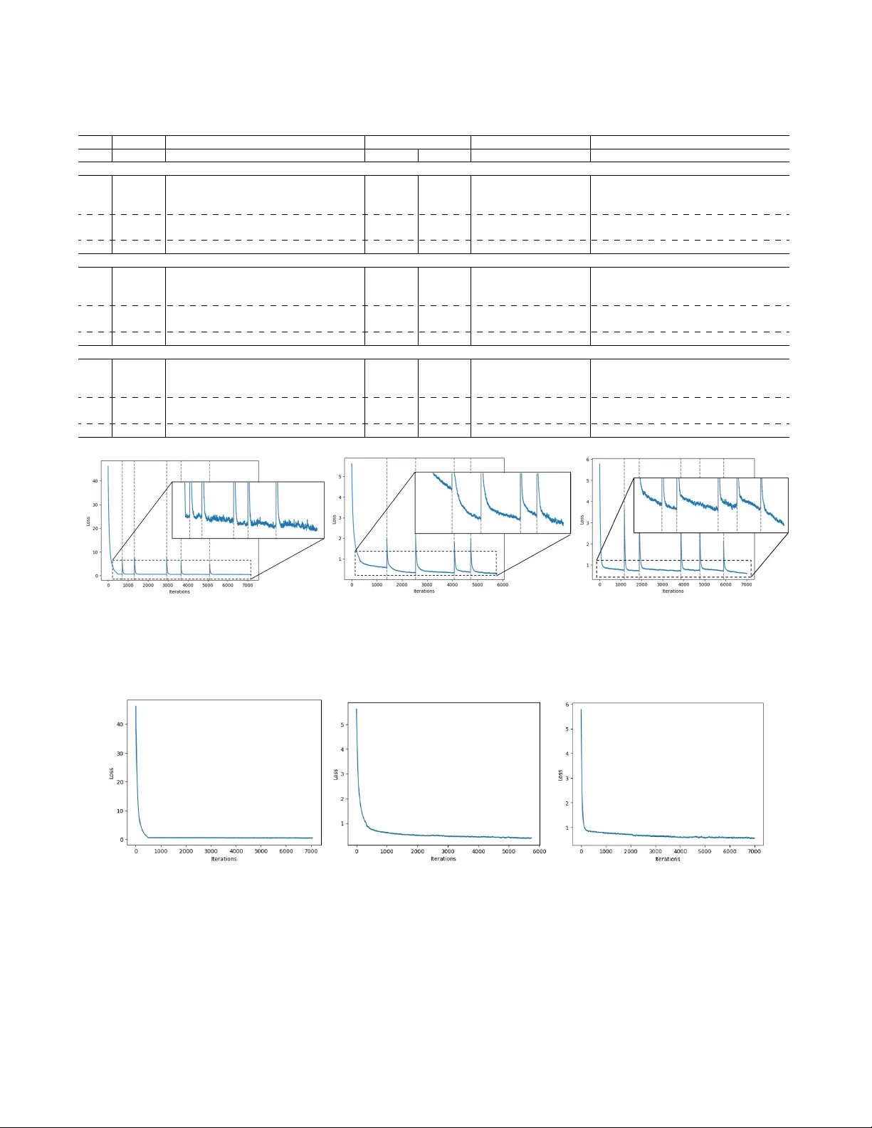
DOI: HTTP://DOI.ORG/10.1109/T AI.2025.3552057 1 GradCF A: A Hybrid Gradient-Based Counterfactual and Feature Attrib ution Explanation Algorithm for Local Interpretation of Neural Networks Jacob Sanderson, Hua Mao, and W ai Lok W oo Senior Member , IEEE, Abstract —Explainable Artificial Intelligence (XAI) is increas- ingly essential as AI systems are deploy ed in critical fields such as healthcare and finance, offering transpar ency into AI-driven decisions. T wo major XAI paradigms, counterfactual explana- tions (CFX) and featur e attribution (F A), serve distinct roles in model interpr etability . This study introduces GradCF A, a hybrid framework combining CFX and F A to improv e inter pretability by explicitly optimizing feasibility , plausibility , and diversity—k ey qualities often unbalanced in existing methods. Unlike most CFX resear ch focused on binary classification, GradCF A extends to multi-class scenarios, supporting a wider range of applications. W e evaluate GradCF A ’ s validity , proximity , sparsity, plausibility , and diversity against state-of-the-art methods, including W achter , DiCE, CARE f or CFX, and SHAP for F A. Results show GradCF A effectively generates feasible, plausible, and diverse counterfactu- als while offering valuable F A insights. By identifying influential features and validating their impact, GradCF A advances AI interpr etability . The code for implementation of this work can be f ound at: https://github .com/jacob- ws/GradCFs Impact Statement —GradCF A offers a r obust, locally explain- able framework f or neural networks by combining counterfactual and feature attrib ution (F A) methods, optimized for feasibil- ity , plausibility , and diversity . This hybrid approach enhances applicability across sectors such as economics, healthcare, law , and en vironmental management. By integrating F A, GradCF A pro vides deeper insights into model beha vior , identifying the influence of each feature in counterfactual generation. Represent- ing a technological leap in AI interpretability , GradCF A helps meet legal standards f or transparency and addresses the social demand for ethical, accountable AI in high-stakes settings. Its extension to multi-class problems further supports broad, r eal- world applicability . Index T erms —Counterfactual Explanations, Featur e Attribu- tion, Explainable AI, Inter pretable Machine Learning I . I N T R O D U C T I O N A S artificial intelligence (AI) increasingly permeates fields like healthcare [ 1 ], cancer detection [ 2 ], credit scoring © 2025 IEEE. Personal use of this material is permitted. Permission from IEEE must be obtained for all other uses, in an y current or future media, including reprinting/republishing this material for advertising or promotional purposes, creating ne w collectiv e works, for resale or redistribution to serv ers or lists, or reuse of any copyrighted component of this work in other works. This is the accepted version of the paper published in IEEE T ransactions on Artificial Intelligence. The final version is av ailable at DOI: http://doi.org/ 10.1109/T AI.2025.3552057 . This work was partly funded through the UK government’ s Flood and Coastal Resilience Innov ation Programme (FCRIP). FCRIP is funded by DEFRA and managed by the Environment Agency . J. Sanderson, H. Mao, and W .L. W oo are with Department of Computer and Information Sciences, Northumbria Uni versity , Ne wcastle, UK, NE1 8ST (e-mail: jacob .sanderson@northumbria.ac.uk; hua.mao@northumbria.ac.uk; wailok.woo@northumbria.ac.uk). [ 3 ], loan prediction [ 4 ], legal decision-making [ 5 ], and disaster relief [ 6 ], the need for transparency has become paramount. Explainable AI (XAI) therefore aims to make AI models more interpretable and trusted in these critical applications [ 7 ]. Feature attribution (F A) is a widely used XAI approach that scores the importance of input features, clarifying model de- cisions and supporting real-world deplo yment. Counterfactual explanations (CFX), another XAI technique, explain decisions by identifying input changes that could alter outcomes. This enables users to see cause-ef fect relations in AI predictions, a high level of interpretability in Pearl’ s hierarchy [ 8 ], providing actionable information for recourse [ 9 ]. CFX fosters user trust by illustrating ho w input changes can impact outputs, re vealing the model’ s internal logic in an intuitiv e way . This capability is increasingly seen as critical in building trustworthy AI systems [ 10 ]. For practical use, CFX must generate feasible and realistic counterfactuals. The CFX community identifies sev eral attributes of ef fecti ve counterfactuals: validity (whether the counterfactual instance is correctly classified), proximity (closeness to the original instance), sparsity (number of changed features), plausibility (alignment with data distribution), and diversity (range among counterfactuals) [ 11 ]. Most CFX methods [ 9 ], [ 11 ], [ 12 ] optimize only a subset of these qualities, often relying on user constraints for feasibility and plausibility , and genetic algorithms for diversity . How- ev er , user reliance can limit diversity , while gradient-descent, another optimization method, often restricts exploration and can reach only local optima. Although genetic algorithms can enhance e xploration, they may produce less precise results and yield overly numerous solutions, which complicates in- terpretability . Despite complementary strengths, F A and CFX have lim- itations when applied individually . While CFX supports ac- tionable insights, it may be limited in interpreting model behavior , especially when counterfactual sets are lar ge. Here, F A can provide more general interpretability , ho wev er , these approaches are limited in their actionable specificity . Existing F A methods like SHAP can be used alongside CFX, but they operate independently , which complicates the implementation by requiring separate integration of multiple post-hoc explain- ers. CFX research is further limited, as existing studies are restricted to binary classification [ 9 ], [ 11 ]–[ 13 ], making multi- class CFX underexplored, though essential, as man y real-w orld applications in volve complex multi-class decision boundaries. 2 DOI: HTTP://DOI.ORG/10.1109/T AI.2025.3552057 In addition, a critical, yet frequently overlook ed aspect of CFX research is the explainability of the counterfactual generation process itself. In this study , we introduce GradCF A, a hybrid CFX and F A algorithm, that generates counterfactuals optimized for prox- imity , sparsity , plausibility , and di versity , while providing F A scores to explain model behavior . This inte gration eliminates the complexity of implementing CFX and F A independently , providing a streamlined solution that supports practical deploy- ment. Furthermore, the F A scores are computed dynamically during counterfactual generation, of fering insights into the feature-specific contributions at e very step of the optimization process. This ensures transparency in how counterfactuals are derived, enhancing user trust in both the outcomes and the methodology . GradCF A further extends the applicability of CFX to multi-class problems, overcoming the common restriction to binary classification and enabling robust e xpla- nations for more complex decision boundaries. These insights are essential in high-stakes contexts, where understanding both counterfactual recommendations and underlying model reasoning supports trust and practical application. GradCF A contributes to the XAI literature by: (i) Optimizing validity , proximity , sparsity , plausibility , and div ersity , incorporating perturbations to escape local op- tima and allowing user control ov er the optimization process. (ii) Providing F A scores by computing gradients with re- spect to input features, allowing both interpretability and actionable insights, while shedding light on the counterfactual generation process. (iii) Extending CFX to multi-class problems, enhancing trust- worthiness and interpretability across a wider range of real-world applications. This paper is organized as follows: Section 2 revie ws exist- ing work in CFX and F A. Section 3 outlines our methodology , Section 4 presents experimental results, Section 5 presents the discussion, and Section 6 concludes with future directions. I I . R E L A T E D W O R K The concept of CFX was first introduced by W achter et al. [ 14 ], defining a CFX as the closest instance with a dif- ferent classification from the original. Their method generates counterfactuals close to the original instance but lacks some qualities desirable for rob ust CFX. DiCE [ 15 ], a widely used extension, addresses this by enhancing diversity through a loss function term that maximizes pairwise distances between instances, giving users multiple interv ention options. While DiCE introduces user constraints for feasibility , it does not account for sparsity or plausibility . Subsequent approaches build on these limitations, for in- stance DECE [ 16 ] enhances sparsity by restricting changes to the top k influential features, impro ving feasibility b ut not plausibility . In [ 17 ] plausibility is considered by optimizing the local outlier factor to ensure counterfactual realism, though this method lacks the di v ersity and feasibility of prior work. Genetic algorithms have also been explored for CFX, as in [ 18 ], adapting W achter’ s approach to optimize for div erse solutions across a larger search space. While effecti ve in escaping local optima and generating diversity , genetic algo- rithms tend to be less efficient than gradient-descent-based methods. In [ 19 ], counterfactuals are used to analyze model robustness to perturbation, focusing on proximity and classi- fication constraints. Other multi-objectiv e CFX methods in- clude NSGA-II [ 20 ] and CARE [ 21 ], which optimize validity , soundness, and actionability alongside proximity and sparsity . CARE emphasizes coherency between changed and unchanged features, providing user-aligned counterfactuals with a focus on minimizing feature adjustments. Most existing CFX methods assume a binary classifier, with limited exploration of CFX for multi-class problems. Multi-class counterfactuals in [ 22 ] rely on support v ector data descriptions (SVDD), which hav e limitations with complex, high-dimensional data. Similarly , in [ 23 ] fuzzy decision trees are applied for rule-based multi-class explanations, offering interpretability but limited handling of complex data. Despite advances, there remains a need for methods that directly optimize div ersity , plausibility , and feasibility , especially in multi-class contexts. In F A, popular methods span model-agnostic and model- specific techniques. LIME [ 24 ] uses a surrogate model for local approximations, while Anchors [ 25 ] identifies feature conditions for high-confidence predictions. SHAP [ 26 ] ap- plies game-theoretic Shapley values for consistent attribu- tion, though it is computationally intensive. Model-specific approaches include Layerwise Relev ance Propagation (LRP) [ 27 ], which traces relevance scores, and Grad-CAM [ 28 ], which uses heatmaps to sho w image regions relev ant to CNN predictions. Each of these methods has unique strengths and trade-offs, such as LRP’ s layer-wise detail and Grad-CAM’ s intuitiv e visualization. I I I . M E T H O D O L O G Y A. V alidity The validity of a counterfactual refers to whether it is correctly classified as the desired class y ′ . In binary classi- fication, this means the class changes, while in multi-class classification, it changes to a specified value. This can be ensured by using a standard loss function, minimizing the distance between the predicted probability and the target class. GradCF A of fers a choice between two loss functions for binary classification problems, hinge loss, and binary cross entropy (BCE) loss. Hinge loss aims to maximise the margin between the two classes, ensuring a clearer boundary between the query instance and counterfactual instances, as follows: L hing e v al = max (0 , 1 − y · f ( x ′ )) (1) where y ∈ {− 1 , +1 } is the target outcome, with − 1 indicating a negati ve class, and +1 indicating positiv e, and f ( x ′ ) is the predicted outcome of a counterfactual instance. BCE loss, on the other hand, quantifies the dif ference between the probability output by the model with the original class, as follows: J. SANDERSON et al. : GRADCF A: HYBRID GRADIENT -BASED COUNTERF A CTU AL AND FEA TURE A TTRIBUTION EXPLANA TIONS 3 L B C E v al = − 1 n n X i =1 [ y ′ i log ( p i ) + (1 − y ′ i ) log (1 − p i )] (2) where n is the number of instances in the counterfactual set, y ∈ { 0 , 1 } is the tar get class, with 0 representing the negati ve class, and 1 the positiv e class, p is the probability of an instance belonging to the positiv e class, and by extension 1 − p is the probability of an instance belonging to the negati ve class. This option is better suited where the goal is to generate counterfactuals that closely resemble the desired class, probabilistically . B. F easibility The feasibility of a counterfactual refers to how easily a suggested modification could be implemented by a user . T o encourage feasible results, we include two terms in the loss function: proximity and sparsity . Proximity ensures that the changes to feature v alues are small, while sparsity ensures that few features are changed. 1) Proximity: T o determine the proximity of the CFX we follow W achter et al. [ 14 ], and measure the average feature- wise absolute dif ference between the original instance x and the counterf actual instance x ′ . T o ensure the features are within the same scale, each feature is normalized by dividing by its median absolute deviation (MAD) v alue. The proximity metric is computed as follows: L prox = 1 nm n X i =1 m X j =1 | x ′ i,j − x j | M AD j (3) where m is the number of features in each instance. 2) Sparsity: T o measure the sparsity of the counterfactuals, we use a boolean operator to determine whether the feature has changed from x to x ′ , meaning the change is greater than ϵ , as defined by the user . W e then sum the dif ferences, giving the total number of features changed, then take the average of this value across the counterfactual set, as follows: L spars = 1 nm n X i =1 m X j =1 1 ( | x ′ ij − x j | ≥ ϵ ) (4) C. Plausibility W e base our plausibility measurement on the fourth objec- tiv e proposed by Dandl et al. [ 20 ], which measures the distance between x ′ with the nearest k instances in the observed data X as an approximation of how likely x ′ is to be in X . W e scale this value by the minimum and maximum distances to normalize the loss value between 0 and 1, as follo ws: L plaus = 1 n n X i =1   1 k k X j =1 | x ′ i − x j | − d min d max − d min + ϵ   (5) where d min and d max are the minimum and maximum dis- tances among the k nearest instances, respecti vely . 1) User Constr aints: The plausibility metric gi ven in equa- tion 5 pro vides an approximation of ho w realistic x ′ may be. In real-world applications, howe ver , there may be specific feature changes that are not possible. In order to ensure real-world plausibility , we incorporate a range of constraints that enable the user to restrict these changes as necessary . F ollo wing DiCE [ 15 ], we enable users to specify features to vary , as well as acceptable ranges for feature v alues. By def ault, all features are permitted to vary , otherwise users can provide a list of features. This is then used to mask the counterfactual instances, such that if a feature is not included in the list its value is replaced with the value from the query instance. For acceptable feature ranges, the default is to bound the features by the minimum and maximum v alues from the observed dataset, but users can specify a dictionary with the feature name as key , and the acceptable range as the v alue. It is beneficial to constrain the features to vary , if the number of features that can be varied is small, but if there are only a fe w features that must remain fixed then this can be a cumbersome option. As such we propose an additional constraint of features to fix, where users specify a list of features to remain fixed, rather than v aried. Finally , there are occasions where a feature may be able to change, but only in one direction. For example, it is plausible for the age of an indi vidual to increase, howe ver it cannot decrease. As such we incorporate an additional constraint on the direction of the feature change, where users specify a dictionary with the feature name as key , and either ‘increase’ or ‘decrease’ as the value. D. Diversity A div erse counterfactual set ensures that a broad range of options are presented to the user, increasing the likelihood of a suitable result being gi ven. This also provides greater insight to approximate the decision boundary of the model. T o measure the di versity of the counterfactual set, we follow the div ersity metric proposed in [ 15 ], measuring the pairwise distance between each pair of instances in the set. W e construct a matrix of these pairwise distances, then find the determinantal point process (DPP) of this matrix, as follo ws: L div = dpp 1 1 + P m l =1 | x ′ il − x ′ j l | ! (6) Unlike the other loss terms (e.g., proximity , sparsity), which are minimized to ensure close, sparse, and plausible counterfactuals, L div is designed to be maximized. This is because higher values of L div indicate a larger div ersity within the counterfactual set, reflecting greater pairwise differences among instances. By maximizing L div , we encourage coun- terfactuals that offer distinct alternati ves, rather than closely clustered solutions. E. Optimization T o optimize the counterfactual set, we construct a loss function from the above defined terms, gi ven in Equation 7 . Our loss function is a weighted sum of the terms, where users 4 DOI: HTTP://DOI.ORG/10.1109/T AI.2025.3552057 can provide a weight for the proximity , sparsity , plausibility , and diversity terms, enabling them to customize the results to their preferences. W e aim to maximise the di versity , so we in v ert it by taking 1 − L div , such that as this term is minimized, the div ersity itself is maximised. The total loss function is computed as follows: L = L v al ( f ( x ′ ) , y ′ ) + λ prox · L prox ( X ′ , x )+ λ spars · L spars ( X ′ , x ) + λ plaus · L plaus ( X ′ , X )+ λ div · (1 − L div ( X ′ )) + L cat ( X ′ ) (7) The term L cat is a regularization term for cate gorical features, to ensure that when one hot encoded, each component of the feature sums to 1. This is enforced through a linear equality constraint, which iterates over each feature and the squared de viation of the sum of the probabilities is computed for each of the cate gories as follows: L cat = X v ∈ cat n X i =1     v last X j = v f ir st x ′ ij   − 1   2 (8) where v ∈ cat denotes the one hot encoded indices of each categorical feature, with v f ir st representing the first index, and v last representing the last index for each cate gorical feature. For each of the terms for the characteristics L char = L prox , L spars , L plaus , if the loss value does not meet a user defined threshold τ char = τ prox , τ spars , τ plaus we add an additional penalty , scaled by user-defined scale factor γ , to more aggressiv ely optimize that term as follo ws: L char = ( L char , if L char ≤ τ char . L char (1 + γ char ) , otherwise . (9) Since we are maximising div ersity L div , for this term we apply the penalty if the loss value exceeds the user defined threshold τ div , with the penalty being a subtraction rather than addition, computed as follows: L div = ( L div , if L div ≥ τ div . L div (1 − γ char ) , otherwise . (10) W e minimize our loss function using the Adam optimizer [ 29 ], which adapts learning rates based on the first and second moments of the gradients, ensuring efficient and robust con- ver gence. A key challenge with gradient-based optimizers is their tendency to get stuck in local optima. T o address this, we implement an optimization strategy where, after con vergence, we check if the overall loss meets a user-defined threshold τ loss . If the loss exceeds this threshold, indicating suboptimal results, we perturb the feature values to escape the local optima and re-run the optimization. This process repeats until the loss is acceptable or a maximum number of perturbation attempts is reached. The perturbation is achiev ed by introducing random noise, sampled from a normal distribution, to each feature that differs from the original instance by more than ϵ . W e select these features for perturbation such that we do not compromise the sparsity of the returned counterfactual set. This random noise is multiplied by a scale factor γ pert , defined by the user, and added to the counterfactual feature v alue as follows: x ′ i = x ′ i + γ pert · N (0 , 1) (11) where N (0 , 1) represents the random noise sampled from a normal distribution. F . Handling Multi-Class Pr oblems While the majority of work in CFX assumes a binary classifier , we argue that this is not sufficient for practical application, as man y crucial real-world problems feature mul- tiple classes, such as income brackets, credit scores, cancer stages and obesity lev els. Multi-class classification is a more complex decision-making problem, due to its multiple, often ov erlapping decision boundaries. Ensuring that GradCF A can handle these problems broadens its real-world utility , of fering a flexible option to stakeholders. The most crucial element to consider when extending from binary to multi-class classification is the v alidity loss term. This term is fundamental in guiding the correct classification of the generated counterfactual instances. In multi-class prob- lems this differs from binary , as there are multiple class prob- abilities to consider . For the validity loss term we implement cross entropy loss, as it inherently handles multiple classes by summing the ne gati ve log probabilities of the correct class, ensuring that the loss calculation accurately reflects the discrepancy between the predicted and desired classes. Cross entropy loss in multi-class problems is computed as follows: L v al = − 1 n n X i =1 cl X j =1 y ′ ij log ( p ij ) (12) where cl is the number of classes. G. F eatur e Attribution T o enhance the interpretability of the system, GradCF A also provides F A scores, gi ving the importance of each feature in the counterfactual generation process. This is achiev ed by calculating the gradients ∇ x ′ f ( x ′ ) which denote the partial deriv atives of the predicti ve model’ s output f ( x ′ ) with respect to the input features x ′ i ∈ x ′ . These gradients are computed through backpropagation, and are accumulated across each optimization step to give the cumulativ e impact of each feature x ′ i on the counterfactual prediction. The accumulated gradients are then averaged over the optimization steps, and their magnitude (norm) is used to quantify each feature’ s importance. The attribution score for each feature Attr i can therefore be giv en as follows: ∇ ti = ∂ f ( x ′ i,t ) ∂ x ′ i,t (13) Attr i =      1 T T X t =1 ∇ ti      (14) where T is the total time steps, x ′ t is the counterfactual instance at time step t . An overvie w of the GradCF A workflow is giv en in Algorithm 1 and Fig. 1 . J. SANDERSON et al. : GRADCF A: HYBRID GRADIENT -BASED COUNTERF A CTU AL AND FEA TURE A TTRIBUTION EXPLANA TIONS 5 Fig. 1: Overview of the GradCF A Pipeline: Beginning with a trained neural network, a query instance, and the observed dataset. The counterfactual set X ′ is initialized with random v alues sampled from a normal distrib ution. Indi vidual loss components are calculated and compared with user-defined thresholds τ char , where each loss component L has its own threshold τ char . For proximity , sparsity , and plausibility L within τ is true if L ≤ τ char , and for div ersity L is considered within τ if L ≥ τ char . If thresholds are not met, a penalty is applied. The total loss is computed based on user-defined weighting. User constraints are then applied, gradients are computed to attribute feature importance, and update X ′ . If the final loss after optimization does not meet the threshold, values are perturbed, and optimization is repeated until an acceptable loss is achiev ed or the maximum number of perturbation attempts is reached, after which the counterfactual set and F As are returned. H. T ime Complexity The GradCF A framework combines CFX and F A, optimiz- ing multiple qualities that contribute to increased computa- tional ov erhead compared to simpler methods. T o ev aluate scalability , we analyze the time complexity . The loss function consists of six components—validity , proximity , sparsity , plausibility , diversity , and categorical regu- larization—each with distinct computational demands. V alidity is computed once per counterfactual, with complexity O ( n ) where n is the number of counterfactuals. Proximity and sparsity are computed over features, and their complexity is O ( n · m ) . When the feature count m is constant, this simplifies to O ( n ) , howe ver if m grows significantly the complexity scales linearly with m . Plausibility requires finding k -nearest neighbors, contributing O ( n ) as k is fixed. The div ersity calculation, which inv olves a matrix determinant, has complexity O ( n 3 ) , making it the dominant term as n increases. During optimization, GradCF A iterati vely updates X ′ to minimize the loss, requiring gradient computation with respect to X ′ . Each gradient step has complexity O ( n ) with a fixed feature count m . Gi ven a maximum iteration count µ , the complexity for optimization becomes O ( µ · n ) . The total time complexity of GradCF A is therefore: O ( n 3 + µ · n ) (15) The dominant term O ( n 3 ) stems from the di versity com- ponent, meaning that scaling primarily depends on n . How- ev er , m could factor into the time complexity if it gro ws significantly , affecting both O ( n ) terms in loss calculation and optimization. F or most applications, constants lik e maximum perturbations δ remain negligible, but the ov erall runtime could increase with high feature counts. Moreov er , n should remain relati vely low to ensure inter- pretability , as a large set of counterfactuals could overwhelm users with redundant information. By managing n and setting a reasonable iteration limit µ , GradCF A achieves a balance be- tween computational feasibility and high-quality , interpretable counterfactual explanations. I. Evaluation W e e v aluate GradCF A on the proximity , sparsity , di versity , and plausibility loss values for the final set of counterfactuals returned. W e e valuate the validity of the counterfactuals by measuring the confidence of the classification of the counter- factuals, which we define as the probability assigned by the predictiv e model to the desired class. For proximity , sparsity , and plausibility , a low value is desirable, while for diversity and validity and high v alue is preferred. Since the goal is not to excel in any one criteria, but to obtain the best ov erall balance, we look for the best average of the fiv e main criteria. Since Proximity , Sparsity , and Plausibility are minimized, we use 1 − each of these v alues in calculating the average, so a higher av erage score indicates superior performance. 6 DOI: HTTP://DOI.ORG/10.1109/T AI.2025.3552057 Algorithm 1 GradCF A Input : Query Instance x , Predictiv e Model f ( · ) , Hyperparameters θ Parameter : Learning rate α , W eights λ , Thresholds τ , Scale Factors γ , Maximum Iterations µ , Maximum Perturbation Attempts δ , Number of Counterfactual Instances in the Set n Output : Counterfactual Set X ′ , Feature Attributions Attr 1: Let iteration count t = 0 , perturbation count p = 0 , X ′ ← N (0 , 1) n × len ( x ) , Attr ← 0 2: while t < δ or D l ≥ τ ld do 3: Compute loss components L v al , L di , L pl , L pr , L sp , L cat . 4: for L char in L di , L pl , L pr , L sp do 5: if L char > τ char then 6: L char ← L i (1 − γ char ) 7: end if 8: end for 9: Compute total loss L ← L v al + λ prox · L prox + λ spars · L spars + λ plaus · L plaus + λ div · L div + L cat . 10: Compute gradients ∇ of L w .r .t X ′ . 11: Compute gradients ∇ of f ( x ′ ) w .r .t x ′ i 12: Append gradient ∇ x ′ f ( x ′ ) to gradients list Attr 13: Update X ′ with gradient descent with learning rate α . 14: Apply user constraints. 15: D l ← L t − L t − 1 16: if t ≥ δ or D l < τ ld then 17: break 18: end if 19: t = t + 1 20: end while 21: if L > τ pert then 22: while p < δ do 23: X ′ ← X ′ + N (0 , 1) · γ pert 24: t = 0 25: Go to step 2. 26: if L ≤ τ pert then 27: retur n X ′ 28: end if 29: p = p + 1 30: end while 31: end if 32: for feature x i , gradient ∇ i in Attr do 33: Attr ←    1 T P T t =1 ∇ ti    34: end f or 35: return X ′ with lowest L { Return the set of counterfactual instances with the lowest total loss. } 36: return Attr { Return the attribution v alues for each fea- ture. } 1) Datasets: T o e v aluate our framework we use three datasets, one for binary classification, and two for multi- class, with one having a larger number of features. F or binary classification we use the credit approval dataset from the UCI Machine Learning Repository [ 30 ], which contains 690 instances of 14 features, with 4 continuous, and 10 categorical. For multi-class classification we use the obesity lev els dataset, also from the UCI Machine Learning Repository [ 31 ], which contains 2111 instances of 16 features, 6 of which are continuous, 10 are categorical. This dataset has 7 classes ranging from underweight, to le vel 3 obesity . W e also use a larger dataset from the UCI Machine Learning Repository for the classification of fetal health through cardiotocography data [ 32 ]. This dataset has 2126 instances of 32 features, of which 22 are continuous, and 10 are categorical. This dataset has 3 classes, normal, suspect and pathological. Prior to model training, the continuous features are scaled by the mean and standard deviation, and the categorical features are one hot encoded. T o train the predicti ve model we split each dataset into train- ing, validation, and testing sets, with a ratio of 60:20:20. Grad- CF A is ev aluated post-hoc on the test set of the pre-trained predictiv e model. Its performance is assessed by av eraging the results of each metric across all test instances, providing a fair representation of its capabilities. The continuous features are scaled using z-score normalization, and categorical features are one hot encoded. T o address any missing values in the datasets we drop the corresponding ro w , as imputation with artificial values may impact the integrity of the counterfactual explanations. J. Experimental Setup 1) Predictive Model: While GradCF A is not a trainable model, it le verages the classification ability of a pretrained predictiv e model. In our experiments, we use a fully connected neural network with an input layer, followed by 2 hidden layers, the first with 64 neurons, the second with 32, and an output layer . F or binary classification a sigmoid acti v ation function is used, while for multi-class we use softmax. W e leav e the exploration of GradCF A as an explainer for other types of neural network for future w ork. While the optimiza- tion of the predicti ve model is beyond the scope of this study , it is essential to ensure that the models achiev e reasonable accuracy , as this directly impacts the validity and plausibility of the counterfactual results. T able I presents the classification accuracy of the predictive model on the training, validation, and testing sets for all three datasets used in this study . These results indicate that the models are suf ficiently accurate to support meaningful counterfactual explanations. T ABLE I: Classification accuracy of the predicti ve model on each dataset across training, v alidation and testing. Dataset T raining V alidation T esting Credit Approval 0.88 0.86 0.82 Obesity 0.90 0.84 0.85 Fetal Health 0.92 0.93 0.91 2) Hyperparameter T uning: GradCF A has several hyperpa- rameters to tune, we select the values for each hyperparameter through a grid search of different values over the test set, with the following ranges: • λ : [0.25, 0.5, 0.75, 1.0] • γ pen : [0.05, 0.1, 0.15, 0.2] • γ pert : [0.3, 0.5, 0.7, 0.9] J. SANDERSON et al. : GRADCF A: HYBRID GRADIENT -BASED COUNTERF A CTU AL AND FEA TURE A TTRIBUTION EXPLANA TIONS 7 • τ prox , τ spars , τ plaus : [0.1, 0.2, 0.3, 0.4, 0.5] • τ d iv : [0.5, 0.6, 0.7, 0.9] • τ loss : [0.3, 0.4, 0.5, 0.6, 0.7] For λ we choose a v alue of 0.5 for each term, giving the best balance of the proximity , sparsity , plausibility and div ersity metrics with the validity of the counterfactuals, while ensuring uniformity for comparison, in particular with previous w ork. W e find a γ pen value of 0.1 to provide the best scaling for the additional penalty , striking a balance between being suitably aggressiv e to optimize the characteristics, while maintaining throughout the process. For the credit approv al dataset we find τ prox and τ spars values of 0.2, τ plaus of 0.4, and τ div of 0.9 to be the most optimal. For the obesity lev els problem we find the optimal v alues to be 0.3 for τ prox and τ spars , and 0.4 for τ plaus and τ div . For the fetal health dataset we find τ prox and τ spars of 0.4, τ plaus of 0.5 to provide optimal results. For all datasets, we find a γ pert value of 0.5 to pro vide a suitably lar ge perturbation to escape local optima, while still maintaining the knowledge gained through the previous optimization step. For credit approv al, a τ loss of 0.5 is selected for optimal results, while for obesity a value of 0.4, and for fetal health a slightly higher value of 0.6 is necessary . 3) Baseline Models: In our experiments we compare our work with three benchmark CFX algorithms, including W achter [ 14 ], DiCE [ 15 ] and CARE [ 21 ]. W achter serves as our baseline due to its seminal status in counterfactual gener- ation, upon which many subsequent algorithms are founded. DiCE is chosen as it remains the state-of-the-art and is widely recognized as the leading algorithm for CFX generation tasks. Lastly , CARE is selected as it represents a recent advancement in CFX, and also pro vides a vie w of ho w the use of a genetic multi-objectiv e algorithm performs in comparison with gradi- ent descent-based approaches. Each algorithm is implemented using Python libraries published by the authors. I V . R E S U LT S A. Ablation Study T o demonstrate the improv ed quality achieved through the inclusion of sparsity , plausibility and div ersity , we perform an ablation study . Giv en the definition of a CFX as the smallest changes to the input features required to change the classification of the model, validity and proximity are integral components of a CFX algorithm, so we include these two components in each combination. Therefore, the follo wing combinations are considered: 1) V alidity and Proximity only , 2) V alidity , Proximity , and Sparsity , 3) V alidity , Proximity , and Plausibility , 4) V alidity , Proximity , and Div ersity , 5) V alidity , Proximity , Sparsity , and Plausibility , 6) V alidity , Proximity , Sparsity , and Div ersity , 7) V alidity , Proximity , Plausibility , and Div ersity , and 8) V alidity , Proximity , Sparsity , Plausibility , and Div ersity (GradCF A). The results of this ablation study are provided in T able II , under the heading ‘ Ablation Study Combinations’, with combination 8 under the ‘GradCF A ’ heading. This T able sho ws that for credit approv al, combinations 1, 2, and 6 produce the closest and most sparse counterfactuals. Howe ver , these combinations suf fer in plausibility , div ersity , and validity . Combinations 3, 4, and 5 of fer moderate proximity and spar- sity , with slight improvements in plausibility for combinations 3 and 5, though still weak overall. Combination 7 excels in plausibility and div ersity but trades off proximity and sparsity , showing the weakest performance in these areas. Combination 8, the proposed loss function in GradCF A, strikes a balance, achieving moderate proximity and sparsity while e xcelling in plausibility , div ersity , and validity . For obesity le vels, combination 1 again offers the lowest proximity , with combinations 2 and 6 also performing well in this reg ard but poorly in div ersity . Combinations 3, 4, and 5 achieve moderate proximity , b ut 3 and 5 sho w lo w div ersity , particularly compared to their performance on the credit approv al data. These combinations also hav e better plausibility but higher sparsity scores. Combination 8, the GradCF A function, balances all metrics, with the best plau- sibility , strong sparsity and di versity , and moderate proximity . In the fetal health dataset, we observe that again, combi- nation 1, 2, and 6 maintain the lowest proximity and sparsity scores, with relativ ely weak div ersity and plausibility . Com- binations 3, 4, 5, and 7 all achiev e comparable performance across proximity , plausibility , and diversity , ho we ver combi- nation 5 achieves a much better sparsity score. As in the other two datasets, GradCF A achiev es the best balance across all metrics, with the highest validity and div ersity scores, lowest plausibility score, and moderate proximity and sparsity . B. P erturbation Analysis T o assess the effecti veness of perturbation in escaping local optima and improving counterfactual quality , Fig. 2 sho ws the loss curve throughout optimization for each dataset. Fig. 3 shows the loss curv e for the same number of iterations, without perturbation. Additionally , T able II sho ws the results with the perturbation strategy , as ‘GradCF A ’ as well as the results without the perturbation strate gy as ‘W/o Pert’. The loss curves show that perturbation enables the algorithm to achiev e a lo wer o verall loss, resulting in higher-quality counterf actuals. This confirms the strategy’ s ef fecti veness in escaping local optima and achieving more globally optimal results. Across all datasets, the loss value for ev ery metric is improved where perturbation is included in the optimization strategy , further demonstrating the efficac y of this approach. C. Additional P enalty In T able II the performance of GradCF A where the addi- tional penalty is included in the terms L prox , L spars , L plaus and L div is presented under ‘W/o Pen’. Across all datasets, it can be observed that the inclusion of the additional penalty , shown under ‘GradCF A ’ is effecti ve in driving a better perfor- mance against each metric. Additionally , all of the results fall within the threshold value provided, demonstrating how effec- tiv ely the performance can be controlled through GradCF A. D. Example Counterfactuals In T ables III , IV , and V , example counterfactual sets are provided for the credit approval, obesity lev els, and fetal 8 DOI: HTTP://DOI.ORG/10.1109/T AI.2025.3552057 T ABLE II: Proximity , Sparsity , Plausibility , Div ersity and Confidence of GradCF A in Comparison with the results obtained in the e xperiments conducted in subsections IV A, B, C, E, and F . Proximity , Sparsity and Plausibilty are minimized, while Div ersity and V alidity are maximized. An o verall a verage of these metrics is given for each experiment. Ablation Study Combinations GradCF A Previous W ork Multi-Class GradCF A 1 2 3 4 5 6 7 W/o Pert. W/o Pen. W achter DiCE CARE 0 1 2 3 4 5 6 Credit Approval Dataset for Binary Classification Prox. 0.15 0.14 0.12 0.19 0.16 0.16 0.13 0.23 0.23 0.21 0.03 0.12 0.18 - - - - - - - Spars 0.18 0.19 0.16 0.21 0.20 0.20 0.17 0.25 0.27 0.24 0.10 0.28 0.56 - - - - - - - Plaus 0.37 0.68 0.53 0.61 0.46 0.45 0.54 0.42 0.51 0.45 0.56 0.51 0.47 - - - - - - - Div 0.96 0.86 0.72 0.82 0.92 0.80 0.88 0.94 0.91 0.92 0.35 0.84 0.68 - - - - - - - Conf. 0.78 0.76 0.74 0.76 0.71 0.78 0.73 0.72 0.75 0.70 0.56 0.64 0.66 - - - - - - - A vg. 0.81 0.76 0.73 0.71 0.76 0.75 0.75 0.75 0.73 0.74 0.64 0.71 0.63 - - - - - - - Obesity Levels Dataset for Multi-Class Classification Prox. 0.21 0.06 0.24 0.26 0.17 0.24 0.16 0.26 0.35 0.37 - - - 0.21 - 0.21 0.22 0.26 0.29 0.35 Spars 0.23 0.25 0.25 0.32 0.29 0.25 0.36 0.20 0.35 0.40 - - - 0.25 - 0.23 0.27 0.23 0.26 0.31 Plaus 0.34 0.50 0.70 0.52 0.50 0.53 0.48 0.47 0.45 0.51 - - - 0.39 - 0.34 0.52 0.59 0.61 0.67 Div 0.92 0.04 0.11 0.79 0.84 0.64 0.42 0.82 0.80 0.83 - - - 0.90 - 0.92 0.87 0.84 0.85 0.83 Conf. 0.76 0.68 0.79 0.74 0.71 0.78 0.68 0.76 0.73 0.69 - - - 0.71 - 0.76 0.73 0.70 0.67 0.64 A vg. 0.78 0.58 0.54 0.69 0.72 0.68 0.62 0.73 0.68 0.65 - - - 0.75 - 0.78 0.72 0.69 0.67 0.63 Fetal Health Dataset for Multi-Class Classification Prox. 0.34 0.29 0.33 0.47 0.46 0.35 0.29 0.46 0.40 0.45 - - - - 0.34 0.36 - - - - Spars 0.35 0.51 0.31 0.52 0.51 0.40 0.33 0.52 0.51 0.49 - - - - 0.35 0.39 - - - - Plaus 0.42 0.56 0.51 0.42 0.49 0.48 0.63 0.45 0.54 0.47 - - - - 0.42 0.52 - - - - Div 0.96 0.82 0.86 0.89 0.90 0.91 0.83 0.95 0.94 0.93 - - - - 0.96 0.93 - - - - Conf. 0.79 0.78 0.79 0.74 0.72 0.78 0.73 0.74 0.71 0.72 - - - - 0.79 0.76 - - - - A vg. 0.73 0.65 0.70 0.64 0.63 0.69 0.66 0.65 0.64 0.65 - - - - 0.73 0.68 - - - - (a) (b) (c) Fig. 2: Loss curves for (a) credit approv al, (b) obesity le vels, and (c) fetal health, with perturbation, where the grey dashed lines represent the points of perturbation. The curves demonstrate that after each perturbation the loss is dri ven further do wn, indicating the efficac y of the approach in improving the results. (a) (b) (c) Fig. 3: Loss curves for (a) credit approv al, (b) obesity le vels, and (c) fetal health without perturbation. health datasets, respectively . For the credit approval dataset, the initial query instance was classified as 0 (rejection), and counterfactuals were generated for class 1 (approv al). For the obesity dataset, we used a query classified as 2 (overweight lev el 1) and aimed to generate counterfactuals for class 1 (normal weight). Finally , for the fetal health dataset, we used a query initially classed as 1 (suspect) and targeted counterfactuals for class 0 (normal). In the credit appro v al dataset, certain features such as Age and Income stay relativ ely similar to the original instance across counterfactuals. V ariables lik e marital status (MS), bank customer status (BC), and citizenship also remain unchanged, suggesting these may have limited influence on credit ap- prov al. Gender and ethnicity vary minimally as well, implying J. SANDERSON et al. : GRADCF A: HYBRID GRADIENT -BASED COUNTERF A CTU AL AND FEA TURE A TTRIBUTION EXPLANA TIONS 9 that the model is not heavily biased by demographic details in making its decisions. Howe v er , Employment Status (ES) consistently shifts from unemployed to employed in coun- terfactuals, highlighting its significant impact on approval—a pattern that aligns well with real-world expectations. Y ears employed (YE) tends to increase across the counterfactuals, supporting the idea that extended employment is fa vorable for credit approv al. Conv ersely , debt levels and previous defaults (PD) rise in each instance, which is counterintuiti ve as lower debt would generally be preferred. This suggests either an inconsistency in model learning or complex interdependencies among features, where high debt or defaults are acceptable when compensated by other strong indicators. In the obesity le vels dataset, body mass index (BMI) serves as the primary measure, dependent on both height and weight. Here, the generated counterfactuals reflect substantial weight loss for the shift from ov erweight to normal weight. Interest- ingly , there is also a minor reduction in height, which is logi- cally inconsistent with the objectiv e of achieving a lower BMI, howe ver , when coupled with the lower weight this change is still reasonable. Most other features remain consistent, except for the frequency of physical activity (F AF), which decreases in each counterfactual. This unexpected outcome may point to feature dependencies within the model, where reduced physical activity is compensated by significant weight loss. In the fetal health dataset, where the query instance ini- tially indicated a suspect classification, counterf actuals for the normal classification re veal se veral shifts in clinical measure- ments. Features related to long term variability (AL TV , ML TV) generally increase, which suggests that the fetal heart rate is adapting dynamically to conditions, reflecting a healthy auto- nomic nervous system and adequate oxygenation. Con versely , uterine contractions (UC) and deceleration episodes (DL) tend to decrease, aligning with expectations of healthier outcomes. Other features, including accelerations (A C) and mean value (Mean), e xhibit v ariability b ut follow consistent patterns across counterfactuals, indicating their role in distinguishing suspect from normal fetal health. T ABLE III: Example Counterfactual Set for Credit Appro v al. Feature Query Counterfactual V alues Age 34.14 28.55 33.44 35.34 37.26 46.75 Debt 2.75 4.2 3.9 3.4 5.1 8.0 YE 2.5 3.28 3.93 2.94 3.54 2.5 Income 200.01 199.00 200.00 205.00 105.00 195.00 Gender 1 1 1 1 0 0 MS 1 1 1 1 1 1 BC 1 1 1 1 1 1 Industry 1 0 1 1 13 1 Ethnicity 0 4 0 0 0 0 PD 0 1 1 1 1 1 ES 0 1 1 1 1 0 CS 0 2 0 10 0 0 DL 1 1 1 0 1 0 Citizen 0 0 0 0 0 0 Outcome 0 1 1 1 1 1 E. Pre vious W ork T o contextualise the performance of GradCF A, we compare its performance with existing CFX algorithms in T able II T ABLE IV: Example Counterfactual Set for Obesity Lev els. Feature Query Counterfactual V alues Age 19.0 20.0 19.0 21.0 23.0 22.0 Height 1.75 1.68 1.72 1.65 1.66 1.65 W eight 100.0 53.4 51.9 62.3 51.6 61.8 FVFC 2.0 1.9 1.9 1.9 2.0 2.0 NCP 3.0 3.0 3.0 2.9 3.0 3.0 CH2O 2.0 1.9 2.0 2.0 2.0 2.0 F AF 2.0 0.6 1.2 0.8 0.4 0.5 TUE 4.2e-8 4.1e-8 4.2e-8 4.2e-8 4.2e-8 4.2e-8 Gender 1 1 1 1 1 1 CALC 3 2 3 3 3 2 F A VC 1 1 1 1 0 0 SCC 0 0 0 0 0 0 SMOKE 0 0 0 0 0 0 FHWO 1 1 1 1 1 1 CAEC 1 1 1 2 1 2 MTRANS 3 3 3 3 3 3 Outcome 2 1 1 1 1 1 T ABLE V: Example Counterfactual Set for Fetal Health. Feature Query Counterfactual V alues LBE 125.0 128.9 148.0 128.3 141.5 142.2 LB 125.0 132.8 124.9 124.8 132.1 118.2 A C 10.0 5.1 2.8 0.1 5.5 2.2 FM -4.6e-11 -3e-11 -7.4e-11 -1.1e-11 1.5e-11 1.2e-11 UC 2.3e-10 3e-10 -1.2e-10 4.3e-10 -4e-10 -2e-10 ASTV 41.0 56.9 55.1 52.6 44.2 41.0 MSTV 1.2 0.2 0.7 0.8 1.0 1.2 AL TV -2.2e-7 2.1e-7 -1.4e-7 -2.7e-7 2.4e-7 -3.1e-7 ML TV 11.4 21.1 13.2 23.5 27.6 13.6 DL -2.5e-9 -8.9e-9 -1e-9 -4.8e-9 -5.5e-9 -8.1e-9 DS -5.7e-11 -1.9e-11 -2.3e-11 -1.4e-11 -2.9e-11 -2.1e-11 DP 3.2e-10 1.8e-10 1.9e-10 9.7e-11 2.1e-10 1.5e-10 DR 0.0 0.1 -0.1 0.0 0.2 -0.1 W idth 63.0 13.5 16.3 3.2 62.2 30.3 Min 98.0 151.3 117.3 92.4 121.4 128.1 Max 161.0 143.8 134.7 137.9 128.6 129.9 Nmax 4.0 3.7 1.1 2.9 3.8 4.3 Nzeros -4.1e-9 -5e-9 -8.3e-9 -6.1e-9 -7.5e-9 -7.5e-9 Mode 138.0 119.8 113.4 125.5 126.8 131.9 Mean 135.0 134.6 113.1 113.6 88.4 116.4 Median 137.0 120.7 128.9 132.2 140.9 136.9 V ariance 6.0 6.2 2.9 5.1 7.5 3.9 T endency 1 1 0 1 1 0 A 0 0 0 0 0 0 B 1 1 1 1 1 1 C 0 0 0 0 0 0 D 1 1 0 1 1 0 E 0 0 0 0 0 0 AD 0 0 0 0 0 0 DE 0 0 1 0 0 0 LD 0 0 0 0 0 0 FS 0 0 0 0 0 0 SUSP 0 0 0 0 0 0 Outcome 1 0 0 0 0 0 for the credit approv al dataset. As far as the authors are aware, GradCF A is the first CFX algorithm for multi-class problems, therefore we cannot compare with previous work on the obesity levels or fetal health data. In proximity , W achter achiev es the best result, which is expected gi ven that proximity is the main focus of this algorithm. This is followed by DiCE, which focuses on balancing proximity and div ersity . CARE and GradCF A both achiev e a more modest value on this metric, which can be attributed to the increased complexity in their loss functions. W achter also achiev es the best sparsity score, an intuitive extension of close proximity , as the best proximity score is an unchanged feature. GradCF A follo ws 10 DOI: HTTP://DOI.ORG/10.1109/T AI.2025.3552057 this, demonstrating the benefit of explicitly optimizing for this where the loss function is more complex. DiCE does not optimize for sparsity , and achie ves a slightly weaker performance, demonstrating that there is a likely trade-off in sparsity when optimizing for diversity . CARE performs the weakest on this metric, with more than half of the features changing on average. GradCF A significantly outperforms the other algorithms on plausibility , demonstrating that the results generated by this algorithm are closer to the distribution of the observed data, so are more likely to exist as real instances. DiCE and W achter both perform comparably , with DiCE achie ving a marginally lower value. CARE does consider the closeness to the observ ed data in its validity module, which can be attributed to its lower plausibility value. The complexity of CARE, howe ver , does not enable suf ficiently efficient optimization of each compo- nent for it to achieve comparable performance. GradCF A also achiev es the best div ersity score, demonstrating its ability to provide a broad range of counterfactual options to the user . Despite DiCE having a greater focus on di versity , with fe wer competing objectives to optimize for, it follows GradCF A with a diversity score of 0.12 less. CARE follo ws DiCE with a much lo wer div ersity score. CARE does not explicitly optimize for di versity , b ut rather relies on the use of genetic optimization to ensure div ersity , which indicates that genetic optimization is not as effecti ve in generating di verse results as a div ersity loss function term. Finally , W achter achiev es the poorest div ersity score, which is expected, as this algorithm was not intended to provide a diverse set of counterfactuals, b ut rather the closest possible counterfactual instance. Overall the performance of GradCF A is much more balanced across all four characteristics than an y of the pre vious works, demonstrating its efficac y in optimizing for feasibility , plausibility , and di versity . F . Multi-Class Analysis A key contribution of our work is its extension of CFX to multi-class problems, so here we ev aluate the impact of the class of the original instance on the performance against the ev aluation metrics. For obesity , we consider the target class to be 1, which is normal weight, and e valuate counterfactuals generated from query instances of each of the other classes in the dataset. F or fetal health, we consider the target class to be 0, which is a normal fetus. The results of this e valuation are shown in T able II under the heading ‘Multi-Class’. The results show that as the original class gets further from the target class, the proximity of the results gets further in turn. This is an intuitiv e finding, as if we consider the real world scenario of obesity lev els, an indi vidual who is classified as le vel 2 obese will need to lose more weight, and make greater lifestyle changes to become a normal weight, than someone who is lev el 1 ov erweight, for instance. Plausibility also increases as the original class moves further from the target class, indicating that it is easier to generate a more realistic counterfactual from a query instance that is closer to begin with. Sparsity , di versity and v alidity do not sho w any consistent pattern as the class changes. This indicates that these values are not significantly impacted by the original class. G. F eatur e Attribution The F A element of GradCF A informs on the important features for generating feasible, plausible, and div erse coun- terfactuals, giving deeper insight into model interpretation. An example of the F A computed for each dataset is shown in Fig. 4 . In credit approval, prior default and income hav e the highest attribution scores, indicating their crucial role in generating counterfactuals. Conv ersely , age, years employed, and debt hav e much lo wer scores, showing they are less influential. For obesity lev els, weight is the most critical feature, as expected. In contrast, age, ve getable consumption frequency (FCVC), physical activity (F AF), and main meals (NCP) have the lo west attrib ution scores, reflecting their minor role in obesity classification. Lastly , for fetal health, activ e vigilance (D), and calm sleep (A) hav e the highest importance scores, while statistics of the histograms such as median, variance and number of zeros (Nzeros) have significantly lower importance. For comparison, we also compute the feature attrib ution using state-of-the-art method Shapley Additiv e V alues (SHAP) [ 26 ]. In all three cases, the feature deemed most important by SHAP is consistent with the most important feature computed by GradCF A. There is more v ariance in the less important features, howe ver the scale of the attrib ution scores is very small, so these differences are not of particular significance. T o assess the F A, we fix each feature and ev aluate its impact on counterfactual generation in terms of validity , proximity , sparsity , plausibility , and di versity . Results are presented in T able VI for credit approv al, T able VII for obesity le vels, and T able VIII for fetal health. W e e xclude the fixed feature from the metric computation to av oid bias. In credit approval, fixing prior default prev ents counterfactual generation within the maximum iterations, highlighting its critical role. Removing less influential features, impacts counterf actual quality less significantly . For instance, fixing income (the second most influential feature) results in very lo w v alidity (0.54) and weaker metric scores, showing that counterfactuals are less valid and less aligned with desired qualities. This is reflected in a significantly higher plausibility score, indicating the importance of altering income for realistic counterfactuals. Con v ersely , fixing debt (the least influential feature) has min- imal impact, leading to high v alidity and improved metrics, similar to when all features can vary . For the obesity levels data, fixing the most influential feature renders counterf actual generation impossible, with a v alidity score of only 0.18, illustrating the complexity of multi-class classification. Fixing the second-most influential feature, mode of transportation (MTRANS), results in weaker metrics and lower validity in counterfactuals, indicating reduced quality . In contrast, fixing less influential features like NCP and F AF yields metrics similar to when all features vary and maintains higher validity , showing minimal impact on counterfactual generation. For the fetal health dataset the top two features ha ve a much higher attrib ution score than in the other two datasets, and in both cases fixing them prevents successful counterfactual generation. In general it can be observed that as the importance lessens, the counterfactual qualities improve, suggesting that it becomes less challenging to generate actionable counterfactual J. SANDERSON et al. : GRADCF A: HYBRID GRADIENT -BASED COUNTERF A CTU AL AND FEA TURE A TTRIBUTION EXPLANA TIONS 11 (a) (b) (c) Fig. 4: F A computed with GradCF A for (a) credit approv al, (b) obesity lev els and (c) fetal health. The results highlight the critical role of prior def ault and income in credit approval, weight in obesity classification, and active vigilance and calm sleep in fetal health, while other features like age, years employed, dietary habits, and histogram statistics are less influential in generating plausible and feasible counterfactuals. (a) (b) (c) Fig. 5: F A computed with SHAP for (a) credit approv al, (b) obesity levels and (c) fetal health. examples. T ABLE VI: Analysis of the F A with the Credit Approval Data. Feature V al. Prox. Spars. Plaus. Div . Fixed PriorDefault 0.37 - - - - Income 0.54 0.26 0.24 0.87 0.82 Industry 0.62 0.25 0.22 0.61 0.86 CreditScore 0.65 0.24 0.24 0.50 0.88 BankCustomer 0.67 0.23 0.23 0.46 0.88 Driv ersLicense 0.68 0.22 0.24 0.45 0.91 Citizen 0.70 0.22 0.21 0.43 0.90 Married 0.71 0.21 0.22 0.44 0.91 Ethnicity 0.73 0.21 0.21 0.42 0.93 Gender 0.74 0.21 0.23 0.40 0.92 Employed 0.87 0.72 0.20 0.09 0.92 Age 0.76 0.21 0.20 0.39 0.93 Y earsEmployed 0.78 0.22 0.21 0.40 0.95 Debt 0.77 0.20 0.22 0.42 0.94 V . D I S C U S S I O N Across all experiments, GradCF A consistently generates balanced counterfactuals in terms of proximity , sparsity , plau- sibility , and di versity , while maintaining high classification confidence. Our results show that GradCF A ’ s loss function and optimization strategy outperform other configurations across binary and multi-class problems, emphasizing the importance of each element in achieving this balance. This quality balance is crucial for practical utility , ensuring counterfactuals are both feasible and provide a div erse range of realistic options. A major contrib ution of GradCF A is its F A mechanism, which identifies influential features crucial for generating feasible, plausible, and diverse counterfactuals. F A analysis T ABLE VII: Analysis of the F A with the Obesity Lev els Data. Feature V al. Prox. Spars. Plaus. Div . Fixed W eight 0.18 - - - - MTRANS 0.52 0.33 0.42 0.62 0.71 SMOKE 0.57 0.29 0.37 0.67 0.75 CALC 0.59 0.28 0.35 0.61 0.76 CAEC 0.61 0.28 0.30 0.55 0.78 SCC 0.58 0.27 0.31 0.58 0.81 Gender 0.62 0.26 0.30 0.59 0.80 TUE 0.65 0.25 0.33 0.56 0.79 FHWO 0.66 0.25 0.31 0.54 0.82 F A VC 0.67 0.24 0.30 0.53 0.81 CH2O 0.69 0.23 0.28 0.58 0.84 Height 0.70 0.22 0.27 0.52 0.85 Age 0.71 0.23 0.26 0.53 0.83 FCVC 0.72 0.24 0.25 0.49 0.84 F AF 0.74 0.23 0.24 0.46 0.83 NCP 0.75 0.22 0.24 0.45 0.85 rev eals that certain features—such as prior default and income in credit approv al, weight in obesity levels, and vigilance measures in fetal health—are significantly more impactful. The validation of these F A results by setting each feature to im- mutable confirms these findings, as fixing high-impact features typically prevents or degrades counterfactual generation. For instance, in credit appro val, setting prior default to immutable halts generation within maximum iterations, underscoring its significance. Similarly , in obesity le vels, fixing weight reduces confidence and v alidity , and in fetal health, the top two features prevent generation when fixed. These v alidations underscore F A ’ s utility in identifying critical features, offering stakeholders targeted insights on the most impactful variables for achieving desired outcomes. 12 DOI: HTTP://DOI.ORG/10.1109/T AI.2025.3552057 T ABLE VIII: Analysis of the F A with the Fetal Health Data. Feature V al. Prox. Spars. Plaus. Div . Fixed D 0.24 - - - - A 0.45 - - - - AD 0.51 0.48 0.49 0.77 0.79 B 0.53 0.47 0.47 0.71 0.77 C 0.56 0.47 0.46 0.69 0.80 DE 0.57 0.47 0.47 0.67 0.81 UC 0.58 0.46 0.46 0.66 0.83 FS 0.60 0.45 0.45 0.65 0.83 DL 0.61 0.46 0.46 0.67 0.82 W idth 0.60 0.46 0.44 0.64 0.82 A C 0.62 0.43 0.45 0.63 0.84 FM 0.63 0.44 0.43 0.62 0.85 ML TV 0.64 0.44 0.45 0.61 0.85 SUSP 0.65 0.43 0.43 0.62 0.86 LBE 0.66 0.41 0.43 0.59 0.87 Min 0.66 0.43 0.42 0.60 0.87 DS 0.67 0.42 0.42 0.58 0.88 Mean 0.67 0.43 0.44 0.57 0.88 Max 0.68 0.41 0.44 0.55 0.88 AL TV 0.69 0.42 0.42 0.54 0.89 DP 0.68 0.42 0.41 0.53 0.89 MSTV 0.69 0.41 0.41 0.52 0.89 Nmax 0.69 0.41 0.40 0.51 0.89 LD 0.70 0.41 0.43 0.50 0.90 Mode 0.70 0.40 0.41 0.49 0.90 ASTV 0.71 0.40 0.40 0.48 0.90 T endency 0.71 0.41 0.40 0.47 0.90 DR 0.72 0.40 0.40 0.47 0.90 Median 0.72 0.40 0.49 0.48 0.91 LB 0.73 0.30 0.39 0.44 0.91 V ariance 0.73 0.39 0.40 0.44 0.91 Nzeros 0.73 0.36 0.38 0.42 0.93 GradCF A pro vides e xtensi ve user control, making it not only robust in terms of metrics but also adaptable for real- world applications. Through our ablation study , we sho w that the complete GradCF A loss function achie ves an effecti ve balance across metrics, but users can tailor the weights of each term based on specific needs. For e xample, prioritizing di ver- sity allo ws users to e xplore a broader range of options, while focusing on proximity and sparsity suits users with limited resources who require minimal feature changes. GradCF A also features threshold and scale factor hyperparameters, enabling users to specify a threshold for acceptable loss and apply perturbations to escape local optima when needed. GradCF A ’ s support for user-defined constraints, such as setting ranges and directional limits for certain features, ensures that only realistic, application-specific counterfactuals are generated. The analysis of example counterfactuals demonstrates Grad- CF A ’ s utility in generating actionable insights. In the credit approv al dataset, counterfactuals suggest that increasing em- ployment status and years employed are critical for appro val, aligning with expectations. Howe ver , certain unintuitiv e find- ings, such as increased debt or default status in some coun- terfactuals, highlight potential areas for model refinement or complex feature dependencies. These findings illustrate GradCF A ’ s dual value for stakeholders and data scientists, offering actionable insights and aiding model improvement. GradCF A ’ s performance on multi-class problems also re- veals insights into how different problem characteristics af fect CFX generation. In binary classification cases lik e credit approv al, achie ving sparse and di verse counterfactuals is rel- ativ ely straightforward due to a single decision boundary . In multi-class problems, such as obesity le vels and fetal health, complexity increases due to multiple decision boundaries and intricate feature interactions. This is reflected in generally higher proximity and sparsity v alues in multi-class cases, espe- cially for the fetal health dataset, where the high proportion of continuous features makes slight changes more lik ely , leading to increased proximity and sparsity . Nonetheless, the greater feature count does not negati vely impact counterfactual qual- ity , as comparable v alidity , plausibility , and di versity scores are observed across datasets. This consistenc y suggests GradCF A ’ s robustness, e ven as feature counts increase, reinforcing its suitability for high-dimensional applications. V I . C O N C L U S I O N In this paper , we introduced GradCF A, a nov el CFX al- gorithm that combines counterfactual generation with F A to enhance model interpretability . Through experiments across binary and multi-class classification tasks, we showed that GradCF A ’ s loss function and optimization strategy outperform existing methods, of fering actionable insights for stakeholders and valuable information for data scientists. The F A mecha- nism highlights influential features for counterfactual genera- tion, providing a deeper understanding of feature impact on model decisions and enabling tar geted model improvements. A k ey strength of GradCF A is its flexibility , allowing cus- tomization of hyperparameters to suit specific needs and user- defined constraints, to enhance the feasibility and relev ance of the generated counterfactuals. Ho we ver , we recognize that selecting appropriate hyperparameters may pose challenges for non-expert users. Future work could address this by de vel- oping a user -centered interface to assist in hyperparameter selection, potentially incorporating interacti ve visualizations or automated tuning mechanisms. Such an interface would align GradCF A with broader user-centered design principles, further supporting its adoption in real-world applications. While GradCF A ’ s current gradient-based optimization is effecti ve, it can be computationally intensive for large datasets or comple x models. Future work could explore more efficient optimization strate gies to improve scalability . Additionally , while GradCF A generates statistically plausible counterfactu- als, it does not yet fully account for causal relationships. W e see significant potential in integrating Graph Neural Networks (GNNs) to enhance causal awareness in GradCF A. GNNs, as demonstrated in recent work [ 33 ], can model com- plex dependencies between features and support interacti ve counterfactual queries, making them promising for explainable AI. Incorporating GNN architectures could improve Grad- CF A ’ s capacity to generate nuanced counterfactuals that ac- count for underlying causal structures and allo w direct causal reasoning within the model. R E F E R E N C E S [1] S. Bharati, M. R. H. Mondal, and P . Podder , “ A revie w on explainable artificial intelligence for healthcare: Why , how , and when?, ” IEEE T ransactions on Artificial Intelligence , vol. 4, 2023. J. SANDERSON et al. : GRADCF A: HYBRID GRADIENT -BASED COUNTERF A CTU AL AND FEA TURE A TTRIBUTION EXPLANA TIONS 13 [2] H. Shin, J. E. Park, Y . Jun, T . Eo, J. Lee, J. E. Kim, D. H. Lee, H. H. Moon, S. I. Park, S. Kim, et al. , “Deep learning referral suggestion and tumour discrimination using explainable artificial intelligence applied to multiparametric mri, ” Eur opean Radiology , vol. 33, pp. 1–12, 2023. [3] A. El Qadi, M. Trocan, N. Diaz-Rodriguez, and T . Frossard, “Feature contribution alignment with expert knowledge for artificial intelligence credit scoring, ” Signal, Image and V ideo Processing , v ol. 17, no. 2, pp. 427–434, 2023. [4] X. Zhu, Q. Chu, X. Song, P . Hu, and L. Peng, “Explainable prediction of loan default based on machine learning models, ” Data Science and Management , vol. 6, 2023. [5] J. Collenette, K. Atkinson, and T . Bench-Capon, “Explainable ai tools for legal reasoning about cases: A study on the european court of human rights, ” Artificial Intelligence , vol. 317, p. 103861, 2023. [6] J. Sanderson, N. T engtrairat, W . L. W oo, H. Mao, and R. R. Al-Nima, “Xfimnet: an explainable deep learning architecture for versatile flood inundation mapping with synthetic aperture radar and multi-spectral optical images, ” International Journal of Remote Sensing , vol. 44, no. 24, pp. 7755–7789, 2023. [7] A. Saranya and R. Subhashini, “ A systematic review of explainable artificial intelligence models and applications: Recent dev elopments and future trends, ” Decision analytics journal , vol. 7, p. 100230, 2023. [8] J. Pearl, “Theoretical impediments to machine learning with sev en sparks from the causal rev olution, ” arXiv preprint , 2018. [9] J. Jiang, F . Leofante, A. Rago, and F . T oni, “Robust counterfac- tual explanations in machine learning: A survey , ” arXiv pr eprint arXiv:2402.01928 , 2024. [10] J. Del Ser , A. Barredo-Arrieta, N. D ´ ıaz-Rodr ´ ıguez, F . Herrera, A. Saranti, and A. Holzinger, “On generating trustworthy counterfactual explanations, ” Information Sciences , vol. 655, p. 119898, 2024. [11] R. Guidotti, “Counterfactual explanations and how to find them: litera- ture revie w and benchmarking, ” Data Mining and Knowledge Discovery , vol. 38, no. 5, pp. 2770–2824, 2024. [12] S. V erma, V . Boonsanong, M. Hoang, K. Hines, J. Dickerson, and C. Shah, “Counterfactual explanations and algorithmic recourses for machine learning: A revie w , ” ACM Computing Surveys , vol. 56, no. 12, pp. 1–42, 2024. [13] M. A. Prado-Romero, B. Prenkaj, G. Stilo, and F . Giannotti, “ A survey on graph counterfactual explanations: definitions, methods, e valuation, and research challenges, ” ACM Computing Surve ys , vol. 56, no. 7, pp. 1– 37, 2024. [14] S. W achter, B. Mittelstadt, and C. Russell, “Counterfactual explanations without opening the black box: Automated decisions and the gdpr, ” Harvar d Journal of Law and T echnology , vol. 31, 2018. [15] R. K. Mothilal, A. Sharma, and C. T an, “Explaining machine learning classifiers through diverse counterfactual explanations, ” in Pr oceedings of the 2020 Conference on F airness, Accountability , and T ranspar ency , pp. 607–617, ACM, 2020. [16] F . Cheng, Y . Ming, and H. Qu, “Dece: Decision explorer with counter- factual explanations for machine learning models, ” IEEE T ransactions on V isualization and Computer Graphics , vol. 27, no. 2, pp. 1438–1447, 2021. [17] A. Tsiourv as, W . Sun, and G. Perakis, “Manifold-aligned counterfac- tual explanations for neural networks, ” in International Confer ence on Artificial Intelligence and Statistics , pp. 3763–3771, PMLR, 2024. [18] M. Schleich, Z. Geng, Y . Zhang, and D. Suciu, “Geco: Quality coun- terfactual explanations in real time, ” in Pr oceedings of the VLDB Endowment , pp. 1681–1693, 2021. [19] P . Rasouli and I. C. Y u, “ Analyzing and improving the robustness of tabular classifiers using counterfactual explanations, ” in 2021 20th IEEE International Confer ence on Machine Learning and Applications (ICMLA) , pp. 1286–1293, IEEE, 2021. [20] S. Dandl, C. Molnar, M. Binder , and B. Bischl, “Multi-objectiv e coun- terfactual explanations, ” in Pr oceedings of the International Conference on P arallel Problem Solving fr om Nature , pp. 448–469, Springer, 2020. [21] P . Rasouli and I. Chieh Y u, “Care: Coherent actionable recourse based on sound counterfactual explanations, ” International J ournal of Data Science and Analytics , vol. 17, no. 1, pp. 13–38, 2024. [22] A. Carlev aro, M. Lenatti, A. Paglialonga, and M. Mongelli, “Multiclass counterfactual explanations using support vector data description, ” IEEE T ransactions on Artificial Intelligence , v ol. 5, no. 6, pp. 3046–3056, 2024. [23] N. Maaroof, A. Moreno, A. V alls, M. Jabreel, and P . Romero-Aroca, “Multi-class fuzzy-lore: A method for extracting local and counterfactual explanations using fuzzy decision trees, ” Electronics , vol. 12, no. 10, 2023. [24] M. T . Ribeiro, S. Singh, and C. Guestrin, “”why should i trust you?”: Explaining the predictions of any classifier , ” in Pr oceedings of the 22nd ACM SIGKDD International Conference on Knowledge Discovery and Data Mining , pp. 1135–1144, 2016. [25] M. T . Ribeiro, S. Singh, and C. Guestrin, “ Anchors: High-precision model-agnostic explanations, ” in Pr oceedings of the AAAI conference on artificial intelligence , vol. 32, pp. 1527–1535, 2018. [26] S. M. Lundberg and S.-I. Lee, “ A unified approach to interpreting model predictions, ” in Proceedings of the 31st International Confer ence on Neural Information Pr ocessing Systems , p. 4768–4777, 2017. [27] S. Bach, A. Binder, G. Montav on, F . Klauschen, K.-R. M ¨ uller , and W . Samek, “On pixel-wise e xplanations for non-linear classifier deci- sions by layer -wise relevance propagation, ” PloS one , vol. 10, no. 7, p. e0130140, 2015. [28] R. R. Selvaraju, M. Cogswell, A. Das, R. V edantam, D. Parikh, and D. Batra, “Grad-cam: V isual explanations from deep networks via gradient-based localization, ” in Proceedings of the IEEE international confer ence on computer vision , pp. 618–626, 2017. [29] D. P . Kingma and J. Ba, “ Adam: A method for stochastic optimization, ” arXiv preprint arXiv:1412.6980 , 2014. [30] J. R. Quinlan, “Credit Approv al. ” UCI Machine Learning Repository , 2014. DOI: https://doi.org/10.24432/C5FS30. [31] F . M. Palechor and A. De la Hoz Manotas, “Estimation of Obesity Lev els Based On Eating Habits and Physical Condition . ” UCI Machine Learning Repository , 2019. DOI: https://doi.org/10.24432/C5H31Z. [32] D. Campos and J. Bernardes, “Cardiotocography . ” UCI Machine Learn- ing Repository , 2000. DOI: https://doi.org/10.24432/C51S4N. [33] J. M. Metsch, A. Saranti, A. Angerschmid, B. Pfeifer, V . Klemt, A. Holzinger , and A.-C. Hauschild, “Clarus: An interactive explainable ai platform for manual counterfactuals in graph neural networks, ” Journal of Biomedical Informatics , vol. 150, p. 104600, 2024.