A Consensus-based optimization algorithm using Gaussian processes for global optimization problems in Sobolev spaces

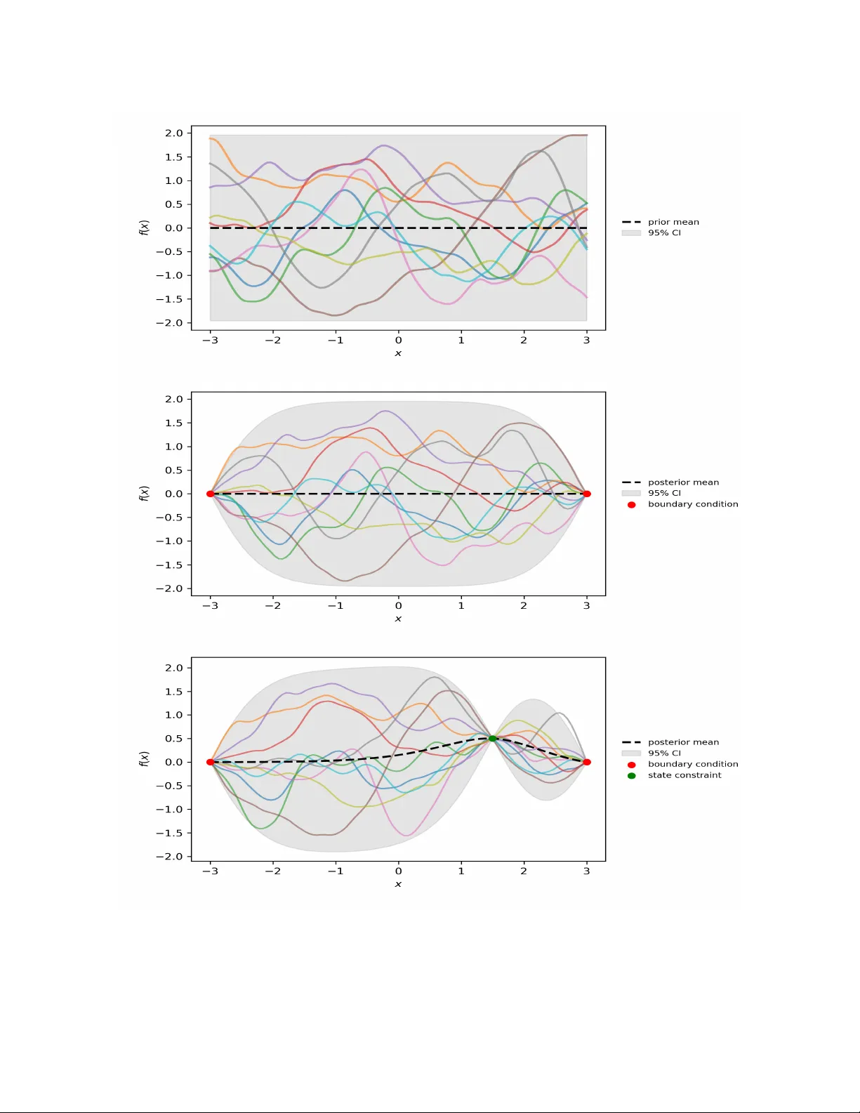
A Consensus-based optimization algorithm using Gaussian pro cesses for global optimization problems in Sob olev spaces Mahmoud Khatab ∗ and Claudia T otzec k † Marc h 17, 2026 Abstract W e prop ose an algorithm to approximate solutions of global optimization problems in Sob olev spaces that follo ws the spirit of Consensus-based algorithms in finite dimensions. The main in- gredien t are Gaussian pro cesses. In fact, w e exploit their ric h to olbox in order to dra w sample functions from Sob olev spaces that satisfy initial v alues, b oundary conditions or state constrain ts. W ell-known marginalization prop erties of Gaussian pro cesses help us to discretize the algorithm, that is stated in infinite dimensions, appropriately . W e illustrate the p erformance of the al- gorithm and show its feasibility for nonlinear b oundary v alue problems with state constrain ts as well as nonlinear optimal con trol problems constrained by a system of ordinary differential equations with sev eral numerical results. 1 In tro duction Ab out one decade ago the Consensus-based optimization (CBO) method for nonconv ex contin uous optimization problems in R d w as prop osed in [ 11 , 32 ]. Since then the metho d has attracted many researc hers from differen t bac kgrounds to push the limits in the theory of pro v ably conv ergen t metho ds for global optimization and to extend the range of application of such metho ds. Let us men tion some recen t con tributions that originate from v arious mathematical disciplines, i.e., the analysis of partial differential equations [ 5 , 18 , 20 , 26 ], in particular mean-field theory [ 2 , 21 , 30 ], sto c hastic analysis [ 4 , 22 ] or mathematical machine learning [ 13 ]. Also the range of applications that ma y be tackled with CBO-based tec hniques w as extended, see [ 8 , 9 , 14 , 15 , 17 , 36 ], and more robust versions were prop osed [ 19 , 27 ]. F or a quick start into co ding the metho d w e recommend the soft w are pack age [ 1 ]. Although the approac h presented below uses different tec hniques, the article aligns with recent adv ances tow ards global optimization in infinite dimensions. In particular, we w an t to mention: the multi-grid finite element approach combined with CBO for the constrained p -Allen-Cahn problem with obstacle [ 3 ]; the CBO approach for global optimization in the space of Gaussian probability measures [ 6 ]; the multiscale approac h for multi-lev el optimization with CBO [ 24 ]; and the mo del predictiv e control approach enhanced b y CBO [ 7 ]. The main contribution of the presen t article is the extension of Consensus-based optimization in the direction of global optimization problems in function spaces, that is, to infinite dimensional prob- lems. In particular, we consider Sobolev Spaces with elemen ts that may b e represented by samples ∗ Univ ersity of W upp ertal, Germany , khatab@uni-wupp ertal.de † Univ ersity of W upp ertal, Germany , totzeck@uni-wuppertal.de 1 from Gaussian pro cesses. W e remark that in general, the well-posedness analysis of optimization problems in function spaces exploits properties such as co ercivit y and w eakly lo w er semicon tin uit y of the ob jective functional and weak compactness arguments [ 25 ]. The pro ofs are therefore not con- structiv e and first-order optimality conditions are typically used to characterize solutions. Moreo v er, the first-order optimalit y conditions are the foundation to derive first-order optimization metho ds suc h as gradient descent. These are w ell-understo od, esp ecially in the case of Hilb ert spaces, and kno wn to globally conv erge to stationary p oin ts. How ever, additional assumptions, e.g. con v exit y , are required to deduce that stationary p oin ts are global minimizers. With the approach prop osed here we follo w a differen t av enue, instead of exploiting first-order conditions, we increase the num b er of function ev aluations and prop ose a zero-order metho d that aims to approximate the global minim um directly . In fact, we use Gaussian processes to randomly generate Sob olev functions and therefore to translate the exploration and exploitation of Consensus- based dynamics from finite dimensions to the Sob olev case. This allows us to form ulate a algorithm directly in the function space. Moreov er, the well-estab lished to olbox for Gaussian pro cesses can b e exploited to derive easy-to-implemen t algorithms as w e will show with the help of numerical sim ulation results for ODE- and PDE-b oundary v alue problems as well as optimal control problems constrained by nonlinear in teracting particle systems. Before jumping in to the details, we state the problem considered and sk etch the main idea that is further explained in the following sections. 1.1 Problem form ulation Let U be a function space with elemen ts that can b e represented as sample path of measurable Gaussian pro cess (GP) and f : U → R a p ossibly nonconv ex functional with unique global minimizer in U . W e are in terested in the global optimization problem min u ∈U f ( u ) . (1) F or instance, U can b e a Sobolev space of in teger order W m,p ( D ) , m ∈ N 0 , 1 < p < + ∞ , where D is an arbitrary op en set [ 23 ]. In particular, we are interested in the case p = 2 , where the Hilb ert structure allows for a direct relation of functions in the repro ducing kernel Hilb ert space H k of a giv en ke rnel k and their equiv alence class in H m ( D ) . The key element, whic h relates the state space U of the optimization problem with the GP is the kernel k also kno wn as co v ariance function. 1.2 Sk etch of the main idea In contrast to the usual use of GP in machine learning [ 33 ], GP are used in the following to sample functions with required smo othness to lift b oth, the diffusive part of the CBO dynamics and the initial conditions to the function space setting. Indeed, let GP 1 and GP 2 b e Gaussian pro cesses with sp ecific prop erties that we define later. F urther, let the time step size τ > 0 and drift parameter λ > 0 b e given. T o approximate the global solution of ( 1 ), we prop ose the time-discrete dynamics dU i j +1 = − λ ( U i j − v α f ( U j )) τ + √ 2 τ ∥ U i j − v α f ( U j ) ∥ U ξ i j , (2a) U i 0 ∼ GP 1 , ξ i j ∼ GP 2 , i = 1 , . . . , N , j = 0 , . . . , J, (2b) where v α f ( U j ) is the w eighted mean, computed in the usual spirit of Consensus-based metho ds [ 32 ] v α f ( U j ) = P N i =1 U i j e − αf ( U i j ) P N i =1 e − αf ( U i j ) , α ≫ 0 . 2 The similarity to the dynamics in the finite dimensional setting is obvious. The key idea leading to the formulation of the dynamics in ( 2 ) is strongly related to the interpretation of a GP as a distribution ov er functions. Indeed, we exp ect ξ i j to mimic the Brownian incremen ts of the finite dimensional sc heme. The t wo Gaussian pro cesses GP 1 and GP 2 pla y a crucial role and hav e to b e tailored for each state space U , that is eac h application individually . T o gain further insigh ts, we recall some c haracteristics of the GP in the next section. 2 Compilation of prop erties of Gaussian Pro cesses In this section w e recall some definitions in the con text of GP and related properties that are crucial for the prop osed algorithm. F rom the theoretical p oin t of view a particular fo cus lies on the relationship of the kernel function and the smo othness of the sample path, and from a numerical p oin t of view on the marginalization prop ert y . The latter pla ys a crucial role for the space discretization of ( 2 ) and is hea vily exploited in the implemen tation of our algorithm. W e closely follow [ 23 ]. 2.1 Basic definitions Let (Ω , F , P ) denote a probability space. Definition 1. The law P X of a r andom variable X : Ω → R is the pushforwar d me asur e of P thr ough X define d by P X ( B ) := P ( X − 1 ( B )) for al l Bor el sets B ∈ B ( R ) . Definition 2. A Gaussian pr o c ess  U ( x )  x ∈D is a family of Gaussian r andom variables define d over (Ω , F , P ) such that for al l n ∈ N , ( a 1 , . . . , a n ) ∈ R n and ( x 1 , . . . , x n ) ∈ D , P n i =1 a i U ( x i ) is a Gaussian r andom variable. Similar to the Gaussian distribution in finite dimensions, the law the GP induces ov er the function space R D endo w ed with its pro duct σ -algebra is uniquely determined by its mean and cov ariance functions m ( x ) = E [ U ( x )] and k ( x, x ′ ) = Co v ( U ( x ) , U ( x ′ )) . This allows us to write ( U ( x )) x ∈D ∼ GP ( m, k ) . The cov ariance function is often called k ernel in the literature, in this article the terms are used synonymously . The cov ariance function k is p ositiv e definite ov er D , i.e., for all n ∈ N ≥ 0 and ( x 1 , . . . , x n ) ∈ D n the matrix  k ( x i , x j )  1 ≤ i,j ≤ n is p ositiv e semidefinite. Con v ersely , for a giv en p ositiv e definite function ov er an arbitrary set D , there exists a centered GP indexed by D with this function as its cov ariance function. F or giv en ω ∈ Ω , the sample path U ω : D → R is the deterministic function U ω ( x ) := U ( x )( ω ) . 2.2 Kernel functions In the following we recall some kernel functions whic h are p opular in machine learning. F or more details and other classes of k ernel functions we refer to [ 33 ]. Squared Exp onen tial The squared exponential co v ariance function has the form k se ( r ) = exp  − r 2 2 ℓ 2  with parameter ℓ defining the characteristic length-scale. It is infinitely differen tiable, which means that the corresp onding GP has mean square deriv ativ es of all orders and th us is v ery smooth. Although, it is the most widely-used kernel within the k ernel mac hine fields, its strong smo othness assumptions are unrealistic for many ph ysical applications. 3 Matérn class The Matérn class of co v ariance functions is given b y k M ( r ) = 2 1 − ν Γ( ν ) √ 2 ν r ℓ ! ν K ν √ 2 ν r ℓ ! , where ℓ is again the length scale parameter, ν allo ws to controls the smo othness of the function, K ν is the mo dified Bessel function of the second kind and Γ( ν ) is the Gamma function. Note that for ν → ∞ we reco ver the squared exp onen tial kernel. The pro cess corresp onding to the Matérn class is m -times mean squared differentiable if and only if ν > m . Note that the k ernel b ecomes esp ecially simple if ν = p + 1 / 2 for a nonnegativ e integer p . Moreo ver, setting ν = 1 / 2 yields the exp onen tial kernel which yields a Gaussian pro cess that is mean squared contin uous but not mean squared differentiable. In one dimension, we obtain the Ornstein-Uhlenbeck pro cess with was in tro duced as a mathematical mo del of the v elo cit y of a particle undergoing Brownian motion. Remark. F or the numerics k M ( r ) is multiplie d by the signal varianc e σ 2 . This is an additional p ar ameter al lowing to adjust the amplitude of the functions gener ate d by the GP. 2.3 Smo othness of sample paths An o v erview of recent literature on the smo othness of sample path is given in the introduction of [ 23 ]. Moreov er, a very general result on the sample path Banach-Sobolev regularit y for Gaussian pro cesses can b e found in Prop osition 3.1 in this article, and a result on Hilb ert-Sc hmidt imbeddings of Sob olev spaces related to GPs is giv en in its Prop osition 4.4. The most relev ant result for the applications we hav e in mind is stated in Example 4.5 of the same article: If D is sufficiently smo oth, sample paths of a GP corresp onding to a Matérn kernel of order ν lie in H m ( D ) for m ∈ [0 , ν ) ∩ N 0 . Indeed, choosing ν = 3 / 2 or ν = 5 / 2 , which seem to b e the most relev ant cases in machine learning [ 33 ], yields sample paths of regularity H 1 ( D ) or H 2 ( D ) , resp ectiv ely . In addition, it is shown in [ 35 ] that in these cases the repro ducing kernel Hilb ert spaces (RKHS) coincide with H 1 ( D ) or H 2 ( D ) , resp ectiv ely . How ev er, in general the sample paths of a GP with k ernel k do not lie in the RKHS corresp onding to the same kernel. F or more details and results showing that the sample paths lie in an RKHS corresponding to a p ow er of that kernel in sp ecial cases, w e refer to [ 28 ]. 2.4 Marginalization and prediction The discussion ab o ve shows that sampling from a GP prior with appropriate parameters yields functions in Sob olev spaces. T o b e well-posed, optimization problems in Sob olev spaces usually in v olv e initial v alue or b oundary conditions. W e incorporate these with the help of an tailored p osterior. Moreov er, w e exploit the marginalization property which originates from the consistency requiremen t of GP for the numerical implementation of our scheme. F or further details on b oth, we refer to [ 33 ]. The main point is easy to see in finite dimensions: if the GP sp ecifies ( y 1 , y 2 ) ∼ N ( µ, Σ) for µ =  a b  ∈ R n 1 + n 2 and Σ =  A B B T C  ∈ R ( n 1 + n 2 ) × ( n 1 + n 2 ) then it holds y 1 ∼ N ( a, Σ 11 ) and y 2 ∼ N ( b, Σ 22 ) , resp ectiv ely . This ev en holds if y 2 con tains infinitely many v ariables, i.e., w e can compute the lik eliho od of y 1 under the join t distribution while ignoring y 2 . This helps us particularly in the implemen tation, since w e can compute finite dimensional pro jections of the underlying infinite ob ject on our computer. Indeed, we will represen t 4 the functions (sample paths of the GP) b y their finite dimensional pro jections which will correspond to the ev aluations on a predefined mesh. Similarly , we will handle given initial or b oundary data, and if applicable also state constraints, sp ecified by the application at hand. In fact, we split the v ariables into thee parts ( y 1 , y 2 , y 3 ) , where y 1 are the pro jections as ab ov e, y 2 con tains information given at data p oin ts and y 3 is infinite dimensional. As ab ov e y 3 can b e ignored in the computation. In order to incorp orate the data of y 2 in the finite pro jection y 1 , w e emplo y Ba y es rule as it is usually done when GP are used for predictions p ( y 1 | y 2 ) = p ( y 1 , y 2 ) p ( y 2 ) . Since we are in the Gaussian setting, w e can compute explicitly p ( y 1 | y 2 ) = N ( a + B C − 1 ( y 2 − b ) , A − B C − 1 B ⊤ ) , (3) where we used the notation from ab ov e. It is common to choose mean zero, that is, a and b zero v ectors [ 33 ] and we will do so in the following. A visualization of samples from the prior, samples from the p osterior with b oundary conditions and samples from the p osterior with additional state constrain ts are sho wn in Figure 1 . The shaded area sho ws the confidence band whic h is computed p oin twise b y adding the mean and t w o time the standard deviation at every p osition. 3 Algorithm and implemen tation W e note that the dynamics proposed in ( 2 ) is discrete in time but contin uous in space. Indeed, X i j is a function from some Sob olev space for eac h j and each i . T o obtain a sc heme that is feasible for implemen tation, we exploit the w ell-known marginalization prop erty , see Section 2.4 . 3.1 Algorithm in function space Let us denote b y GP ( m, k , θ ) the Gaussian Pro cess with mean m , kernel k and additional parameters θ , i.e., θ = ( ℓ, ν ) in case of the Matérn class. Moreov er, let us enco de initial v alue, boundary condi- tions or additional constraints with the help of an op erator c ( u ) = 0 . F or notational conv enience, we denote b y GP c ( m, k , θ ) the p osterior set. In more detail, U ∈ GP c ( m, k , θ ) is from the same space as GP ( m, k , θ ) with the additional prop ert y c ( U ) = 0 , that means, that initial v alue conditions, b oundary conditions and additional constraints are satisfied. F or notational conv enience, w e define the set GP 0 ( n, k , θ ) as p osterior set, where all constraints are assumed to b e homogeneous. F or example, if U ∼ GP c ( m, k , θ ) satisfies an initial condition U ( t 0 ) = ¯ u  = 0 , a sample ξ ∼ GP 0 ( m, k , θ ) w ould satisfy ξ ( t 0 ) = 0 . In every iteration of the algorithm w e consider the up date U i ← U i − λ ( U i − v α f ( U )) τ + √ 2 τ ∥ U i − v α f ( U ) ∥ U ξ i , U 0 ∈ GP c ( m, k , θ ) , ξ i ∈ GP 0 ( m, k , θ ) . Since v α f is a w eigh ted mean, the difference U i − v α f ( U ) satisfies homogeneous conditions. By defi- nition, ξ i satisfies homogeneous conditions. Altogether, this ensures that the initial, b oundary and additional conditions of the respective problem are met by eac h iterate of the algorithm, moreov er, that the regularit y of the functions is preserv ed in every iteration. F or more details on the up date pro cedure w e refer to Algorithm 1 . 5 Figure 1: Visualization of samples drawn from the GP defined via Matérn Kernel with parameters ν = 2 . 5 , ℓ = 1 and signal v ariance σ 2 = 1 . The shaded areas indicate the 95% confidence band. T op: 10 samples drawn from prior. Middle: 10 samples dra wn from p osterior which takes the b oundary conditions at x = − 3 and x = 3 into accoun t. Bottom: Visualization of 10 samples drawn from the GP with additional state constrain ts. 6 Algorithm 1 GP-CBO Require: n umber of CBO agents N ; constrain t p osterior GP c ( m, k , θ ) ; homogeneous posterior GP 0 ( m, k , θ ) ; time horizon T , time step size τ ; weigh t parameter α , drift parameter λ ; 1: J ← int ( T /τ ) 2: U 0 = ( U i ) i ← N indep endent samples U i ∼ GP c ( m, k , θ ) 3: for j = 0 , . . . J − 1 do 4: ev aluate v α f ( U j ) 5: ξ = ( ξ i ) i ← N indep endent samples ξ i ∼ GP 0 ( m, k , θ ) 6: compute the w eighed mean v α f ( U j ) 7: for i = 1 , . . . N do 8: U i j +1 ← U i j − λ ( U i j − v α f ( U j )) τ + √ 2 τ ∥ U i j − v α f ( U j ) ∥ U ξ i j 9: end for 10: end for 11: return v α f ( U J ) , U J W e wan t to emphasize that, by construction of GP c , giv en data, that is, state constraints, initial conditions or b oundary conditions are included in U . If we consider, for example, an initial v alue problem given b y d dt u = g ( u ) , u ( t 0 ) = u 0 . W e could apply Algorithm 1 with cost functional f ( u ) = ∥ d dt u − g ( u ) ∥ 2 L 2 (0 ,T ) and admissible set U = { u ∈ H 1 (0 , T ) : u ( t 0 ) = u 0 } . Cho osing appropriate parameters for the GP and sampling from the p osterior GP c then ensures that the samples U 0 satisfy U 0 ∈ U . Remark. (Isotropic versus anisotropic noise) R e c ent articles on CBO variants in finite dimensions discuss two differ ent typ es of noise terms: isotr opic given by | x − v f | dB i t and anisotr opic diag ( x − v f ) dB i t as first pr op ose d in [ 12 ]. In the function sp ac e setting, the isotr opic c ase tr anslates to the noise intr o duc e d ab ove, and the anisotr opic noise c orr esp onds to p ointwise multiplic ation of the functions ( U i j − v α f ( U j )) ξ i j . Noting that the p ointwise multiplic ation may le ad to loss of r e gularity (for example for f , g ∈ L 2 , in gener al f g / ∈ L 2 ), we chose the isotr opic c ase. This choic e is further underpinne d by numeric al simulations we r an, which showe d slower or even pr ematur e c onver genc e for the algorithm with p ointwise multiplic ation in the noise term. 3.2 Discretization and implemen tation Eac h U j in Algorithm 1 is a N -dimensional vector of samples from GP c ( m, k , θ ) , in particular, each U i j is a function. T o obtain an implementable version, we need to discretize these functions. Let therefore X = ( x p ) p ∈P b e a discretization of the domain of U i j , where P denotes the corresp onding index set that dep ends on the spatial dimension of the domain. Ev aluating the mean m and the k ernel k along X , w e obtain tensors m |X and k |X . In the particular case where the domain of the function is an interv al discretized with P ∈ N p oin ts, w e obtain P = { 1 , . . . , P } , whic h yields m |X = ( m ( x p )) p ∈ R P , k |X = ( k ( x p , x q )) p,q ∈ R P × P . 7 Let V ∼ GP ( m, k ) a sample path of the prior. A discretization of V is a multiv ariate Gaussian random v ariable v ∼ N ( m |X , k |X + σ 2 GP I ) , where I denotes the identit y matrix and σ 2 GP is a noise parameter of the Gaussian pro cess. Figure 1 (top) illustrates 10 samples v from the prior. T o include initial v alues, b oundary conditions or state state constraints, w e compute the corre- sp onding p osterior distribution with the help of Bay es rule. Since the initial data, b oundary data and state constrain ts are known information, these pla y the role of training p oints in the usual setting of GPs. T o discuss the details, we denote by x in the p oin ts where initial data are pre- scrib ed, x bc the p oin ts with prescrib ed b oundary conditions and x sc the p oin ts at which we hav e state constraints. F or notational con v enience we discuss the case where all types of conditions are presen t. If one case does not apply , we assume the corresp onding v ectors to be empty . The v ector x train = ( x in , x bc , x sc ) ∈ R d data collects all the giv en data in a vector of the dimension d data . No w, we build the matrices needed for the computation of the p osterior as follo ws A := k |X + σ 2 GP I ∈ R P × P , B = k |X ,x train ∈ R P × d data , C := k | x train ∈ R d data × d data , b y pairwise ev aluation of the kernel with the resp ectiv e p oin ts. Note that A corresp onds to the co v ariance matrix we already constructed for the prior. In B w e assemble the v alues combining the information of mesh and training p oin ts. And C collects the ev aluations of the training p oin ts. The distribution of the p osterior is then given by ( 3 ), hence in line 2 of Algorithm 1 w e dra w random v ariables U i ∼ GP c ( m, k , θ ) = N ( B C − 1 x train , A − B C − 1 B ⊤ ) . T o preserve the prescrib ed data in all iterations, we mak e sure that the up dates in line 5 of Algo- rithm 1 are set to zero at all training p oin ts, in more details the random v ariables satisfy ξ i ∼ GP 0 ( m, k , θ ) = N (0 , A − B C − 1 B ⊤ ) . 4 Applications The algorithm sp ecified in the previous section can b e used in very general settings. In the follo wing w e illustrate its p erformance with the help of b oundary v alue problems with state constraints and nonlinear optimal con trol problems constrained by ordinary differential equations. 4.1 Boundary v alue problems (BVP) Since unconstrained BVP are well-understoo d and in sp ecial cases ev en admit analytic solutions, we c ho ose them for the first tests of the prop osed algorithm. Indeed, we consider problems of the form e ( u ) = 0 , where the op erator e : U → Z may inv olve deriv atives of u and optional state constrain ts. T o guarantee w ell-p osedness, b oundary v alues ha v e to b e sp ecified. Most common are b oundary conditions of Dirichlet, Neumann or Robin-t yp e, w e use Dirichlet conditions in the follo wing as they are the simplest case to realize with the help of GP . As the constraints are incorporated in the p osterior distribution, w e are free to choose an appropriate cost functional without explicitly addressing the constrain ts. Therefore a candidate for an appropriate cost functional is giv en b y f ( u ) = ∥ e ( u ) ∥ 2 Z F or example, Z = L 2 ( D ) yields f ( u ) = R D e ( u ) 2 dx . 8 Remark. F or BVP which al low for the wel l-p ose dness analysis b ase d on ener gy estimates, the ener gy functional may b e use d as alternative c ost functional. Note that these usual ly r e quir e less r e gularity and henc e less derivatives of u have to b e c ompute d to evaluate the c ost functional. 4.2 Optimization problems constrained b y differen tial equations The second class of problems w e consider are global optimal con trol problems. W e think of con- strain ts given by ordinary differential equations (ODE) or partial differen tial equations (PDE) which often arise in ph ysics. In more detail, we consider problems of the form min y ∈Y ,u ∈U J ( y , u ) sub ject to e ( y , u ) = 0 , (OC) where J : Y × U → R is a cost functional and the op erator e : Y × U → Z encodes the state constrain t. In more detail e ( y , u ) = 0 implies that y is the solution of the differential equation for giv en control u . Assuming the well-posedness of the state equation, it is common practice to in tro duce the con trol-to-state map S : U → Y . If y = S ( u ) , we in tro duce the reduced cost functional f ( u ) := J ( S ( u ) , u ) . Then ( OC ) problem can b e rewritten as min u ∈U f ( u ) . Hence, instead of considering the constrain t explicitly , it is taken into accoun t via S . How ever, w e are now in an unconstrained setting and ma y apply Algorithm 1 . Remark. Existenc e r esults for ( OC ) ar e usual ly b ase d on c o er civity of J w.r.t. u , we ak c ontinuity and b ounde dness of the map S and we akly lower semic ontinuity of J . The ar guments ar e ther efor e not c onstructive and often first-or der optimality c onditions ar e use d to char acterize and c ompute lo c al minimizers. W e r efer to [ 25 ] for mor e details. In c ontr ast, A lgorithm 1 is a zer o-or der metho d that aims to appr oximate the glob al solution of ( OC ) . This is p articularly of inter est if the c onstr aints or the c ost functional ar e nonline ar, sinc e this c auses usual ly nonc onvexity and ther efor e lo c al and glob al solutions may differ. 5 Numerical results In the follo wing w e sho w n umerical results for the differen t problem classes discussed in Section 4 . W e b egin with b oundary v alue problems. F or the n umerical computations we used the Matérn k ernel with length scale ℓ = 1 and smo othness parameter ν = 2 . 5 if not stated otherwise. The code used for the n umerical results is av ailable here [ 29 ]. 5.1 Boundary v alue problems First, w e test our approac h in one and tw o dimensional settings with b oundary v alue problems that admit exact solutions. Then w e add some state constraints, which p ose a may or c hallenge for standard solution methods and justify the additional computational effort of the CBO approac h. 9 5.1.1 One dimensional case Indeed, we consider the follo wing boundary v alue problem [ 34 ]: u ′′ ( x ) + u ( x ) = 0 (4) with the boundary conditions u (0) = 0 , u  π 2  = 2 . (5) In the CBO approac h w e measure feasibility of a candidate function u via the residual of the differen tial equation and use the cost functional f ( u ) = Z π / 2 0  u ′′ ( x ) + u ( x )  2 dx, (6) where the b oundary conditions are enforced b y sampling from a Gaussian pro cess posterior condi- tioned on u (0) = 0 and u ( π / 2) = 2 . The exact solution is given by u ∗ = 2 sin( x ) . (7) T o quantify the difference betw een the CBO solution u and the exact solution u ∗ , we consider the error function e ( x ) = u ( x ) − u ∗ ( x ) . (8) W e measure this error in the L 2 -norm and L ∞ -norm, resp ectiv ely defined b y ∥ e ∥ L 2 (Ω) :=  Z Ω | e ( x ) | 2 dx  1 / 2 , ∥ e ∥ L ∞ (Ω) := sup x ∈ Ω | e ( x ) | , (9) where Ω = [0 , π / 2] . During the CBO iterations, w e monitor the evolution of the cost functional and the error norms. Figure 2 summarizes the conv ergence b eha vior: the left panel sho ws the decay of the cost functional J ( u ) o ver the iterations, while the righ t panel presen ts the ev olution of the L 2 - and L ∞ -norms of the error e ( x ) . (a) Cost functional J ( u ) (b) Error norms ∥ e ∥ L 2 (Ω) and ∥ e ∥ L ∞ (Ω) Figure 2: Evolution of the cost functional and the error norms during the CBO iterations. 10 Figure 3: Comparison b et ween unconstrained and constrained solution found by CBO. No w, we consider the problem with additional state constraints at t w o p oin ts on the mesh x 1 = 1 . 189997 with y ( x 1 ) = 1 . 85673 , x 2 = 1 . 20586 with y ( x 2 ) = 1 . 86829 . Due to the additional constraints the problem, we do not hav e analytical solution, how ever w e see in Figure 3 that the solution found by CBO b ehav es similar to the unconstrained case. 5.1.2 T w o dimensional case W e extend our tests to 2d to solv e the following Poisson problem: − ∆ u ( x, y ) = − 6 , ( x, y ) ∈ Ω , (10a) u ( x, y ) = 1 + x 2 + 2 y 2 , ( x, y ) ∈ ∂ Ω , (10b) Ω = [0 , 1] × [0 , 1] . (10c) The exact solution of problem ( 10 ) is u e ( x, y ) = 1 + x 2 + 2 y 2 . (11) The computational domain Ω = [0 , 1] × [0 , 1] is discretized by a uniform structured grid with N x = N y = 30 no des in eac h spatial direction. The numerical solution obtained b y CBO is compared with the analytical solution in Figure 4 . Figure 4: Comparison b et ween the CBO solution and the analytical solution for the tw o- dimensional Poisson problem ( 10 ). 11 In the CBO approach, feasibility of a candidate function u is measured via the residual of the P oisson equation, and we use the cost functional J ( u ) = Z Ω  ∆ u ( x, y ) − 6  2 dx dy , (12) where ∆ u = u xx + u y y and Ω = [0 , 1] × [0 , 1] . T o quantify the difference b etw een the CBO solution u and the exact solution u e , we define the error function e ( x, y ) = u ( x, y ) − u e ( x, y ) , (13) and measure it in the L 2 -norm and L ∞ -norm, resp ectiv ely , ∥ e ∥ L 2 (Ω) :=  Z Ω | e ( x, y ) | 2 dx dy  1 / 2 , ∥ e ∥ L ∞ (Ω) := sup ( x,y ) ∈ Ω | e ( x, y ) | . (14) During the CBO iterations, we monitor the evolution of the cost functional and the error norms, sho wn in Figure 5 : the left panel displays the cost J ( u ) o v er the iterations, while the righ t panel rep orts the evolution of ∥ e ∥ L 2 (Ω) and ∥ e ∥ L ∞ (Ω) . (a) Cost functional J ( u ) (b) Error norms ∥ e ∥ L 2 (Ω) and ∥ e ∥ L ∞ (Ω) Figure 5: Evolution of the cost functional and the error norms during the CBO iterations for the tw o-dimensional Poisson problem ( 10 ). No w, we consider the problem with additional state constraints at four p oin ts on the mesh ( x 1 , y 1 ) = (0 . 72413793 , 0 . 72413793) , ( x 2 , y 2 ) = (0 . 75862069 , 0 . 72413793) , ( x 3 , y 3 ) = (0 . 72413793 , 0 . 75862069) , ( x 4 , y 4 ) = (0 . 75862069 , 0 . 75862069) , with prescrib ed v alues u ( x 1 , y 1 ) = 2 . 31581451 , u ( x 2 , y 2 ) = 2 . 36183115 , u ( x 3 , y 3 ) = 2 . 40784780 , u ( x 4 , y 4 ) = 2 . 45386445 . Due to the additional state constraints, we do not hav e an analytical solution for the constrained problem. Instead, we compare the absolute difference abs_diff ( x, y ) =   u CBO ( x, y ) − u exact ( x, y )   12 for the unconstrained and constrained cases, depicted in Figure 6 in the form of heat maps. (a) Unconstrained case: heat map of | u CBO − u exact | . (b) Constrained case: heat map of | u CBO − u exact | . Figure 6: Comparison of the absolute error | u CBO − u exact | betw een the unconstrained and constrained CBO solutions for the tw o-dimensional Poisson problem ( 10 ). W e use the same color bar range in Figures 6 (a) and 6 (b) in order to ensure a fair comparison b et ween the tw o configurations, which do es not mean that the heat map in Figure 6 (a) is identically zero ev erywhere. T o further illustrate that the unconstrained CBO solution is not exactly equal to the analytical one, w e also plot the signed difference diff ( x, y ) = u CBO ( x, y ) − u exact ( x, y ) for the unconstrained case; see Figure 7 . This plot rev eals small but nonzero deviations across the domain, which are to o small to b e clearly visible when using the shared color scale in Figure 6 . Figure 7: Signed difference diff ( x, y ) = u CBO ( x, y ) − u exact ( x, y ) for the unconstrained P oisson problem ( 10 ). W e study the p erformance of CBO on a more complex problem, namely a tw o-dimensional nonlinear example. In order to obtain an analytical solution for comparison, w e mak e use of the 13 metho d of manufactur e d solutions , as describ ed in [ 31 ]. Hence we adapt problem ( 10 ) to the nonlinear equation − ∆ u + u 3 = f ( x, y ) , ( x, y ) ∈ Ω , (15) where the source term is c hosen as f ( x, y ) = − 6 + (1 + x 2 + 2 y 2 ) 3 (16) and Dirichlet b oundary condition as in ( 10 ), namely u ( x, y ) = 1 + x 2 + 2 y 2 on ∂ Ω . By construction, w e obtain the same exact solution as in ( 11 ), u e ( x, y ) = 1 + x 2 + 2 y 2 . The output of the nonlinear CBO solution compared to the exact solution is shown in Figure 8 . During the CBO iterations, w e monitor the evolution of the cost functional and the error norms, sho wn in Figure 9 : the left panel displays the cost J ( u ) o v er the iterations, while the righ t panel rep orts the evolution of ∥ e ∥ L 2 (Ω) and ∥ e ∥ L ∞ (Ω) . W e can see that the p erformance of CBO w as not influenced b y the increased complexity of the nonlinear example, since for CBO this corresp onds only to a small modification of the cost functional. This highlights another adv antage of the CBO approac h. Figure 8: Comparison b et ween the CBO solution for ( 15 ) and the exact solution. (a) Cost functional J ( u ) (b) Error norms ∥ e ∥ L 2 (Ω) and ∥ e ∥ L ∞ (Ω) Figure 9: Evolution of the cost functional and the error norms during the CBO iterations for the tw o-dimensional nonlinear problem ( 15 ). 14 5.2 Optimal con trol problems In this section we consider an optimal control problem constrained by a nonlinear nonlo cal ODE, whic h mo dels an interaction of sheep and shepherd dogs. Due to the nonconv exity induced by the nonlinear in teractions, we expect to hav e lo cal and global minima. The problem w e discuss in the follo wing was already considered in [ 10 ] and a gradient descent (GD) algorithm was deriv ed and used for numerical results. Of course, using a gradient approac h we can only hop e to con ve rgence to lo cal minima, while w e aim for global solutions here. 5.2.1 Mathematical form ulation of the shepherd problem W e no w consider an optimal con trol problem that aims to gather the sheep close to a predefined destination p oin t x des ∈ R 2 and therefore define the cost functional based on the v ariance and cen ter of mass of the sheep flo c k. In more detail, let N S ∈ N b e the num b er of sheep in the flo c k and x i , v i : [0 , T ] → R 2 denote the p osition and v elo cit y of the i -th sheep, resp ectiv ely . W e assume to b e able to control the v elo cit y of the dog u : [0 , T ] → R 2 . The interaction of the sheep flo c k and the shepherd dog are assumed to b e p oten tial based, hence by Newton’s Third La w w e obtain the dynamics d dt x i = v i , x i (0) = x 0 ,i , i = 1 , . . . , N S , (17a) d dt v i = − αv i − 1 N S N S X j =1 K s ( x j − x i ) − K d ( d − x i ) , v i (0) = v 0 ,i , (17b) d dt d = u, d (0) = d 0 , (17c) where K s and K d are the gradients of the interaction p oten tials mo deling binary sheep-sheep and sheep-dog interactions, resp ectiv ely . The parameter α > 0 causes damping. F or the n umerical implementation of the in teractions w e use the Morse p oten tial [ 16 ] P ( r ) = C r s/d exp  − | r | l r  − C a exp  − | r | l a  , K s/d ( r ) =  − C r l r exp  − | r | l r  + C a l a exp  − | r | l a  r | r | , where C r , l r are parameters for strength and range of the repulsion force, resp ectively , and C a , l a are parameters for strength and range of the attraction force, resp ectiv ely . W e adjust the forces of the sheep-sheep and sheep-dog in teractions by choosing different range and strength parameters. In order to mo del the task of gathering the sheep flo c k around the destination p oin t x des w e use the cost functional giv en by J = Z T 0 σ 1 ( V ( t ) − V 0 ) 2 + σ 2 ∥ E ( t ) − x des ∥ 2 + σ 3 ∥ u ( t ) ∥ 2 dt, where E ( t ) ∈ R D is the cen ter of mass of the sheep flock at time t defined as E ( t ) = 1 N S N S X i =1 x i ( t ) , and V ( t ) is the v ariance of the sheep flock p ositions at time t defined as V ( t ) = 1 N S N S X i =1 ∥ x i ( t ) − E ( t ) ∥ 2 . 15 Hence, the first in tegrand in the cost functions measures the deviation of flock’s v ariance from the prescrib ed target v ariance V 0 . The second integrand measures the distance of the center of mass of the flo c k to the desired destination. Both together aim to gather the crowd around x des . The third integrand has the physical meaning of minimizing the kinetic energy used for the task. Mathematically , it causes the cost functional to b e co erciv e w.r.t. u ∈ L 2 ((0 , T ) , R 2 ) . The w eights λ 1 , λ 2 , λ 3 ≥ 0 allo w us to adjust the influence of the differen t terms. T o hav e a regularit y that is comparable to L 2 ((0 , T )) , whic h is used for the gradient descent approach, we choose ν = 0 . 5 for the regularity parameter of GP . Assuming enough regularity for K s/d , and given u ∈ L 2 ((0 , T )) ( 17 ) admits a unique solution y ( u ) = ( x u , v u , d u ) . This allows us to define the reduced cost functional f ( u ) = J ( y ( u ) , u ) , whic h is used in the CBO algorithm. W e wan t to emphasize that for each ev aluation of f w e ha v e to solv e the ODE system ( 17 ). W e compare our results to the ones obtained by a gradien t descen t metho d (GD). The latter only requires one solve of ( 17 ) and its adjoint system in each gradien t step. How ever, it only guarantees to find stationary p oints. In our sp ecific case, the main optimization lo op was executed for 3000 iterations with 100 CBO agen ts, resulting in a total of 3000 × 100 = 300000 functional ev aluations. This is considerably more exp ensiv e compared to the gradient descen t metho d, whic h required only 2887 ev aluations for the step size search with Armijo rule and the up date. Despite the higher computational cost of CBO compared to GD, CBO achiev es a significant reduction of the ob jective functional. Indeed, w e ran the CBO algorithm with ν = 0 . 5 and ν = 2 . 5 five times eac h. F or ν = 0 . 5 the mean final total cost v alue is 2821 . 19 and for ν = 2 . 5 the mean final total cost v alue is 2840 . 94 while the GD w as stuck with a v alue of 3890 . 36 . A ccording to the theory on GP , with ν = 0 . 5 w e seek within functions of lo w er regularit y than for ν = 2 . 5 . Therefore the sligh t improv ement for ν = 0 . 5 is reasonable. The b est run for ν = 0 . 5 lead to nearly 30% reduction in the cost compared to GD while the mean of the fiv e runs of ν = 0 . 5 lead to ab out 27 . 48% reduction. The mean of the fiv e runs of ν = 2 . 5 lead to a reduction by 26 . 97% compared to GD. The cost ev olution ov er the iterations for b oth metho ds is presen ted in Figure 10 . In the left panel the CBO cost evolut ion for a certain run in case of ν = 0 . 5 is shown together with tw o dashed reference lines indicating the final total cost achiev ed b y CBO and the final total cost obtained b y GD. The righ t panel shows the cost evolution corresp onding to the GD method. The evolution of the sheep flo c k (blue circles) and the dogs (red triangles) under the optimized con trol for a v alue of ν = 0 . 5 is shown in Figure 11 . The sim ulation is p erformed with 100 sheep and 2 dogs, while the orange star indicates the target lo cation. 16 (a) CBO cost evolution for a certain run in case of ν = 0 . 5 with dashed reference lines indicating the final GD and CBO costs. (b) Cost evolution for the gradient descent (GD) metho d. Figure 10: Comparison of the cost ev olution ov er the iterations for CBO and GD. Figure 11: Snapshots of the sheep–dog dynamics under the optimized control for a certain run for v alue of ν = 0 . 5 . Blue circles represent the sheep flo c k, red triangles denote the dogs, and the orange star marks the target location. 6 Conclusion and outlo ok In this article w e hav e prop osed a zero-order optimization algorithm for general problems in Sob olev spaces. The main idea was to exploit the to olbox of Gaussian Pro cesses in order to sample functions with prescrib ed regularit y that additionally satisfy constraints at giv en p oin ts. The algorithm was tested in differen t settings inv olving b oundary v alue problems for ODE and PDE. Moreov er, we hav e sho wn that the metho d is able to significantly impro v e the solution found by first-order metho ds for a highly nonlinear optimal control problem constrained b y ODE. The promising results pro vided in this pap er motiv ate further researc h in v arious directions including the analysis of the prop osed algorithm in the discrete setting, the conv ergence tow ards a nonlinear system of SDE in Sob olev Space as τ → 0 . Moreov er, it is op en to chec k if the mean-field theory and in particular the global conv ergence pro of that was established for CBO dynamics in finite state spaces can b e generalized to the setting in Sob olev spaces as N → ∞ . 17 A c kno wledgement This research receiv ed funding by the German F ederal Ministry of Education and Research under the gran t num b er 05M22PXA. Responsibility for the con ten t of this publication lies with the authors. References [1] R. Bailo, A. Barbaro, S. N. Gomes, K. Riedl, T. Roith, C. T otzeck, and U. V aes. Cbx: Python and julia pack ages for consensus-based interacting particle metho ds. Journal of Op en Sour c e Softwar e , 9(98):6611, 2024. [2] A. Baldi. An alternativ e approac h to well-posedness of mc k ean-vlaso v equations arising in consensus-based optimization. arXiv pr eprint arXiv:2512.19446 , 2025. [3] J. Beddrich, E. Chenchene, M. F ornasier, H. Huang, and B. W ohlmuth. Constrained consensus- based optimization and n umerical heuristics for the few particle regime, 2026. [4] S. Bella via and G. Malaspina. A discrete consensus-based global optimization metho d with noisy ob jectiv e function. Journal of Optimization The ory and Applic ations , 206(1):20, 2025. [5] S. Bonandin, K. Riedl, and S. V eneruso. Strong global con vergence of the consensus-based optimization algorithm. arXiv pr eprint arXiv:2512.10654 , 2025. [6] G. Borghi and J. A. Carrillo. V ariational inference via gaussian interacting particles in the bures-w asserstein geometry . arXiv pr eprint arXiv:2601.00632 , 2026. [7] G. Borghi and M. Herty . Mo del predictiv e con trol strategies using consensus-based optimization. Mathematic al Contr ol and R elate d Fields , 15(3):876–894, 2025. [8] L. Bungert, F. Hoffmann, D. Kim, and T. Roith. Mirrorcb o: A consensus-based optimization metho d in the spirit of mirror descen t. arXiv pr eprint arXiv:2501.12189 , 2025. [9] L. Bungert, T. Roith, and P . W ack er. P olarized consensus-based dynamics for optimization and sampling. Mathematic al Pr o gr amming , 211(1):125–155, 2025. [10] M. Burger, R. Pinnau, C. T otzeck, O. T se, and A. Roth. Instantaneous con trol of in teracting particle systems in the mean-field limit. Journal of Computational Physics , 405:109181, 2019. [11] J. A. Carrillo, Y.-P . Choi, C. T otzeck, and O. T se. An analytical framework for consensus- based global optimization metho d. Mathematic al Mo dels and Metho ds in Applie d Scienc es , 28:1037–1066, 2018. [12] J. A. Carrillo, S. Jin, L. Li, and Y. Zhu. A consensus-based global optimization metho d for high dimensional machine learning problems. ESAIM: Contr ol, Optimisation and Calculus of V ariations , 27:S5, 2021. [13] J. A. Carrillo, N. G. T rillos, S. Li, and Y. Zhu. F edcb o: Reaching group consensus in clustered federated learning through consensus-based optimization. Journal of machine le arning r ese ar ch , 25(214):1–51, 2024. [14] E. Chenc hene, H. Huang, and J. Qiu. A consensus-based algorithm for non-con v ex m ultipla y er games. Journal of Optimization The ory and Applic ations , 206(2):45, 2025. 18 [15] R. J. de Keijzer, L. Y. Visser, O. T se, and S. J. Kokk elmans. Consensus-based qubit configura- tion optimization for v ariational algorithms on neutral atom quantum systems. npj Quantum Information , 11(1):186, 2025. [16] M. R. D’Orsogna, Y. Ch uang, and A. Bertozzi. Self-prop elled particles with soft-core interac- tions: patterns, stability and collapse. Physic al R eview L etters , 96(10):104302, 2006. [17] M. F ornasier and L. Sun. A p de framew ork of consensus-based optimization for ob jectiv es with m ultiple global minimizers. Communic ations in Partial Differ ential Equations , 50(4):493–541, 2025. [18] M. F ornasier and L. Sun. Regularity and p ositivit y of solutions of the consensus-based opti- mization equation: unconditional global conv ergence. arXiv pr eprint arXiv:2502.01434 , 2025. [19] N. García T rillos, A. Kumar Ak ash, S. Li, K. Riedl, and Y. Zhu. Defending against diverse at- tac ks in federated learning through consensus-based bi-level optimization. Philosophic al T r ans- actions of the R oyal So ciety A: Mathematic al, Physic al and Engine ering Scienc es , 383(2298), 2025. [20] N. Gerber, F. Hoffmann, D. Kim, and U. V aes. Uniform-in-time propagation of c haos for consensus-based optimization. arXiv pr eprint arXiv:2505.08669 , 2025. [21] N. J. Gerb er, F. Hoffmann, and U. V aes. Mean-field limits for consensus-based optimization and sampling. ESAIM: Contr ol, Optimisation and Calculus of V ariations , 31:74, 2025. [22] S. Góttlich, J. Heieck, and A. Neuenkirc h. Exp onen tial stability of finite- n consensus-based optimization. arXiv pr eprint arXiv:2510.19565 , 2025. [23] I. Henderson. Sob olev regularity of gaussian random fields. Journal of F unctional Analysis , 286:110241, 2024. [24] M. Herty , Y. Huang, D. Kalise, and H. K ouhkouh. A multiscale consensus-based algorithm for m ultilev el optimization. Mathematic al Mo dels and Metho ds in Applie d Scienc es , 35(10):2207– 2243, 2025. [25] M. Hinze, R. Pinnau, M. Ulbrich, and S. Ulbric h. Optimization with PDE Constr aints , v ol- ume 23 of Mathematic al Mo del ling: The ory and Applic ations . Springer-V erlag, 2009. [26] H. Huang, H. Kouhk ouh, and L. Sun. F aithful global conv ergence for the rescaled consensus- based optimization. arXiv pr eprint arXiv:2503.08578 , 2025. [27] Y. Huang, M. Herty , D. Kalise, and N. Kan tas. F ast and robust consensus-based optimization via optimal feedbac k con trol. SIAM Journal on Scientific Computing , 48(1):A74–A102, 2026. [28] M. Kanaga wa, P . Hennig, D. Sejdino vic, and B. K. Srip erumbudur. Gaussian pro cesses and k ernel metho ds: A review on connections and equiv alences, 2018. [29] M. Khatab and C. T otzec k. Implemen tation of the consensus-based optimization metho d using gaussian pro cesses. https://doi.org/10.5281/zenodo.19050573. [30] M. Koß, S. W eissmann, and J. Zec h. On the mean-field limit of consensus-based metho ds. Mathematic al Metho ds in the Applie d Scienc es , 2025. 19 [31] H. P . Langtangen and A. Logg. Solving PDEs in Python: The FEniCS T utorial V olume I . Springer, Cham, 2017. Released under CC A ttribution 4.0 license. [32] R. Pinnau, C. T otzeck, O. T se, and S. Martin. A consensus-based model for global optimization and its mean-field limit. Mathematic al Mo dels and Metho ds in Applie d Scienc es , 27:183–204, 2017. [33] C. E. Rasm ussen and C. K. I. Williams. Gaussian Pr o c esses for Machine L e arning . The MIT Press, 2006. [34] G. F. Simmons. Differ ential Equations with Applic ations and Historic al Notes . CR C Press, T aylor & F rancis Group, 3rd edition, 2017. [35] I. Steinw art. Conv ergence types and rates in generic Karhunen-Loeve expansions with applica- tions to sample path prop erties. Potential Analysis , 51(3):361–395, 2019. [36] X. Sun, A. Jordana, M. F ornasier, J. Etesami, and M. Khadiv. Consensus-based optimization (cb o): T o w ards global optimalit y in rob otics. arXiv pr eprint arXiv:2602.06868 , 2026. 20