On the CRLB for Blind Receiver I/Q Imbalance Estimation in OFDM Systems: Efficient Computation and Closed-Form Bounds

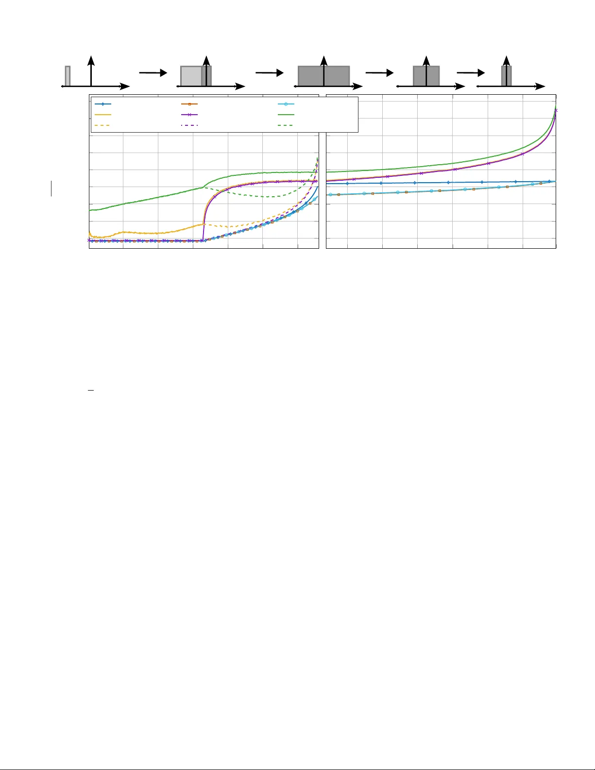
1 On the CRLB for Blind Recei v er I/Q Imbalance Estimation in OFDM Systems: Ef ficient Computation and Closed-F orm Bounds Moritz T ockner ∗ 1 , Oli ver Lang ∗ 2 , Andreas Meingassner -Lang ∗ 3 , Mario Huemer ∗ 4 ∗ Institute of Signal Processing, Johannes K epler Uni versity Linz, Austria { 1 moritz.tockner , 2 oli ver .lang, 3 andreas.meingassner -lang, 4 mario.huemer } @jku.at Abstract —Modern mobile communication receivers ar e often implemented with a direct-con version architectur e, which fea- tures a number of advantages over competing designs. A notable limitation of direct-con version ar chitectures, howe ver , is their sen- sitivity to amplitude and phase mismatches between the in-phase and quadrature signal paths. Such in-phase and quadrature- phase (I/Q) imbalances introduce undesired image components in the baseband signal, degrading link performance—most notably by incr easing the bit-err or ratio. Considerable resear ch effort has therefor e been devoted to digital techniques for estimating and mitigating these impairments. Existing approaches generally fall into two categories: data-aided methods that exploit kno wn pilots, preambles, or training sequences, and blind techniques that operate without such prior information. For data-aided estimation, Cram ´ er -Rao lower bounds (CRLBs) have been es- tablished in the literature. In contrast, the deriv ation of a CRLB for the blind I/Q-imbalance estimation case is considerably more challenging, since the recei ved data is random and typically non- Gaussian in the frequency domain. This work extends our earlier conference contribution, which introduced a CRLB derivation for the blind estimation of frequency-independent (FID) receiver I/Q imbalance using central limit theorem (CL T) arguments. The extensions include a computationally efficient method for calculating the bound, reducing complexity from cubic in the number of samples to linear in the fast-Fourier transform (FFT) size, along with a simplified closed-form approximation. This ap- proximation provides new insights into the allocation-dependent performances of existing estimation methods, motivating a pre- estimation filtering modification that drastically improves their estimation performance in certain scenarios. Index T erms —CRLB, direct-con version receiver , I/Q imbal- ance, OFDM I . I N T R O D U C T I O N The direct-con version or homodyne receiv er lends it- self to popularity in state-of-the-art mobile communication transceiv er designs due to multiple advantages compared to a classical heterodyne architecture [1]. It operates by splitting the received radio frequency (RF) signal into two paths: the in-phase and quadrature-phase path. Each path is subsequently downcon verted to the baseband using the local oscillator (LO) signal. Howe ver , due to e.g., manufacturing tolerances or component aging, the I/Q paths often exhibit unequal signal gains and a phase relation that deviates from the ideal 90 ◦ . This results in gain and phase mismatches (commonly referred to as I/Q imbalance) in the resulting complex baseband signal. These mismatches are typically assumed to be FID and lead to an unwanted image in the downcon verted signal spectrum. T ypically , analog filtering is implemented between the down- mixing and the analog-to-digital con verter (ADC), which also results in slight dif ferences between the I/Q paths. These lead to frequency-dependent (FD) imbalances, which are typically smaller in magnitude than the FID imbalances [2]–[4], and are not considered in this work. W e deri ve a CRLB for the blind estimation problem of an FID recei ver I/Q imbalance based on a general orthogonal frequency-di vision multiplexing (OFDM) downlink (DL) sig- nal model. The deriv ation applies to any cyclic-prefix (CP)- OFDM system, encompassing current standards such as 5G New Radio (NR) as well as future systems like 6G. The CRLB provides a useful reference for unbiased estimators, as it represents the minimum achiev able estimation variance of the unknown parameters [5]. For FID recei ver I/Q imbalance estimation, CRLBs are extensi vely inv estigated in literature. Ho we ver , in most studies either a training sequence or pilot subcarriers are required [6]–[12], which entails e xact kno wledge of specific receiv ed symbols at the receiv er . It also necessitates the estimation of other non-idealities distorting these kno wn symbols, such as carrier-frequency offset (CFO), phase-of fset or a fading channel. In this work, we consider a fully blind estimation approach without any knowledge of the receiv e signal, and deriv e the corresponding CRLB. Related literature includes [13]–[15]. In [13], the CRLB is deriv ed under a frequenc y-domain constant-modulus as- sumption on the transmitted symbols, used as prior knowl- edge, which restricts the applicability to quadrature phase-shift keying (QPSK) and binary phase-shift keying (BPSK). This assumption is fragile in practice, as frequency-selecti ve chan- nels impose frequenc y-dependent attenuation [16], thereby destroying the constant modulus property in the frequenc y domain. The formulation further requires joint estimation of I/Q imbalance and CFO. Moreover , [13] reports the CRLB as plotted curves and omits both, the deri vation, and the closed- form expression. This precludes a reproducible analytical com- parison. Furthermore, since the work relies on the constant- modulus assumption, which is misaligned with our general quadrature amplitude modulation (QAM)-based setting, and no closed-form expression is av ailable for comparison, we 2 exclude the CRLB of [13] from our comparison. [14] simplifies the CRLB deriv ation by including the transmitted symbols as additional parameters, making the bound data dependent. A data-independent bound can then be obtained through an ensemble av erage from multiple sim- ulation runs with random data, significantly increasing the simulation time. Additionally , the computational complexity per run scales cubically with the number of samples used for estimation. In contrast, our method requires no repeated simulations and can be optimized to a computational complex- ity independent of the number of processed OFDM symbols. Hence, it scales linearly with the FFT size. In [15], it is shown that for asymmetric subcarrier alloca- tions, the estimation bias of a specific, well-kno wn moment- based estimator (MBE) [17], [18] is limited solely by the white Gaussian noise (WGN) added after the imbalance, and by the imbalance itself. In contrast, we provide a similar but more general conclusion, showing via the CRLB that this result extends to the mean square error (MSE) of an y unbiased estimator . This paper is a substantially e xtended version of our foun- dational work presented at the 2025 Asilomar Conference on Signals, Systems, and Computers [19]. While the conference paper introduced the core CRLB deriv ation, this manuscript provides sev eral significant new contributions: (i) a computa- tionally efficient method for calculating the bound, reducing the computational complexity from cubic in the number of samples used for estimation, to linear in the FFT size; (ii) a simplified, closed-form approximation of the CRLB that yields deeper analytical insights into its dependency on the subcarrier allocation (in particular its symmetry), the number of OFDM symbols, and the signal-to-noise ratio (SNR); (iii) a nov el pre-estimation filtering technique to improve estimator performance in scenarios where the allocation consists of asymmetric and symmetric components; and (iv) a compre- hensiv e performance analysis across various SNR and image- leakage ratio (ILR) v alues. The remainder of this paper is or ganized as follo ws: Sec- tion II provides an overvie w of the typically used FID I/Q imbalance model. Section III presents the statistical signal model and its underlying assumptions, along with a justifi- cation for their v alidity , followed by the deriv ation of the CRLB, its optimized ev aluation, and a simplified closed-form approximation. In Section IV, the estimation performances of multiple state-of-the-art algorithms are e valuated, and their behavior for dif ferent simulation scenarios is compared to the CRLB. This section also demonstrates the ef fectiveness of the proposed pre-estimation filtering technique. Finally , Section V concludes the paper . I I . S I G N A L M O D E L In this paper , we adopt a baseband signal model analogous to the one presented in [20]. An overvie w of the k ey processing steps is pro vided in Fig. 1. A. Baseband Model In this work, we consider a general CP-OFDM DL signal model. A data source generates uniformly distributed random Fig. 1. Basic block diagram of the equi v alent baseband signal processing chain with I/Q imbalance. modulation symbols d [ k ] from a symbol alphabet A like QPSK or higher-order QAM. The deriv ations begin with a single OFDM symbol and extend naturally to multiple symbols owing to statistical independence across consecutiv e symbols. The n th frequenc y-domain OFDM symbol with N DFT sub- carriers is defined as d n = [ d n [0] , d n [1] , . . . , d n [ N DFT − 1]] T , (1) with d n [ k ] ∈ A ∪ { 0 } for k = 0 , . . . , N DFT − 1 , and ( · ) T as the transpose operator . If the k th subcarrier of the n th OFDM symbol is not allocated, it follows that d n [ k ] = 0 . From that, we define a v ector ψ n ∈ { 0 , 1 } N DFT for the logical allocation pattern of the n th OFDM symbol with elements [ ψ n ] k = ( 0 for d n [ k ] = 0 1 else, (2) where [ · ] k refers to the k th element of a vector . The total number of allocated subcarriers is L s = ψ T n 1 N DFT , where 1 N DFT represents the all-one column vector of length N DFT . For simplicity , we assume a constant subcarrier allocation ψ n = ψ across consecutively received OFDM symbols 1 . The time-domain OFDM symbol calculation with ˜ x n = F − 1 N DFT d n (3) uses the unitary N DFT × N DFT discrete Fourier transform (DFT) matrix F N DFT with elements [ F N DFT ] k,l = 1 √ N DFT exp( − j 2 π kl /N DFT ) . (4) The imaginary unit is denoted by j. A CP of L CP samples is prepended to the time-domain v ector to a void possible inter - symbol interference due to channel dispersion. The length L CP + N DFT time-domain OFDM symbol with a CP is then defined as x n = D CP ˜ x n , (5) with D CP = " 0 L CP × ( N DFT − L CP ) I L CP I N DFT # (6) as the N sym × N DFT CP matrix, with N sym = L CP + N DFT . In this paper , 0 N × M represents the N × M all-zero matrix, whereas 0 N denotes the all-zero column vector of size N , 1 The presented method can howe ver easily be extended to varying subcar - rier allocations, at the cost of an increased computational complexity . 3 and I N denotes the N × N identity matrix. The full signal vector x = [ x [0] , x [1] , ..., x [ N − 1]] T , with the total number of samples N = N OFDM · N sym , can be defined as x = [ x T 0 , x T 1 , ..., x T N OFDM − 1 ] T , (7) with N OFDM as the number of transmitted OFDM symbols. Similarly , throughout the remainder of this work, all other signal vectors without subscripts also represent a concatena- tion of consecutive OFDM symbols, unless explicitly stated otherwise. The signal x [ n ] is transmitted over a frequency- selectiv e fading channel with the impulse response h = [ h [0] , h [1] , ...h [ Q − 1]] T , where Q < L CP , yielding the channel- distorted signal ˇ s [ n ] . This con volution is represented by the linear transformation ˇ s = Hx , (8) via the N × N channel impulse response matrix H =        h [0] 0 0 . . . 0 h [1] h [0] 0 . . . 0 h [2] h [1] h [0] . . . 0 . . . . . . . . . . . . . . . 0 . . . h [2] h [1] h [0]        . (9) Adding complex-valued circular WGN η s ∼ N ( 0 N , σ 2 η s I N ) from the channel and the pre-I/Q imbalance analog compo- nents yields the distorted, noisy received signal s = ˇ s + η s . (10) The FID receiv er I/Q imbalance can be modeled by tw o complex-v alued coef ficients [20] K 1 = cos( ϕ/ 2) − j ϵ sin( ϕ/ 2) , (11) K 2 = ϵ cos( ϕ/ 2) + j sin( ϕ/ 2) , (12) with ϵ and ϕ as the gain and phase imbalance, respecti vely . Subsequently , the I/Q imbalanced signal vector is giv en by ˇ r = K 1 s + K 2 s ∗ , (13) where ( · ) ∗ represents the complex conjugation. Introducing the complex augmented imbalance matrix K =  K 1 K 2 K ∗ 2 K ∗ 1  ⊗ I N , (14) where ’ ⊗ ’ denotes the Kronecker product, the complex aug- mented I/Q imbalanced signal vector ˇ r = [ ˇ r T , ˇ r H ] T , with ( · ) H as the conjugate transpose operator, is expressed by the widely linear transformation [21], [22] ˇ r = K s , (15) with s = [ s T , s H ] T . The addition of a complex-v alued circular WGN signal vector η r ∼ N ( 0 N , σ 2 η r I N ) , which represents thermal noise from post-I/Q imbalance analog components, leads to the noisy imbalanced signal v ector r = ˇ r + η r , (16) which is subsequently used for estimating the I/Q imbalance. The literature often simplifies the I/Q imbalance estimation problem to estimating α = K 2 /K ∗ 1 , (17) and relies solely on α for compensation, as an y remain- ing complex-v alued scaling of the signal is handled by the subsequent channel equalizer [18]. W e adopt this con vention throughout this w ork. An important performance metric for I/Q imbalance is the so-called ILR in dB [23] ILR dB = 10 dB · log  | K 2 | 2 | K 1 | 2  = 10 dB · log  | α | 2  . (18) It represents the power ratio between the unwanted image component K 2 s ∗ and the desired signal component K 1 s . B. Residual Image Leakage Ratio Giv en an estimate ˆ α of α , the image component can be suppressed, as described in [24], by calculating ˆ s = r − ˆ α r ∗ . (19) Considering only the signal components from (13), this yields ˆ s = s ( K 1 − ˆ αK ∗ 2 ) + s ∗ ( K 2 − ˆ αK ∗ 1 ) , (20) leading to ILR c,dB = 10 dB · log 10  | K 2 − ˆ αK ∗ 1 | 2 | K 1 − ˆ αK ∗ 2 | 2  . (21) By substituting K 2 = αK ∗ 1 from (17), the residual ILR after compensation becomes ILR c,dB = 10 dB · log 10  | αK ∗ 1 − ˆ αK ∗ 1 | 2 | K 1 − ˆ αα ∗ K 1 | 2  = 10 dB · log 10  | α − ˆ α | 2 | 1 − ˆ αα ∗ | 2  ≈ 10 dB · log 10  | α − ˆ α | 2  , (22) where the approximation assumes typical direct-con version receiv er implementations where α ˆ α ≈ 0 . I I I . C R L B D E R I V AT I O N As will be detailed in the following, the CRLB deri vation in this work is based on the assumption that each sample of the signal r used for estimation follows a general complex Gaussian distribution, even in the absence of any WGN component. A. Gaussian Assumption The Gaussian assumption is based on CL T arguments, as the transmitter’ s in verse discrete Fourier transform (IDFT) per - forms a linear combination of multiple independent identically distributed random variables { d n [ k ] ∀ k ∈ { 0 , 1 , . . . , N DFT − 1 }} for each sample of x [ n ] . While the probability density function (PDF) of x [ n ] approaches a Gaussian distrib ution for large L s , the approximation degrades for small allocations since fewer random variables contribute to the sum. 4 10 0 10 1 10 2 10 3 − 1 − 0 . 5 0 Number of allocated subcarriers L s Normalized kurtosis κ 4 4 -QAM 16 -QAM 64 -QAM 256 -QAM 1024 -QAM Fig. 2. Normalized kurtosis versus number of allocated subcarriers L s with N DFT = 4096 for different QAM modulation orders. T o provide a qualitati ve indication of the influence of L s on the Gaussianity of x [ n ] , its normalized kurtosis κ 4 can be calculated according to [25]. A v alue of κ 4 = 0 is a necessary condition for x [ n ] being Gaussian distributed, whereas κ 4 < 0 represents a sub-Gaussian distrib ution [25]. In Fig. 2, the normalized kurtosis κ 4 is plotted against L s with N DFT = 4096 for different QAM orders. From this plot, it is apparent that the assumption is violated for small L s (e.g. L s < 12 ). This limitation should be considered when interpreting subsequent results. Despite this limitation, we still assume a Gaussian distribution for x [ n ] in the following sections. As will become evident in Section IV, our deri vation still pro vides a reasonable bound for practical estimator implementations, e ven in the cases where this Gaussian assumption is clearly violated. B. Statistical Signal Model The deriv ations in this subsection and Section III-C closely follow our conference paper [19], and are included here to establish the notation and intermediate results required for the nov el contributions in Sections III-D and III-E. In this paper , we utilize the complex augmented notation of [21], where we refer to the covariance matrix of a comple x augmented vector x = [ x T , x H ] T as C x = E [ x x H ] =  E [ xx H ] E [ xx T ] E [ x ∗ x H ] E [ x ∗ x T ]  =  C x Γ x Γ ∗ x C ∗ x  , (23) with C x , and Γ x as the covariance matrix and the pseudo- cov ariance matrix of x , respecti vely . Giv en the CL T assumption and the signal model in Sec- tion II, r is modeled to follo w a zero-mean general comple x Gaussian PDF [21] p ( r ; θ ) = 1 π N p det C r exp  − 1 2 r H C − 1 r r  , (24) where det ( · ) denotes the matrix determinant, and θ = [ K 1 , K 2 ] T . In the following, we deri ve the 2 N × 2 N block ma- trix C r by propagating assumptions on d (i.e., uniform distri- bution over the modulation alphabet, statistical independence across subcarriers and OFDM symbols, and properness for square QAM) through the processing chain in Fig. 1. This e x- presses C r as a function of P = { K 1 , α, ψ , σ 2 η s , σ 2 η r , σ 2 d , h } , where σ 2 d denotes the a verage power of d [ k ] , defined as σ 2 d = 1 N DFT N DFT − 1 X k =0 E [ | d [ k ] | 2 ] . (25) Due to the focus on blind estimation, d is a random vector . From the assumption of uniformly distrib uted data symbols, the probability mass function (PMF) of d [ k ] is defined as p d [ k ] ( x ) =                 1 |A| ∀ x ∈ A 0 otherwise    for [ ψ ] k  = 0 ( 1 for x = 0 0 otherwise ) for [ ψ ] k = 0 . (26) Additionally , we assume statistical independence of the data symbols across subcarriers and OFDM symbols and, without loss of generality , a constant mean signal energy per OFDM symbol. Thus, the cov ariance matrix of d n is defined as C d n = σ 2 d L s diag ( ψ ) , (27) with diag ( ψ ) representing a matrix with the elements of ψ on its main diagonal, and all other elements being zero. From (3), (5), and (27) we can calculate C x n = D CP F H N DFT C d n F N DFT D H CP , (28) since F − 1 N DFT = F H N DFT . Giv en the constant subcarrier allocation assumption, we hav e C d n = C d m and C x n = C x m for all n, m ∈ { 0 , 1 , . . . , N OFDM − 1 } . Incorporating the statistical independence between OFDM symbols, the e xtension of the single OFDM symbol covariance matrices C d n and C x n to the full signal vector covariance matrices C d and C x becomes C d = I N OFDM ⊗ C d n C x = I N OFDM ⊗ C x n ∀ n ∈ { 0 , 1 , ..., N OFDM − 1 } . (29) From (8), it follo ws that C ˇ s = HC x H H . (30) Including the additi ve white Gaussian noise (A WGN) from (10) leads to C s = C ˇ s + σ 2 η s I N . (31) It is kno wn from [15], [26], [27] that the pseudo-cov ariance matrix Γ d = 0 N × N for QPSK and square M-QAM. Moreo ver , the processing steps in (3), (5), (8), and (10) are all linear . Therefore, Γ d = 0 N × N implies Γ s = 0 N × N . Consequently , C s =  C s 0 N × N 0 N × N C ∗ s  , (32) and from (14), (15), and (32) it follows that C ˇ r = K C s K H =  | K 1 | 2 C s + | K 2 | 2 C ∗ s 2 K 1 K 2 Re { C s } 2 K ∗ 1 K ∗ 2 Re { C s } | K 1 | 2 C ∗ s + | K 2 | 2 C s  . (33) 5 Finally , the required 2 N × 2 N augmented cov ariance matrix of r is gi ven by C r = C ˇ r + σ 2 η r I 2 N =  C ˇ r + σ 2 η r I N Γ ˇ r Γ ∗ ˇ r C ∗ ˇ r + σ 2 η r I N  , (34) with C ˇ r and Γ ˇ r as the northwest and northeast blocks of C ˇ r , respectiv ely . C. Cram ´ er-Rao Lower Bound Let J F =  J F ˜ J F ˜ J ∗ F J ∗ F  , (35) be the complex augmented Fisher information matrix (FIM), with J F as the classical FIM and ˜ J F as the pseudo-FIM. Then, if J F is in vertible, the widely linear CRLB for estimat- ing comple x-valued parameters from a complex-valued signal corresponds to the northwest block of the in verse complex augmented FIM J − 1 F [28]. Due to its block-matrix structure, this northwest block is expressed by [ J F − ˜ J F J −∗ F ˜ J ∗ F ] − 1 . For any unbiased estimator the cov ariance matrix C ˆ θ is then bounded by [28] C ˆ θ ≥ [ J F − ˜ J F J −∗ F ˜ J ∗ F ] − 1 . (36) Howe ver , for the estimation problem considered here, J F is singular , implying that the in verse in (36) does not exist. This singularity does not arise from the trivial case J F = ˜ J F discussed in [28], b ut rather from the fact that the two complex-v alued parameters K 1 and K 2 are dependent. Both are functions of the two real-valued I/Q imbalance parameters ϵ and ϕ . Consequently , it suffices to consider the classical 2 × 2 FIM J F for the improper multi variate Gaussian model, defined as [28] [ J F ] k,l = 1 2 tr  C − 1 r ∂ C r ∂ θ k C − 1 r ∂ C r ∂ θ ∗ l  , (37) where tr ( · ) denotes the trace operator . In order to calculate the bound for estimating the more com- monly used I/Q imbalance parameter α , K 2 can be substituted by αK ∗ 1 in (33), leading to C ˇ r = | K 1 | 2  C s + | α | 2 C ∗ s 2 α Re { C s } 2 α ∗ Re { C s } C ∗ s + | α | 2 C s  . (38) Consequently , we define a new parameter vector θ α = [ K 1 , α ] T . Using Wirtinger calculus [29], the partial deri v ativ es in (37) (with respect to the elements of θ α and θ ∗ α instead of θ and θ ∗ ) are then calculated from (31), (34), and (38) as ∂ C r ∂ K 1 = K ∗ 1  C s + | α | 2 C ∗ s 2 α Re { C s } 2 α ∗ Re { C s } | α | 2 C s + C ∗ s  , (39) ∂ C r ∂ K ∗ 1 = K 1 K ∗ 1 ∂ C r ∂ K 1 , (40) ∂ C r ∂ α = | K 1 | 2  α ∗ C ∗ s 2 Re { C s } 0 N × N α ∗ C s  , (41) ∂ C r ∂ α ∗ = | K 1 | 2  α C ∗ s 0 N × N 2 Re { C s } α C s  . (42) Finally , (37) and (39) to (42) allow calculating the CRLB for jointly estimating K 1 and α as a function of the parameters in P . The CRLB for estimating α alone, treating K 1 as a nuisance parameter , is V ar [ ˆ α ] = [ C ˆ θ α ] 2 , 2 ≥ [ J − 1 F ] 2 , 2 = [ J F ] 1 , 1 [ J F ] 1 , 1 [ J F ] 2 , 2 − | [ J F ] 1 , 2 | 2 , (43) with J F from (37) where θ 1 = K 1 and θ 2 = α . D. Optimized Calculation In verting the 2 N × 2 N augmented covariance matrix C r entails a high computational complexity of O ( N 3 ) , and might also become quite memory-intensiv e for reasonably sized N OFDM and N sym . This motiv ates the need for an optimized calculation of the CRLB. The first optimization is an approxi- mation based on findings from simulation results. W e observe that the CRLB is independent of L cp when σ 2 η s = 0 . For σ 2 η s > 0 , comparing the bound for a typical ratio of L cp /N DFT with L cp /N DFT = 0 re veals a negligible influence of L cp . Based on these findings, we omit the ro ws and columns in the cov ariance matrices corresponding to the CP. Consequently , C ˇ s shares the block-diagonal structure of C x , as do Γ ˇ s , C s , Γ ˇ r , C ˇ r , Γ r , and C r . Furthermore, this block-diagonal structure of all matrices in volved in the trace operator of (37) enables an additional optimization. The trace can be ev aluated simply by computing C − 1 r ( ∂ C r /∂ θ k ) C − 1 r ( ∂ C r /∂ θ ∗ l ) for a single OFDM symbol (i.e., C r ∈ C 2 N DFT × 2 N DFT ) and scaling the result by N OFDM . Consequently , the FIM entries are calculated as [28] [ J ′ F ] k,l = N OFDM 2 tr  C ′− 1 r ∂ C ′ r ∂ θ k C ′− 1 r ∂ C ′ r ∂ θ ∗ l  , (44) with C ′ r =  C ′ r Γ ′ r Γ ′∗ r C ′∗ r  , (45) where C ′ r = C r [ I ] and Γ ′ r = Γ r [ I ] denote principal submatrices [30] with inde x set I = { L cp + 1 , . . . , N sym } . This reduces the computational complexity from O ( N 3 ) to O ( N 3 OFDM ) , since the matrix to be in verted is now of dimen- sion 2 N DFT × 2 N DFT . The next optimization exploits the property that the trace of a matrix equals the sum of its eigen values. Given two matrices A = VΛ A V − 1 and B = VΛ B V − 1 sharing a common eigen vector matrix V , the follo wing identities hold: A − 1 = VΛ − 1 A V − 1 , A + B = V ( Λ A + Λ B ) V − 1 , AB = VΛ A Λ B V − 1 , A + a I = V ( Λ A + a I ) V − 1 , (46) where Λ A and Λ B are diagonal matrices containing the eigen values of A and B , respectiv ely . These identities allo w expressing the product inside the trace operator in (44) solely in terms of the eigenv alues of C ′ r and Γ ′ r . In the following, we show how to obtain these eigen v alues directly from the known ψ and σ 2 d , without performing an explicit eigenv alue 6 decomposition. This reduces the computational complexity ev en further to O ( N DFT ) . Analogous to the cov ariance propagation in Section III-B, we no w deri ve the eigen values of the CP-removed cov ariance matrices C ′ r and Γ ′ r , beginning with the transmitted signal cov ariance matrix C ′ x = C x [ I ] = F H N DFT C d F N DFT . (47) From this representation, it follo ws that C d is the eigenv alue matrix of C ′ x . Deriving C ′ ˇ s begins with the time-domain signal relation ˇ s ′ n = H ′ x ′ n = H ′ F H N DFT d n , (48) where ˇ s ′ n = ˇ s n [ I ] and x ′ n = x n [ I ] denote the signal vectors excluding the CP, with the submatrix notation naturally extended to sub vectors, and H ′ ∈ C N DFT × N DFT is the circular- con volution channel matrix H ′ =                h [0] 0 . . . h [ Q − 1] . . . h [1] h [1] h [0] . . . . . . . . . . . . . . . h [ Q − 1] h [ Q − 1] . . . . . . 0 0 h [ Q − 1] . . . . . . . . . . . . . . . . . . . . . h [0] 0 0 . . . h [ Q − 1] . . . h [1] h [0]                . (49) The circular structure arises because the CP absorbs the linear con volution transient (for L CP > Q ), effecti vely con verting the linear con volution with H into a circular con volution after CP remov al. In the frequency domain, this yields ˇ s ′ n,f = F N DFT ˇ s ′ n = H f d n (50) with the diagonal channel transfer function matrix H f = F N DFT H ′ F H N DFT = diag ( F N DFT [ ∅ c , J ] h ) , (51) where ∅ c denotes the complement of the empty set (i.e., all row indices) and J = { 1 , . . . , Q } [30]. Consequently , the cov ariance matrix of ˇ s ′ n is giv en by C ′ ˇ s = C ˇ s [ I ] = H ′ C ′ x H ′ H = H ′ F H N DFT C d F N DFT H ′ H = F H N DFT F N DFT H ′ F H N DFT C d F N DFT H ′ H F H N DFT F N DFT = F H N DFT H f C d H H f F N DFT = F H N DFT C ′ ˇ s ,f F N DFT , (52) with the diagonal channel-distorted frequency-domain signal cov ariance matrix C ′ ˇ s ,f = H f C d H H f . (53) Since C ′ r is constructed from C ′ s and C ′∗ s , we also require the eigenstructure of the conjugate complex cov ariance matrix. T o this end, we note that C ′∗ ˇ s = ( F H N DFT C ′ ˇ s ,f F N DFT ) ∗ = F N DFT C ′ ˇ s ,f F H N DFT = F H N DFT MC ′ ˇ s ,f MF N DFT , (54) introducing the mirroring matrix M = F 2 N DFT =      1 0 · · · 0 0 0 · · · 1 . . . . . . . . . . . . 0 1 · · · 0      . (55) The left- and right-hand side multiplication of C ′ ˇ s ,f with M leads to [ MC ′ ˇ s ,f M ] n,n = ( [ C ′ ˇ s ,f ] n,n for n = 1 [ C ′ ˇ s ,f ] N DFT − n +2 ,N DFT − n +2 for n = 2 , ..., N DFT , (56) representing a swap of the diagonal elements with their subcarrier-respecti ve image. Therefore, we denote C ′ ˇ s ,f , Img = MC ′ ˇ s ,f M , (57) where the subscript “Img” indicates left- and right-hand side multiplication by M . This notation is used consistently throughout the remainder of this paper . Accordingly , C ′∗ ˇ s = F H N DFT C ′ ˇ s ,f , Img F N DFT . (58) Substituting (52) into the CP-dropped analog of (31) yields C ′ s = F H N DFT C ′ ˇ s ,f F N DFT + σ 2 η s I N DFT = F H N DFT  C ′ ˇ s ,f + σ 2 η s I N DFT  F N DFT , (59) and similarly for (58), C ′∗ s = F H N DFT  C ′ ˇ s ,f , Img + σ 2 η s I N DFT  F N DFT . (60) Inserting these frequency-domain representations of C ′ s and C ′∗ s into the CP-dropped analog of (38), and using 2 Re { C ′ s } = C ′ s + C ′∗ s for the of f-diagonal blocks, we obtain C ′ ˇ r = F H N DFT | K 1 | 2  C ′ s ,f + | α | 2 C ′ s ,f , Img  F N DFT , (61) Γ ′ ˇ r = F H N DFT α | K 1 | 2  C ′ s ,f + C ′ s ,f , Img  F N DFT , (62) where C ′ s ,f = C ′ ˇ s ,f + σ 2 η s I N DFT (63) C ′ s ,f , Img = C ′ ˇ s ,f , Img + σ 2 η s I N DFT . (64) Substituting (61) and (62) into the CP-dropped analog of (34) leads to C ′ r = F H N DFT  C ′ ˇ r ,f + σ 2 η r I N DFT  F N DFT , (65) Γ ′ r = Γ ′ ˇ r = F H N DFT Γ ′ ˇ r ,f F N DFT , (66) where C ′ ˇ r ,f = | K 1 | 2  C ′ s ,f + | α | 2 C ′ s ,f , Img  , (67) Γ ′ ˇ r ,f = α | K 1 | 2  C ′ s ,f + C ′ s ,f , Img  , (68) from which we additionally obtain C ′ r ,f = C ′ ˇ r ,f + σ 2 η r I N DFT , (69) Γ ′ r ,f = Γ ′ ˇ r ,f . (70) 7 T o e v aluate the FIM in (44), we require the in verse of the augmented covariance matrix C ′ r . Since this matrix has a 2 × 2 block structure, the block-matrix in version lemma [31] yields C ′− 1 r =  C − 1 1 − C ′− 1 r Γ ′ r C − 1 2 − C − 1 2 Γ ′∗ r C ′− 1 r C − 1 2  , (71) with C 1 = C ′ r − Γ ′ r C ′−∗ r Γ ′∗ r , (72) C 2 = C ′∗ r − Γ ′∗ r C ′− 1 r Γ ′ r . (73) Since C ′ r and Γ ′ r are diagonalized by F N DFT , the identities in (46) allow computing the required matrix in verses by element- wise in version of the eigen values. Applying these identities, the blocks of C ′− 1 r in (71) simplify to C − 1 1 = F H N DFT C ′ r ,f −   Γ ′ r ,f   2 C ′− 1 r ,f , Img ! − 1 F N DFT , (74) C − 1 2 = F H N DFT C ′ r ,f , Img −   Γ ′ r ,f   2 C ′− 1 r ,f ! − 1 F N DFT , (75) and to C ′− 1 r Γ ′ r C − 1 2 = F H N DFT  Γ ′ r ,f ( C ′ r ,f C ′ r ,f , Img − | Γ ′ r ,f | 2 ) − 1  F N DFT (76) C − 1 2 Γ ′∗ r C ′− 1 r = F H N DFT  Γ ′∗ r ,f ( C ′ r ,f C ′ r ,f , Img − | Γ ′ r ,f | 2 ) − 1  F N DFT . (77) The FIM in (44) also requires the deri v ati ves of C ′ r . These take the same form as the unprimed deri v ativ es in (39) to (42), but with the substitutions C ˇ s → C ′ ˇ s and C ∗ ˇ s → C ′∗ ˇ s . Therefore, all factors of the matrix product inside the trace operator of (44) can now be formulated as 2 N DFT × 2 N DFT block matrices with N DFT × N DFT blocks. These block matrices can be multiplied according to AB =  A 11 A 12 A 21 A 22   B 11 B 12 B 21 B 22  =  A 11 B 11 + A 12 B 21 A 11 B 12 + A 12 B 22 A 21 B 11 + A 22 B 21 A 21 B 12 + A 22 B 22  . (78) The key insight for ev aluating (44) efficiently is that all N DFT × N DFT blocks, including the inv erse cov ariance blocks from (74) to (77) and the deriv ati ve blocks, share the common eigen vector matrix F N DFT . As a result, products of these blocks are also diagonalized by F N DFT , with eigen values gi ven by element-wise products. Combining this with (46) and (78), the trace of such a product reduces to the sum of eigen v alue products, which reduces the computational complexity from O ( N DFT 3 ) to O ( N DFT ) . While the computation is now ef ficient, writing out the explicit scalar expression for each FIM element remains un- wieldy: each element in volv es the trace of a product of four 2 × 2 block matrices (two in verse cov ariance matrices and two deriv ati ves), where each block itself contributes multiple terms through (78). The resulting expressions, though straight- forward to implement, do not lend themselves to analytical in- terpretation. T o obtain closed-form results that pro vide insight into ho w system parameters affect the CRLB, the follo wing section introduces a simplifying approximation. E. Small I/Q Imbalance Appr oximation A clearer understanding of the CRLB is obtained by com- bining the optimized calculations with a small I/Q imbalance approximation, i.e., | α | → 0 and | K 1 | → 1 . Since the augmented cov ariance matrix C r and its deriv ativ es depend on K 1 and α (cf. (34)), the CRLB in (43) is itself a function of the parameters to be estimated. The approximation therefore ev aluates this parameter -dependent bound at the operating point | α | → 0 , | K 1 | → 1 . This assumption is useful in practice because direct-con version recei ver frontends typically exhibit an ILR dB between − 20 dB and − 40 dB [24]. Furthermore, the simulations presented in Section IV confirm that the error between the approximated and the actual CRLB is negligible, ev en for the practical w orst case of an ILR dB = − 20 dB . Under this approximation, the augmented cov ariance matrix C ′ r becomes block-diagonal, as the off-diagonal block Γ ′ r (proportional to α ) v anishes: C ′ r ≈  C ′ r 0 0 C ′∗ r  . (79) Applying the approximation to the deri vati ves in (39) to (42) yields ∂ C ′ r ∂ K 1 ≈ ∂ C ′ r ∂ K ∗ 1 ≈  C ′ s 0 0 C ′∗ s  , (80) ∂ C ′ r ∂ α ≈  0 2 Re { C ′ s } 0 0  , (81) ∂ C ′ r ∂ α ∗ ≈  0 0 2 Re { C ′ s } 0  . (82) Furthermore, applying the approximation Γ ′ r ≈ 0 to (72) and (73) results in C 1 ≈ C ′ r and C 2 ≈ C ′∗ r . Substituting these into (71) yields a block-diagonal inv erse cov ariance matrix C ′− 1 r ≈  C ′− 1 r 0 0 C ′−∗ r  . (83) This structural difference leads to a decoupling of the pa- rameters. Specifically , the cross-terms of the FIM ( [ J ′ F ] 1 , 2 and [ J ′ F ] 2 , 1 ) in volv e the trace of a product of block-diagonal and of f-diagonal matrices. Using (44) and the approximated matrices (80), (81), and (83), we obtain [ J ′ F ] 1 , 2 = N OFDM 2 tr  C ′− 1 r ∂ C ′ r ∂ K 1 C ′− 1 r ∂ C ′ r ∂ α ∗  ≈ N OFDM 2 tr  C ′− 1 r ∂ C ′ r ∂ K 1 C ′− 1 r  0 0 2 Re { C ′ s } 0  , (84) with C ′− 1 r ∂ C ′ r ∂ K 1 C ′− 1 r =  C ′− 1 r C ′ s C ′− 1 r 0 0 C ′−∗ r C ′∗ s C ′−∗ r  . (85) Follo wing (78), the multiplication of the block-diagonal matrix C ′− 1 r ( ∂ C ′ r /∂ K 1 ) C ′− 1 r with the off-diagonal matrix ∂ C ′ r /∂ α ∗ inside the trace operator yields [ J ′ F ] 1 , 2 ≈ tr  0 0 2 C ′−∗ r C ′∗ s C ′−∗ r Re { C ′ s } 0  = 0 , (86) 8 and similarly [ J ′ F ] 2 , 1 ≈ 0 . Consequently , the FIM becomes diagonal, and the minimum variance of ˆ α is simply V ar [ ˆ α ] ≈ [ C ′ ˆ θ α ] 2 , 2 ≳ 1 / [ J ′ F ] 2 , 2 . (87) T o obtain an analytic result for this v ariance, we substitute the approximated matrices (81) to (83) in the FIM from the optimized calculation (44) leading to [ J ′ F ] 2 , 2 = N OFDM 2 tr  C ′− 1 r ∂ C ′ r ∂ α C ′− 1 r ∂ C ′ r ∂ α ∗  ≈ N OFDM 2 tr  C ′− 1 r (2 Re { C ′ s } ) C ′−∗ r (2 Re { C ′ s } )  . (88) Lev eraging the eigen value-based approach from the pre vious section, the trace in (88) can be computed using the diagonal elements of the corresponding frequency-domain matrices. In particular , the eigenv alues of C ′− 1 r are given by the diagonal elements [ C ′− 1 r ,f ] n,n = 1 / [ C ′ r ,f ] n,n = 1 /σ 2 r,f n , those of C ′−∗ r by [ C ′− 1 r ,f , Img ] n,n = 1 / [ C ′ r ,f , Img ] n,n = 1 /σ 2 r,f n , Img , and the term 2 Re { C ′ s } = C ′ s + C ′∗ s corresponds to [ C ′ s ,f ] n,n + [ C ′ s ,f , Img ] n,n = σ 2 s,f n + σ 2 s,f n , Img . The trace of the product of diagonal matrices is the sum of the products of their diagonal elements, resulting in [ J ′ F ] 2 , 2 ≈ N OFDM 2 N DFT − 1 X n =0 ( σ 2 s,f n + σ 2 s,f n , Img ) 2 σ 2 r,f n σ 2 r,f n , Img . (89) Finally , substituting this result into (87) leads to the simplified CRLB expression: V ar [ ˆ α ] ≳ 2 N OFDM    N DFT − 1 X n =0  σ 2 s,f n + σ 2 s,f n , Img  2 σ 2 r,f n σ 2 r,f n , Img    − 1 . (90) Based on this equation, we would like to highlight and interpret the resulting expressions for two special cases of particular interest: 1) Symmetric Allocation: A symmetric allocation (meaning the logical allocation pattern from (2) fulfills ψ = M ψ ) in the frequency-flat channel case H = I , with σ 2 η s = 0 and σ 2 η r ≥ 0 , yields V ar [ ˆ α ] ≳ 1 2 L s N OFDM  1 + ξ − 1 r L s N DFT  2 , (91) where ξ r = σ 2 r /σ 2 η r is the post-imbalance SNR. If we consider the zero-noise case where ξ r → ∞ , while maintaining the other conditions ( σ 2 η s = 0 , H = I ), the expression further simplifies to V ar [ ˆ α ] ≳ 1 2 L s N OFDM . (92) Note that the variance expression deri ved in [24] assumes ψ = 1 N DFT , i.e., L s = N DFT in the notation of this work. A direct comparison of their findings with (92) reveals that their estimation v ariance is by a factor of two greater than the CRLB for a small I/Q imbalance. These findings are corroborated by the simulation results in Fig. 3(b). 2) Asymmetric Allocation: An asymmetric allocation (de- fined by ψ ⊙ M ψ = 0 N DFT where ′ ⊙ ′ denotes the Hadamard product), a frequency-flat channel, together with σ 2 η s = 0 (greater than zero would again resemble a non-asymmetric allocation), and σ 2 η r ≥ 0 yields V ar [ ˆ α ] ≳ ξ − 1 r N OFDM N DFT  1 + ξ − 1 r L s N DFT  . (93) From this expression, it follo ws that ξ r → ∞ ⇒ V ar [ ˆ α ] = 0 for an asymmetric allocation. More generally , (93) implies that α is directly calculable in the zero-noise case if x [ n ] is a weighted sum of discrete-time complex exponentials x [ n ] = P k ∈S d [ k ] exp( j ω k n/ N ) , provided that k ∈ S ⇒ − k / ∈ S and 0 / ∈ S . This finding is consistent with [24], which states that α can be directly calculated from r in the zero-noise case with a complex exponential input sequence. When A WGN is present, the term ξ − 1 r L s /N DFT in (93) implies that a single- tone comple x exponential ( L s = 1 ) minimizes the CRLB for a fixed ξ r . Intuitively , concentrating the signal power on fewer subcarriers yields a higher po wer spectral density (PSD)—and thus a higher SNR—at the information-bearing frequencies. I V . S I M U L AT I O N S This section compares the derived CRLBs to the perfor- mance of sev eral blind I/Q imbalance estimators. It shows that the small I/Q imbalance approximation has a minimal impact on the bound, thereby establishing it as a reliable performance benchmark and enabling the e v aluation of estimator optimality . T o pro vide a concrete and representativ e ev aluation, we adopt 5G NR parameters, although the deriv ed bounds apply to any CP-OFDM system. The simulation parameters are as follows: 1024 -QAM modulation alphabet, N DFT = 4096 , N OFDM = 10 , σ 2 η s = 10 − 2 , σ 2 η r = 10 − 3 , and σ 2 d = 1 . The results are av er- aged ov er R = 10 5 independent simulation runs with random channel realizations according to the simplified delay profile TDLB100 [32]. In the following, ( · ) ( r ) denotes the v alue of a parameter or an estimate from the r th simulation run. Each channel realization is normalized such that the av erage signal po wer remains unchanged by the channel ( σ 2 x = σ 2 ˇ s ). Furthermore, α ( r ) and K ( r ) 1 are selected randomly for each simulation run such that the resulting ILR dB = − 20 dB . A. P erformance versus Allocation Fig. 3 plots three CRLB versions: frequency-selective CRLB and fr equency-flat CRLB denote the CRLBs without the small I/Q imbalance approximation for a frequency-selecti ve chan- nel ( H  = I N ) and a frequency-flat channel ( H = I N ), respectiv ely . The simplified CRLB denotes the CRLB for a frequency-selecti ve channel with the small I/Q imbalance approximation. Furthermore, the performances of the recursive least squares (RLS) estimator [33], the MBE [18], and the ultra-low complex (ULC) estimator [24] are displayed. Note, that all estimator performances in the figures are expressed in terms of ILR c,dB = 10 log 10 1 R R X r =1 | α ( r ) − ˆ α ( r ) | 2 ! ≈ 10 log 10 MSE ( ˆ α ) , (94) 9 12 500 1 , 000 1 , 500 2 , 000 2 , 500 3 , 000 − 65 − 60 − 55 − 50 − 45 − 40 − 35 − 30 − 25 Number of allocated subcarriers L s ILR c,dB (dB) 24 500 1 , 000 1 , 500 2 , 000 2 , 500 3 , 000 Number of allocated subcarriers L s (a) (b) flat-channel CRLB fading-channel CRLB simplified CRLB RLS [33] MBE [18] ULC [24] filtered RLS filtered MBE filtered ULC Fig. 3. I/Q imbalance estimation CRLB ( 10 log 10 [ C ˆ θ α ] 2 , 2 ) for frequency-selectiv e and frequency-flat channels, and MSE performance of various estimators versus the number of allocated subcarriers. (a) Contiguously allocated subcarriers starting from the lowest subcarrier indices. (b) Symmetrically allocated subcarriers centered around DC. The x-axis of (b) is reversed so that full allocation appears where both plots meet. cf. (22), as this is a practically rele vant performance met- ric. The bounds in the figures are obtained by ev al- uating (43) and (90) and inserting the results into 10 log 10  1 R P R r =1 V ar [ ˆ α ] ( r )  . The pictograms abov e the plots illustrate the respecti ve subcarrier allocation patterns, where darker shading indicates symmetrically allocated subcarriers and lighter shading indicates asymmetrically allocated ones. In Fig. 3(a), the subcarriers are allocated contiguously , beginning with a single resource block (RB) at the lowest subcarrier indices and e xtending to a fully allocated OFDM symbol with 3300 allocated subcarriers at the rightmost end of the x-axis, as illustrated by the pictograms above the plot. In the left half of the plot, where the simulated subcarrier al- locations are asymmetric, the MBE essentially attains the three CRLB versions. Since they practically coincide in this region, we henceforth refer to them as “the CRLB” whenev er this is the case. Interestingly , all three estimators exhibit a drastic performance degradation once the allocation includes symmet- rically allocated subcarrier pairs (i.e., ψ ⊙ M ψ  = 0 N DFT ). The CRLB, although w orse than for a purely asymmetric subcarrier allocation, still indicates that there is room for improvement. A comparison of (91) and (93) confirms that asymmetric allocations are superior to non-asymmetric ones for I/Q imbal- ance estimation in the lo w-noise case. Moti vated by this insight and the simulation results above, we implemented an ideal frequency-domain filter that removes symmetrically allocated spectral components (indicated by ψ ⊙ M ψ ) from r prior to estimation. The resulting performances are sho wn as dashed lines in Fig. 3(a). These results indicate that filtering increases the estimation performance, and in case of the MBE practically reaches the bound for most of the plotted allocations. The remaining gap to the CRLB compared to the asymmetric region stems from the decreased SNR due to the remov al of spectral information-bearing components. The influence of noise on estimation performance is further examined in Section IV -B. As mentioned, the filtered MBE nearly attains the CRLB for most of the subcarrier allocations. In our simulations, its devi- ation from the CRLB begins to increase at L s ≈ 2500 . As L s approaches a full allocation, the unfiltered MBE unsurprisingly achiev es better performance than the filtered version, since little asymmetric communication data remains after filtering. Fig. 3(b) sho ws the simulation results for purely symmetric allocations. As depicted by the pictograms, the rightmost data points correspond to an allocation consisting of two symmetrically allocated RBs centered around the direct current (DC) subcarrier . As L s increases, the allocation extends sym- metrically around DC to wards higher frequencies, e ventually reaching maximum bandwidth usage ( L s = 3300 ) at the leftmost side of the plot. At this point, the allocations of both plots coincide, as both correspond to a full allocation. Across the plot, there is a noticeable performance gap of approximately 3 dB to 20 dB between the frequency-selecti ve CRLB and the estimators, with the MBE demonstrating the smallest gap and the RLS showing nearly equal performance. It is important to note that the CRLB deri v ation in this work assumes perfect channel knowledge, whereas the sim- ulated estimators do not leverage this information. This likely contributes to the performance gap between the bound and the estimators. Howe ver , a gap remains ev en between the frequency-flat CRLB and the estimator’ s performances, which is attributable to noise ef fects, analyzed in Section IV -B. It is interesting to note that the frequency-flat CRLB is consistently higher than the frequency-selecti ve CRLB in both 10 − 100 − 80 − 60 ILR c,dB (dB) flat-channel CRLB fading-channel CRLB RLS [33] MBE [18] ULC [24] simplified CRLB ξ r → ∞ − 10 0 10 20 30 40 50 − 54 − 52 − 50 − 48 − 46 Pre-I/Q Imbalance SNR ξ s (dB) ILR c,dB (dB) (a) (b) Fig. 4. I/Q imbalance estimation CRLB for frequency-selectiv e and frequency-flat channels, and performance of v arious estimators versus ξ s in dB for the maximum L s with an asymmetric allocation (top) and for a full allocation (bottom). Fig. 3(a) and 3(b). In (a), this gap remains small and only reaches approximately 3 dB at the full allocation, while for the symmetric allocations in (b), it is pronounced ov er almost the whole plotted subcarrier allocation range. Frequency-selecti ve fading channels destroy the symmetry of the receiv ed signal’ s PSD, thereby f acilitating I/Q imbalance estimation. B. P erformance versus Pr e-Imbalance SNR In Fig. 4, the three versions of the CRLB, and the a verage performances of the three estimators from the literature are plotted with varying pre-I/Q imbalance SNR ξ s = σ 2 s /σ η s . For all simulation parameters other than σ 2 η s and the subcarrier allocation, the same values as for the results in Fig. 3 were used. Additionally , to pro vide further insights, we include results with zero post-I/Q-imbalance noise ( ξ r → ∞ ), sho wn as dash-dotted lines with a representative black legend entry . The results presented in Fig. 4(a) correspond to half of the bandwidth being allocated, which represents the maximum possible number of allocated subcarriers L s = 3300 / 2 − 1 = 1649 for an asymmetric allocation. It can be seen, that the three CRLB versions basically coincide ov er the whole displayed range of ξ s . Interestingly , the CRLB indicates an ILR c,dB floor at high ξ s and a ceiling at low ξ s . For the asymmetric allocation, this ILR c,dB floor can be ex- plained by the post-I/Q-imbalance noise, whose average po wer was held constant across the plot. This becomes apparent from the simulation results with σ 2 η r = 0 = ⇒ ξ r → ∞ (the dash-dotted lines), where the performance floor of the CRLB and the MBE vanishes. Instead, the ILR c,dB of the CRLB and the MBE decrease linearly with increasing ξ s , which coincides with our simplified CRLB for asymmetric allocations (93), where the linear term dominates for large ξ s . Notably , the MBE attains the CRLB o ver the whole ξ s range in this scenario. When post-I/Q-imbalance noise is present ( σ η r = 10 − 3 , the solid lines), the MBE’ s ILR c,dB floor is approximately 1 . 5 dB higher than that of the bound. The RLS and ULC estimators display similar floor behavior , but their floors are approximately 12 dB and 24 dB higher , respectiv ely , and therefore already occur at lower ξ s values. The RLS and ULC error floors remain unaffected by the remov al of post-I/Q- imbalance noise, as their solid and dash-dotted lines essentially coincide. This suggests that factors other than noise, such as approximations in their deri v ations, limit their performance. At the lo west simulated ξ s value of − 10 dB , an ILR c,dB ceiling becomes apparent for the CRLB and all simulated estimators. Similar to the symmetric allocation results in Fig. 3(b), the ULC estimator’ s ceiling is 3 dB higher than that of the CRLB and the other two estimators. These ceilings demonstrate that channel noise η s can also be exploited for I/Q imbalance estimation, which constitutes a k ey adv antage of blind estimation o ver pilot- or preamble-based approaches. Fig. 4(b) depicts the full allocation scenario. Here, the frequency-flat CRLB is marginally lower for low ξ s than for high ξ s , suggesting that WGN is superior to QAM symbols for estimation. Con versely , the frequency-selectiv e CRLB is approximately 3 dB lower at high ξ s . This occurs because the frequency-selecti ve channel destroys the symmetry of the receiv ed signal’ s PSD, thereby facilitating I/Q imbalance estimation. Since the channel noise η r lacks this frequency selectivity , the CRLB increases when noise dominates. At extremely low ξ s values, the MBE meets the frequency- selectiv e bound, while the RLS e xhibits a slightly higher ILR c,dB . The ULC remains approximately 1 . 5 dB above the MBE, mirroring pre vious findings. Notably , a gap persists between the MBE and the frequency-flat CRLB in the medium ξ s range ( 0 dB to 30 dB ). As in (a), the CRLB exhibits floor and ceiling beha vior at the extremes of the ξ s range. C. P erformance versus ILR In Fig. 5, the three v ersions of the CRLB and the average performances of the three estimators are plotted versus the ILR dB before compensation. Unlik e the pre vious figures, the y-axis shows the MSE ( ˆ α ) rather than the approximate ILR after compensation, since the small I/Q imbalance approx- imation assumption for (90) is violated at high ILR v alues (where α ˆ α  = 0 ). For all simulation parameters other than α and the subcarrier allocation, the same values as for the results in Fig. 3 were used. As in the pre vious figure, the results presented in Fig. 5(a) correspond to half of the bandwidth being allocated ( L s = 1649 ). The flat- and frequenc y-selectiv e CRLBs sho w that the 11 − 60 − 40 MSE ( ˆ α ) (dB) flat-channel CRLB fading-channel CRLB RLS [33] MBE [18] ULC [24] simplified CRLB − 30 − 25 − 20 − 15 − 10 − 5 0 − 60 − 40 ILR dB (dB) MSE ( ˆ α ) (dB) (a) (b) Fig. 5. I/Q imbalance estimation CRLB for frequency-selectiv e and frequency-flat channels, and performance of v arious estimators versus the ILR dB for a half bandwidth allocation (top) and for a full allocation (bottom). minimum estimation accuracy slightly improv es with increas- ing I/Q imbalance (higher ILR), starting from approximately − 66 dB at lo w ILR and reaching − 70 dB at 0 dB ILR. This indicates that a stronger I/Q imbalance facilitates estimation. As expected, the simplified CRLB is constant at approximately − 66 dB , as it assumes | α | → 0 . Howe ver , it accurately matches the e xact CRLBs for ILR dB ≲ − 15 dB , confirming the v alidity of the small I/Q imbalance approximation in the relev ant range. The estimators (MBE, RLS, ULC) exhibit the opposite trend: their performance de grades significantly at high ILR (large imbalance). Similar to the findings in the pre vious subsections, the MBE approaches the CRLB for sufficiently low ILR v alues (ILR dB ≲ − 15 dB ), while RLS and ULC exhibit error floors. Consistent with the previous figures, Fig. 5(b) depicts the simulation results for the full allocation scenario. Here, the frequency-selecti ve CRLB is consistently lower than the frequency-flat CRLB, with a gap of approximately 3 dB in the low ILR re gion, reinforcing the benefit of frequency selectivity for estimation. Similar to (a), the flat- and frequency-selecti ve CRLBs decrease as ILR increases, while the simplified CRLB remains constant. The small I/Q imbalance approximation error again becomes ne gligible for ILR dB ≲ − 15 dB . The estimator performances begin to w orsen at v ery high ILR values ( > − 3 dB ). At low ILR, the MBE and the RLS approach the frequenc y-flat CRLB but remain above the frequency-selecti ve CRLB. V . C O N C L U S I O N W e presented an analytic CRLB for blind estimation of FID receiv er I/Q imbalance under a general OFDM DL signal model. The deri vation rests on a CL T-based Gaussian approximation of time-domain OFDM samples, sho wn to be accurate once a moderate number of subcarriers is allocated, and on a widely linear formulation that yields a closed-form bound for the estimation of the complex-v alued I/Q imbalance parameter α . This fills a gap left by prior bounds that rely on pilots, training, or data-dependent formulations. Beyond the bound itself, we provided a computational optimization that reduces the cubic complexity of ev aluating the in verse FIM to linear in the DFT size by (i) discarding CP ro ws/columns with negligible information loss and (ii) exploiting eigen-decompositions of block-circulant structures for the signal cov ariance matrices. This makes the bound calculation practical for typical OFDM parameterizations and enables design-space sweeps without prohibitive computa- tional burden. W e draw the following conclusions from the simulation results. For asymmetric allocations, the MBE essentially at- tains the bound, while for non-asymmetric and symmetric allocations all tested blind estimators e xhibit a notable gap to the bound. A simple modification—zeroing the symmetrically allocated spectral components before estimation—closes most of this gap for non-asymmetric allocations, and drives the moment-based approach close to the CRLB ov er a wide range of allocations. The extended performance analyses sho w that frequency se- lectivity in the channel improv es the bound by approximately 3 dB for full allocations compared to a flat channel. Regarding the pre-imbalance SNR, we identified a performance ceiling at lo w SNR levels, indicating that channel noise contrib utes useful information for blind estimation. Inv estigations of the I/Q imbalance magnitude indicate that the bound decreases with increasing imbalance, and that our simplified closed-form approximation remains accurate for ILRs up to − 15 dB . Practically , the CRLB provides two recommendations: (i) whenev er feasible, prefer asymmetric allocations or (ii) apply pre-estimation filtering to suppress symmetrically allocated subcarrier pairs. R E F E R E N C E S [1] B. Razavi, RF Micr oelectr onics , 2nd ed., T . S. Rappaport, Ed. Pearson, 4 2013. [2] T . C. Schenk, P . F . Smulders, and E. R. Fledderus, “Estimation and Compensation of Frequency Selective TX/RX IQ Imbalance in MIMO OFDM systems, ” in IEEE International Conference on Communications (ICC) , vol. 1, Jun. 2006, pp. 251–256, iSSN: 1938-1883. [3] V . V . Gottumukkala and H. Minn, “Optimal Pilot Power Allocation for OFDM Systems with Transmitter and Receiver IQ Imbalances, ” in IEEE Global Communications Confer ence (GLOBECOM) , 2009, pp. 1–6. [4] O. Lang, C. Hofbauer, M. T ockner , R. Feger , T . W agner, and M. Hue- mer , “OFDM-Based W aveforms for Joint Sensing and Communications Robust to Frequency Selectiv e IQ Imbalance, ” IEEE T ransactions on V ehicular T echnology , pp. 1–15, 2024. [5] S. M. Kay , Fundamentals of Statistical Signal Pr ocessing, V olume 1: Estimation Theory . Pearson Education, 1993, vol. 1. 12 [6] M. Sakai, H. Lin, and K. Y amashita, “Joint Estimation of Channel and I/Q Imbalance in OFDM/OQAM Systems, ” IEEE Communications Letters , vol. 20, no. 2, pp. 284–287, 2016. [7] W . Namgoong and P . Rabiei, “CRLB-Achieving I/Q Mismatch Estimator for Low-IF Recei ver Using Repetitiv e T raining Sequence in the Presence of CFO, ” IEEE T ransactions on Communications , vol. 60, no. 3, pp. 706–713, 2012. [8] W . Gappmair and O. K oudelka, “CRLB and Low-Complex Algorithm for Joint Estimation of Carrier Frequenc y/Phase and IQ Imbalance in Direct-Con version Receivers, ” in International Conference on Commu- nication Systems, Networks and Digital Signal Pr ocessing (CSNDSP) , 2012, pp. 1–5. [9] M. Cao and H. Ge, “Parametric Modeling in Mitigating the I/Q Mismatch: Estimation, Equalization, and Performance Analysis, ” in Confer ence on Information Sciences and Systems (CISS) , 2006, pp. 1286–1290. [10] Q. Zou, A. T arighat, and A. H. Sayed, “Joint Compensation of IQ Imbalance and Phase Noise in OFDM Systems, ” in Asilomar Confer ence on Signals, Systems, and Computers , 2006, pp. 1435–1439. [11] G.-T . Gil, I.-H. Sohn, J.-K. Park, and Y . Lee, “Joint ML Estimation of Carrier Frequency , Channel, I/Q Mismatch, and DC Offset in Communi- cation Recei vers, ” IEEE T ransactions on V ehicular T echnology , vol. 54, no. 1, pp. 338–349, 2005. [12] L. Giugno, V . Lottici, and M. Luise, “Ef ficient Compensation of I/Q Phase Imbalance for Digital Receivers, ” in IEEE International Confer- ence on Communications (ICC) , vol. 4, May 2005, pp. 2462–2466. [13] Y . Meng, W . Zhang, W . W ang, and H. Lin, “Joint CFO and I/Q Imbalance Estimation for OFDM Systems Exploiting Constant Modulus Subcarriers, ” IEEE T ransactions on V ehicular T echnology , vol. 67, no. 10, pp. 10 076–10 080, 2018. [14] T . Liu and H. Li, “Joint Estimation of Carrier Frequency Offset, DC Offset and I/Q Imbalance for OFDM Systems, ” Signal Processing , vol. 91, no. 5, pp. 1329–1333, 2011. [15] T . Paireder , C. Motz, and M. Huemer , “Enhanced Propriety-Based I/Q Imbalance Compensation in L TE/NR Receiv ers, ” IEEE T ransactions on Signal Processing , vol. 69, pp. 2569–2584, Apr . 2021. [16] J. G. Proakis and M. Salehi, Communication Systems Engineering , 2nd ed. Prentice Hall, 2002. [17] K. O. Bowman and L. R. Shenton, Estimation: Method of Moments . John Wile y & Sons, Ltd, 2006. [18] L. Anttila, M. V alkama, and M. Renfors, “Blind Moment Estimation T echniques for I/Q Imbalance Compensation in Quadrature Receiv ers, ” in IEEE International Symposium on P ersonal, Indoor and Mobile Radio Communications (PIMRC) , Sep. 2006, pp. 1–5. [19] M. T ockner , A. Meingassner, and M. Huemer, “The CRLB for Blind Receiv er I/Q Imbalance Estimation in 5G NR, ” in Asilomar Confer ence on Signals, Systems, and Computers , Oct. 2025, accepted for publication. [20] M. T ockner, O. Lang, A. Meingassner , and M. Huemer, “Optimum T uning of a Blind Moment-Based Adaptive I/Q Imbalance Estimator , ” in Asilomar Confer ence on Signals, Systems, and Computers , Oct. 2024, pp. 1389–1394. [21] T . Adali, P . J. Schreier , and L. L. Scharf, “Complex-V alued Signal Pro- cessing: The Proper W ay to Deal W ith Impropriety , ” IEEE Tr ansactions on Signal Pr ocessing , vol. 59, no. 11, pp. 5101–5125, Nov . 2011. [22] O. Lang, “Knowledge-Aided Methods in Estimation Theory and Adaptiv e Filtering, ” Ph.D. dissertation, Johannes Kepler University , Linz, 2018. [Online]. A vailable: https://resolver .obvsg.at/urn:nbn:at: at- ubl:1- 21107 [23] M. Windisch and G. Fettweis, “Blind Estimation and Compensation of I/Q Imbalance in OFDM Receiv ers with Enhancements Through Kalman Filtering, ” in IEEE/SP W orkshop on Statistical Signal Processing (SSP) , Aug. 2007, pp. 754–758. [24] T . Paireder , C. Motz, R. S. Kanumalli, S. Sadjina, and M. Huemer, “Ultra-Low Complex Blind I/Q-Imbalance Compensation, ” IEEE T rans- actions on Cir cuits and Systems—P art I: Regular P apers , vol. 66, no. 9, pp. 3517–3530, Sep. 2019. [25] H. Mathis, “On the Kurtosis of Digitally Modulated Signals with Timing Offsets, ” in IEEE W orkshop on Signal Pr ocessing Advances in W ireless Communications (SP A WC) , Mar . 2001, pp. 86–89. [26] L. Anttila, M. V alkama, and M. Renfors, “Circularity-Based I/Q Imbal- ance Compensation in Wideband Direct-Con version Receiv ers, ” IEEE T ransactions on V ehicular T echnology , vol. 57, no. 4, pp. 2099–2113, Jul. 2008. [27] L. Anttila and M. V alkama, “On Circularity of Receiver Front-end Signals Under RF Impairments, ” in European W ireless Conference (Eur opean W ireless) , Apr . 2011, pp. 1–8. [28] P . J. Schreier and L. L. Scharf, Statistical Signal Processing of Complex- V alued Data: The Theory of Impr oper and Noncircular Signals . Cam- bridge University Press, 2010. [29] W . W irtinger, “Zur Formalen Theorie der Funktionen v on mehr K om- plexen V er ¨ anderlichen, ” Mathematische Annalen , v ol. 97, no. 1, pp. 357– 375, Dec. 1927. [30] R. A. Horn and C. R. Johnson, Matrix Analysis , 2nd ed. Cambridge Univ ersity Press, 2012. [31] D. Bernstein, Matrix Mathematics: Theory , F acts, and F ormulas with Application to Linear Systems Theory . Princeton University Press, 2005. [32] 3GPP , “NR; User Equipment (UE) radio transmission and reception; Part 4: Performance requirements, ” 3rd Generation Partnership Project (3GPP), T echnical Specification (TS) 38.101-4, Mar . 2025. [Online]. A vailable: http://www .3gpp.org/DynaReport/38101- 4.htm [33] P . Song, N. Zhang, H. Zhang, and F . Gong, “Blind Estimation Algo- rithms for I/Q Imbalance in Direct Down-Con version Receivers, ” in IEEE V ehicular T echnology Confer ence (VTC-F all) , Aug. 2018, pp. 1–5.