Long-Range Correlation of the Sine$_β$ point Process

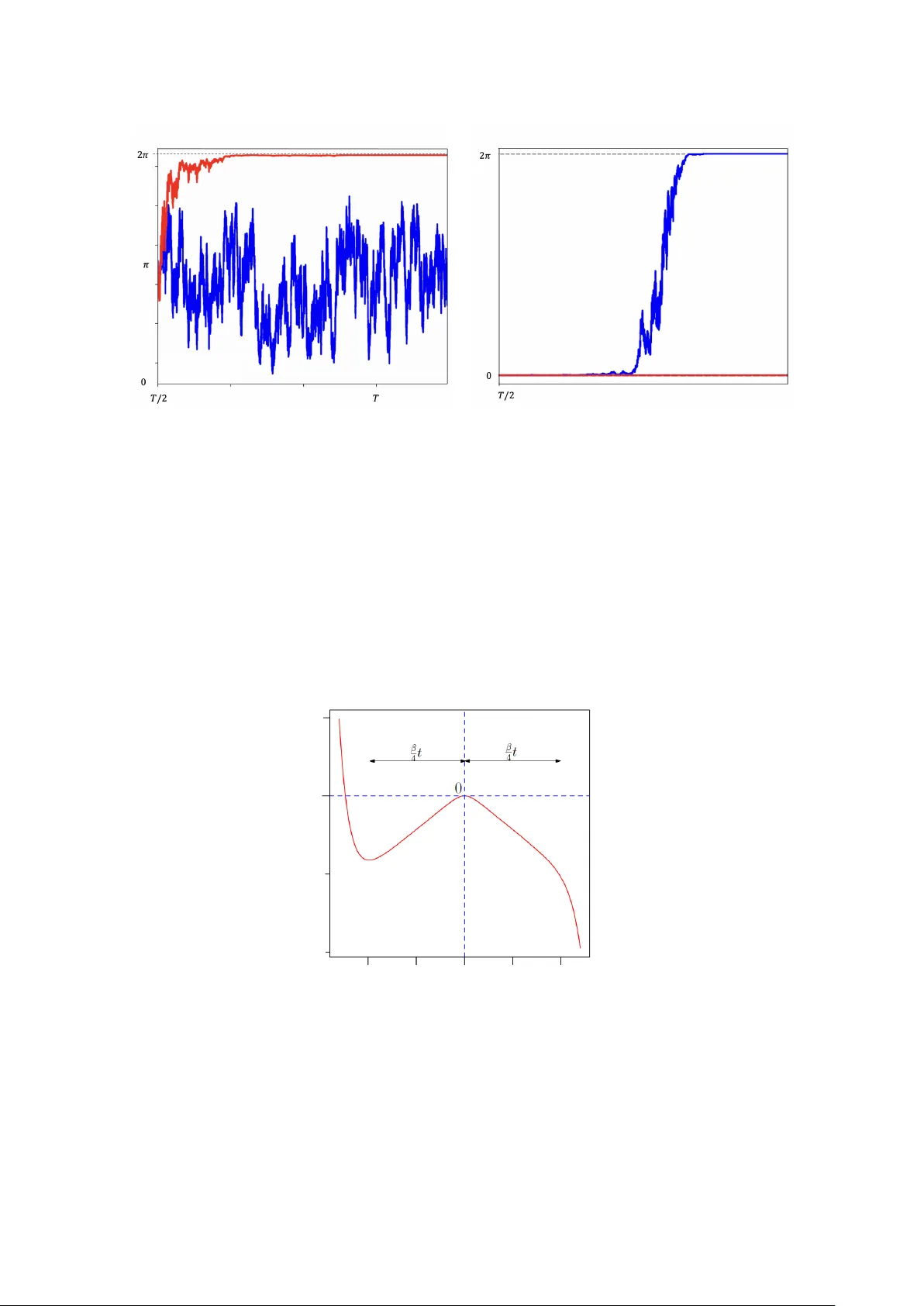
LONG-RANGE CORRELA TION OF THE SINE β POINT PR OCESS LA URE DUMAZ AND MAR TIN MAL VY Abstra ct. W e study the correlations of the celebrated Sine β p oin t process. This p oint pro cess arises as the bulk scaling limit of β -ensem bles and has a geometric description through the Bro wnian carousel, as shown by V alkó and Virág (2009). W e establish that the a veraged k -p oint truncated correlation functions decay p olyno- mially in the limit of large separation. W e show that the deca y exp onent is of order 1 /β for large β . This is a step tow ards a conjecture by F orrester and Haldane regarding the exact asymptotics of the t wo-point correlation function, a problem recently addressed by Qu and V alkó (2025). Our pro ofs, which rely on a careful analysis of the coupling of dif- fusions asso ciated with the Brownian carousel, hold for all β > 0 and k ≥ 1 , signiﬁcantly extending previous results limited to sp eciﬁc v alues of β or k . Contents 1. In tro duction 1 2. Strategy of pro of and pro of of the theorems 6 3. Beha vior after large times, Pro of of Lemma 2.3 16 4. Appro ximating diﬀusions with a discrete scheme 21 5. Asymptotic indep endence betw een t w o driving Bro wnian motions 22 6. Generalization to any n umber of in terv als 24 References 29 1. Intr oduction 1.1. Log-gases and random matrices. The Sine β p oin t pro cess is a fundamen tal ob ject arising in Random Matrix Theory (RMT) and statistical mec hanics. In RMT, it describ es the bulk scaling limit of the eigen v alue distributions of the celebrated inv ariant Gaussian ensem bles for β = 1 , 2 , 4 , as well as the general β > 0 tridiagonal ensem bles in tro duced b y Dumitriu and Edelman [5]. Their joint probabilit y distribution is giv en by the Gibbs measure 1 Z n,β Y 1 ≤ i 0 . Using the tridiagonal matrix mo dels of [5], they prov ed the con v ergence of the rescaled point pro cess in the bulk of the sp ectrum. Sp eciﬁcally , for an y energy lev el E ∈ ( − 2 , 2) , the recaled point pro cess n X k =1 δ n √ 4 − E 2 ( λ k / √ n − E ) con v erges v aguely as n → ∞ to wards a non-trivial, translation-inv arian t random point pro cess: the Sine β p oin t pro cess (see also [12] for an alternativ e construction using Circular β -ensembles). Moreo v er their approac h gives a geometrical in terpretation of the Sine β p oin t pro cess via the Brownian carousel. The coun ting function of the Sine β pro cess is describ ed b y λ 7→ α λ (+ ∞ ) / 2 π , where the phases ( α λ ) λ ∈ R are solutions to a family of coupled sto chastic diﬀeren tial equations driven b y a complex Bro wnian motion. This construction directly implies that Sine β is inv ariant under translations, with intensit y 1 / (2 π ) but it also gives access to ﬁne statistics, including large gap probabilities [26] and Cen tral Limit Theorems [13]. The V ariational Appr o ach: R enormalize d Ener gy. T o understand the microscopic b eha v- ior of log-gases, Serfat y and Leblé [15] developed a v ariational framework based on the “Renormalized Energy” of p oin t pro cesses P , denoted b y W ( P ) . They pro v ed that, up to extraction, the av eraged microscopic p oint pro cess con v erges to point pro cesses P that minimize the free energy functional: F β ( P ) = β W ( P ) + en t[ P | Π] , (1.2) where ent[ ·| Π] denotes the sp eciﬁc relativ e entrop y with respect to a P oisson p oint pro cess Π of intensit y 1 / (2 π ) . The Sine β p oin t pro cess is then identiﬁed as the unique minimizer of F β among translation- in v ariant pro cesses [6]. The Statistic al Physics Persp e ctive: DLR Equations. In [4], Dereudre, Hardy , Leblé and Maïda obtain an alternativ e description of Sine β as an inﬁnite Gibbs measure at inv erse temp erature β > 0 asso ciated with the logarithmic pair p oten tial interaction. More pre- cisely , they sho w that Sine β solv es the canonical Dobrushin-Lanford-Ruelle (DLR) equations for a sp eciﬁc renormalized logarithmic potential. While it is kno wn that Sine β solv es these DLR equations, the uniqueness of the solution remains an op en question for general β , except for the case β = 2 due to the determinantal structure. 1.2. Main results of the pap er. Consider a point pro cess such that E h (# p oints in B ) k i < ∞ . for all k and bounded Borel set B . Then, its k -p oint correlation measure ρ ( k ) is deﬁned suc h that for an y p airwise disjoint Borel sets B 1 , . . . , B k , one has: E h k Y i =1 (# p oints in B i ) i = ρ ( k ) ( B 1 × · · · × B k ) . (See paragraph 2.4 b elow for a more precise deﬁnition). W e will use the notation Sine β ( B ) for the num b er of points of a p oint pro cess with law Sine β in a given Borel set B . In particular, E [ Sine β ( B )] = ρ (1) ( B ) . LONG-RANGE CORRELA TION OF THE SINE β POINT PROCESS 3 A consequence of the DLR equations is that for all β > 0 , such correlation measures hav e a densit y with resp ect to Leb egue measure, called correlation functions, see [19] for more details. F or the Sine β p oin t process, with a slight abuse of notation, we simply denote b oth the measure and the densit y by ρ ( k ) in the rest of the article. The main ob jective of the presen t article is to prov e asymptotic b ounds on the correlation functions for the Sine β p oin t pro cess when the p oints are widely separated, and which hold for all parameters β > 0 . Two-p oint c orr elation function. Let us ﬁrst state our result for k = 2 as it is the most insigh tful case. F or any β > 0 , w e deﬁne the trunc ate d t w o-p oint correlation function as ρ (2) T ( x, y ) = ρ (2) ( x, y ) − ρ (1) ( x ) ρ (1) ( y ) . In our case, note that ρ (1) ( x ) = 1 / (2 π ) . Since Sine β is translation in v ariant, w e will sligh tly abuse notation in the follo wing b y writing ρ (2) T ( r ) for ρ (2) T ( x, x + r ) . W e analyze in this paper a lo cally a v eraged v ersion of the truncated correlation function and sho w its polynomial deca y . Theorem 1.1 (Deca y of the truncated t wo-point correlation function) . Ther e exist an absolute c onstant c > 0 and for al l β , λ 0 > 0 a c onstant C = C ( β , λ 0 ) > 0 so that for any λ ≤ λ 0 , r ≥ 1 ,    Z λ 0 ρ (2) T ( x + r )d x    ≤ C r − cβ 1+ β 2 . This result relates to a conjecture b y F orrester and Haldane in [7]. Using the Calogero- Sutherland Hamiltonian (see e.g. Chapter 5 of the b o ok of Sutherland [24]) and Haldane’s theory ab out compressible quantum ﬂuids [9], F orrester predicted the asymptotic behavior for the tw o-p oin ts truncated correlation function. He established this rigorously for even in tegers v alues of β (see Prop osition 13.2.4 in [7]) and derived analogous results for rational β under a truncation sc heme (see F orm ula 13.226 in [7]). Extracting the leading-order b eha vior, the asymptotics is predicted to be ρ (2) T ( r ) ∼                  − 1 π 2 β r 2 for β < 2 , − 1 2 π 2 r 2 + cos r 2 π 2 r 2 for β = 2 , a 1 cos r r 4 /β for β > 2 , (1.3) with an explicitly giv en co eﬃcient a 1 . Our Theorem 1.1 sp eciﬁes that the deca y rate decreases for large β as c/β . This b eha vior is not surprising as the Sine β p oin t pro cess crystallizes to w ards the “Pic k et F ence” conﬁguration U + 2 π Z (where U is uniform on [0 , 2 π ] ) as β → ∞ . Conv ersely , as β tends to 0 , Sine β con v erges to a Poisson p oin t process (see [1] and [6]), for whic h the truncated correlation functions v anish. Here from the F orrester/Haldane conjecture, one exp ects that the higher co eﬃcien t is equal to 2 but w e obtain only some exponent of order O ( β ) . Note that when β = 2 , the Sine β pro cess has a determinan tal structure and ρ ( k ) ( x 1 , · · · , x k ) = det ( K ( x i , x j )) 1 ≤ i,j ≤ k , K ( x, y ) : = sin(( x − y ) / 2) π | x − y | . In particular, the t w o-p oin ts truncated function ρ (2) T admits the explicit form ula ρ (2) T ( r ) = − sin 2 ( r / 2) π 2 r 2 . A Ber ezinskii–Kosterlitz–Thouless (BKT) phase transition is exp ected at β = 2 (see [17, Remark 41]) and this critical v alue is conjectured to be at the junction in betw een the 4 LAURE DUMAZ AND MAR TIN MAL VY univ ersal deca y | x − y | − 2 and oscillatory β -dep enden t deca y , as seen in the F orrester–Haldane conjecture (1.3). V ery recen tly , a stronger v ersion of Theorem 1.1 was obtained by Qu and V alkó in a preprin t [22] that app eared on ArXiv while w e w ere ﬁnishing the present pap er. They deriv ed the exact ﬁrst order asymptotics (equal to r − 4 /β ) for β ≥ 4 , and obtained non- optimal b ounds for small v alues of β , similar to our own. Ho w ev er, our metho dology diﬀers signiﬁcan tly from theirs. Their approach relies on an exact corresp ondence b etw een the t w o p oints function of Sine β and the one-p oint function of the Hua Pickrell process with parameters ( β , β / 2) (which describ es Sine β conditioned to ha v e a p oint at the origin). In con trast, our strategy inv olv es a probabilistic alternative to these algebraic identities. This will allow us to treat the higher k -p oint correlation functions for k ≥ 2 . Ev en more recently , Assiotis and Na jnudel [2] established an exact identit y of the k -p oint correlation function in terms of some momen ts of the Hua-Pickrell sto chastic zeta function (deﬁned b y Li and V alk ó in [18]) with parameters ( β , k β / 2) . While exact, extracting the large separation asymptotics from this identit y seems to remain highly non-trivial. Gener al k -p oint c orr elation function. Our main result generalizes Theorem 1.1 to arbitrary k -p oint correlation functions. Let us ﬁx k ≥ 2 and 1 ≤ k 0 < k . W e consider the p artial ly trunc ate d functions asso ciated with t w o given clusters ρ ( k ) ( x 1 , · · · , x k ) − ρ ( k 0 ) ( x 1 , · · · , x k 0 ) ρ ( k − k 0 ) ( x k 0 +1 , · · · , x k ) , for x 1 , · · · , x k ∈ R . Heuristically , this quantit y measures the “correlation” b etw een the ﬁrst cluster ( x 1 , · · · , x k 0 ) and the second cluster ( x k 0 +1 , · · · , x k ) . It would v anish for a Poisson p oin t pro cess. F or an y scalar r ∈ R and x = ( x 1 , · · · , x d ) ∈ R d , w e use the notation x + r for the translated v ector ( x 1 + r, · · · , x d + r ) . In the follo wing result, we k eep track of ho w the pre-factor to the deca y rate depends on the parameter k and the cluster size. Theorem 1.2 (Decay of partially truncated k -p oint correlations) . Ther e exist an absolute p ositive c onstant c > 0 and, for any β > 0 and λ 0 > 0 , a c onstant C = C ( β , λ 0 ) > 0 such that the fol lowing holds. Fix k ≥ 2 and 1 ≤ k 0 < k . L et I 1 ⊂ ( R − ) k 0 and I 2 ⊂ ( R + ) k − k 0 b e two pr o ducts of disjoint intervals wher e e ach interval has length at most λ 0 . L et L b e the diameter of the union of the intervals c omp osing I 1 and I 2 . Then, we have for al l r ≥ 1 ,    Z I 1 Z I 2  ρ ( k ) ( x , y + r ) − ρ ( k 0 ) ( x ) ρ ( k − k 0 ) ( y + r )  d x d y    ≤ K ( k , L ) r − c β 1+ β 2 , (1.4) wher e the pr e-factor K ( k , L ) dep ends on k , L and the c onstant C as fol lows: K ( k , L ) = min( C k 3 e C L , C k k k/ 2 ) . Remark 1.3. The clusters I 1 := Q k 0 i =1 I i and I 2 := Q k i = k 0 +1 I i are c hosen in R − (resp. R + ) so that the distance b et w een ∪ i ≤ k 0 I i comp osing I 1 and ∪ k i = k 0 +1 ( I i + r ) comp osing the shifted b y r v ersion of I 2 is at least r . Due to the translation in v ariance of the correlation functions, the same result holds for any shifted domains I 1 + t := Q k 0 i =1 ( I i + t ) and I 2 + t := Q k i = k 0 +1 ( I i + t ) with t ∈ R . The most common pair-clustering scenario corresp onds to sending a single particle far aw a y that is k − k 0 = 1 . Recalling that ρ (1) ≡ (2 π ) − 1 , the b ound (1.4) becomes      Z I 1 Z λ 0 ρ ( k ) ( x , y + r ) − ρ ( k − 1) ( x ) 2 π ! d x d y      ≤ K ( k , L ) r − c β 1+ β 2 . (1.5) Remark 1.4. Let us analyze the behavior of the pre-factor K ( k , L ) in diﬀerent regimes of k and L . On one hand, if k is b ounded, K ( k , L ) is uniformly b ounded in L . On the other hand, for k large, the situation go es as follo ws. LONG-RANGE CORRELA TION OF THE SINE β POINT PROCESS 5 (1) Smal l cluster size: L is ﬁxe d or L = O (ln k ) . In this case, our b ound grows p olyno- mially in k . Note that ﬁtting k disjoint in terv als in to a domain of size O (ln k ) implies that the a v erage in terv al length is O ( ln k k ) . This corresp onds to a rare “o v ercro wding” ev en t. (2) Interme diate cluster size: ln k ≪ L ≪ k ln k . In this regime, our bound gro ws exp onen tially with L . The case where L is of order k represen ts the typical scenario for the p oin t pro cess (where eac h p oint lies in an in terv al of size O (1) ). (3) A rbitr arily lar ge cluster size: L ≫ k ln k . Here, the b ound is dominated b y the second term, yielding a sub-factorial gro wth of k k/ 2 . It is instructive to compare this gro wth with that of the moments of the num ber of p oints inside the in terv als. By Hölder’s inequality , for an y disjoin t interv als I i of length b ounded by λ 0 , Z I 1 ×···× I k ρ ( k ) ( x )d x = E h k Y i =1 Sine β ( I i ) i ≤ E h ( Sine β ([0 , λ 0 ])) k i . As shown in Prop osition 2.2, the random v ariable Sine β ([0 , λ 0 ]) is sub-Gaussian, hence its moments satisfy E [( Sine β ([0 , λ 0 ]) k ] ≤ C k k k/ 2 . Since the uniform b ounds K ( k , ∞ ) satisfy the same gro wth rate, they can b e viewed as optimal in this sense. The previous results directly imply similar b ounds for the k -p oin t truncated correlation functions. These are deﬁned recursiv ely as follo ws: ρ (1) T ( x 1 ) = ρ (1) ( x 1 ) and ρ ( k ) T ( x 1 , · · · , x k ) = ρ ( k ) ( x 1 , · · · , x k ) − X π =( J 1 , ··· ,J j ) , π  = { 1 , ··· ,k } ρ ( | J 1 | ) T ( X J 1 ) · · · ρ ( | J j | ) T ( X J j ) , (1.6) where the sum runs ov er all the partitions π of { 1 , · · · , k } except the trivial one { 1 , · · · , k } , and X ( i 1 , ··· ,i j ) := ( x i 1 , · · · , x i j ) . In the context of p oint pro cesses, correlation functions act as the natural analogs of moments of a random v ariable, while truncated correlation functions corresp ond to their cum ulan ts. Indeed, the k -p oint truncated correlation function describ es only the k -b o dy correlations, b y factoring out the correlations from smaller subsets. F rom Theorem 1.2, one can obtain as w ell the decay of the k -p oint truncated correlation functions, up on c hanging the pre-factor K ( k , L ) : Theorem 1.5 (T runcated k -p oint correlation deca y) . Ther e exist an absolute p ositive c on- stant c > 0 and for any β > 0 and λ 0 > 0 , a c onstant C = C ( β , λ 0 ) > 0 such that the fol lowing holds. L et us ﬁx k ≥ 2 and take ( I i ) 1 ≤ i ≤ k p airwise disjoint intervals of size atmost λ 0 . W e have:    Z I 1 ×···× I k ρ ( k ) T ( x 1 , · · · , x k ) d x 1 · · · d x k    ≤ K 2 ( k )  max S 1 ⊔ S 2 = { 1 , ··· ,k } dist  ∪ i ∈ S 1 I i , ∪ i ∈ S 2 I i   − c β 1+ β 2 , wher e K 2 ( k ) = C k k ! k k/ 2 . This theorem is a direct consequence of Theorem 1.2. W e refer to Section 2.4 for a pro of. Let us brieﬂy discuss the implications of this last result. Informally , it establishes the asymptotic independence of regions which are spatially far. F or general p oint pro cesses, follo wing [14], the set of solutions to the DLR equations can be represen ted as conv ex com binations of extremal Gibbs states. Consequently , showing uniqueness is equiv alent to proving that there is a unique extremal state. F ollowing the framew ork established by Georgii [8], these extremal states are c haracterized by a trivial tail σ -algebra. When the in teractions are short-range, this prop ert y is equiv alen t to the deca y of partially truncated correlations. Dereudre et al. [4] prov ed that the Sine β pro cess satisﬁes the DLR equations, but uniqueness among translation-inv ariant solutions remains op en, except in the sp ecial case β = 2 . Our result on the decay of truncated correlations therefore strongly suggests 6 LAURE DUMAZ AND MAR TIN MAL VY that Sine β is an extremal state for the DLR equations, and that it should be their unique solution. This strongly relates to the uniqueness result of Erbar, Huesmann, and Leblé [6], who pro v ed that Sine β is the unique minimizer of the inﬁnite-v olume free energy among translation-in v ariant p oin t pro cesses. A c kno wledgmen ts. W e w ould lik e to thank Benedek V alkó and Y ah ui Qu for useful dis- cussions. Sp ecial thanks are due to Mathieu Lewin for his careful reading of a previous v ersion of this article and for his numerous helpful suggestions during its preparation. L.D. ac kno wledges the supp ort of ANR RANDOP ANR-24-CE40-3377 and LOCAL ANR-22- CE40-0012. 2. Stra tegy of pr oof and proof of the theorems 2.1. The sto chastic sine e quations . In [25], V alk ó and Virág giv e a description of the p oin t process Sine β in terms of a family ( α λ ) λ ∈ R of one-dimensional diﬀusion processes called the sto chastic sine e quations , whic h describ es the evolution of the h yp erb olic angle determined b y the Bro wnian carousel of parameter λ , its driving Brownian motion and its starting p oint, see Section 2.1 of [25]. In particular, the family ( α λ ) λ satisﬁes the sto chastic sine e quation : d α λ ( t ) = λ β 4 e − β 4 t d t + Re  ( e − iα λ ( t ) − 1)d W ( t )  , (2.1) with initial condition α λ (0) = 0 and where ( W ( t )) t ≥ 0 is a standard complex Brownian motion. In the latter, w e will denote f ( t ) := ( β / 4) e − β t/ 4 . Note that the family ( α λ ( s ) , s ≥ 0 , λ ∈ R ) has a unique solution deﬁned in [0 , + ∞ ) such that for all s ≥ 0 , λ 7→ α λ ( s ) is contin uous. An imp ortant property shared by the processes α λ for λ ∈ R is that, almost surely , they all conv erge to m ultiples of 2 π in the large time limit, see Figure 1 for a plot of a sim ulation of their tra jectories for t w o v alues of λ . By deﬁnition, almost surely , λ 7→ α λ (+ ∞ ) is righ t-con tinuous with left limits. It corresp onds to the coun ting measure of the Sine β p oin t pro cess:  Sine β  (0 , λ ]   λ ∈ R ( d ) =  α λ (+ ∞ ) 2 π  λ ∈ R . (2.2) Remark 2.1 ( β = 2 transition) . The BKT transition at β = 2 can b e hin ted in the change in the long-time behavior of the Brownian carousel according to the v alue of β : V alk ó and Virág prov e in [25] that the diﬀusion α λ con v erges from abov e a.s. if and only if β ≤ 2 . Let us recall imp ortant prop erties of the diﬀusion processes ( α λ ) λ ∈ R , already established in [25], that will b e useful in this pap er: (1) F or all λ, λ ′ ∈ R , α λ ′ − α λ has the same distribution as α λ ′ − λ ; (2) F or all t ≥ 0 , λ 7→ α λ ( t ) is increasing ; (3) F or all λ ≥ 0 , t 7→ ⌊ α λ ( t ) ⌋ 2 π is non-decreasing. Here, ⌊ x ⌋ 2 π = max(2 π Z ∩ ( −∞ , x ]) ; (4) F or all λ > 0 and all in tegers a, k , P ( Sine β [0 , λ ] ≥ a k ) ≤ 2  λ 2 π a  k . Prop ert y (1) ensures that the point pro cess Sine β is inv ariant under translation. This is easily obtained as the pro cess ˜ α : = α λ ′ − α λ is the solution of d ˜ α ( t ) = ( λ ′ − λ ) f ( t )d t + Re  ( e − i ˜ α ( t ) − 1)d ˜ W ( t )  , ˜ α (0) = 0 , with driving Brownian motion ˜ W ( t ) = R t 0 e − iα λ ( s ) d W ( s ) . Note that w e will use this repre- sen tation for the diﬀerence later on. LONG-RANGE CORRELA TION OF THE SINE β POINT PROCESS 7 Prop ert y (4) provides a control on the num ber of points in in terv als. In particular, it implies that the k factorial momen ts satisfy E  Sine β [0 , ε ] × · · · × ( Sine β [0 , ε ] − k + 1)  ≤ C k ε k , whic h implies the existence of the k -p oint correlation measures. In [10], Holcomb and V alk ó established precise tail estimates for o v ercro wding. The follo wing theorem extends their b ound to arbitrarily large interv als, pro viding a uniform estimate that we will use to obtain the pre-factor K ( k , L ) in Theorem 1.2. Theorem 2.2 (Overcro wding estimate, Holcomb, V alk ó, adapted from [10]) . F or al l β > 0 , ther e exists a c onstant C = C ( β ) such that for al l λ ≥ 1 and al l n ≥ C λ , P  Sine β [0 , λ ] ≥ n  ≤ exp  − ( β / 4) n 2 ln( n/λ )  . (2.3) Pr o of sketch. The authors sho w in [10] that there exists a p ositive constan t c = c ( β , λ 0 ) suc h that for all 0 < λ ≤ λ 0 and for n ≥ 1 , one has P  Sine β [0 , λ ] ≥ n  ≤ e − ( β / 2) n 2 ln( n/λ )+ cn ln( n +1) ln( n/λ )+ cn 2 . One has to trac k how the constan t c in their formula dep ends on λ 0 . Lo oking at their pro of of the upp er b ound, w e see that their argument remains v alid for arbitrarily large λ ≥ 1 and for n large enough with resp ect to λ , since the constan ts in v olved in their recursion dep end only on β . Moreov er, when n ≥ C ( β ) λ , the inequalit y cn ln( n + 1) ln( n/λ ) + cn 2 − ( β / 4) n 2 ln( n/λ ) ≤ 0 holds as long as the constant C ( β ) is c hosen large enough. This implies the result. □ Figure 1. (color online). T ra jectories of the diﬀusions α 6 (blue) and α 20 (red) for β = 1 . This realization of Sine 1 has tw o points in [0 , 6] and 4 points in [0 , 20] . Remark that the α λ can not go b elow a level 2 k π once it has b een crossed, and that the dynamics freeze after times m uc h larger than | log λ | . Let us no w rephrase Theorem 1.2 with the stochastic sine equations. Let us ﬁx the parameters β , λ 0 , k . Deﬁne J 1 := { 1 , · · · , k 0 } and J 2 := { k 0 + 1 , · · · , k } and the tw o pro ducts: I 1 := Y i ∈ J 1 I i , and I 2 := Y i ∈ J 2 I i , where I i := [ x i , x i + λ i ] . (2.4) Moreo v er, the interv al lengths satisfy λ i ≤ λ 0 . In the ﬁrst cluster 1 ≤ i ≤ k 0 , we choose x i so that the interv als I i are pairwise disjoin t and included in R − . In the second cluster k 0 + 1 ≤ i ≤ k , w e choose x i suc h that the in terv als are all disjoin t and included in R + . 8 LAURE DUMAZ AND MAR TIN MAL VY W e deﬁne α ( i ) ( t ) : = α x i + λ i ( t ) − α x i ( t ) , i ∈ J 1 , and α ( i ) ( t ) : = α r + x i + λ i ( t ) − α r + x i ( t ) i ∈ J 2 . By deﬁnition, we ha ve  Sine β ( I i 1 ) , i 1 ∈ J 1 , Sine β ( r + I i 2 ) , i 2 ∈ J 2  ( d ) =  α ( i ) (+ ∞ ) 2 π , i ∈ { 1 , · · · , k }  . (2.5) Correlations are encoded in the coupling b etw een the tw o families of diﬀusions i ∈ J 1 and i ∈ J 2 . As we will observe later, this coupling strongly depends on the diﬀusion α r d α r ( t ) = r f ( t )d t + Re  ( e − iα r ( t ) − 1) d W ( t )  , (2.6) and the complex Bro wnian motion W r ( t ) := Z t 0 e − iα r ( s ) d W ( s ) . The diﬀusions α ( i ) for i ∈ J 1 are given b y d α ( i ) ( t ) = λ i f ( t )d t + Re  ( e − iα ( i ) ( t ) − 1)d W ( i ) ( t )  , d W ( i ) ( t ) = e − iα x i ( t ) d W . Similarly , the diﬀusions α ( i ) for i ∈ J 2 are given b y d α ( i ) ( t ) = λ i f ( t )d t + Re  ( e − iα ( i ) ( t ) − 1)d W ( i ) ( t )  , d W ( i ) ( t ) = e − i ( α x i + r ( t ) − α r ( t )) d W r ( t ) . W e denote in the following W 1 : =  W (1) , · · · , W ( k 0 )  , W 2 : =  W ( k 0 +1) , · · · , W ( k )  . 2.2. Main steps of the proof of Theorems 1.1 and 1.2. In this section, we explain the main steps of the proof of Theorems 1.1 and 1.2. W e fully state the key lemmas, whose pro ofs are deferred to the subsequen t sections, and w e then provide the pro of of the Theorems. Deﬁne the time T r : = (4 /β ) ln r . This is the t ypical time at which our system of diﬀusions go es from an independent activ e dynamics to a dep endent frozen dynamics. Namely , • F or times smal ler than T r and for large v alues of the parameter r , the diﬀusion α r deﬁned in (2.6) has a strong drift and b ehav es almost deterministically . It follows the deterministic path given b y t 7→ r R t 0 f ( s ) ds = r (1 − e − β t/ 4 ) . As a consequence, the complex Bro wnian motion W is close to b eing indep endent of W r . W e obtain a go o d control of this phenomenon thanks to a discretization of the time interv al. • F or times gr e ater than T r , the diﬀusion α r b ecomes more unpredictable, which ef- fectiv ely creates correlations. Ho w ev er, its impact on the correlations is con trolled using that the diﬀusions ( α ( i ) , i = 1 , · · · , k ) hav e a slow dynamic after suc h time since their drift term is small. Figure 2 represents a plot of the real part of t 7→ e − iα r ( t ) and illustrates this transition. W e ﬁrst state a lemma showing that, after large times, the diﬀusion α λ is very close to its limiting v alue with high probabilit y . Lemma 2.3 (Finite time appro ximation) . F or al l β , λ 0 > 0 , ther e exists C = C ( β , λ 0 ) > 0 such that for al l λ ≤ λ 0 , for al l T ≥ 1 , we have P    α λ ( T ) − α λ (+ ∞ )   > π / 2  ≤ C exp  − (1 ∧ β ) T / 128  . LONG-RANGE CORRELA TION OF THE SINE β POINT PROCESS 9 Figure 2. Simulation of the oscillations of t 7→ cos( α r ( t )) , r = 100 , β = 4 . A t ﬁrst, the dynamic is deterministic. After times of order T r , randomness app ears, until the system gets frozen and conv erges to w ards 1 . This k ey lemma is one of the main tec hnical imput of the present paper. It relies on t w o facts: the ﬁrst one is that the regions around 2 π N + π are unstable equilibria for the diﬀusion α λ . Using Girsanov’s theorem, we are able to prov e that it escap es rapidly from these. Then, as long as the diﬀusion escap ed from neigh b orho o d of 2 π N + π , the multiples of 2 π are attractiv e. W e then turn to the time interv al where we exp ect that the t wo clusters b ehav e in an almost indep endent w a y . Let us ﬁrst state the lemmas for k = 2 , as they need some reﬁnemen t for general k -p oint correlation functions. T ake 1 x 1 := 0 and x 2 := 0 . W e simply ha v e t wo diﬀusions α (1) and α (2) driv en by W (1) = W and W (2) = W r . Fix n ≥ 1 and let ( t j := j T /n, j = 1 , · · · , n ) b e a discretization of the in terv al [0 , T ] . The follo wing lemma shows that, for large times T and large integer n , the diﬀusion α ( i ) and a discretized v ersion of it, measurable w.r.t. ( W ( i ) ( t j ) , j = 1 , · · · , n ) are close to each other with high probabilit y . Lemma 2.4 (Discretization) . L et β , λ 0 > 0 . Ther e exists C = C ( β , λ 0 ) > 0 such that for al l λ 1 , λ 2 ≤ λ 0 , for al l T > 0 , for al l inte ger n , and for i = 1 , 2 , ther e exists a pie c ewise-c onstant pr o c ess α ( i ) p . c . , me asur able with r esp e ct to the r andom ve ctors ( W ( i ) ( t j ) , j = 1 , · · · , n ) , such that P    α ( i ) p . c .  T  − α ( i )  T    ≥ π / 3  ≤ C e 4 T n . W e then con trol the total v ariation distance betw een the discretizations of ( W (1) , W (2) ) and of the independent coupling W (1) ⊗ W (2) . Lemma 2.5 (Upp er b ound for total v ariation) . L et β > 0 . Ther e exists C = C ( β ) > 0 such that for al l T , r > 0 and for al l n ∈ N , we have d T V   W (1) ( t j ) , W (2) ( t j )  n j =1 ,  W (1) ( t j ) ⊗ W (2) ( t j )  n j =1  ≤ C n 3 / 2 e β 4 T r . 1 Note that to b e in the exact setting of Theorem 1.2, we would need to tak e x 1 := − λ but it do es not c hange the b ounds. 10 LAURE DUMAZ AND MAR TIN MAL VY Note that the total v ariation distance is well-con trolled for times T smaller than T r , which is exp ected since correlations app ear after T r . When extending these results to general k -p oint correlation functions, we need the fol- lo wing reﬁnement of Lemmas 2.4 and 2.5. Lemma 2.6. L et β , λ 0 > 0 . Ther e exists a c onstant C = C ( β , λ 0 ) > 0 such that the fol lowing holds. L et k , n ≥ 1 b e inte gers, 1 ≤ k 0 < k and r e c al l that J 1 = { 1 , · · · , k 0 } and J 2 = { k 0 + 1 , · · · , k } . F or al l T , r > 0 and al l λ i ≤ λ 0 and x i chosen as in (2.4) , one c an c onstruct r andom variables ˜ W 1 ∈ C k 0 × n and ˜ W 2 ∈ C ( k − k 0 ) × n on the same pr ob ability sp ac e as the original diﬀusions ( α ( i ) ) 1 ≤ i ≤ k as wel l as pie c ewise c onstant pr o c esses ( α ( i ) p . c . ) 1 ≤ i ≤ k such that • F or i ∈ J 1 , ( α ( i ) p . c . ) i ∈ J 1 is me asur able w.r.t. ˜ W 1 and for i ∈ J 2 , ( α ( i ) p . c . ) i ∈ J 2 is me a- sur able w.r.t. ˜ W 2 ; • The total variation distanc e satisﬁes d T V   ˜ W 1 , ˜ W 2  ,  ˜ W 1 ⊗ ˜ W 2   ≤ C k 3 n 5 / 2 e β 4 T r ; • The discr etization err or is b ounde d by sup 1 ≤ i ≤ k P    α ( i ) p . c .  T  − α ( i )  T    > π / 2  ≤ C e 4 T n . Recall that the diﬀusions in the cluster J 1 are driven b y W 1 and in the cluster J 2 b y W 2 . The main technical issue for large k is that strong correlations within eac h cluster can cause the co v ariance matrices of the random v ectors ( W ( i ) ( t j ) , j = 1 , · · · , n, i ∈ J ℓ ) for ℓ = 1 or 2 to b ecome nearly singular. Because b ounds on the total v ariation distance typically dep end on the in v erse of these co v ariance matrices, suc h near-degeneracies cause standard decoupling b ounds to blo w up, counterbalancing the p olynomial decay induced b y the os- cillations of α r . T o preven t this, w e use another approximation of the contin uous processes W 1 and W 2 using a sp ectral regularization tec hnique. This regularization ensures that the total v ariation distance remains con trolled while still providing a precise discretization of the diﬀusions. 2.3. Pro of of Theorems 1.1 and 1.2. W e fo cus on the proof of Theorem 1.2. Indeed, applying it with k = 2 taking the interv als [0 , 1] and [ r , r + λ ] and using translation in v ariance w e immediately obtain the result of Theorem 1.1. Recall that I 1 := Q k 0 i =1 I i and I 2 := Q k i = k 0 +1 I i and that J 1 = { 1 , · · · , k 0 } and J 2 = { k 0 + 1 , · · · , k } , and in tro duce the products P 1 := k 0 Y i =1 Sine β ( I i ) , P 2 := k Y i = k 0 +1 Sine β ( r + I i ) . W e need to b ound from abov e    E  P 1 × P 2  − E  P 1  E  P 2     . The ﬁrst step is to introduce a cutoﬀ on the pro ducts in the exp ectations and decomp ose it in to probabilities as    E  ( P 1 × P 2 ) 1 {P 1 ≤ m, P 2 ≤ m }  − E  P 1 1 {P 1 ≤ m }  E  P 2 1 {P 2 ≤ m }     , ≤ m 4 sup p 1 ≤ m, p 2 ≤ m    P  P 1 = p 1 , P 2 = p 2  − P  P 1 = p 1  P  P 2 = p 2     . (2.7) Recall that we hav e Sine β ( I i ) := α ( i ) (+ ∞ ) / 2 π for i ∈ J 1 , and Sine β ( I i + r ) := α ( i ) (+ ∞ ) / 2 π for i ∈ J 2 . LONG-RANGE CORRELA TION OF THE SINE β POINT PROCESS 11 In the pro ducts P 1 and P 2 , up to a small error that we con trol, one can replace the v alues α ( i ) (+ ∞ ) by their appro ximations α ( i ) p.c. ( T ) . More precisely , if ⌊ x ⌉ denotes the smallest closest integer of x , w e use ⌊ α ( i ) p.c. ( T ) / (2 π ) ⌉ . As so on as | α ( i ) p.c. ( T ) − α ( i ) (+ ∞ ) | < π , the t w o v alues coincide since α ( i ) (+ ∞ ) / (2 π ) is an in teger. Let us denote the new pro ducts for q = 1 , 2 ˆ P q := Y i ∈ J q  α ( i ) p.c. ( T )  . F or any even ts A , Z , X , Y , w e ha v e the inequalities   P [ Z ] − P [ X ] P [ Y ]   ≤   P [ Z, A ] − P [ X , A ] P [ Y , A ]   + 2 P [ A c ] , and   P [ Z, A ] − P [ X , A ] P [ Y , A ]   ≤   P [ Z ] − P [ X ] P [ Y ]   + 2 P [ A c ] . Applied to the probabilities in (2.7), it giv es    P  P 1 = p 1 , P 2 = p 2  − P  P 1 = p 1  P  P 2 = p 2     ≤    P  ˆ P 1 = p 1 , ˆ P 2 = p 2  − P  ˆ P 1 = p 1  P  ˆ P 2 = p 2     + 4 P  ∪ k i =1 {| α ( i ) p.c. ( T ) − α ( i ) ( ∞ ) | ≥ π }  . W e b ound the ﬁrst term b y the total v ariation distance betw een the n × k dimensional complex vectors ( ˜ W 1 , ˜ W 2 ) and ( ˜ W 1 ⊗ ˜ W 2 ) of Lemma 2.6    P  ˆ P 1 = p 1 , ˆ P 2 = p 2  − P  ˆ P 1 = p 1  P  ˆ P 2 = p 2     ≤ d T V   ˜ W 1 , ˜ W 2  ,  ˜ W 1 ⊗ ˜ W 2   . W e use a union b ound on the second term and split each error term in to tw o parts P h   α ( i ) p.c. ( T ) − α ( i ) ( ∞ )   ≥ π i ≤ P h   α ( i ) p.c. ( T ) − α ( i ) ( T )   ≥ π 2 i + P h   α ( i ) ( T ) − α ( i ) ( ∞ )   ≥ π 2 i , whic h are con trolled thanks to Lemma 2.6 and Lemma 2.3. By c ho osing the parameters as T = 4 41+ β log r and n = e (16 − β ) T / 14 r 2 / 7 (a slightly suboptimal, y et asymptotically tight c hoice), we obtain the b ound    E h ( P 1 × P 2 )1 {P 1 ≤ m, P 2 ≤ m } i − E h P 1 1 {P 1 ≤ m } i E h P 2 1 {P 1 ≤ m } i    ≤ C m 4 k 3 r − c β , (2.8) for c β = 1 ∧ β 32(41+ β ) and some C := C ( β , λ 0 ) . In the following, w e will use again C for some constan t dep ending only on β and λ 0 that may c hange from line to line. It remains to bound: E h ( P 1 × P 2 ) 1 {P 1 ≥ m } i , E h P 1 1 {P 1 ≥ m } i E  P 2  , and the symmetric terms obtained when exc hanging the index 1 and 2 . W e hav e t w o options to b ound these exp ectations and we use b oth of them to deal with the ﬁrst term, as the same calculations are v alid for the other terms. In the ﬁrst appr o ach, w e use the fact that the in terv als comp osing I 1 and I 2 are non- o v erlapping, and therefore, we hav e a go o d control on the total num ber of points in the union ov er all interv als in terms of the diameter of this union: P 1 ≤ exp  k 0 X i =1 Sine β ( I i ) − k 0  ≤ exp  Sine β  [ − L, 0]   . 12 LAURE DUMAZ AND MAR TIN MAL VY It gives P  P 1 ≥ m  ≤ P h Sine β  [ − L, 0]  ≥ ln m i ≤ C exp  − ( β / 4)  ln m  2 ln  ln m L  , ≤ C exp  − ( β / 4)(ln m ) 2  , v alid when m ≥ exp( C L ) for C := C ( β , λ ) , c hosen greater than e , using the o v ercro wding estimate of Theorem 2.2. Moreo v er, E  ( P 1 ) 4  ≤ E  1 {P 1 ≤ e C ( L +1) } ( P 1 ) 4  + ∞ X p = ⌊ e C ( L +1) ⌋ P  P 1 ≥ p 1 / 4  ≤ e 4 C ( L +1) + ∞ X p = ⌊ e C ( L +1) ⌋ C exp  − β 64  ln p  2  . By increasing C if necessary , one ma y supp ose that each in teger p in the series satisﬁes β ln p/ 64 ≥ 2 , which implies: C exp( C L ) + C ∞ X p = ⌊ e C L ⌋ p − 2 ≤ C exp( C L ) . In the same w a y , E  ( P 2 ) 4  ≤ C exp( C L ) . In total we obtain thanks to Hölder inequalit y: E h ( P 1 × P 2 )1 {P 1 ≥ m } i ≤ E  ( P 1 ) 4  1 / 4 × E  ( P 2 ) 4  1 / 4 × P  P 1 ≥ m  1 / 2 ≤ C exp( C L ) exp  − ( β / 8)(ln m ) 2  . (2.9) W e take ln m = c β ln r / 8 + C ( L + 1) . Up to increasing C , we may supp ose C β ≥ 16 , so that β (ln m ) 2 / 8 ≥ c β log r . The last term (2.9) is smaller than C exp( C L ) r − c β . Replacing m with its v alue in (2.8) yields the b ound with the pre-factor K 1 ( L, k ) := C e C L k 3 m ultiplied by 1 /r at a p ow er slightly smaller c β , say c β / 2 . In the se c ond appr o ach, w e use Hölder’s inequalit y to write E  ( P 1 ) 2  ≤ E h Sine β  [0 , λ 0 ]  2 k 0 i ≤ C 2 k 0 (2 k 0 ) k 0 . Therefore, using E  ( P 1 ) 2 1 {P 1 ≥ m }  ≤ E  ( P 1 ) 2  /m 2 and the fact that k k 0 0 ( k − k 0 ) k − k 0 ≤ k k , w e obtain E  ( P 1 × P 2 ) 1 {P 1 ≥ m }  ≤ C k k k/ 2 m . Cho osing m = r c β / 5 , we obtain the result with K ( ∞ , k ) and r − c β / 5 . Remark 2.7 (On the absolute p ow er constan t) . R emark that the c onstant c of The or em 1.2 c an b e taken e qual to 2 − 13 . If one want to ﬁnd the optimal value when β is lar ge, we c an get 1 / 32 with the ﬁrst appr o ach. LONG-RANGE CORRELA TION OF THE SINE β POINT PROCESS 13 2.4. Correlation functions of p oin t pro cesses and pro of of Theorem 1.5. Let us recall some basic facts ab out real-v alued p oin t processes that one can ﬁnd for example in Lenard [16]. A p oint c onﬁgur ation γ is a integer-v alued Radon measure (whic h can be iden tiﬁed with a lo cally ﬁnite m ultiset of p oints in R ). W e denote b y Conf ( R ) the space of p oin t conﬁgurations. A p oin t conﬁguration γ is said to b e simple if γ ( { x } ) ≤ 1 for an y x ∈ R . The space Conf ( R ) is Polish when equipp ed with the top ology of vague c onver genc e (see e.g. [11, Section 15.7]). A sequence ( γ n ) n ≥ 1 con v erges v aguely to γ if and only if for all con tin uous compactly supported functions f : R → R , X u ∈ γ n f ( u ) − → n →∞ X u ∈ γ f ( u ) . W e endow Conf ( R ) with its Borel σ -algebra. A simple p oin t pro cess Γ is by deﬁnition a random v ariable taking v alues in Conf ( R ) suc h that Γ is simple almost surely . The law of Γ is uniquely determined b y the collection of Laplace functionals E h exp  − X u ∈ Γ f ( u ) i ev aluated on all non-negativ e contin uous compactly supp orted functions f . The joint intensity me asur es (also called factorial momen t measures) of a simple p oint pro cess Γ , when they exist, are measures ρ ( k ) on R k deﬁned for any Borel set B ⊂ R k b y ρ ( k ) ( B ) = E h X ( x 1 ,...,x k ) ∈ Γ ∧ k 1 B ( x 1 , . . . , x k ) i , where Γ ∧ k := { ( x 1 , . . . , x k ) ∈ Γ k , x i  = x j } denotes the set of k -tuples of distinct p oints of Γ . When B = D 1 × · · · × D k with D 1 , . . . , D k b eing m utually disjoint Borel subsets of R , this simpliﬁes to ρ ( k ) ( D 1 × · · · × D k ) = E h k Y i =1 Γ( D i ) i , where Γ( D i ) denotes the n um b er of p oin ts of Γ in D i . When one allo ws for ov erlaps betw een the sets D j , the situation is more delicate. F or example, taking B = D k yields the k -th factorial moment ρ ( k ) ( D k ) = E h Γ( D )! (Γ( D ) − k )! i . If Γ( D ) has exp onen tial tails for all b ounded Borel sets D , then the measures ρ ( k ) exist for all k . Moreov er, under this condition, the family ( ρ ( k ) ) k ≥ 1 uniquely determines the law of Γ : the moments m p : = E [Γ( D ) p ] characterize uniquely the la w of Γ( D ) as they grow slow er than ( C p ) p , therefore satisfy Carleman’s condition X p ≥ 1 ( m 2 p ) 1 / (2 p ) = + ∞ . If the measures ρ ( k ) are absolutely con tin uous with respect to the Leb esgue measure on R k , w e sa y that the point pro cess admits c orr elation functions (or joint intensities). With an abuse of notation, w e denote their densities again by ρ ( k ) ( x 1 , · · · , x k ) . The function ρ (1) is called the density of states (or simply intensit y). When the p oint pro- cess is translation-inv arian t, ρ (1) is constant. More generally , translation-inv ariance implies that ρ ( k ) ( x 1 + r , . . . , x k + r ) = ρ ( k ) ( x 1 , . . . , x k ) for all r ∈ R . 14 LAURE DUMAZ AND MAR TIN MAL VY Correlation functions are crucial for computing sev eral in teresting observ ables. F or in- stance, the discrepancy of a b ounded Borel set B is giv en by: Disc ( B ) : = V ar (Γ( B )) = Z B × B  ρ (2) ( x, y ) − ρ (1) ( x ) ρ (1) ( y )  d x d y + Z B ρ (1) ( x )d x. The existence of correlation functions (as densities, opposed to measures) is a non-trivial result. F or the Sine β p oin t pro cess, the existence of the measures ρ ( k ) is guaranteed by the exp onen tial tails of Sine β ( B ) for any b ounded Borel set B (see Poin t 4 in Subsection 2.1). F urthermore, one can pro v e that they admit densities for example using the DLR equations obtained in [4], w e refer to [19] for more details. W e hav e deﬁned in this pap er tw o quan tities to control the b ehavior of correlation func- tions when some p oin ts are widely separated. The ﬁrst is the (t w o clusters) p artial ly trun- c ate d c orr elation function : ρ ( k ) ( x 1 , · · · , x k ) − ρ ( k 0 ) ( x 1 , · · · , x k 0 ) ρ ( k − k 0 ) ( x k 0 +1 , · · · , x k ) . The second is the k -p oint trunc ate d c orr elation functions . As men tioned ab ov e, they are deﬁned recursively as follo ws: ρ (1) T ( x 1 ) = ρ (1) ( x 1 ) and ρ ( k ) T ( x 1 , · · · , x k ) = ρ ( k ) ( x 1 , · · · , x k ) − X π =( J 1 , ··· ,J j ) , π  = { 1 , ··· ,k } ρ ( | J 1 | ) T ( X J 1 ) · · · ρ ( | J j | ) T ( X J j ) , where the sum runs o v er all the partitions π = { J 1 , · · · , J j } of { 1 , · · · , k } except the trivial one { 1 , · · · , k } and X J := ( x i ) i ∈ J . Using the Möbius inv ersion form ula on the partially ordered set of partitions of { 1 , · · · , k } , one can express ρ ( k ) T in terms of the ρ ( i ) ’s as ρ ( k ) T ( x 1 , · · · , x k ) = k X j =1 ( − 1) j − 1 ( j − 1)! X π =( J 1 , ··· ,J j ) ρ ( | J 1 | ) ( X J 1 ) · · · ρ ( | J j | ) ( X J j ) , (2.10) where the second sum runs ov er all partitions π with exactly j blocks. Suc h com binatorial iden tities are closely related to the Stirling n um b ers of the second kind  k j  , whic h coun ts the num ber of partitions of a k -element set into j non-empty blo cks, and the ordered Bell n umbers Bell ( k ) which coun t the num b er of ordered partitions of a k -element set. They are deﬁned as Bell ( k ) = k X j =0  k j  j ! . As k → + ∞ , the ordered Bell num bers admit the asymptotic Bell ( k ) ∼ k ! 2(ln 2) k +1 , see e.g. [27] for a detailed o v erview ov er cumulan ts and com binatorics on partitions. A uniform b ound on the partially truncated correlation functions yields con trol o v er fully truncated correlation functions, up to a go o d control on the in tegrated correlation functions and the b ound X π =( J 1 , ··· ,J j ) ( j − 1)! = k X j =0  k j  ( j − 1)! ≤ Bell ( k ) , (2.11) where the sum runs ov er all the partitions of { 1 , · · · , k } (including the trivial partition equal to { 1 , · · · , k } ). One can sho w that the sum on the left hand side is equal to 2 Bell ( k − 1) . W e provide in the rest of the section a pro of of the decay of truncated correlation functions. More precisely , w e show that Theorem 1.5 is a consequence of Theorem 1.2. LONG-RANGE CORRELA TION OF THE SINE β POINT PROCESS 15 Pr o of. Consider the interv als I i , i = 1 , · · · , k . Let S 1 ⊔ S 2 = { 1 , · · · , k } b e a partition of the indices such that the distance b et ween the clusters A := ∪ i ∈ S 1 I i and B = ∪ i ∈ S 2 I i is maximized. Recall that w e hav e a sup er-m ultiplicative bound on the (in tegrated) k -p oint correlation function of the form Z Q k j =1 I j ρ ( k ) ( x )d x ≤ G k , G k := C k k k/ 2 , satisfying G k G k ′ ≤ G k + k ′ . Up to c hanging the constan t C = C ( β , λ 0 ) > 0 , w e hav e the rough a priori b ound u k := Z Q k i =1 I i | ρ ( k ) T ( x ) | d x ≤ k ! G k . (2.12) Indeed, using (2.10) and (2.11), w e ha v e u k ≤ X π =( J 1 , ··· ,J j ) ( j − 1)! j Y l =1  Z J l ρ ( | J l | ) ( x J l )d x J l  ≤ Bell ( k ) G k ∼ k ! (ln 2) k G k . Let us denote b y E k := Z x 1 ∈ Q i ∈ S 1 I i Z x 2 ∈ Q i ∈ S 2 I i   ρ ( k ) ( x 1 , x 2 ) − ρ ( k 0 ) ( x 1 ) ρ k − k 0 ( x 2 )   d x the decoupling of clusters asso ciated to S 1 and S 2 , and th us to A and B . W e write the diﬀerence as ρ ( k ) ( x 1 , x 2 ) − ρ ( k 0 ) ( x 1 ) ρ ( k − k 0 ) ( x 2 ) = X π ∈ Π( A,B ) Y S ∈ π ρ ( | S | ) T ( x S ) , where Π( A, B ) denotes the set of partitions π connecting A and B that is, partitions con- taining at least one blo ck S such that the v ector x S : = ( x i ) i ∈ S has co ordinates in b oth A and B . Isolating the trivial partition { 1 , · · · , k } , we obtain ρ ( k ) T ( x ) = ρ ( k ) ( x 1 , x 2 ) − ρ ( k 0 ) ( x 1 ) ρ ( k − k 0 ) ( x 2 ) − X π ∈ Π( A,B ) , π  = { 1 , ··· ,k } Y S ∈ π ρ ( | S | ) T ( x S ) . F or each π ∈ Π( A, B ) , π  = { 1 , · · · , k } , we iden tify a blo c k S ( A, B ) ∈ π connecting A and B which is of length s ∈ { 2 , · · · , k − 1 } . W e will ﬁrst sum on all the v alid blo cks S ( A, B ) of length s connecting A and B . W e hav e S ( k 0 , k − k 0 , s ) :=  k s  −  k 0 s  −  k − k 0 s  p ossible c hoices for this set. Then for an y ﬁxed S ( A, B ) , w e b ound the remaining pro duct o v er the other (integrated) terms of the partition Q S ∈ ( π \ S ( A,B )) ρ ( | S | ) T ( x S ) , using (2.12). This gives u k ≤ E k + k − 1 X s =2 S ( k 0 , k − k 0 , s ) u s G k − s . (2.13) Thanks to Theorem 1.2, w e hav e the upp er bound E k ≤ C k k k/ 2 d ( A, B ) − c β 1+ β 2 . One can chec k by induction that together with (3.1), w e obtain u k ≤ C k k ! k k/ 2 d ( A, B ) − c β 1+ β 2 , 16 LAURE DUMAZ AND MAR TIN MAL VY for a diﬀerent C (dep ending on λ 0 and β ) whic h giv es our result. Indeed, if w e supp ose that the inequality holds for all s < k , then u k ≤  C k k k/ 2 + k − 1 X s =2 C k  k s  s ! s s/ 2 ( k − s ) ( k − s ) / 2  d ( A, B ) − c β 1+ β 2 ≤ C k  k k/ 2 + k ! k − 1 X s =2 s s/ 2 ( k − s ) ( k − s ) / 2  d ( A, B ) − c β 1+ β 2 . The maximum of s s/ 2 ( k − s ) ( k − s ) / 2 is at one of the b oundaries s = 2 or s = k − 1 , for which w e get respectively 2( k − 2) ( k − 2) / 2 or ( k − 1) ( k − 1) / 2 . W e obtain the desired b ound. □ Remark 2.8. Note that we use d the b ound K ( k , ∞ ) for the pr o of inste ad of the optimal one. Inde e d, the sum over al l p artitions against the sup er-multiplic ative b ound G k − s dominates the asymptotics, le ading to k ! G k b ehavior in any c ase. 3. Beha vior after lar ge times, Pr oof of Lemma 2.3 3.1. Strategy of pro of. The goal of this section is to prov e Lemma 2.3 which states that for large time T , the diﬀusion α λ is close to its limiting v alue with high probability . F or a ﬁxed λ , the diﬀusion α λ satisﬁes the following Sto chastic Diﬀerential Equation (SDE) dα λ ( t ) = λf ( t ) dt + 2 sin( α λ ( t ) / 2) dB ( t ) , where B is a real standard Bro wnian motion. Supp ose that for some large time T , the p oint α λ ( T ) is at some distance from its limiting v alue. W e break this ev en t into t w o p ossibilities about the time interv al [ T / 2 , T ] : • Either the diﬀusion α λ did not get very close to any multiple of 2 π during the time in terv al [ T / 2 , T ] ; • Or the diﬀusion α λ reac hed a v alue v ery close to some m ultiple of 2 π during the in terv al [ T / 2 , T ] . In this case, it has to mov e aw a y from this m ultiple afterw ards. Indeed either the m ultiple corresp onds to α λ (+ ∞ ) and it has to b e at some distance of this p oint at time T , or it does not correspond to α λ (+ ∞ ) and α λ then has to reac h another m ultiple of 2 π . W e will pro v e that b oth ev en ts hav e small probability . On these tw o ev ents, one can hint the b eha vior of the diﬀusion α λ using an appropriate Girsano v’s c hange of measure, see (3.5). In Figure 3, we sampled in blue the tra jectories of α λ under this c hange of measure, as compared to their initial tra jectories in red. T o analyze the b ehavior of α λ , it is con v enien t to introduce the pro cess R := ln(tan( { α λ } 2 π / 4)) where { x } 2 π = x − (2 π ) ⌊ x/ (2 π ) ⌋ denotes the fractional part of x mo dulo 2 π . It ev olves according to the follo wing SDE: d R ( t ) = λ 2 f ( t ) cosh R ( t )d t + 1 2 tanh R ( t )d t + d B ( t ) . (3.1) The process R starts at −∞ at time 0 and ma y explo de to + ∞ at some ﬁnite time (it does so each time α λ reac hes a m ultiple of 2 π ). Once this happ ens, it immediately restarts at −∞ , which ensures that R is w ell deﬁned for all time t ≥ 0 . The adv an tage of studying R instead of α λ is that it is a diﬀusion with a constan t noise, evolving in a (non-stationary) p otential. This p otential has a well lo cated around − β t/ 4 at time t (which corresp onds to the v alues (2 π N ) + for α λ for large times) and an unstable equilibrium around 0 (corresp onding to π for the diﬀusion { α λ } 2 π ). Moreov er, on the segmen t well included in ( − β t/ 4 , 0) (resp. (0 , β t/ 4) ), the drift is almost constant equal to − 1 / 2 (resp. +1 / 2 ). This LONG-RANGE CORRELA TION OF THE SINE β POINT PROCESS 17 Figure 3. (color online). On the left ﬁgure, the blue path is a sample of the tra jectory of α λ started at π under the Girsanov change of measure (3.5) with parameters λ = 1 , β = 200 . On the right ﬁgure, the blue path is a sample of the tra jectory of α λ , started in 0 at time T / 2 “conditioned to attain 2 π ” (that is with the Girsanov change of measure of (3.5) un til it reaches π and then back to the initial measure), with λ = 1 , β = 4 . In both ﬁgures, the red path is a sample of the tra jectory of α λ without an y change of measure and with the same parameters and driving Bro wnian motion. explains why the diﬀusion ma y conv erge to a multiple of 2 π from b elow for β > 2 , whic h corresp onds to a tra jectory of R going growing to + ∞ thanks to its +1 / 2 drift without reac hing the slop e in (0 , β t/ 4) (whic h would lead to an explosion in ﬁnite time). See Figure 4 for a plot of the p oten tial at some large time t . Figure 4. Plot of the p oten tial of the diﬀusion R at a large time t , for λ = 1 . Let r 0 := (1 ∧ β ) T / 64 and deﬁne the following stopping time for R σ := inf { s ≥ T / 2 , | R ( s ) | ≥ r 0 } , τ := inf { s ≥ σ, | R ( s ) | ≤ r 0 / 2 } . W e will fo cus on the pro of in the case λ ≤ 1 . F or the more general case 1 ≤ λ ≤ λ 0 , it is suﬃcien t to w ait an extra time log λ to return to the case λ ≤ 1 . 18 LAURE DUMAZ AND MAR TIN MAL VY W e state in the follo wing lemma that it is unlik ely for R to stay a w a y from ±∞ during a long time in terv al [ T / 2 , T ] : Lemma 3.1 (Repulsion of the region near 0 ) . F or al l β , λ 0 > 0 , ther e exists C = C ( β , λ 0 ) such that for al l λ ≤ λ 0 , T ≥ 1 , P  σ ≥ T  ≤ C exp  − (1 ∧ β ) T / 128  . The pro of of Lemma 3.1 can b e found in Subsection 3.3. Then we state that when R reac hes some v alue near ±∞ , it is diﬃcult to lea v e it. Lemma 3.2 (Attraction to the region near ±∞ ) . F or al l β , λ 0 > 0 , ther e exists C = C ( β , λ 0 ) > 0 such that for al l λ ≤ λ 0 , T ≥ 1 , P  σ ≤ T , τ < + ∞  ≤ C exp  − (1 ∧ β ) T / 128  . The pro of of Lemma 3.2 can b e found in Subsection 3.2. Using the same pro of, we can obtain b etter estimates for large β , namely exp( − cβ T ) . the constant p olynomial decay for large β in Theorem 1.2 comes from Lemma 3.1. Using that when r ≫ 1 , 4 arctan( e r ) = 2 π − 4 e − r + O ( e − 3 r ) and 4 arctan( e − r ) = 4 e − r + O ( e − 3 r ) , Lemma 3.1 and Lemma 3.2 ab out R easily translate to α λ . Noting that 4 e − r 0 / 2 is smaller than π / 2 for large times T , Lemma 2.3 is corollary of these lemmas. In the following, we will denote by P x,t the probability measure asso ciated with the process satisfying R ( t ) = x . Note that we ha v e P = P −∞ , 0 . 3.2. A ttraction to the region near ±∞ : pro of of Lemma 3.2. On the probability P x,t , w e deﬁne σ to b e the ﬁrst hitting time of ± r 0 of the diﬀusion R after time t , and τ the ﬁrst hitting time of ± r 0 / 2 after σ . Let us introduce the ﬁrst explosion time τ ∞ of R after time σ . W e also deﬁne the stopping times σ + (resp. σ − ) as the ﬁrst hitting time of R of r 0 (resp. − r 0 ) after time t . W e aim to b ound P  σ ≤ T , τ < ∞  from ab ov e. Using the monotonicity prop erties of the diﬀusion R , it is suﬃcien t to b ound sup r ≥ r 0 sup t ∈ [ T / 2 ,T ] P r,t  τ < ∞ , τ ∞ > τ  (3.2) and P − r 0 ,T / 2  τ < ∞  . (3.3) T o justify this fact, w e divide the even t { σ ≤ T , τ < ∞} according to the p osition of the diﬀusion R at time T / 2 . • Case R ( T / 2) ≤ − r 0 : Here, σ = T / 2 . By monotonicit y , we obtain P  R ( T / 2) ≤ − r 0 , σ ≤ T , τ < ∞  ≤ P − r 0 ,T / 2  τ < ∞  . • Case R ( T / 2) ≥ r 0 : Similarly , σ = T / 2 and P  R ( T / 2) ≥ r 0 , σ ≤ T , τ < ∞  ≤ sup r ≥ r 0 P r,T / 2  τ < ∞  ≤ sup r ≥ r 0 P r,T / 2  τ < ∞ , τ ∞ < τ  + P r,T / 2  τ < ∞ , τ ∞ > τ  ≤ P − r 0 ,T / 2  τ < ∞  + sup r ≥ r 0 P r,T / 2  τ < ∞ , τ ∞ > τ  . • Case − r 0 < R ( T / 2) < r 0 : If R hits − r 0 b efore r 0 , we ha v e P  | R ( T / 2) | < r 0 , σ − = σ ≤ T , τ < ∞  ≤ P − r 0 ,T / 2 ( τ < ∞ ) . LONG-RANGE CORRELA TION OF THE SINE β POINT PROCESS 19 Con v ersely , if R hits r 0 b efore − r 0 , we ha v e P  | R ( T / 2) | < r 0 , σ + = σ ≤ T , τ < ∞  ≤ sup t ∈ [ T / 2 ,T ] P r 0 ,t ( τ < ∞ ) ≤ sup t ∈ [ T / 2 ,T ] P r 0 ,t  τ < ∞ , τ ∞ < τ  + P r 0 ,t  τ < ∞ , τ ∞ > τ  . Let us b ound (3.2) ﬁrst. F or r ≥ r 0 and t ∈ [ T / 2 , T ] , on the ev en t { τ < ∞ , τ ∞ > τ } , the diﬀusion remains in [ r 0 / 2 , + ∞ ) where the drift is b ounded b elow by 1 / 2 − e − r 0 / 2 . Hence, this probabilit y can b e b ounded by the probabilit y that a Brownian motion with constan t drift h 1 = 1 / 2 − e − r 0 / 2 starts at r 0 and hits r 0 / 2 in a ﬁnite time which is equal to exp( − h 1 r 0 ) . Since r 7→ r e − r/ 2 remains b ounded, w e get the upp er bound C e − r 0 / 2 . Let us turn to (3.3). W e hav e to pro v e that when R starts from − r 0 at time T / 2 , it reac hes − r 0 / 2 with an exponentially small probability . This w ould b e the case if the diﬀusion R w as a Brownian motion with constant drift − 1 / 2 . The diﬃcult y here is that when β is small (smaller than 2 ), R typically reaches the b ottom of the w ell − β t/ 4 in a ﬁnite time where it cannot b e compared an ymore to a Bro wnian motion with constant drift. T o circumv ent this issue, in troduce the sequence of p ositions r k := (1 + k ( β / 16)) r 0 and times T k = T / 2 + k r 0 for k ≥ 0 . Deﬁne the stopping times τ k := inf { s ≥ T k , R ( t ) = − 2 r k } . Note that with our c hoices, w e ha ve 2 r k ≤ β T k / 4 and r k +1 ≤ 2 r k . W e hav e the following upp er b ound: P T k , − r k ( τ < ∞ ) ≤ P T k , − r k ( τ < τ k ) + P T k , − r k ( T k +1 < τ k < τ < ∞ ) + P T k , − r k ( τ k < T k +1 ∧ τ ) , ≤ P T k , − r k ( τ < τ k ) + P T k +1 , − r k +1 ( τ < ∞ ) + P T k , − r k ( τ k < T k +1 ∧ τ ) . Note that we use the strong Mark ov property for the second line and the monotonicit y of the diﬀusion to restart at − r k +1 instead of − 2 r k . On the even t { T k ≤ t ≤ τ k < τ } , o ver the probabilit y P T − k , − r k , R remains in ( − 2 r k , − r 0 / 2) : its drift is b ounded below b y − 1 / 2 and ab ov e b y h 2 : = − 1 / 2 + e − 2 r 0 . Comparing with Brow- nian motions with suc h drifts, we can easily b ound the t w o terms P T k , − r k ( τ < τ k ) ≤ C exp( − r k / 2) , P T k , − r k ( τ k < T k +1 , τ k < τ ) ≤ exp( − r k / 2) . Indeed, the probability in the ﬁrst inequalit y is smaller than the probabilit y that a Brow- nian motion with constant drift h 2 starts from 0 and attains r k − r 0 / 2 in ﬁnite time, which is smaller than e − h 2 r k . W e conclude since r k e − r k / 2 remains b ounded by C > 0 . F or the second inequalit y , remark that τ k − T k is smaller than the arriv al time in − r k of a Brownian motion with constan t drift − 1 / 2 started at 0 . W e then obtain the upper b ound b y in tegrating its probabilit y density function up to times T k +1 − T k , given b y formula t 7→ r k √ 2 π t 3 e − ( r k − t/ 2) 2 / 2 t . It suﬃces now to sho w that P T k , − r k ( τ < ∞ ) → k →∞ 0 to conclude. This follo ws from a comparison with a Bro wnian with drift − β / 8 . □ 3.3. Pro of of Lemma 3.1. W e examine in this paragraph the probabilit y that | R ( t ) | stays b elo w r 0 = µT , µ = (1 ∧ β ) / 64 , during the time in terv al [ T / 2 , T ] . The p otential in which R ev olv es has an unstable equilibrium around 0 , therefore it will not sp end to o m uc h time there. When R reac hes high p ositive (resp. negativ e) v alues, it is very close to a Bro wnian motion with drift 1 / 2 (resp. − 1 / 2 ): it will attain ev en higher norms using those drifts with high probability . T o control the time sp en t near 0 , we in troduce the following stopping times. Let U 0 := T / 2 , V 1 : = inf { s ≥ U 0 , | R ( s ) | ≥ 1 } 20 LAURE DUMAZ AND MAR TIN MAL VY and, for all in teger n ≥ 1 , U n : = inf { s ≥ V n , | R ( s ) | = 1 / 2 } , V n +1 : = inf { s ≥ U n , | R ( s ) | = 1 } . Deﬁne the time set I 0 := + ∞ [ n =0 h U n , V n +1  ∩ [ T / 2 , T ] and its complement o ver [ T / 2 , T ] I 1 := + ∞ [ n =1 h V n , U n  ∩ [ T / 2 , T ] . (3.4) Note that | R | is smaller than 1 ov er I 0 and greater than 1 / 2 o v er I 1 . W e ﬁrst control the whole time sp ent by | R | b elow 1 in [ T / 2 , T ] on the studied even t. This is the con ten t of the next lemma. Lemma 3.3 (Time sp ent near 0 ) . F or al l T ≥ 1 , we have P  Z T T / 2 1 | R ( t ) |≤ 1 dt ≥ T / 4 , sup t ∈ [ T / 2 ,T ] | R ( t ) | ≤ µT  ≤ C exp( − (1 ∧ β ) T / 128) . An immediate corollary of Lemma 3.3 is that P  | I 0 | ≥ T / 4 , sup t ∈ [ T / 2 ,T ] | R ( t ) | ≤ µT  ≤ C exp( − (1 ∧ β ) T / 128) . Pr o of of L emma 3.3. W e use the Girsano v-Cameron theorem with d ˜ R ( t ) = λ 2 f ( t ) cosh ˜ R ( t )d t − 1 2 tanh ˜ R ( t )d t + d B ( t ) . (3.5) One can supp ose that | R ( T / 2) | ≤ µT otherwise the probability is equal to 0 . Then, b oth R and ˜ R are b ounded on [ T / 2 , σ ∧ T ] , whic h ensures that No vik o v’s condition is satisﬁed. W e obtain for all functional φ o v er the path in the time-interv al [ T / 2 , σ ∧ T ] E [ φ ( R )] = E h φ ( ˜ R ) exp  Z σ ∧ T T / 2 tanh( ˜ R ( t )) d ˜ R ( t ) − 1 2 Z σ ∧ T T / 2 λf ( t ) cosh( ˜ R ( t )) tanh( ˜ R ( t )) dt i . Itô formula giv es: ln cosh( ˜ R ( σ ∧ T )) − ln cosh( ˜ R ( T / 2)) = Z σ ∧ T T / 2 tanh ˜ R ( t ) d ˜ R ( t ) + 1 2 Z σ ∧ T T / 2 (1 − tanh 2 ˜ R ( t )) dt . Therefore we get E [ φ ( R )] = E h φ ( ˜ R ) exp  ln  cosh( ˜ R ( σ ∧ T )) cosh( ˜ R ( T / 2))  − 1 2 Z σ ∧ T T / 2 (1 − tanh 2 ˜ R ( t )) dt − 1 2 Z σ ∧ T T / 2 λf ( t ) cosh( ˜ R ( t )) tanh( ˜ R ( t )) dt i . Deﬁne A := n ∀ t ∈ [ T / 2 , σ ∧ T ] , | R ( t ) | ≤ µT , Z σ ∧ T T / 2 1 | R ( t ) |≤ 1 dt ≥ T / 4 o . On A , we ha ve T ≤ σ almost surely . The c hoice φ = 1 A giv es P ( A ) ≤ exp  − 1 8 (1 − tanh(1) 2 ) T + µT + λ β 4 T exp(( µ − β / 8) T  . The term which dep ends on λ is uniformly b ounded in β , T . Since µ = (1 ∧ β ) / 64 is strictly smaller than 1 16 ((1 − tanh(1) 2 ) ∧ β ) , we obtain the desired exponential deca y . □ LONG-RANGE CORRELA TION OF THE SINE β POINT PROCESS 21 W e can therefore supp ose that | I 1 | ≥ T / 4 . Then w e notice that in the time set I 1 , the pro cess | R | stays ab ov e 1 / 2 . Therefore, as long as it stays b elow µT , it is sto c hastically b ounded from b elo w by a Bro wnian motion with c onstant drift equal to h 3 := tanh(1 / 2) / 2 . The probability that it stays below µT is therefore bounded from ab o ve by P  sup t ∈ [0 ,T / 4] ( B ( t ) + h 3 t ) ≤ µT  . One can use the rough b ound P  sup t ∈ [0 ,T / 4] ( B ( t ) + h 3 t ) ≤ µT  ≤ P  B (1) ≤ (2 µ − h 3 / 2) √ T  , whic h decreases at exponential rate since µ = (1 ∧ β ) / 64 < h 3 / 4 . □ 4. Appr o xima ting diffusions with a discrete scheme In this section, w e w ould like to ﬁnd a random v ariable measurable with resp ect to the discrete steps of the driving Bro wnian motion whic h is close to the v alue of the diﬀusion α ( i ) at time T . T o this end, we follo w the classical Euler-Maruy ama method, used to simulate sto c hastic diﬀusions. W e will state and pro v e a more general lemma. Let us ﬁx a real bounded con tinuous function f and a complex Lipsc hitz function g and let W b e a standard complex Brownian motion (the c hoices W = W ( i ) will lead to the approximation of each α ( i ) ). With a slight abuse of notation, let us deﬁne b y α the solution of the follo wing general SDE and starting at α (0) = 0 : d α ( t ) = f ( t ) d t + ℜ h g  α ( t )  d W ( t ) i . Let us ﬁx n ≥ 1 and let δ := T /n b e the length of the time-step. The pie c ewise c onstant appr oximation α p.c. is the solution of the following recursiv e equation: for all j ≥ 0 , α p.c.  ( j + 1) δ  = α p.c. ( j δ ) + Z ( j +1) δ j δ f ( t ) d t + ℜ h g  α p.c. ( j δ )   W  ( j + 1) δ  − W  j δ  i , with initial condition α p.c. (0) = 0 and for all s ∈  j δ, ( j + 1) δ  , α p.s. ( s ) = α p.c. ( j δ ) . Prop osition 4.1. F or al l T > 0 , we have the fol lowing ine quality E h   α p . c . ( T ) − α ( T )   2 i ≤ 8 c 2 g  ∥ g ∥ 2 ∞ + δ ∥ f ∥ 2 ∞  T δ e 4 c 2 g T , wher e c g denotes the Lipschitz c onstant of the function g . Remark 4.2. Using Do ob’s inequality , w e can obtain an L 2 b ound for the whole tra jectory un til time T , namely E " sup 0 ≤ t ≤ T   α p . c . ( t ) − α ( t )   2 # ≤ 32 c 2 g  ∥ g ∥ 2 ∞ + δ ∥ f ∥ 2 ∞  T δ e 4 c 2 g T . Lemma 2.4 is a direct consequence of the prop osition, with the c hoices f ( t ) = β 4 λe − ( β / 4) t , g ( x ) = e − ix − 1 and W = W ( i ) . Pr o of of Pr op osition 4.1. Let us in tro duce the contin uous pro cess α C b y α C ( s ) = α p.c. ( s ) + Z s j δ f ( t )d t + ℜ ( g ( α p.c. ( s )) ( W ( s ) − W ( j δ ))) , s ∈ [ j δ , ( j + 1) δ ) . (4.1) Note that we ha ve α C ( T ) = α p.c. ( T ) . Moreo ver, α C ( s ) = Z s 0 f ( t )d t + ℜ h Z s 0 g ( α p.c. ( t ))d W ( t ) i . (4.2) 22 LAURE DUMAZ AND MAR TIN MAL VY Therefore, E h   α C ( T ) − α ( T )   2 i ≤ E     ℜ Z T 0 g ( α p.c. ( s )) − g ( α ( s )) d W ( s )    2  ≤ 2 E  Z T 0    g ( α p.c. ( s )) − g ( α ( s ))    2 ds  ≤ 2 c 2 g E  Z T 0   α p.c. ( s ) − α ( s )   2 d s  ≤ 4 c 2 g K T + 4 c 2 g Z T 0 E h   α C ( s ) − α ( s )   2 i d s, where K T := E  Z T 0   α C ( s ) − α p.c. ( s )   2 d s  . Using Gronw all’s lemma, one gets E h   α C ( T ) − α ( T )   2 i ≤ 4 c 2 g K T × e 4 c 2 g T . (4.3) Let us b ound K T . F or ev ery j δ ≤ s < ( j + 1) δ , we ha v e   α C ( s ) − α p.c. ( s )   =     Z s j δ f ( t )d t + ℜ  g ( α p.c. ( s ))( W ( s ) − W ( j δ ))      ≤ ∥ f ∥ ∞ δ + ∥ g ∥ ∞ | W ( s ) − W ( j δ ) | . Therefore, we ha v e K T ≤ 2  ∥ f ∥ 2 ∞ δ + 2 ∥ g ∥ 2 ∞  T δ . T ogether with (4.3), this concludes the proof. □ 5. Asymptotic independence between tw o driving Bro wnian motions In this section, we fo cus on the case k = 2 and the proof of Lemma 2.5 which quantiﬁes ho w the dependence betw een the tw o driving Brownian motions W (1) and W (2) decreases as the distance r tends to inﬁnity . Recall that the diﬀusion α r deﬁned in (2.6) enco des their correlation via the expression W (2) ( t ) = Z t 0 e − iα r ( s ) d W (1) ( s ) . F or large v alues of r and times smaller than T r , the pro cess exp( − iα r ) oscillates v ery fast. As a result, the t w o Bro wnian motions b ecome asymptotically indep endent. Note that this b eha vior c hanges for times close to T r , where the t wo Bro wnian motions start to sho w correlation. W e therefore restrict the time in terv al to [0 , T ] where T ≤ T r . Let us introduce a partition t j = j T n , 0 ≤ j ≤ n , of the time in terv al [0 , T ] and denote the step size δ := T /n . One can compare the ﬁnite dimensional vector of the time increments of the t w o driving Bro wnian motions W (1) and W (2) at those discrete times with those of t w o indep enden t Bro wnian motions W (1) ⊗ W (2) . W e set for j = 1 , · · · , n , X n 2 j − 1 := W (1) ( t j ) − W (1) ( t j − 1 ) , X n 2 j := W (2) ( t j ) − W (2) ( t j − 1 ) . LONG-RANGE CORRELA TION OF THE SINE β POINT PROCESS 23 The co v ariance matrix of the (circular) complex Gaussian v ector X n denoted b y Σ X is a 2 × 2 -blo c k matrix of the form Σ X =      K 1 . . . K n      , K j : =   2 δ κ j κ j 2 δ   , where for all j = 1 , · · · , n , κ j := E h  W (1) ( t j ) − W (1) ( t j − 1 )  W (2) ( t j ) − W (2) ( t j − 1 )  i . W e ﬁrst b ound from ab o ve the correlations κ j in the v ector X n thanks to the strong oscillations of α r . Lemma 5.1 (Co v ariance of the incremen ts of W (1) and W (2) ) . Ther e exists an absolute c onstant C such that for al l β > 0 and t ≥ s ≥ 0 , we have     E h  W (1) ( t ) − W (1) ( s )  W (2) ( t ) − W (2) ( s )  i     ≤ C  1 + 1 β  e β t/ 4 r . Pr o of. Let us ﬁx s ≤ t . The correlation b et ween the t w o complex increments is given b y E   W (1) ( t ) − W (1) ( s )  W (2) ( t ) − W (2) ( s )   = E  W (1) ( t ) − W (1) ( s ) , W (2) ( t ) − W (2) ( s )  = 2 E h Z t s e iα r ( u ) d u i . Let us denote the martingale part of α r b y ˜ α r ( t ) = R t 0 2 sin( α r ( s ) / 2)d B ( s ) . Recall that α r ( t ) = r F ( t ) + ˜ α r ( t ) , where F ( t ) = 1 − e − ( β / 4) t . By Itô formula, w e hav e: Z t s e iα r ( u ) d u = h e i ˜ α r ( u ) e irF ( u ) ir f ( u ) i t s − Z t s e irF ( u ) ir f ( u ) d( e i ˜ α r ( u ) ) + Z t 0 e i ˜ α r ( u )+ irF ( u ) f ′ ( u ) ir ( f ( u )) 2 d u , =  e iα r ( t ) ir f ( t ) − e iα r ( s ) ir f ( s )  + Z t s 2 e iα r ( u ) ir f ( u ) sin( α r ( u ) / 2) 2 d u + Z t s e iα r ( u ) f ′ ( u ) ir ( f ( u )) 2 d u − Z t s 2 e iα r ( u ) r f ( u ) sin( α r ( u ) / 2)d B ( u ) . The ﬁrst three terms gives the desired upp er bound. When taking the exp ectation, the last term equals zero. □ Consider a complex Gaussian v ector Y n of co v ariance matrix Σ Y = 2 δ I 2 n . One can b ound the total v ariation distance b etw een X n and Y n using Hellinger distance whic h has a simple expression for t w o complex Gaussian vectors. More precisely , the squared Hellinger distance is equal to H 2 ( X n , Y n ) = 1 2 Z  p f X n ( z ) − p f Y n ( z )  2 dz where f X n (resp. f Y n ) denotes the density of X n (resp. Y n ) with resp ect to the complex Leb esgue measure on C n . Using Cauch y-Sc h warz inequality , we obtain d T V ( X n , Y n ) ≤ √ 2 H ( X n , Y n ) . (5.1) F or a complex Gaussian vector of co v ariance matrix Σ , the densit y writes 1 (2 π ) 2 n det Σ exp  − 1 2 z ∗ Σ − 1 z  . 24 LAURE DUMAZ AND MAR TIN MAL VY Therefore, a computation giv es H ( X n , Y n ) = s 1 − det Σ 1 / 2 X det Σ 1 / 2 Y det((Σ X + Σ Y ) / 2) (5.2) Computing the determinants, w e obtain H ( X n , Y n ) = s 1 − p Q n i =1 (1 − | κ i | 2 / (4 δ 2 )) Q n i =1 (1 − | κ i | 2 / (16 δ 2 ) If sup | κ i | /δ is small enough, we obtain the following rough bound for some absolute constant C H ( X n , Y n ) ≤ C p P n i =1 | κ i | 2 δ . Using Lemma 5.1, w e obtain the result. □ 6. Generaliza tion to any number of inter v als Let us pro v e Lemma 2.6. Recall the discretization ( t j ) n j =0 = ( j δ ) n j =0 , with δ = T /n , and the tw o clusters J 1 = { 1 , · · · , k 0 } and J 2 = { k 0 + 1 , · · · , k } . As we will run similar pro cedures on each cluster, w e use the index q = 1 , 2 to recall whic h cluster J q is inv olv ed. F or all 1 ≤ j ≤ n , ℓ ∈ N and any function X : [0 , T ] → C ℓ , w e deﬁne ∆ j X = X ( t j ) − X ( t j − 1 ) and ∆ X = (∆ j X , j ∈ { 1 , · · · , n } ) . W e also denote by X ( i ) the i -th co ordinate of X , and if ℓ = k , w e let X q = ( X ( i ) ) i ∈ J q . W e organize the pro of as follow. A t ﬁrst, we giv e suﬃcien t conditions on a family of in- cremen ts (∆ Z 1 , ∆ Z 2 ) to ensure that the discrete appro ximations γ (1) p.c. , · · · , γ ( k ) p.c. constructed from them satisfy sup 1 ≤ i ≤ k P    α ( i ) ( T ) − γ ( i ) p.c. ( T )   > π / 2  ≤ C e 4 T n . The conditions are essen tially that the increments must b e independent and close to those of (∆ W 1 , ∆ W 2 ) . Then, we construct suc h a family which additionally satisﬁes the total v ariation bound d T V   ∆ j Z 1 , ∆ j Z 2   n j =1 ,  ∆ j Z 1 ⊗ ∆ j Z 2  n j =1  ≤ C k 3 n 5 / 2 e β 4 T r . As we shall explain in more details b elo w, the time discretization of ( W 1 , W 2 ) do es not necessarily satisfy this inequalit y: the constan t C dep ends on the eigen v alues of the cov ari- ance matrices. When k gro ws, the small eigenv alues can b e arbitrarily small with respect to k or ev en equal to 0 which makes the constan t C arbitrarily large (the case when one of them is equal to 0 even gives an inﬁnite constan t). F ortunately , tiny eigenv alues do not aﬀect m uc h the dynamics of the discrete approximations. W e will therefore construct in- cremen ts (∆ Z 1 , ∆ Z 2 ) with b etter correlation structure by pro jecting (∆ W 1 , ∆ W 2 ) on the eigenspaces asso ciated to large enough eigenv alues. Constructing discrete appro ximations. In the previous section, w e constructed the discrete appro ximations α ( i ) p . c . , whic h are measurable with respect to the Bro wnian increments ∆ W = (∆ j W ( i ) ) 1 ≤ i ≤ k, 1 ≤ j ≤ n . These are deﬁned b y the recursion α ( i ) p . c . (0) = 0 , ∆ j α ( i ) p . c . = Z t j t j − 1 f ( t )d t + ℜ  g  α ( i ) p . c . ( t j − 1 )  ∆ j W ( i )  , where g ( x ) = exp( − i x ) − 1 . The function g is Lipschitz con tin uous with constant c g ≤ 1 and b ounded b y ∥ g ∥ ∞ ≤ 2 . LONG-RANGE CORRELA TION OF THE SINE β POINT PROCESS 25 T o improv e the correlation structure, we introduce a mo diﬁed sequence of appro ximations driv en by a sequence of random v ectors ∆ Z = (∆ j Z ( i ) ) 1 ≤ i ≤ k, 1 ≤ j ≤ n instead of ∆ W . W e denote these new processes b y γ ( i ) p . c . . They are deﬁned recursiv ely by γ ( i ) p . c . (0) = 0 , ∆ j γ ( i ) p . c . = Z t j t j − 1 f ( t )d t + ℜ  g  γ ( i ) p . c . ( t j − 1 )  ∆ j Z ( i )  . (6.1) W e assume that (∆ j W , ∆ j Z ) 1 ≤ j ≤ n is a family of indep endent random v ariables, and that for all i ∈ { 1 , · · · , k } , j ∈ { 1 , · · · , n } , the v ariables ∆ j Z ( i ) are centered and close to ∆ j W ( i ) : E h ∆ j Z ( i ) i = 0 , E h   ∆ j W ( i ) − ∆ j Z ( i )   2 i ≤ 1 n 2 . (6.2) The follo wing lemma ensures that the new approximations γ ( i ) p . c . remain close to the ref- erence approximations α ( i ) p . c . , and consequently to the contin uous limit. Lemma 6.1. Under the assumptions ab ove, ther e exists a c onstant C such that for any 1 ≤ i ≤ k , P    α ( i ) p . c . ( T ) − γ ( i ) p . c . ( T )   > π / 6  ≤ C e 4 T n . (6.3) Pr o of. Fix 1 ≤ i ≤ k and denote the error b et ween the t w o discrete schemes by e j : = α ( i ) p . c . ( t j ) − γ ( i ) p . c . ( t j ) . Subtracting the recurrences, the drift term cancels and we obtain   e j − e j − 1   =    ℜ h g  α ( i ) p . c . ( t j − 1 )  ∆ j W ( i ) i − ℜ h g  γ ( i ) p . c . ( t j − 1 )  ∆ j Z ( i ) i    ≤    g  α ( i ) p . c . ( t j − 1 )  ∆ j W ( i ) − g  γ ( i ) p . c . ( t j − 1 )  ∆ j Z ( i )    . W e decomp ose the term inside the mo dulus as  g  α ( i ) p . c . ( t j − 1 )  − g  γ ( i ) p . c . ( t j − 1 )   ∆ j W ( i ) + g  γ ( i ) p . c . ( t j − 1 )   ∆ j W ( i ) − ∆ j Z ( i )  . Squaring the inequality , com bined with the Lipsc hitz property of g and the bound ∥ g ∥ ∞ ≤ 2 , w e get   e j − e j − 1   2 ≤ 2 c 2 g   e j − 1   2   ∆ j W ( i )   2 + 8   ∆ j W ( i ) − ∆ j Z ( i )   2 . (6.4) Let U j : = E  | e j | 2  . W e ha v e U j = U j − 1 + E  | e j − e j − 1 | 2  + 2 E  e j − 1 ( e j − e j − 1 )  . The cross term 2 E  e j − 1 ( e j − e j − 1 )  v anishes E  e j − 1  ℜ h g  α ( i ) p . c . ( t j − 1 )  ∆ j W ( i ) i − ℜ h g  γ ( i ) p . c . ( t j − 1 )  ∆ j Z ( i ) i  = ℜ  E h e j − 1 g  α ( i ) p . c . ( t j − 1 )  i E  ∆ j W ( i )  − E h e j − 1 g  γ ( i ) p . c . ( t j − 1 )  i E  ∆ j Z ( i )   = 0 , since ∆ j W ( i ) and ∆ j Z ( i ) are indep endent of the random v ariables (∆ ℓ W ( i ) , ∆ ℓ Z ( i ) ) ℓ ≤ j − 1 and all increments are centered. T aking the expectation of the b ound (6.4), w e obtain U j ≤ U j − 1 + 2 c 2 g E h   e j − 1   2   ∆ j W ( i )   2 i + 8 E h   ∆ j W ( i ) − ∆ j Z ( i )   2 i ≤ U j − 1  1 + 2 E h   ∆ j W ( i )   2 i + 8 n 2 , where we used the indep endence b etw een e j − 1 and ∆ j W ( i ) and the fact that c g ≤ 1 . Since E  | ∆ j W ( i ) | 2  = 2 T /n , we ha ve U j ≤ U j − 1  1 + 4 T n  + 8 n 2 . 26 LAURE DUMAZ AND MAR TIN MAL VY T ogether with U 0 = 0 , we obtain recursiv ely U n ≤ 8 n 2 n − 1 X k =0  1 + 4 T n  k = 8 n 2 (1 + 4 T /n ) n − 1 4 T /n . Using the b ound (1 + x/n ) n ≤ e x , this gives U n ≤ 2 e 4 T nT . W e conclude using T cheb yc hev’s inequalit y . □ Existence of appropriate go o d candidates. W e now construct the increments ∆ j Z 1 and ∆ j Z 2 to improv e the correlation structure while remaining close to those of our driving Bro wnian motions. Our strategy is to p erform a sp e ctr al r e gularization : we preserv e the principal comp onents of the Bro wnian motion but replace the small, unstable mo des with indep enden t noise of controlled v ariance. F or simplicity of notation, w e do not emphasize the time-dep endence anymore in the following lines. Recall that it is present in the v ariable j ∈ { 1 , · · · , n } . W e aim to pro ve the follo wing lemma. Lemma 6.2. Ther e exist se quenc es of incr ements (∆ j Z 1 ) n j =1 and (∆ j Z 2 ) n j =1 satisfying the assumptions of L emma 6.1 such that d T V   ∆ j Z 1 , ∆ j Z 2  n j =1 ,  ∆ j Z 1 ⊗ ∆ j Z 2  n j =1  ≤ C k 3 n 5 / 2 e β 4 T r . (6.5) Construction via sp e ctr al r e gularization. Fix a threshold ε : = 1 2 kn 2 . Let q ∈ { 1 , 2 } be the cluster index and ﬁx a time step j . Let M j q b e the spatial cov ariance matrix of the Brownian incremen ts ∆ j W q . Let P j q b e the unitary matrix diagonalizing M j q with ordered eigen v alues λ 1 ≥ · · · ≥ λ k ≥ 0 that is M j q = P j q diag ( λ 1 , · · · , λ k ) ( P j q ) H . W e deﬁne the cutoﬀ index p j q suc h that λ ℓ > ε for ℓ ≤ p j q and λ ℓ ≤ ε for ℓ > p j q . W e deﬁne the incremen ts ∆ j Z q b y manipulating the co ordinates in the eigen basis. Let Y q : = P j q (∆ j W q ) b e the vector of eigen-co ordinates. W e construct the regularized co ordi- nates ˜ Y q as follows: • F or ℓ ≤ p j q (Large mo des): w e set ˜ Y ( ℓ ) q = Y ( ℓ ) q . • F or ℓ > p j q (Small mo des): w e set ˜ Y ( ℓ ) q = ξ ( ℓ ) q , where ξ ( ℓ ) q ∼ N C (0 , ε ) are independent complex Gaussian v ariables of v ariance ε , indep endent of ∆ W . W e also ask that the families  ˜ Y ( ℓ ) q  ℓ are indep endent for distinct j ’s. Finally , we rotate bac k to the original basis: ∆ j Z q : = ( P q ) H ˜ Y q . Note that the cov ariance matrix of ∆ j Z q is given b y ˜ M j q := P j q diag ( λ 1 , · · · , λ p j q , ε, · · · , ε )  P j q  H . V eriﬁc ation of the assumptions. By construction, ∆ j Z q is a cen tered Gaussian vector. Since w e deﬁned indep endent ˜ Y q at eac h step j , the joint increments (∆ j Z q , ∆ j W q ) are indep enden t in time. F or the L 2 -b ound, we sum the errors in the eigenbasis. F or the small mo des ℓ > p j q , the error v ariance is E    Y ( ℓ ) q − ξ ( ℓ ) q   2  = V ar  Y ( ℓ ) q  + V ar  ξ ( ℓ ) q  = λ ℓ + ε ≤ 2 ε . Th us: E  ∥ ∆ j W q − ∆ j Z q ∥ 2  = k X ℓ = p q +1 ( λ ℓ + ε ) ≤ 2 k ε = 1 n 2 . This implies the coordinate-wise condition (6.2) required by Lemma 6.1. LONG-RANGE CORRELA TION OF THE SINE β POINT PROCESS 27 Structur e of the c ovarianc e matric es. Before computing (6.5), w e write the form of the co v ariance matrices Σ a and Σ b of (∆ Z 1 , ∆ Z 2 ) versus (∆ Z 1 ⊗ ∆ Z 2 ) . Recall that the dif- fusions ( α x i 1 ) i 1 ∈ J 1 , ( α x i 2 + r ) i 2 ∈ J 2 deﬁned in (2.6) enco de the correlations in b etw een ∆ W 1 and ∆ W 2 via the expressions W ( i 1 ) ( t ) = Z t 0 exp  i  α x i 2 + r ( s ) − α x i 1 ( s )   d W ( i 2 ) ( s ) ,  i 1 ∈ J 1 , i 2 ∈ J 2  , (6.6) where ( W 1 , W 2 ) = ( W ( i ) ) 1 ≤ i ≤ k and x i 1 ≤ 0 ≤ x i 2 . The cov ariance matrices Σ a and Σ b are blo ck matrices of the form Σ a =      K 1 . . . K n      , Σ b =      L 1 . . . L n      . F or 1 ≤ j ≤ n , we deﬁne the | J 1 | × | J 2 | matrices κ j b y κ j := E h ∆ j Z 1  ·  ∆ j Z 2  H i . Then, the blo c ks (of size k × k ) K j and L j are given b y K j : =   ˜ M j 1 κ j κ H j ˜ M j 2   , L j : =   ˜ M j 1 0 H 0 ˜ M j 2   . W e show in the next lemma that the t w o matrices K j and L j are close in inﬁnite norm. Lemma 6.3. F or al l β > 0 , ther e exists a c onstant C = C ( β ) such that for al l k ≥ 2 , j ≥ 1 , we have   κ j   ∞ =    E h  ∆ j Z 1  ·  ∆ j Z 2  H i    ∞ ≤ C k e β T / 4 r . Pr o of. Fix j ∈ { 1 , · · · , n } . W e omit the dep endence in j of certain quantities in this proof to alleviate the notations. Recall the deﬁnition of the increments in the eigenbasis: ∆ j W q = ( P q ) H Y q and ∆ j Z q = ( P q ) H ˜ Y q . Let us decompose ˜ Y q = ˆ Y q + N q where ˆ Y ( ℓ ) q = Y ( ℓ ) q 1 ℓ ≤ p q and N ( ℓ ) q = ξ ( ℓ ) q 1 ℓ>p q . Substituting this into the deﬁnition of the cross-co v ariance κ j κ j = E h ∆ j Z 1 · (∆ j Z 2 ) H i = ( P 1 ) H E h  ˆ Y 1 + N 1  ·  ˆ Y 2 + N 2  i P 2 . As the noise terms N 1 and N 2 are constructed from indep enden t centered v ariables, which are also indep enden t of W q (and thus of ˆ Y q ), all cross-terms v anish and w e obtain κ j = ( P 1 ) H E h  ˆ Y 1  ·  ˆ Y 2  H i P 2 . Recall that ˆ Y q = D q Y q , where D q is the diagonal matrix with entries ( D q ) ℓℓ = 1 ℓ ≤ p q . Th us κ j = ( P H 1 D 1 P 1 ) E h  ∆ j W 1  ·  ∆ j W 2  H i ( P H 2 D 2 P 2 ) . Let C 1 , 2 := E h  ∆ j W 1  ·  ∆ j W 2  H i . Let ( e ℓ ) ℓ ∈{ 1 , ··· ,k } b e the canonical base in C k . W e b ound the coeﬃcients of κ j elemen t-wise   ( κ j ) m,ℓ   =   t e m ( P H 1 D 1 P 1 ) C 1 , 2 ( P H 2 D 2 P 2 ) e ℓ   ≤   ( P H 1 D 1 P 1 ) e m     ( P H 2 D 2 P 2 ) e ℓ     C 1 , 2   ∞ . 28 LAURE DUMAZ AND MAR TIN MAL VY Since P H q D q P q are orthogonal pro jections, we hav e the upp er bound   ( κ j ) m,ℓ   ≤ p | J 1 | p | J 2 |   C 1 , 2   ∞ ≤ k   C 1 , 2   ∞ . Using Lemma 5.1, whic h ensures ∥ C 1 , 2 ∥ ∞ ≤ C e β T / 4 /r , we obtain the result. □ Computations of Hel linger’s distanc e. Now, w e can b ound the total v ariation distance of Lemma 6.2 using Hellinger distance. Using the b ound (5.1) and the expression of Hellinger distance given in (5.2), as well as the blo ck-diagonal form of the cov ariance matrices Σ a and Σ b , we ha v e: 1 √ 2 d T V   ∆ j Z 1 , ∆ j Z 2  n j =1 ,  ∆ j Z 1 ⊗ ∆ j Z 2  n j =1  ≤ v u u t 1 − n Y j =1 det( K j ) 1 / 2 det( L j ) 1 / 2 det  ( K j + L j ) / 2)  . If we can pro ve that for some small η ≤ 1 / 4 , for all j ∈ { 1 , · · · , n } , we ha v e     det K j det L j − 1     ≤ η ,     det  ( K j + L j ) / 2  det L j − 1     ≤ η , (6.7) then we con trol the Hellinger distance b y v u u t 1 − n Y j =1  det K j / det L j  1 / 2 det  ( K j + L j ) / 2)  / det L j ≤ s 1 −  1 − η  n/ 2 (1 + η ) n ≤ p C n η . (6.8) W e therefore need to b ound the ratios as in (6.7). W e fo cus on the ratio det K j / det L j . Let us drop again the subscript j to ease the reading. Using the Sch ur complement formula for blo ck determinan ts, we obtain det K det L = det  ˜ M 1  det  ˜ M 2 − κ H  ˜ M 1  − 1 κ  det  ˜ M 1  det  ˜ M 2  = det  I −  ˜ M 2  − 1 κ H  ˜ M 1  − 1 κ  . Deﬁne S q := ( ˜ M q ) − 1 / 2 for q = 1 , 2 (w e use here that ˜ M q is a Hermitian matrix). Using Sylv ester’s determinant form ula det( I − AB ) = det( I − B A ) , it writes det K det L = det  I − ( S 1 κ S 2 ) H ( S 1 κ S 2 )  . The matrix ( S 1 κ S 2 ) H ( S 1 κ S 2 ) is Hermitian p ositiv e deﬁnite. If its trace is smaller than 1 , using the inequality 1 − T r ( P ) ≤ det( I − P ) ≤ 1 (6.9) v alid for all p ositive deﬁnite Hermitian matrices with eigenv alues smaller than 1 , we hav e 0 ≤ 1 − det K det L ≤ T r   ˜ M 2  − 1 κ H  ˜ M 1  − 1 κ  . W e no w b ound the trace of R :=  ˜ M 2  − 1 κ H  ˜ M 1  − 1 κ , in particular sho wing it is smaller than 1 for large r . Recall that by construction, the eigen v alues of ˜ M 1 and ˜ M 2 are b ounded from b elow b y ε . Using the trace inequality T r( AB ) ≤ ∥ A ∥ op T r( B ) v alid for a Hermitian p ositive semi- deﬁnite matrix B , w e get: T r ( R ) ≤ 1 ε T r  κ H  ˜ M 1  − 1 κ  ≤ 1 ε T r   ˜ M 1  − 1 κκ H  ≤ 1 ε 2 T r  κκ H  . LONG-RANGE CORRELA TION OF THE SINE β POINT PROCESS 29 This implies: T r ( R ) ≤ k 2 ε 2 ∥ κ ∥ 2 ∞ . Using Lemma 6.3 for the b ound on ∥ κ ∥ ∞ , we ﬁnd T r ( R ) ≤ k 2 ε 2 C k e β T / 4 r ! 2 = C k 4 e β T / 2 ε 2 r 2 . Substituting ε = (2 k n 2 ) − 1 , we infer T r ( R ) ≤ C · k 6 n 4 e β T / 2 r 2 . Assume this b ound is smaller than 1 so that indeed the inequality (6.9) holds. The same b ound holds for the ratio inv olving ( K j + L j ) / 2 (replacing κ j with κ j / 2 ). W e hav e therefore b ounded all the ratios b y η := C k 6 n 4 e β T / 2 r 2 under the assumption T r ( R ) ≤ 1 . Thanks to (6.8), it yields the result of Lemma 6.2 under this assumption. But note that when T r ( R ) ≥ 1 , our b ound is large but the total v ariation is alw a ys b ounded by 2 so we can safely replace it b y our large b ound, which concludes the pro of. □ References [1] Romain Allez and Laure Dumaz. F rom sine kernel to Poisson statistics. Ele ctronic Journal of Pr ob ability , 19(114):1–25, 2014. [2] Theo Assiotis and Joseph Na jnudel. Moments of the c β e ﬁeld partition function, sine β correlations and sto c hastic zeta, 2026. [3] F rancesco Calogero. Solution of the one-dimensional n-b o dy problems with quadratic and/or in versely quadratic pair p otentials. Journal of Mathematic al Physics , 12(3):419–436, 1971. [4] Da vid Dereudre, Adrien Hardy , Thomas Leblé, and Mylène Maïda. DLR Equations and Rigidity for the Sine-Beta Pro cess. Communic ations on Pur e and Applie d Mathematics , 74(1):172–222, 2021. [5] Ioana Dumitriu and Alan Edelman. Matrix mo dels for b eta ensembles. Journal of Mathematic al Physics , 43(11):5830–5847, 2002. [6] Matthias Erbar, Martin Huesmann, and Thomas Leblé. The one-dimensional log-gas free energy has a unique minimizer. Communic ations on Pure and Applie d Mathematics , 74(3):615–675, 2021. [7] P eter J. F orrester. L o g-Gases and R andom Matric es . Princeton Univ ersity Press, 2010. [8] Hans-Otto Georgii. Canonical and grand canonical gibbs states for contin uum systems. Communic ations in Mathematic al Physics , 48(1):31–51, 1976. [9] F. D. M. Haldane. Eﬀectiv e harmonic-ﬂuid approac h to lo w-energy prop erties of one-dimensional quan- tum ﬂuids. Physic al R eview L etters , 47(25):1840–1843, 1981. [10] Diane Holcomb and Benedek V alkó. Overcro wding asymptotics for the Sine β pro cess. Annales de l’Institut Henri Poinc ar é, Pr ob abilités et Statistiques , 53(3):1181–1195, 2017. [11] Ola v Kallen b erg. R andom Me asur es . Academic Press, London-New Y ork, 3rd edition, 1983. [12] Ro wan Killip and Mihai Stoiciu. Eigen v alue statistics for CMV matrices: F rom poisson to clock via circular b eta ensembles. Duke Mathematic al Journal , 146(3):361–399, 2009. [13] Evgenij Kritc hevski, Benedek V alkó, and Bálint Virág. The scaling limit of the critical one-dimensional random Schrödinger op erator. Communic ations in Mathematic al Physics , 314(3):775–806, 2012. [14] Oscar E Lanford I I I and David Ruelle. Observ ables at inﬁnit y and states with short range correlations in statistical mechanics. Communic ations in Mathematic al Physics , 13(3):194–215, 1969. [15] Thomas Leblé and Sylvia Serfaty . Large deviation principle for empirical ﬁelds of Log and Riesz gases. Inventiones mathematic ae , 210(3):645–757, 2017. [16] Andrew Lenard. Correlation functions and the uniqueness of the state in classical statistical mec hanics. Communic ations in Mathematic al Physics , 30(1):35–44, 1973. [17] Mathieu Lewin. Coulom b and Riesz gases: The kno wn and the unknown. Journal of Mathematic al Physics , 63(6):061101, 2022. [18] Y un Li and Benedek V alkó. Op erator lev el limit of the circular jacobi β -ensemble. R andom Matric es: The ory and Applic ations , 11(04):2250043, 2022. [19] Martin Malvy . Etude statistique de certains processus p onctuels. Thèse , 2026. [20] Madan Lal Meh ta. R andom matrices , v olume 142 of Pur e and Applie d Mathematics (Amster dam) . Elsevier/A cademic Press, 3rd edition, 2004. 30 LAURE DUMAZ AND MAR TIN MAL VY [21] Jürgen Moser. Three integrable hamiltonian systems connected with isosp ectral deformations. A dvanc es in Mathematics , 16(2):197–220, 1975. [22] Y ah ui Qu and Benedek V alkó. On the pair correlation function of the Sine β pro cess, 2025. [23] Bill Sutherland. Exact results for a quan tum many-bo dy problem in one dimension. Physic al R eview A , 4(5):2019–2021, 1971. [24] Bill Sutherland. Be autiful Mo dels: 70 Y e ars of Exactly Solve d Quantum Many-Bo dy Pr oblems . W orld Scien tiﬁc, 2004. [25] Benedek V alko and Balint Virag. Con tin uum limits of random matrices and the Brownian carousel. Inventiones mathematic ae , 177(3):463–508, 2009. [26] Benedek V alkó and Bálin t Virág. Large gaps b etw een random eigen v alues. The Annals of Pr ob ability , 38(3), 2010. [27] Jiec hen Zhang. Exp licit universal b ounds for cum ulan ts via moments. arXiv pr eprint arXiv:2510.05739 , 2025. CNRS & Dep ar tment of Ma thema tics and Applica tions, École Normale Supérieure (P aris), 45 r ue d’Ulm, 75005 P aris, France Email addr ess : laure.dumaz@ens.fr Ceremade, University P aris D a uphine, Place du Mar ’echal de La ttre de T assigny, 75016 P aris & Dep ar tment of Ma thema tics and Applica tions, École Normale Supérieure (P aris), 45 r ue d’Ulm, 75005 P aris, France Email addr ess : martin.malvy@ens.fr

Long-Range Correlation of the Sine$_β$ point Process

Original Paper

Comments & Academic Discussion

Leave a Comment

Original Paper

Related Papers

Comments & Academic Discussion

Leave a Comment