PiGRAND: Physics-informed Graph Neural Diffusion for Intelligent Additive Manufacturing

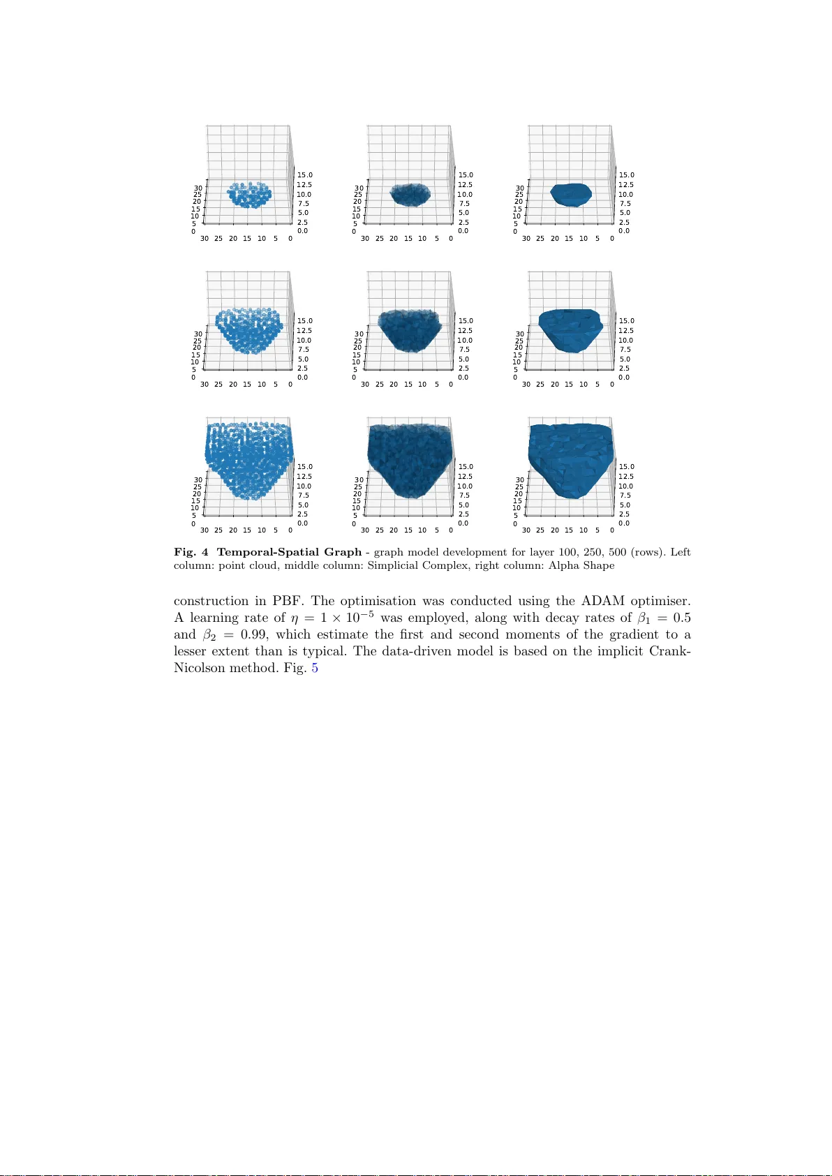
PiGRAND: Ph ysics-informed Graph Neural Diﬀusion for In telligen t Additiv e Man ufacturing Benjamin Uhric h 1,2* , Tim H¨ an tschel 1,2 and Erhard Rahm 1,2 1 Cen ter for Scalable Data Analytics and Artiﬁcial Intelligence Dresden/Leipzig, Germany . 2 Leipzig Universit y , Leipzig, German y . *Corresp onding author(s). E-mail(s): uhric h@informatik.uni-leipzig.de ; Abstract A comprehensiv e understanding of heat transp ort is essential for optimizing v arious mec hanical and engineering applications, including 3D printing. Recent adv ances in machine learning, com bined with ph ysics-based models, ha v e enabled a pow erful fusion of n umerical methods and data-driv en algorithms. This progress is driven by the av ailability of limited sensor data in v arious engineering and scien tiﬁc domains, where the cost of data collection and the inaccessibility of certain measurements are high. T o this end, w e present PiGRAND, a Ph ysics- informed graph neural diﬀusion framew ork. In order to reduce the computational complexit y of graph learning, an eﬃcien t graph construction pro cedure was dev el- op ed. Our approac h is inspired by the explicit Euler and implicit Crank-Nicolson metho ds for mo deling con tinuous heat transp ort, leveraging sub-learning mo dels to secure the accurate diﬀusion across graph nodes. T o enhance computational p erformance, our approach is combined with eﬃcien t transfer learning. W e ev al- uate PiGRAND on thermal images from 3D prin ting, demonstrating signiﬁcant impro vemen ts in prediction accuracy and computational performance compared to traditional graph neural diﬀusion (GRAND) and physics-informed neural net works (PINNs). These enhancemen ts are attributed to the incorp oration of physical principles deriv ed from the theoretical study of partial diﬀerential equations (PDEs) into the learning mo del. The PiGRAND co de is open-sourced on GitHub: https://gith ub.com/bu32loxa/PiGRAND Keyw ords: graph neural diﬀusion, heat transfer, 3D printing, transfer learning, data transformation 1 1 In tro duction Heat transfer or transp ort pla ys a crucial role in engineering and natural sciences. Accurate modeling of heat transp ort in such pro cesses remains a complex task due to the highly dynamic and non-linear nature, esp ecially in real-w orld applications. An understanding of heat transp ort in the context of additiv e manufacturing (AM) is a k ey factor in ac hieving sup erior pro duction quality . Although traditional tec hniques, suc h as the ﬁnite element metho d (FEM) and the ﬁnite v olume metho d (FVM), oﬀer high accuracy by solving PDEs, they often require signiﬁcant computational resources and a considerable amount of preprocessing eﬀort for discretisation. [ 1 – 3 ]. PINNs eﬀectively combine the solution of PDEs with data-driven learning b y incor- p orating w eighting mechanisms to balance the fo cus b etw een data and ph ysical la ws during optimization. F urthermore, they facilitate mesh-free solutions [ 4 ]. How ev er, they may exhibit limitations in terms of scalability due to the curse of dimensionality . This results in high computational costs and slow con v ergence, which pro ve an imped- imen t when dealing with data. In recent years, graph neural net works (GNNs) ha ve emerged as a pow erful to ol for learning on graph-structured data and hav e already sho wn promise in physical sciences [ 5 , 6 ]. Sp eciﬁcally , GRAND oﬀers a framew ork for mo deling pro cesses where information diﬀuses across no des ov er time [ 7 ]. W e prop ose PiGRAND, a nov el framework that extends GRAND to mo del con- tin uous heat transp ort. This is achiev ed through the in tro duction of several key inno v ations, with the ob jectiv es of accelerating the learning pro cess and impro ving accuracy and scalability . In order to establish the foundation for graph learning algo- rithms and to reduce the computational complexity of graph diﬀusion op erations, w e present an eﬃcien t graph construction metho d for transforming thermal images in to graph-structured data representing ph ysical ob jects. F urthermore, a no vel con- nectivit y mo del is suggested to more accurately represent the spatial relationships in high-dimensional data. This mo del is employ ed to ensure accurate diﬀusion across no des with diﬀerent prop erties. T o improv e prediction accuracy , we adopt the concept of PINNs and intro- duce a series of loss terms based on fundamental physical principles related to heat transp ort. In addition, an intelligen t dissipation mo del is in tro duced to regulate the energy transfer at the b oundaries. The utilisation of transfer learning facilitates the application of pre-trained mo dels and knowledge deriv ed from related tasks, thereby reducing the requirement for costly retraining on new data and accelerating the learn- ing process [ 8 ]. T o enhance computational p erformance, we prop ose the utilisation of eﬃcient transfer learning. W e ev aluate PiGRAND on the application of thermal images generated during 3D printing pro cesses. Our results demonstrate a signiﬁcan t impro vemen t in prediction accuracy for heat transfer compared to representativ es of traditional GRAND and PINNs. This improv ement is largely attributed to our k ey inno v ations, whic h allow the mo del to capture the underlying heat transp ort pro cess more eﬀectively . The main contributions of our work are as follo ws: 2 • W e prop ose an eﬃcien t graph construction metho d for transforming thermal image data into graph-structured data. • W e present explicit Euler- and implicit Crank-Nicolson inspired GRAND. • W e extend GRAND by developing t wo sub-learning mo dels (connectivit y and dissipation) and integrating ph ysical principles of heat transp ort as regularization tec hniques for graph learning. • W e show that computational p erformance can b e impro ved by the use of eﬃcient transfer learning. • W e presen t a comprehensive ev aluation demonstrating that our framework is capa- ble of predicting heat transport in 3D-prin ting, outp erforming traditional GRAND and PINNs. The remainder of this pap er is organized as follows. In Section 2, w e review related w ork contributing to graph-based neural diﬀusion models and their applications to ph ysical pro cess simulations. In Section 3, we present the detailed metho dology of PiGRAND and its components, including the data transformation, the sub-learning mo dels and the integration of physical principles as regularization techniques. Section 4 describ es our results in the application of 3D printing. Section 5 presents a com- prehensiv e ev aluation, including the dataset of thermal images, the metrics used for ev aluation and the comparison with GRAND and PINNs. Finally , in Section 6, w e discuss the results and conclude the paper with potential av enues for future researc h. 2 Related W ork This section reviews prior work most relev ant to PiGRAND for heat transp ort mo deling. 2.1 Heat T ransfer Mo delling The ﬁeld of heat transfer represen ts one of the most challenging and widely stud- ied areas within the discipline of computational mechanics. In the con text of 3D prin ting technologies, the app earance of heat conduction is characterised by nonlin- ear b eha viour and is inﬂuenced by a m ultitude of parameters. Scie n tiﬁc Computing enables engineers to sim ulate and predict the b ehaviour of thermal systems across a range of scales, from the comp onent level to that of large-scale infrastructure. This facilitates the design, optimisation and analysis of pro ducts and pro cesses. The devel- opmen t of numerical approximation metho ds has a long history , with the most widely used b eing the FEM and FVM [ 9 – 13 ]. Mukherjee et al. hav e demonstrated their eﬀectiv eness in mo deling heat transfer and ﬂuid ﬂo w for a v ariet y of materials and pro cess parameters, including stainless steel, titanium, and alumin um alloys [ 14 , 15 ]. 3 Extensions of these methods hav e incorp orated multiph ysics coupling, meshfree for- m ulations, and particle-based descriptions to improv e robustness and accuracy in the presence of ev olving domains and localized heat sources [ 16 – 23 ]. The impact of residual stresses on the mechanical prop erties of 3D-prin ted lattices was inv estigated b y Ahmed et al. [ 24 ]. While these techniques pro vide detailed ph ysical insigh t, their computa- tional cost and limited scalability often restrict their applicability in scenarios requiring rep eated simulations, large-scale parameter studies or near-real-time inference. T o address these challenges, recen t work has explored reduced-order and learning-based surrogate models for thermal prediction in AM. Graph-based and meshfree represen ta- tions ha ve gained particular atten tion, as they naturally encode spatial neighborho o ds and lo cal interactions while a voiding the constrain ts of structured meshes [ 25 , 26 ]. Suc h representations enable ﬂexible discretizations of complex geometries and provide a foundation for data-driv en models that can learn heat propagation patterns directly from simulation or exp erimental data. These dev elopments motiv ate the use of graph- structured learning frameworks that preserv e the lo calit y and physical in terpretability of n umerical heat conduction mo dels while signiﬁcantly reducing computational o ver- head. In this con text, diﬀusion-based GNNs oﬀer a promising a ven ue b y aligning message-passing op erations with discretized heat transp ort dynamics. The present w ork builds on this persp ective b y form ulating a PiGRAND model speciﬁcally tailored to thermal modeling in AM. 2.2 Ph ysics-informed Learning Ph ysics-informed learning has emerged as a p ow erful tool for incorporating prior phys- ical knowledge into data-driven mo dels, particularly for systems go verned by PDEs. Raissi et al. introduces PINNs as prominent class of suc h approaches, whic h embed go verning equations, b oundary conditions and constitutive relations directly into the loss function. This form ulation enables neural netw orks to approximate solutions to forw ard and in verse PDE problems while enforcing ph ysical consistency [ 4 ]. Since their in tro duction, PINNs hav e b een successfully applied to a v ariet y of heat trans- fer and ﬂuid ﬂow problems. W essels group dev elop ed the neural particle metho d for computational ﬂuid dynamics and employ ed PINNs for contin uum micromechanics [ 27 , 28 ]. Sev eral studies ha ve demonstrated the p otential of physics-informed learning for thermal mo deling in AM, for example b y integrating conductiv e and conv ective heat transfer equations into neural netw ork training ob jectiv es or b y lev eraging mea- suremen t data for real-time monitoring and anomaly detection [ 29 – 33 ]. In addition, a m ulti-mo del neural net work approach was developed for condition monitoring [ 34 ]. Xu et al. employ ed a transfer learning approach based on PINNs for solving inv erse problems in engineering structures under diﬀerent loading scenarios [ 35 ]. Rasht et al. emplo yed PINNs to solve acoustic wa v e propagation and full wa veform in version problems, demonstrating their meshless ﬂexibilit y and strong inv ersion p erformance across v arying structural complexities. [ 36 ]. Hu et al. introduced stochastic dimension gradien t descent, a no vel training methodology for scaling PINNs to solv e extremely high-dimensional PDEs eﬃciently [ 37 ]. Guo et al. prop osed a data-free predictive sur- rogate mo deling framework, whic h employs tensor-decomp osed conv olutional neural 4 net works to solve high-dimensional parametric problems without training data, achiev- ing remark able computational and memory eﬃciency on ultra large-scale sim ulations [ 38 ]. These approaches highlight the v alue of incorp orating physical constraints to impro ve generalization under limited data and to reduce reliance on purely data-driv en learning. In the presen t work, we build on the conceptual foundations of physics- informed learning while addressing its scalability limitations through a GRAND form ulation that integrates ph ysical regularization in a structurally consistent and computationally eﬃcient manner. 2.3 Diﬀeren tial-Equation-inspired Neural Arc hitectures Diﬀeren tial-equation–inspired neural architectures ha ve emerged as an eﬀective means of introducing physical structure and interpretabilit y into deep learning mo dels. Rather than treating neural netw orks as static input–output mappings, this paradigm views learning as the evolution of a dynamical system, where net work depth corre- sp onds to time discretization and lay er up dates mirror n umerical integration schemes for ordinary or PDEs. This persp ective pro vides a principled foundation for impro ving stabilit y , robustness and generalization in deep mo dels. W einan established a for- mal connection b etw een residual neural netw orks and forward Euler discretizations of dynamical systems, motiv ating the design of architectures inspired b y classical time-in tegration metho ds [ 39 , 40 ]. Shen et al. extended this idea b y incorp orating a bac kward Euler formulations as implicit scheme, to enhance stability and allow for deep er netw orks without degradation[ 41 ]. He et al. emplo yed the use of ODE-inspired net work design for single image sup er-resolution. The authors propose several net- w ork arc hitectures based on Runge-Kutta methods [ 42 ]. Similar principles ha ve also b een adopted in ODE and PDE-inspired architectures, where the structure of motion, diﬀusion, transp ort or reaction equations informs the design of con volutional and recurren t neural netw orks [ 43 – 47 ]. Khoshsirat and Kambhamettu developed an ODE transformer netw ork [ 48 ]. A k ey adv antage of diﬀerential-equation–inspired mo dels is their abilit y to enco de inductiv e biases that align learning dynamics with kno wn ph ys- ical pro cesses. By b orrowing concepts suc h as stabilit y conditions, consistency and discretization error from n umerical analysis, these architectures oﬀer greater inter- pretabilit y and improv ed training b eha vior compared to purely data-driven designs. This is particularly relev an t for physical systems c haracterized by diﬀusive dynamics, where information propagation is inheren tly lo cal and gov erned b y conserv ation prin- ciples. These ideas form the conceptual basis for diﬀusion-based learning on graphs, in which message passing can b e interpreted as a discrete approximation of contin uous dif- fusion pro cesses ov er irregular domains. By extending diﬀerential-equation–inspired arc hitectures to graph-structured data, GRAND models provide a natural and physi- cally meaningful framework for mo deling heat transp ort in complex geometries. The presen t work lev erages this foundation b y adopting b oth explicit and implicit diﬀu- sion sc hemes within a graph neural netw ork to achiev e stable and scalable thermal predictions. 5 2.4 Graph Neural Net w orks GNNs are designed to operate on graph-structured data, where en tities are represen ted as no des and in teractions are enco ded through edges. Unlike traditional neural net- w orks that work with grid-like data suc h as images or sequences, GNNs are tailored to capture the complex, non-Euclidean structures found in so cial net works, molecu- lar graphs and knowledge graphs [ 49 – 53 ]. This form ulation is particularly w ell suited for physical systems, as graphs naturally reﬂect spatial discretizations, neighborho o d in teractions and irregular geometries commonly encoun tered in scientiﬁc and engineer- ing applications. By aggregating information from local neighborho o ds, GNNs enable the modeling of complex dep endencies that are diﬃcult to c apture with grid-based arc hitectures. In recen t years, GNNs ha ve b een increasingly applied to physics-based problems, including particle interactions, ﬂuid dynamics and surrogate mo deling of PDEs. Sc hlomi et al. emplo yed a range of applications of GNNs within the con- text of particle physics [ 54 ]. In these contexts, message-passing mec hanisms can b e in terpreted as lo calized information exc hange analogous to numerical stencils, making GNNs a ﬂexible alternativ e to traditional mesh-based solvers. Gao et al. dev elop ed a no vel discrete PINN framew ork based on graph conv olutional netw ork and v ariational structure of PDEs to solv e forw ard and in verse PDEs [ 55 ]. Despite their ﬂexibil- it y , conv entional GNN architectures typically rely on ﬁxed message-passing rules and shallo w propagation depths, which can limit their ability to represen t con tinuous diﬀu- sion pro cesses o v er extended spatial or temp oral scales. In ph ysical systems gov erned b y heat transp ort, this can lead to ov ersmo othing, n umerical instability or insuﬃ- cien t represen tation of long-range thermal in teractions. These limitations highlight the need for graph-based mo dels that explicitly incorp orate diﬀusion dynamics into their arc hitectural design. 2.5 Graph Neural Diﬀusion Cham b erlain et al. introduces GRAND mo dels extending standard GNNs by inter- preting message passing as a discretized diﬀusion pro cess on a graph. This p ersp ective establishes a direct connection b et ween graph learning and the n umerical solution of PDEs, enabling the systematic design of stable and interpretable architectures. A tw o o d and T owsley introduced diﬀusion-based graph con volutions, while more recent approac hes hav e formalized GNNs as explicit or implicit time discretizations of an underlying diﬀusion equation [ 56 ]. A k ey con tribution of diﬀusion-based graph mo d- els is their ability to mitigate common challenges in deep graph learning, such as o versmoothing and v anishing gradien ts, b y lev eraging w ell-established n umerical in te- gration schemes. Explicit formulations oﬀer computational eﬃciency and simplicity , whereas implicit sc hemes pro vide improv ed stability and allo w for deep er propagation without loss of expressiv e p ow er [ 7 ]. These prop erties hav e led to strong p erformance across a range of graph learning benchmarks and ha ve enabled applications in domains suc h as climate mo deling and en vironmental prediction [ 57 , 58 ]. Building on this foundation, Thorp e et al. hav e incorp orated source terms and nonlinear dynamics to further enhance expressiveness [ 59 ]. Ho wev er, existing GRAND mo dels are largely 6 dev elop ed and ev aluated on b enchmark datasets, missing the in tegration of domain- sp eciﬁc physical constraints. In contrast, the present work in tro duces PiGRAND, a ph ysics-informed graph neural diﬀusion framew ork tailored to heat transp ort mo d- eling in AM. By em b edding ph ysically motiv ated regularization terms deriv ed from heat conduction theory and introducing sub-learning mo dels for connectivity and dis- sipation, PiGRAND extends diﬀusion-based graph learning. This work represents a signiﬁcan t extension of the ideas initially set forth in [ 60 ]. The conference pap er intro- duces the explicit inspired GRAND mo del but lacks any ev aluation and only provides preliminary results. In con trast, the prop osed work signiﬁcantly extends the ﬁndings b y presenting the implicit Crank-Nicolson-inspired GRAND model, incorp orating a transfer learning strategy based on a foundation model to predict heat transp ort on other comp onents based on diﬀeren t material with muc h greater eﬃciency . Addition- ally , it oﬀers a comprehensive ev aluation of the results, demonstrating the adv an tages compared to PINNs and traditional GRAND. The initial mo del from [ 60 ], was also used in further work to generate temp erature features as part of a multimodal graph transformer approach [ 61 ]. 3 Metho dology Our prop osed framework features a graph construction metho d that transforms ther- mal data into graph-structured data, and our PiGRAND mo del. The theoretical bac kground of these metho ds is given b elo w. 3.1 Data T ransformation A graph G = ( V , E ) is a data structure consisting of a set of v ertices V = { 1 , . . . , N } and a set of edges E ⊆ V × V . If the graph is em b edded in Euclidean space, i.e. there is a map ι : V → R n , the Euclidean distance of v ertex positions ι ( i ) ∈ R n , i = 1 , . . . , N giv es rise to a distance function on V . As a shorthand notation, w e write v i := ι ( i ). W e consider ph ysical ob jects and therefore alwa ys ha ve n = 3. An arbitrary spatial structure in R 3 can b e approximated using a simplicial 3-complex. F or eac h lay er in a prin ting job, the ob jective is to represent the partial ob ject prin ted up to the resp ective la yer by a simplicial complex, such that a) the shap e of the complex closely resembles the shap e of the part, and b) the dynamics of the heat distribution in the part can b e mo deled by a diﬀusion process on the underlying graph, i.e. the graph whose vertices and edges are given by the 0- and 1-simplices in the complex. Thermal images of the surface are taken p erio dically during the prin ting process, allo wing for detecting the shap e of each lay er b y taking an empirical threshold. Stacking this information for all la yers, we obtain a 3-dimensional set of pixels, representing the shap e of the ob ject. 3.1.1 Graph Construction from Thermal Images F or a detailed description of the underlying sensor data and thermal images, see [ 32 ]. W e asso ciate the pixels of a thermal image with p oints on a plane in R 3 , that is parallel to the (x, y)-plane and con tains the current lay er of the printing job. A p oint is assumed to be part of the printed ob ject, if the temp erature v alue of the associated 7 pixel is ab ov e an empirical threshold. If this is the case, the point is added to a point cloud in R 3 , b y attaching a third component to the pixel co ordinates, enco ding the v ertical p osition of the la yer. The empirical threshold is set to 423.15 Kelvin, whic h is appro ximately the temp erature of the built plate and the unmelted metal p o wder. In order to build the simplicial complex, a representativ e subset needs to b e selected from the comp osite p oin t cloud. T o this end, w e make use of the pruning method describ ed in [ 62 ], which is based on iteratively remo ving the p oin t with the highest scale-in v ariant density (SID). Since our p oint cloud is a set in R 3 instead of a plane, S1: P oint Cloud S2: Pruning S3: Delaunay T riangulation S4: Alpha Shape S5: Simplicial 3-Complex Fig. 1 Graph Construction Algorithm - Step 1: Generating p oint cloud, Step 2: Pruning method, Step 3: Delaunay triangulation, Step 4: Alpha shape, Step 5: Simplicial 3-complex. w e adapt the SID, b y replacing the r -density with the 3-dimensional analogue d r ( v i ) = # {∥ v j − v i ∥ 2 < r : 1 ≤ j ≤ N , i  = j } 4 3 π r 3 , (1) whic h is the num b er of data p oints in the r -ball around v i , divided by the v olume of the ball. The scale-inv ariant density is deﬁned as the in tegral o ver all r -densities: d ( v i ) = Z ∞ 0 d r ( v i ) dr (2) 8 and by a similar calculation as in [ 62 ], we see that: d ( v i ) =  8 3 π  − 1 X j  = i   v i − v j   − 2 2 . (3) In each step, the point with the highest spatial redundancy (measured b y the SID) is remo ved. The resulting subset is relativ ely homogeneously distributed o ver the in terior of the p oint cloud, but con tains many b oundary p oin ts, as their surrounding is partially v oid, resulting in a low er SID. This is desirable, as the b oundary p oints deﬁne the shap e of the printed ob ject. F or building the graphs represen ting the partially printed ob ject, we iterate ov er the num b er of lay ers n , ranging from 1 to the total n umber M of lay ers in the printing job. F or each n , the pruned set of points from the previous step is considered together with the p oints from the n -th lay er. W e restrict pruning to points from the top k lay ers ( k ≪ M ), th us the representation for the ﬁrst n − k lay ers is inherited. A simplicial complex is constructed from the set of pruned p oints, using Delaunay triangulation [ 63 ]. The printed part m ust not necessarily be conv ex, but the shap e produced by the Delaunay triangulation alw ays is. T o extract only the simplices that are within the b oundary of the printed part, w e use an alpha shap e [ 64 ] to determine the h ull of the p oint cloud. Remo ving the simplices that are not encased by the alpha shap e, w e end up with a simplicial 3- complex that resembles the shap e of our prin ted ob ject (see Fig. 1 ). The v ertices and edges of this complex are used to deﬁne a graph. Moreo ver, the option exists to b ypass the pruning method when creating a simplicial complex based on the original point cloud. How ever, there would be a trade-oﬀ in terms of computational complexity . The vertices are categorized based on spatial p osition: 1. vertices in the lo west lay er are assigned to the b ottom b oundary class 2. vertices in the surface lay er are assigned to the top b oundary class 3. vertices that are part of a surface of the alpha shape, but neither in the top- nor b ottom b oundary are assigned to the side b oundary class 4. vertices that are not part of either of these classes are assigned to the interior class C i = C ( v i ) denotes the class of the vertex v i , i = 1 , . . . N . 3.2 Numerical Mo dels for the Graph Diﬀusion Pro cess F ormally , the heat equation, which describ es the heat diﬀusion process in a homoge- neous b o dy and the initial-b oundary v alue problem is given by ∂ ∂ t T ( x, t ) = α ∆ T ( x, t ) , x ∈ Ω , t ∈ [0 , T ] (4) T ( x, t 0 ) = T 0 , x ∈ Ω (5) ∂ ∂ n T ( x, t ) = T B , x ∈ Ω , t ∈ [0 , T ] (6) 9 where ∂ ∂ t is the deriv ative w.r.t. time, α is a conductivity parameter and ∆ is the Laplace operator in the spatial domain. F or computational mo deling of the heat trans- fer process, we must discretise Eq. ( 4 ) b oth in space and in time. In the con text of a diﬀusion pro cess on an ob ject that is represented b y a graph, the natural replacement for the Laplacian op erator is the graph Laplacian matrix L , whic h is deﬁned as L := D − A (7) where A is the adjacency matrix containing the edge weigh ts for pairs of vertices in a ﬁxed enumeration, and D is the degree matrix, i.e. the diagonal matrix whose entries are the sum of the w eights of adjacent edges for eac h v ertex. Regarding the time deriv ative, the practical replacement is found by considering dif- ference quotients instead of the diﬀeren tial. T o this end, the time domain  0 , T  is sub divided into small interv als of some length δ t ≪ T , and the discrete ev aluation p oin ts are chosen as t n = n δt, n = 0 , 1 , . . . , T /δ t . When approximating the time deriv ative at a lattice p oint t n , one m ust decide betw een selecting the diﬀerence quo- tien t w.r.t. the previous or w.r.t. the subsequent lattice p oint. Dep ending on this decision, the appro ximation of the heat transfer pro cess is either describ ed by an explicit scheme motiv ated by the T aylor series for a solution of the homogeneous heat equation Eq. ( 4 ): T ( x, t + δ t ) = ∞ X j =0 1 j !  ∂ ∂ x  j T !  x, t  ( δ t ) j (8) = T ( x, t ) + ∞ X j =1 1 j !  ∂ ∂ x  j T !  x, t  ( δ t ) j (9) Note that for a solution of the homogeneous heat equation, its deriv ative w.r.t. t is again a solution of the heat equation, since 0 = ∂ ∂ t  ˙ T − α ∆ T  = ¨ T − α ∆ ˙ T . Hence, w e can replace  ∂ ∂ x  j b y ( α ∆) j in the T aylor series. Approximating α ∆ by L ( T ), w e obtain: T ( x, t + δ t ) ≈ T ( x, t ) + ∞ X j =1 1 j !  L ( T ) j T   x, t  ( δ t ) j (10) As can be seen, using only the ﬁrst t wo terms of the T aylor series : T n +1 − T n δ t = LT n (11) ⇐ ⇒ T n +1 = T n + δ tLT n (12) for the forw ard step (ev aluated at time-step n ), or an implicit scheme T n +1 − T n δ t = LT n +1 (13) 10 ⇐ ⇒  Id − δ tL  T n +1 = T n (14) ⇐ ⇒ T n +1 =  Id − δ tL  − 1 T n (15) when choosing the backw ard step (ev aluated at time-step n + 1) and in tro ducing the iden tity matrix Id. These metho ds for solving PDEs numerically are kno wn as the forw ard- and the backw ard Euler method. The LHS in Eq. ( 11 ) and Eq. ( 13 ) can b e in terpreted as an estimate for the deriv ative at the midp oin t b et ween times t n and t n +1 . On the other hand, the RHSs are the Laplacians at the times t n and t n +1 . A third sc heme can b e obtained b y com bining the tw o previous sc hemes, taking the mean of the Laplacian at t n and at t n +1 , in order to estimate the Laplacian at the midp oint, T n +1 − T n δ t = 1 2  LT n + LT n +1  (16) ⇐ ⇒  Id − 1 2 δ tL  T n +1 =  Id + 1 2 δ tL  T n . (17) ⇐ ⇒ T n +1 =  Id − 1 2 δ tL  − 1  Id + 1 2 δ tL  T n . . (18) This is known as the Cr ank-Nic olson scheme. Since L has non-p ositive sp ectrum,  Id − δ tL  − 1 and  Id − ( δ t/ 2) L  − 1 exist ∀ δ t > 0, and th us the implicit step and the Crank-Nicolson step b oth hav e a unique solution. The explicit metho d is eﬃcient to compute (note that L is sparse and the num b er of neighbours of a no de in a mes h is constan t for diﬀerent sizes of the mesh, so the cost of Eq. ( 12 ) is linear in the n umber of nodes), but it requires c ho osing a small step size δ t of the order ( δ x ) 2 , otherwise the numerical solutions may explo de [ 65 ]. In contrast, the implicit scheme and the Crank-Nicolson scheme are numerically stable for an y c hoice of step size. 3.3 Neural Diﬀusion Mo dels on Graphs The utilisation of numerical mathematics is fundamental to the creation of graph learn- ing mo dels that are capable of discretising and approximately solving the con tinuous heat equation. Due to non-equidistan t vertices in the graph, inhomogeneous conduc- tivit y dep ending on the temp erature and a random laser tra jectory in the 3D prin ting pro cess, it is practically imp ossible to determine the correct parameters and b ound- ary conditions for mo deling the heat transp ort pro cess purely numerically . Instead w e prop ose a more complex mo del to predict the heat transfer, incorp orating real mea- suremen t data as well as kno wn prop erties of diﬀusion pro cesses. Revisiting Eq. ( 4 ), w e in tro duce a lo cal state-dep endence to α , and an additional dissipation term Q , to accoun t for heat loss at the boundary: ˙ T ( x, t ) = α  T ( x, t )  ∆ T ( x, t ) − Q  x, T ( x, t )  (19) F or a discrete approximation of the heat pro cess on a graph, we consider the explicit sc heme Eq. ( 12 ) and the Crank-Nicolson scheme Eq. ( 18 ), and extend both b y intro- ducing the dissipation term Q on the RHS, whic h dep ends on the temp erature state 11 T n . F urthermore, in the neural diﬀusion model, w e allo w for temp erature-dep enden t conductivit y , whic h implies that the graph Laplacian L is a function of the temp er- ature state. W e build these functional dep endencies, such that only the lo cal graph structure and lo cal temp erature v alues inﬂuence the resp ective en tries of L and Q . F or a single v ertex v i , we assert that the lo cal information is given b y the temp era- ture T n ( v i ), the vertex class C ( v i ) and the scale inv arian t density d ( v i ). F or an edge b et ween tw o adjacent vertices v i , v j , we deﬁne the lo cal information as the vertex dis- tance ϱ ij = ∥ v i − v j ∥ 2 , together with the lo cal information for each of the t w o vertices. The graph Laplacian is then constructed as giv en b y Eq. ( 7 ), but the adjacency matrix A =  a ij  i,j =1 ,...,N is replaced b y a state-dep enden t adjacency b A , deﬁned as b A = ( 0 , a ij = 0 , c ij , a ij  = 0 , (20) where the non-zero entries c ij of b A are estimated by a learnable function c ij ( T n ) = φ  ϱ ij , T n ( v i ) , T n ( v j ) , C ( v i ) , C ( v j ) , d ( v i ) , d ( v j )  (21) whic h is realised b y a single-hidden-lay er neural netw ork of width 256. Finally , for assem bling the Laplacian, the degree matrix D of A is replaced accordingly b y b D whic h is computed w.r.t. to b A , such that we obtain the state dep enden t Laplacian b L ( T n ) := b D ( T n ) − b A ( T n ). In a similar fashion, the i -th entry of the dissipation vector Q ( T n ) =  Q i ( T n )  i should only dep end on the lo cal prop erties of v i , i.e. T n ( v i ), C ( v i ), d ( v i ). This motiv ates mo delling Q i ( T n ) by a function Q i ( T n ) = ψ  T n ( v i ) , C ( v i ) , d ( v i )  (22) whic h again is implemented as a single-hidden-lay er netw ork of width 256. Th us, in the explicit neural heat mo del, the diﬀusion process is computed recursively b y the mo del equation T n +1 ( T n ) = T n + δ t b L ( T n ) T n − δ t Q ( T n ) (23) and in the neural heat mo del based on the Crank-Nicolson method, the adapted model equation is giv en by T n +1 ( T n ) =  Id − 1 2 δ t b L ( T n )  − 1  Id + 1 2 δ t b L ( T n )  T n − δ t Q ( T n ) . (24) These mo dels con tain the trainable submo dels φ and ψ determining b L and Q . T raining this kind of mo del presents sev eral obstacles. W e identify the follo wing c hallenges: 12 1. Using the mo del to predict changes in surface temp erature requires kno wing the initial state T 0 for all v ertices, including those that cannot be observed. The limited observ abilit y of vertices lik ely leads to an underdetermined optimization problem, whic h raises doubts ab out the mo del’s abilit y to accurately represen t the in ternal heat state. 2. The recursive nature of the model, without the p ossibility to correct the interme- diate temp erature state due to limited information, facilitates the comp ounding of errors and hinders the training pro cess. 3. The lo cal character of the mo del, where in eac h step only the state in the direct neigh b ourho o d aﬀects the temp erature change at a vertex, leads to v anishing gradien ts for the temp erature v alues at vertices that are not in proximit y to the surface lay er. T o address these issues, we deviate from the standard data-driven training process for machine learning mo dels in the following manner: • T o o v ercome the problem of the unknown initial states, w e start at the ﬁrst la yer, where the complete state can b e observed. W e train the diﬀusion mo del on the initial lay er, until an acceptable accuracy is ac hieved. Then, we use the obtained mo del to predict the diﬀusion pro cess for the now hidden v ertices in the ﬁrst lay er, until the start of the prin ting process for the sec- ond la yer. No w, we use the predicted in ternal state as the hidden state for predictions on the second lay er, and up date the hidden temp erature v alues for each time step, according to the mo del prediction. Again, we train the mo del on the ﬁrst and second lay er, until acceptable precision is reac hed, b efore starting to train the model on the third lay er. This metho d of grad- ually increasing the n umber of lay ers helps us obtaining consistent internal states, which are the foundation for precise mo del predictions. • Besides the standard loss function that compares the mo del prediction to the observed data, w e introduce additional regularizing loss functions, based on physical and mathematical information ab out the diﬀusion pro cess. Mo d- els that incorp orate equations describing ph ysical systems as regularization functions in the training of neural netw orks are kno wn as PINNs. This approac h restricts our mo del b y in tro ducing an additional loss to dynamics that are inconsisten t with real diﬀusion processes. • In order to introduce a dep endency b et ween vertices with larger distance in the graph, w e must increase the discrete time horizon in each training step. T o this end, we subdivide eac h time step in our training data into multiple steps for the numerical appro ximation. Then, if one training step consists of 13 k steps of the numerical approximation, paths of length up to k are consid- ered in the training pro cess and therefore vertices in the lo wer part of the graph can inﬂuence the state at the surface. 3.4 Regularizing Loss F unctions W e discuss in detail the deriv ation of the previously mentioned regularizing loss func- tions. F or the connectivity mo del φ , it is known from the discretization of the contin uous Laplacian, that the connectivit y of tw o adjacent vertices should b e prop ortional to the in verse square of their distance, ϱ − 2 ij . Assuming φ ( ϱ ij ) = τ ϱ − 2 ij (k eeping all other parameters constant), it follo ws φ ′ ( ϱ ij ) = − 2 τ ϱ − 3 ij , and thus φ ′ ( ϱ ij ) φ ( ϱ ij ) = − 2 ϱ − 1 ij , which is indep endent of the scale τ . Therefore, the ﬁrst regularizing loss term is given by: L φ = X i,j : i ∼ j  φ ′ ( ϱ ij ) φ ( ϱ ij ) −  − 2 ϱ − 1 ij   2 (25) L φ = X i,j : i ∼ j φ ( ϱ ij ) − 1 ϱ 2 ij ! 2 (26) whic h ensures consistency of the edge weigh ts with the distances of the connected v ertices. F urthermore, dissipation can only occur at the boundary , so ψ = 0 is required for interior p oin ts, motiv ating the loss: L ψ = X i : C ( v i )=int. ψ ( T n ( v i ) , C ( v i ) , d ( v i )) 2 (27) Using knowledge from the theoretical study of PDEs, it is also p ossible to mak e state- men ts ab out the temporal ev olution of the heat state. First, the total thermal energy in the b ody can only change because of heat transfer at the b oundary , whic h in the discrete mo del has the equiv alent P i T n +1 ( v i ) = P i  T n ( v i ) − Q n ( v i )  . Therefore, we prop ose the loss function L heat = X i  T n +1 ( v i ) − T n ( v i ) + Q n ( v i )  ! 2 . (28) Another well known prop ert y of the evolution of heat distribution is the maximum principle (see for example [ 66 ], § 2.3.). F or our purp ose, it suggests that the temp erature at a vertex is w ithin the range giv en b y the minimum and maximum ov er its previous temp erature and the temp eratures of connected vertices. This is expressed by the 14 regularizing loss terms: L max = X i max  0 , T n +1 ( v i ) − max( M )  2 (29) L min = X i max  0 , min( M ) − T n +1 ( v i )  2 (30) M =  T n ( v i ); T n +1 ( v j ) , v j ∼ v i  F urthermore, a potential energy for the heat distribution can b e deﬁned by E ( T , t ) = Z U  T ( x, t ) − T ( t )  2 dx (31) F or the time-diﬀeren tial of this energy , one can compute: ˙ E ( T , t ) =2 Z U  T ( x, t ) − T ( t )  ˙ T ( x, t ) dx =2 α Z U  T ( x, t ) − T ( t )  ∆ T ( x, t ) dx =2 α  Z ∂ U  T ( x, t ) − T ( t )   ∇ T ( x, t ) · ν  dS | {z } energy loss from dissipation − Z U |∇ T ( x, t ) | 2 dx | {z } ≥ 0  (32) Assuming dissipation is relatively small, it should roughly hold that ˙ E ≤ 0, so E ( T n +1 ) ≤ E ( T n ). Thus, we introduce another loss term: L energy = max  0 , b E ( T n +1 ) − b E ( T n )  (33) where b E ( T n ) = 1 N X i  T n ( v i ) − T n  2 with T n = 1 N X i T n ( v i ) (34) is the discrete approximation of the potential energy . F or training the mo del, the regularizing loss functions L φ , L ψ , L heat , L min , L max , and L energy , as w ell as the prediction loss L data = X i : C i =top  T n +1 ( v i ) − T ( data ) n +1 ( v i )  2 (35) are added using appropriate weigh ts, and the descen t algorithm seeks to ﬁnd a min- im um for the sum, i.e. a mo del state that ﬁts the data without violating kno wn 15 D a t a loss M a t h ema t ic al c on c lu sion s Ph y sic al p rin c ip les … gr ad ien t - f low alo n g ed g es               Input Hidd en la y er Hidd en la y er O u tp u t   󰇛   󰇜   󰇛   󰇜            󰇛   󰇜 d 󰇛   󰇜 Op t imiz a t ion Up d a t e Exp lic it Eu ler : Im p lic it C r an k Nic olson : Ph y si cs - i n f or me d g r ap h neur al di f f usi on Gr ap h c on s t ru c t ion / D a t a t r an s f or ma t ion f r om t h er mal imag es 󰅀  Fig. 2 Flow c hart - Graph construction and physics-informed graph neural diﬀusion prop erties of heat diﬀusion. This restricts the admissible set of solutions, th us mitigat- ing the problem of underdetermination, and the regularizing loss functions also regard v ertices that are disconnected from the surface and therefore not captured b y L data . A ﬂow chart of the complete framework, including graph construction and PiGRAND, can b e found in Fig. 2 . Fig. 3 Geometry of Printed Ob jects - Photographs of high quality comp onents, strongly deformed component P9 and CAD models 16 P h 0 [mm] α [ ° ] l 1 [mm] l 0 [mm] h 1 [mm] Material 4 10 70 20 6.7 18.27 Stainless Steel 7 10 70 25 8.3 22.94 Stainless Steel 9 10 50 25 8.3 9.95 Stainless Steel 7M 10 70 25 8.3 22.94 Nick el-based Alloy T able 1 Comparison of the measures of the 3D-printed ob jects P4, P7, P9 and P7M 4 Results in the Application of P o wder Bed F usion The following section presents the results of PiGRAND and oﬀers a comprehensive ev aluation utilising a range of metrics. This analysis is designed to assess the p er- formance, accuracy and ov erall eﬀectiveness of the prop osed metho d. Additionally , comparisons with state-of-the-art metho ds will b e provided to highlight the relative strengths and potential areas for impro vemen t in PiGRAND. This ev aluation will pro- vide insights into the robustness, scalabilit y and practical applicabilit y of the mo del across diﬀerent datasets and scenarios. These include three printed stainless steel pyra- mids: t wo of go o d qualit y and one of po or quality and one of go o d qualit y made from a nick el-based alloy (see Fig. 3 and T able 1 ). 4.1 Heat T ransfer Prediction based on Thermal Images In order to predict heat transfer in PBF, the prop osed model was trained for a total of 4500 iterations across 500 print lay ers, based on the constructed graph framew ork. The time steps used are measured from the beginning of the current lay er to the end. The discrete heat state predictions dep end on the n umber of thermal images, whic h are generated at a frequency of 3 Hz. This means that one predictiv e timestep corresponds to 1 3 s. The time required to prin t eac h la yer v aries due to the increasing surface area as the comp onent builds up. T o enhance the discrete time resolution in eac h training step, w e subdivide each timestep in our training data into four smaller steps for n umerical appro ximation. This allows vertices in the lo wer part of the graph to inﬂuence the state at the surface. The initial state Eq. ( 5 ) is tak en from the ﬁrst lay er of the p yramid (with previous lay ers acting as supp orting material), where the complete state is observ able. This approach addresses the problem of unknown initial states. F or eac h subsequent la yer, the last predicted temp erature state of the previous lay er serv es as the hidden initial state. The heat ﬂux applied by the laser, mo deled as b oundary condition on the top surface, is represented by the Gaussian mo del q = I e − dη , where I is the in tensity , d is the distance, and η is the decay factor. Both I and η are data-driven parameters ﬁtted during training. Due to the random nature of the laser tra jectory , a laser detection metho d is emplo yed. The Neumann b oundary conditions Eq. ( 6 ), which describ e radiation, are approximated using our dissipation mo del. The constructed graph is illustrated in Fig. 4 . The temp oral graph illustrates the nece ssary steps of the graph construction process (p oin t cloud, simplicial complex and alpha shape) for print la yers 100, 250 and 500. In particular, the graph undergoes substantial mo diﬁcations with the addition of eac h lay er. It is imp erative to consider these changes in order to accurately capture the transient heat ﬂow that o ccurs during the lay er-by-la y er 17 0 5 10 15 20 25 30 0 5 10 15 20 25 30 0.0 2.5 5.0 7.5 10.0 12.5 15.0 0 5 10 15 20 25 30 0 5 10 15 20 25 30 0.0 2.5 5.0 7.5 10.0 12.5 15.0 0 5 10 15 20 25 30 0 5 10 15 20 25 30 0.0 2.5 5.0 7.5 10.0 12.5 15.0 0 5 10 15 20 25 30 0 5 10 15 20 25 30 0.0 2.5 5.0 7.5 10.0 12.5 15.0 0 5 10 15 20 25 30 0 5 10 15 20 25 30 0.0 2.5 5.0 7.5 10.0 12.5 15.0 0 5 10 15 20 25 30 0 5 10 15 20 25 30 0.0 2.5 5.0 7.5 10.0 12.5 15.0 0 5 10 15 20 25 30 0 5 10 15 20 25 30 0.0 2.5 5.0 7.5 10.0 12.5 15.0 0 5 10 15 20 25 30 0 5 10 15 20 25 30 0.0 2.5 5.0 7.5 10.0 12.5 15.0 0 5 10 15 20 25 30 0 5 10 15 20 25 30 0.0 2.5 5.0 7.5 10.0 12.5 15.0 Fig. 4 T emp oral-Spatial Graph - graph mo del developmen t for lay er 100, 250, 500 (ro ws). Left column: point cloud, middle column: Simplicial Complex, righ t column: Alpha Shap e construction in PBF. The optimisation was conducted using the ADAM optimiser. A learning rate of η = 1 × 10 − 5 w as emplo yed, along with decay rates of β 1 = 0 . 5 and β 2 = 0 . 99, which estimate the ﬁrst and second moments of the gradient to a lesser extent than is t ypical. The data-driven mo del is based on the implicit Crank- Nicolson metho d. Fig. 5 provides heat transfer snapshots at key stages of the prin ting pro cess, sp eciﬁcally at print lay ers 100, 250, 350 and 500. This pro vides insigh t in to ho w the model ev olves to trac k the heat transfer dynamics at diﬀerent stages. In this w ay , an insigh t c an b e gained into the wa y in which the mo del a dapts to the ongoing thermal pro cesses within the PBF environmen t. PiGRAND pro vides an in tuitiv e visual represen tation of the heat transfer mo deling throughout the printing process, allowing a deep er understanding of the temp oral heat distribution and the inﬂuence of the increasing num b er of la yers. 18 x 0 5 10 15 20 25 30 y 0 5 10 15 20 25 30 z 0 2 4 6 8 10 12 14 300 400 500 600 700 800 900 T[K] x 0 5 10 15 20 25 30 y 0 5 10 15 20 25 30 z 0 2 4 6 8 10 12 14 300 400 500 600 700 800 900 T[K] x 0 5 10 15 20 25 30 y 0 5 10 15 20 25 30 z 0 2 4 6 8 10 12 14 300 400 500 600 700 800 900 T[K] x 0 5 10 15 20 25 30 y 0 5 10 15 20 25 30 z 0 2 4 6 8 10 12 14 300 400 500 600 700 800 900 T[K] Fig. 5 4D-Heat T ransp ort Prediction - Heat transp ort evolution for lay er 100, 250, 350, 500. As time progresses, the comp onen t’s temp erature increases, reaching a maximum at the upp er portion and subsequently declining tow ards the base. 5 Ev aluation In this section, w e conduct a comprehensiv e ev aluation of the proposed metho d, focus- ing on prediction accuracy , performance and inﬂuence of our prop osed regularization tec hniques. 5.1 Prin t La yer Prediction T op Surface T o ev aluate the predictive accuracy of PiGRAND, a comprehensive comparativ e anal- ysis w as conducted b etw een the observ ed heat state and the predicted heat state for prin t la yer 232. These results w ere benchmark ed against those obtained using a PINN [ 32 ] and traditional GRAND. Notably , GRAND predictions w ere based solely on the prediction loss Eq. ( 35 ) without any regularization, thereby providing a baseline for comparison (see Fig. 6 ). In addition to the prediction of the top surface t = 7 s , the 19 0 10 20 30 Data 300 400 500 600 700 T[K] 0 10 20 30 PINN 300 400 500 600 700 T[K] PINN 0 10 20 30 40 50 a b s 0 10 20 30 GRAND 300 400 500 600 700 T[K] GRAND 0 10 20 30 40 50 a b s 0 5 10 15 20 25 30 0 10 20 30 PiGRAND 300 400 500 600 700 T[K] PiGRAND 0 10 20 30 40 50 a b s Fig. 6 Heat T ransp ort Prediction and Error Plots – A comparison of the heat transp ort prediction for prin t lay er 232 ( t = 7s) with a PINN, GRAND, PiGRAND and the real measurement data. 0 5 10 15 20 t[s] 1 0 5 1 0 4 1 0 3 1 0 2 r GRAND PiGRAND PINN Fig. 7 Relative Error - Comparison of ϵ r between GRAND, PiGRAND and PINN o ver the entire printing layer 232 for each timepoint. 20 PINN GRAND PiGRAND 1 N T P N T k =0 ϵ r 0.041 0.003 0.001 T able 2 Comparison of the mean v alue of ϵ r between PINN, GRAND and PiGRA ND, where N T is the num ber of time p oints during prin ting la yer 232. absolute error can b e seen: ϵ abs = | ( T 21 ( v i ) − T ( data ) 21 ( v i ) | i ∈ top (36) In order to ev aluate the whole printing lay er for all three mo dels, we prop ose the relativ e error: ϵ r = r 1 N P i : C i =top  T n +1 ( v i ) − T ( data ) n +1 ( v i )  2 1 N P i : C i =top  T ( data ) n +1 ( v i ) − 1 N P i T ( data ) n +1 ( v i )  2 (37) The analysis included all predicted time p oints during the prin ting of lay er 232, sho wcasing the capability of PiGRAND to accurately capture b oth spatial and temp o- ral heat dynamics. The comparative results highlight PiGRAND’s superior ability to handle complex heat transfer pro cesses, demonstrating more robust and precise pre- dictions compared to the PINN and GRAND approaches (see Fig. 7 and the mean in T able 2 ). Fig. 7 illustrates the temp oral ev olution of the relativ e error ϵ r for GRAND, PiGRAND and PINN. The results demonstrate a clear adv antage of PiGRAND in terms of predictive accuracy and temp oral stabilit y . While GRAND exhibits p erio dic spik es in error asso ciated with lo cal transient phenomena, PiGRAND signiﬁcantly reduces b oth the magnitude and frequency of these spikes. It maintains a consistently lo wer error throughout the simulation highligh ting its enhanced robustness and gen- eralization. PINNs, in c on trast, exhibit higher and more stable error lev els, indicating reduced sensitivity to temp oral transien ts but also a lo wer o verall accuracy . 5.2 Explicit Euler vs Implicit Crank-Nicolson W e compare the predictions of our tw o prop osed GRAND mo dels, inspired b y the explicit Euler and the implicit Crank-Nicolson methods. It is w ell established in n umer- ical analysis that implicit solvers for PDEs oﬀer signiﬁcant adv an tages in stabilit y , particularly for stiﬀ problems. Ho wev er, this comes at the cost of increased computa- tional eﬀort. T o assess the accuracy of both approac hes, w e employ the relativ e error Eq. ( 37 ) betw een the data and the prediction on the top surfaces and the sum of Eq. ( 31 ), Eq. ( 29 ), Eq. ( 33 ) and Eq. ( 28 ): ˆ L Energy = L energy + L heat + L min + L max (38) F urthermore, to consider relev ant sim ulation outcomes in PBF for pro cess design, w e prop ose analyzing the maximum temp eratures of each predicted heat state. These 21 0 100 200 300 400 500 Number of Print Layers 1 0 3 1 0 2 1 0 1 r Euler Crank-Nicolson 0 100 200 300 400 500 Number of Print Layers 1 0 1 1 0 0 1 0 1 1 0 2 E n e r g y Euler Crank-Nicolson 70 80 90 100 110 t[s] 500 520 540 560 580 600 Max. Temperature [K] Crank-Nicolson Print layer 3 Crank-Nicolson Print layer 4 Crank-Nicolson Print layer 5 Euler Print layer 3 Euler Print layer 4 Euler Print layer 5 Fig. 8 Comparison of explicit Euler and implicit Crank-Nicolson inspired graph diﬀu- sion net work - Left top: Comparison of ϵ r for 500 print lay ers, Right top: Comparison of L Energy for 500 prin t lay ers. Left b ottom: Max temp eratures for prin t lay ers 3, 4, 5. 1 N L P N L k =0 ϵ r 1 N L P N L k =0 ˆ L Energy Euler 0.010 24.473 Crank-Nicolson 0.006 23.449 T able 3 Comparison of the mean of ϵ r and L E nerg y between Euler and Crank-Nicolson inspired Graph Neural Diﬀusion, where N L is the num b er of print la yers. maxim um temp eratures provide critical insights in to the thermal b eha vior and are piv otal for optimizing the printing pro cess and ensuring comp onent quality . Fig. 8 illustrates the accuracy of the predictions made by the Euler-inspired and Crank- Nicolson-inspired GRAND mo dels. The Crank-Nicolson-inspired netw ork consistently outp erforms the Euler-inspired approach in terms of predictiv e accuracy , as evidenced in T able 3 . This sup erior p erformance can be attributed to the enhanced stabilit y and n umerical robustness inheren t to the Crank-Nicolson method. The energy loss ˆ L E ner gy v alues rep orted in T able 3 and Fig. 8 are indeed higher than the relative error, but this is exp ected due to the w ay the loss is structured. The total energy loss ˆ L E ner gy is a comp osite loss that includes multiple terms. These terms capture diﬀerent aspects of the thermal ﬁeld, suc h as conserv ation of energy , heating dynamics and extreme temp eratures. Since the loss accumulates several comp onents, its absolute scale is 22 regularization weigh t L data L φ L ψ L energy high 1.085 1.134 0.375 0.000 all normal 1.128 1.211 0.175 0.076 low 1.111 1.206 0.231 0.588 high 1.107 1.205 0.238 0.367 L φ , L ψ , L heat normal 1.109 1.205 0.238 0.335 low 1.108 1.205 0.269 0.667 high 1.100 1.319 0.251 0.000 L min , L max , L energy normal 1.140 1.211 0.223 0.418 low 1.135 1.207 0.274 1.389 none 1.133 1.206 0.313 1.593 T able 4 Mo del ﬁt for the foundation model using diﬀerent sets of weigh ted regularization functions for training. ’High w eights’ uses a factor of 10 for the regularization terms in the total loss function, ’low weigh ts’ uses a factor of 0 . 1. naturally larger than individual metrics like the relative error ϵ r . Imp ortan tly , the loss sho ws a consistent conv ergence trend across prin t lay ers and the mo dels prediction remain physically plausible and accurate. Based on these ﬁndings, we adopt the Crank- Nicolson-inspired approach for all subsequen t ev aluations. 5.3 Regularization A comprehensiv e study on the inﬂuence of incorp orating the proposed physical prin- ciples and mathematical constraints in to the loss function is presented in T able 4 and T able 5 , for the mo dels of P7 and P4, resp ectively . W e inv estigate four training conﬁgurations: • All regularization losses are included: L data , L φ , L ψ , L energy , L heat , L min and L max . • Only mathematically deriv ed constraints are used: L φ , L ψ , and L heat . • Only physics-based constraints are used: L min , L max and L energy . • No regularization only data ﬁtting via L data . Eac h trained mo del is ev aluated based on four loss comp onen ts: L data , L φ , L ψ , and L energy . T o assess the sensitivit y of the mo del to regularization strength, we deﬁne three w eighting levels for the regularization losses relativ e to the data loss: high (10 × ), normal (1 × ) and low (0.1 × ). These weigh ts are c hosen heuristically and calibrated through preliminary conv ergence exp erimen ts to reﬂect v arying emphasis on physi- cal consistency during training. T o systematically explore the role of regularization, an ablation study is conducted across the three weigh ting scenarios. As shown in T able 4 and T able 5 , increasing the weigh t of the physics-based loss terms generally leads to a reduction in L energy , reﬂecting improv ed physical consistency . Notably , this impro vemen t is achiev ed without signiﬁcantly compromising the data ﬁt, as indicated b y stable v alues for L data . T o ensure a balanced contribution of all loss terms to the o verall ob jectiv e, each individual loss is normalized during training, accoun ting for p oten tial diﬀerences in magnitude. F or the ﬁt of the foundation model (see T able 4 ), assigning high weigh ts to all regularization losses yields the b est ov erall results. In particular, optimal p erformance is ac hieved for L data , L φ , and L energy . In con trast, 23 regularization weigh t L data L φ L ψ L energy high 1.067 1.021 0.133 0.000 all normal 1.065 0.979 0.127 0.008 low 1.063 0.981 0.114 0.291 high 1.063 0.979 0.112 0.029 L φ , L ψ , L heat normal 1.063 0.979 0.108 0.024 low 1.063 0.981 0.104 0.283 high 1.077 1.010 0.101 0.000 L min , L max , L energy normal 1.064 0.985 0.102 0.955 low 1.062 0.985 0.111 1.490 none 1.062 0.986 0.118 1.556 T able 5 Mo del ﬁt for P4 using diﬀeren t sets of weigh ted regularization functions for training. ’High weigh ts’ uses a factor of 10 for the regularization terms in the total loss function, ’low weigh ts’ uses a factor of 0 . 1. a GRAND mo del trained without any regularization p erforms p o orly across all four metrics, especially with regard to L energy . It is imp ortant to note that the impact of individual losses suc h as L data , L φ , and L ψ is relatively minor. This supp orts the view that GRAND is eﬀective in data assimilation, but lac ks the capability to predict the temperature distribution within the component, particularly in regions where no sensor data is av ailable. A similar observ ation can b e made in the study for the ﬁt of P4 (see T able 5 ). Unlike the foundation mo del, a clear trade-oﬀ b etw een L energy and L data is eviden t. The b est data loss is achiev ed without any regularization, but this leads to the w orst p erformance in energy consistency . Thus, GRAND without regularization is not suitable when physical law violations are critical. F rom b oth exp erimen ts, we conclude that , training with all regularization terms delivers the most balanced p erformance. How ev er, training with only physical principles (exclud- ing L φ , L ψ , L heat ) also provides go od results, esp ecially for reducing energy violations without turning the training in to a highly multi-ob jective problem. In summary , while traditional GRAND is capable of learning surface-level heat transfer patterns, it fails to generalize to the in ternal temp erature distribution of the comp onen t, particularly in sensor-sparse areas. Our prop osed use of physical principles as regularizers oﬀers a signiﬁcant b eneﬁt in prediction accuracy and ph ysical consistency . The ﬁnal solu- tion consists of a hybrid digital twin, capable of digitally replicating b oth the physical structure of the prin ted comp onent and the dynamic heat transfer process o ccurring within it. 5.4 Inference and T ransfer Learning based on F oundation Mo del T o reduce computational eﬀort, w e prop ose an eﬃcient transfer learning strategy . T raditional training from scratch for each new mo del is computationally exp ensiv e, particularly when dealing with comp onen ts of similar geometry but diﬀering in size or material. Instead, w e utilize the previously discussed foundation mo del, trained on stainless steel, as a pretrained base. This allo ws us to transfer its learned thermal b eha viour to new comp onents, suc h as those made from nic kel-based allo ys. Moreo ver, 24 the same pretrained mo del can be directly used for inference on comp onents made from the same material but with v arying sizes. This is feasible b ecause the temp er- ature transp ort dynamics for the material hav e already b een eﬀectiv ely learned. As illustrated in Fig. 9 , we apply the pretrained mo del to predict the thermal behaviour of high-qualit y comp onents P4 (stainless steel) and P7M (nic kel-based alloy). Addi- tionally , w e analyse P9 (stainless steel), whic h exhibits low quality and signiﬁcan t structural deformation (see Fig. 3 ). In particular, if P9 had b een manufactured to a higher standard, the maximum temp erature w ould lik ely be reduced, and the ﬁnal build height w ould b e greater. This sho ws that the mo del not only predicts thermal dis- tributions, but also provides insigh t into pro cess anomalies, such as structural defects. W e ac knowledge the risk of ov erﬁtting or bias when ev aluating the mo del on data it has already seen. T o ensure prop er generalization, w e ev aluate mo del predictions on unseen data. Imp ortantly , data for P4 and P9 w ere excluded from the training phase, pro viding a robust assessment of the mo del’s abilit y to generalize. The results conﬁrm that the mo del achiev es high accuracy on previously unseen comp onents, demonstrat- ing its transferabilit y and reliabilit y . In addition to relativ e error metrics, w e emplo y energy loss ( L Energy ) as a complemen- tary ev aluation criterion. Fig. 10 presents the relative error ϵ r and energy loss L Energy across the en tire set of printed lay ers, including the foundation mo del (P7), the infer- ence to P9 and P4 as well as the transfer learned mo del of P7M. The low error v alues v alidate the eﬀectiveness of the transfer-learned mo del in capturing the key thermal b eha viors. Finally , conv entional 3D prin ting sim ulations require re-discretization and re-solving of the PDEs for each new part. This is the case ev en for minor c hanges in geometry . Our approach mitigates this ineﬃciency . During the initial training phase, the mo del learns the underlying physics, enabling rapid and ph ysically consisten t inference and signiﬁcan tly improving computational eﬃciency . 5.5 P erformance In addition to ev aluating the qualit y and capabilities of the predictions, w e assessed the computational eﬀort required by the proposed models. Sp eciﬁcally , w e in vestigated the training time required for the explicit and implicit foundation mo dels inspired by the Euler and Crank–Nicolson metho ds, resp ectiv ely . The solving time of the transfer- learned mo del w as compared to this. W e also compared it to the inference prediction of P4, P9 and P7M. F urthermore, we ev aluated the av erage computational solving time of PiGRAND for a printed la yer against that of a transfer-learned PINN from [ 32 ], as sho wn in Fig. 11 . As exp ected, the computational times for the Crank–Nicolson-inspired mo dels were sligh tly higher than those for the explicit Euler-inspired models, due to the increased stabilit y and complexity of the implicit metho d. How ev er, once the foundation mo del has b een trained, the computational eﬀort required to predict the temp erature dis- tribution of comp onents with similar geometries is signiﬁcantly reduced. Rather than rep eatedly solving the diﬀusion equation for each new geometry , PiGRAND enables real-time or near-real- time predictions, requiring considerably less computational eﬀort. Predictions can b e made for new comp onen ts and the same material with a single forward pass through the netw ork. This approac h incurs a signiﬁcantly lo wer 25 x 0 5 10 15 20 25 30 y 0 5 10 15 20 z 0 2 4 6 8 10 12 300 400 500 600 700 800 900 T[K] x 0 5 10 15 20 25 30 y 0 5 10 15 20 25 30 z 0 2 4 6 8 10 12 14 300 400 500 600 700 800 900 T[K] x 0 5 10 15 20 25 30 y 0 5 10 15 20 25 30 z 0 2 4 6 8 10 12 14 300 400 500 600 700 800 900 T[K] Fig. 9 Inference and transfer learning - Left: Inference for pyramid P4, print lay er 380, Righ t: Inference for pyramid P9, print la yer 200, Bottom: T ransfer learned heat transp ort for pyramid P7M, print layer 232. 0 100 200 300 400 500 Number of Print Layers 1 0 3 1 0 2 1 0 1 1 0 0 r P7(Foundation Model) P4 (Inference) P9 (Inference) P7M (Transfer) 0 100 200 300 400 500 Number of Print Layers 1 0 0 1 0 1 1 0 2 E n e r g y P7 (Foundation Model) P4 (Inference) P9 (Inference) P7M (Transfer) Fig. 10 A comparison of the P7 foundation mo del inspired b y Crank-Nicolson, the P4 and P9 inference and the P7M transfer-learned mo del. - Left: Comparison of ϵ r for 500 print lay ers, Righ t: Comparison of L Energy for 500 prin t lay ers. 26 computational cost than training the mo del from scratch. PiGRAND can predict the heat transp ort of new components made of the same material 15 times faster than the initial predictions made by the foundation models. Additionally , PiGRAND can pre- dict a printed la yer sev en times faster than the transfer-learned PINN model presented in [ 32 ]. F or components made of diﬀeren t materials, the pretrained foundation model can b e eﬃcien tly retrained and ﬁne-tuned. T o substantiate the eﬃciency of PiGRAND, w e conducted a comparative runtime benchmark against a traditional ﬁnite v olume solv er (OpenFO AM) and PINN for a b enchmark problem presen ted in [ 32 ]. PiGRAND signiﬁcan tly outp erforms PINNs in terms of computational eﬃciency , requiring only 54.27 sec, compared to o ver 175 seconds for the PINN approac h. While Op enF OAM remains faster in this b enchmark, PiGRAND oﬀers a comp elling trade-oﬀ b y com bin- ing data eﬃciency and generalization capabilities of GNNs with substantially lo wer computational cost than standard PINNs. These results demonstrate that PiGRAND ac hieves a 3–4 × sp eedup ov er PINNs while preserving physical interpretabilit y and accuracy , highlighting its promise for practical deploymen t in computationally con- strained environmen ts. Fig. 11 shows the time required to complete inference on the same problem setup. Our results demonstrate that PiGRAND outp erforms PINNs in b oth prediction accuracy and computational eﬃciency , highligh ting its sup eriority for heat transp ort prediction in 3D prin ting. 6 Conclusion In this w ork, w e prop osed PiGRAND for predicting heat transfer in 3D-pr inted comp o- nen ts. Building up on the model ideas of GRAND b y Cham berlain et al. , we accelerated the learning pro cess through the integration of mathematical regularization principles and physical constraints derived from the theoretical study of PDEs. Additionally , we in tro duced a no v el connectivit y model and classiﬁer metho d, enabling no des and edges to acquire distinct spatial characteristics. Thermal images representing real measure- men t data were incorp orated in to the model through a generated graph data structure. T o address energy transfer at the b oundaries, we developed an dissipation mo del that learns these dynamics eﬀectively . W e utilized b oth explicit Euler and implicit Crank-Nicolson-inspired graph neural dif- fusion approaches and ev aluated their prediction accuracy . The sup erior p erformance of the Crank-Nicolson-inspired model led us to further inv estigate the impact of our prop osed regularizers compared to GRAND. Ackno wledging the computational inten- sit y of training suc h mo dels, w e presented an eﬃcient transfer learning strategy that lev erages a pretrained foundation mo del to predict heat transfer in comp onents with similar geometries but diﬀeren t materials. Our ev aluation demonstrates the substan- tial computational eﬃciency of our approac h, outp erforming traditional metho ds and ac hieving signiﬁcantly faster predictions. Additionally , PiGRAND w as b enc hmarked against a PINN, with results sho wcasing b etter accuracy and faster computational solving times. Ov er the last decades, numerical analysis metho ds like FEM and FVM hav e achiev ed signiﬁcan t milestones in sim ulating thermal processes. Ho wev er, these methods exhibit limitations compared to PiGRAND. F or instance, n umerical approaches require 27 P7 (Foundation Model) P4 (Inference) P9 (Inference) P7M (Transfer + Inference) 0 5000 10000 15000 20000 t [s] Explicit Euler Implicit Crank-Nicolson Transfer Learning 0.0 2.5 5.0 7.5 10.0 12.5 15.0 17.5 20.0 t [s] Explicit Euler Implicit Crank-Nicolson PINN PiGRAND OpenFOAM PINN 0 25 50 75 100 125 150 175 t[s] Computational runtime benchmarks Fig. 11 Performance of PiGRAND - Left: The total solving time of the PiGRAND foundation model is compared with the inference times of the other printed comp onen ts P4, P9 and the transfer- learned temp erature distribution of P7M, Righ t: The a verage computational eﬀort associated with the prediction of the temperature distribution of a single printed lay er, con trasting the p erformance of a transfer-learned PINN with our prop osed PiGRAND, Bottom: The total solving time of PiGRAND (Crank-Nicolson) compared to a FVM solv er and a v anilla PINN for one printing b enchmark lay er domain exp erts to discretize components into a mesh or control v olumes, a pro cess hea vily dependent on geometry and mesh resolution. In con trast, our data-driven graph construction oﬀers greater ﬂexibilit y and automation, eliminating the need for domain kno wledge. F urthermore, our connectivity model enables discretization, where no des play distinct roles and hold unique prop erties in space. While FEM and FVM are limited in their data-driv en capabilities, they also rely on w ell-p osed ph ysical problems with precise b oundary conditions. PiGRAND, ho wev er, incorp orates an intelligen t dissipation mo del. W e demonstrated the b eneﬁts of our approach ov er state-of-the- art machine learning mo dels. Although this work pro vides a strong pro of of concept with promising results, there are several opp ortunities for future research and reﬁne- men t. The connectivity function c ij and the dissipation function Q i are mo delled as single-hidden-la yer neural net works with width 256. While one hidden la yer has the- oretical universalit y , the required width can become exp onen tially large for complex 28 high-dimensional functions [ 67 , 68 ]. This makes shallo w netw orks ineﬃcient compared to de eper ones. If the mapping w ere more complex or highly nonlinear, deeper archi- tectures can achiev e similar approximation accuracy with far few er neurons (see e.g. [ 69 , 70 ]. This migh t b e considered for future works. Our approach should b e ev alu- ated on more complex geometries to test its generalization capabilities. F urthermore, extending PiGRAND to address a broader range of ph ysical problems and PDEs could solidify its applicabilit y b eyond 3D printing. Hyp erparameter optimization w as not p erformed in this work and there is p otential for further p erformance impro vemen ts in this regard. Lastly , while parallelization oﬀers an av en ue for accelerating compu- tational p erformance, implementing it in this context p oses challenges due to the sequen tial dependency of heat state predictions. Ac kno wledgemen t The authors ac knowledge the assistance and resources pro vided b y the SIEMENS AG, whic h w ere instrumen tal in the data generation eﬀorts for this pro ject. This work w as supp orted b y Martin Sch¨ afer and Oliver Theile, enabling access to the thermal images that do cument the heat transfer on the surface of the comp onents during 3D printing. The authors ackno wledge the ﬁnancial supp ort b y the F ederal Ministry of Education and Researc h of Germany and by the S¨ achsisc he Staatsministerium f ¨ ur Wissenschaft Kultur und T ourismu s in the program Center of Excellence for AI-research ”Cen- ter for Scalable Data Analytics and Artiﬁcial Intelligence Dresden/Leipzig”, pro ject iden tiﬁcation n umber: ScaDS.AI. Statemen ts and Declarations F unding The work is funded b y the the F ederal Ministry of Education and Research of Germany and by the S¨ achsisc he Staatsministerium f ¨ ur Wissenschaft Kultur und T ourismus in the program Cen ter of Excellence for AI-researc h ”Cen ter for Scalable Data Analytics and Artiﬁcial Intelligence Dresden/Leipzig”, pro ject iden tiﬁcation num b er: ScaDS.AI Comp eting In terests The authors do not hav e an y relev an t ﬁnancial or non-ﬁnancial interests to report. The authors hav e no comp eting interests to declare that w ould b e relev ant to the conten t of this article. All authors certify that they hav e no aﬃliation or in volv ement with an y organisation or entit y that has an y ﬁnancial or non-ﬁnancial interest in the sub ject matter or materials discussed in this manuscript. No material discussed in this article has any ﬁnancial or proprietary interest for the authors. Authors Con tribution Conceptualization: Benjamin Uhric h, Methodology: Benjamin Uhric h, Tim H¨ antsc hel, F ormal analysis and inv estigation: Benjamin Uhrich, Tim H¨ antsc hel; Visualization: Benjamin Uhrich, Tim H¨ antsc hel; W riting - original draft preparation: Benjamin 29 Uhric h, Tim H¨ an tschel; W riting - review and editing: Benjamin Uhrich, Tim H¨ antsc hel, Erhard Rahm; Supervision: Erhard Rahm Co de and Data Av ailabilit y All the code is op en sourced and av ailable on GitHub: h ttps://github.com/bu32lo xa/PiGRAND References [1] W aqar S, Guo K, Sun J. FEM analysis of thermal and residual stress proﬁle in selectiv e laser melting of 316L stainless steel. Journal of Man ufacturing Processes. 2021;66:81–100. [2] Li Y, Zhou K, T or SB, Ch ua CK, Leong KF. Heat transfer and phase transition in the selectiv e laser melting pro cess. In ternational Journal of Heat and Mass T ransfer. 2017;108:2408–2416. [3] Roy S, Juha M, Shephard MS, Maniatty AM. Heat transfer mo del and ﬁnite elemen t formulation for simulation of selective laser melting. Computational Mec hanics. 2018;62:273–284. [4] Raissi M, Perdik aris P , Karniadakis GE. Ph ysics-informed neural netw orks: A deep learning framew ork for solving forward and inv erse problems inv olv- ing nonlinear partial diﬀerential equations. Journal of Computational Physics. 2019;378:686–707. https://doi.org/10.1016/j.jcp.2018.10.045 . [5] Li Z, Ko v ac hki N, Azizzadenesheli K, Liu B, Bhattachary a K, Stuart A, et al. F ourier neural op erator for parametric partial diﬀerential equations. arXiv preprin t arXiv:201008895. 2020;. [6] Li Z, Ko v ac hki N, Azizzadenesheli K, Liu B, Stuart A, Bhattachary a K, et al. Multip ole graph neural op erator for parametric partial diﬀeren tial equations. Adv ances in Neural Information Pro cessing Systems. 2020;33:6755–6766. [7] Chamberlain B, Rowbottom J, Gorinov a MI, Bronstein M, W ebb S, Rossi E. GRAND: Graph Neural Diﬀusion. In: Meila M, Zhang T, editors. Pro ceedings of the 38th International Conference on Machine Learning. v ol. 139 of Proceedings of Mac hine Learning Research. PMLR; 2021. p. 1407–1418. Av ailable from: https: //pro ceedings.mlr.press/v139/c hamberlain21a.html . [8] Zhuang F, Qi Z, Duan K, Xi D, Zhu Y, Zhu H, et al. A comprehensive surv ey on transfer learning. Pro ceedings of the IEEE. 2020;109(1):43–76. [9] W ahyudi S, Lestari P , Gapsari F. Application of Finite Diﬀerence Metho ds (FDM) on mathematical mo del of bioheat transfer of one-dimensional in h uman skin exp osed en vironment condition. J Mec h Eng Res Develop. 2021;44(5):1–9. 30 [10] V ersteeg HK, Malalasekera W. An in tro duction to computational ﬂuid dynamics: the ﬁnite v olume metho d. Pearson education; 2007. [11] LeV eque RJ. Finite volume methods for hyperb olic problems. vol. 31. Cambridge univ ersity press; 2002. [12] Kang F, Zhong-Ci S, Kang F, Zhong-Ci S. Finite elemen t methods. Mathematical Theory of Elastic Structures. 1996;p. 289–385. [13] Hsu TR. The ﬁnite element metho d in thermomechanics. Springer Science & Business Media; 2012. [14] Mukherjee T, W ei HL, De A, DebRoy T. Heat and ﬂuid ﬂow in additive man ufacturing—Part I: Mo deling of p owder b ed fusion. Computational Materials Science. 2018;150:304–313. https://doi.org/10.1016/j.commatsci.2018.04.022 . [15] Mukherjee T, W ei HL, De A, DebRoy T. Heat and ﬂuid ﬂow in additiv e man- ufacturing – Part I I: P owder b ed fusion of stainless steel, and titanium, nick el and alumin um base alloys. Computational Materials Science. 2018;150:369–380. h ttps://doi.org/10.1016/j.commatsci.2018.04.027 . [16] Ansari P , Salamci MU. On the selectiv e laser melting based additiv e manufac- turing of AlSi10Mg: The process parameter inv estigation through multiph ysics sim ulation and exp erimental v alidation. Journal of Alloys and Comp ounds. 2022;890:161873. https://doi.org/10.1016/j.jallcom.2021.161873 . [17] Zohdi TI. Additive particle dep osition and selective laser pro cessing-a computa- tional manufacturing framework. Computational Mechanics. 2014;54:171–191. [18] Zohdi T. A direct particle-based computational framework for electrically enhanced thermo-mec hanical sin tering of powdered materials. Mathematics and Mec hanics of Solids. 2014;19(1):93–113. [19] Ganeriwala R, Zohdi TI. Multiphysics mo deling and simulation of selective laser sin tering man ufacturing processes. Pro cedia Cirp. 2014;14:299–304. [20] W essels H, W eißenfels C, W riggers P . Metal particle fusion analysis for addi- tiv e man ufacturing using the stabilized optimal transp ortation meshfree metho d. Computer Metho ds in Applied Mechanics and Engineering. 2018;339:91–114. [21] W essels H, Bo de T, W eißenfels C, W riggers P , Zohdi T. In vestigation of heat source mo deling for selective laser melting. Computational Mechanics. 2019;63:949–970. [22] Li Y, Gu D. P arametric analysis of thermal b ehavior during selectiv e laser melting additiv e man ufacturing of alumin um alloy p owder. Materials & Design. 2014;63:856–867. https://doi.org/10.1016/j.matdes.2014.07.006 . 31 [23] Liu B, Li BQ, Li Z, Bai P , W ang Y, Kuai Z. Numerical inv estigation on heat trans- fer of multi-laser pro cessing during selectiv e laser melting of AlSi10Mg. Results in Physics. 2019;12:454–459. https://doi.org/10.1016/j.rinp.2018.11.075 . [24] Ahmed N, Barsoum I, Abu Al-Rub RK. Numerical Inv estigation on the Eﬀect of Residual Stresses on the Eﬀective Mechanical Prop erties of 3D-Printed TPMS Lattices. Metals. 2022;12(8):1344. https://doi.org/10.3390/met12081344 . [25] Riensche A, Sev erson J, Y av ari R, Piercy NL, Cole KD, Rao P . Thermal mo deling of directed energy dep osition additiv e man ufacturing using graph theory . Rapid Protot yping Journal. 2023;29(2):324–343. [26] Lu Y, Li H, Zhang L, Park C, Mo jumder S, Knapik S, et al. Conv olution hierarc hical deep-learning neural net works (c-hidenn): ﬁnite elemen ts, isogeo- metric analysis, tensor decomp osition, and beyond. Computational Mec hanics. 2023;72(2):333–362. [27] Henkes A, W essels H, Mahnk en R. Physics informed neural netw orks for con tin- uum micromec hanics. Computer Methods in Applied Mec hanics and Engineering. 2022;393:114790. [28] W essels H, W eißenfels C, W riggers P . The neural particle metho d–an up dated Lagrangian physics informed neural netw ork for computational ﬂuid dynamics. Computer Metho ds in Applied Mechanics and Engineering. 2020;368:113127. [29] Zhu Q, Liu Z, Y an J. Machine learning for metal additiv e manufacturing: pre- dicting temp erature and melt p o ol ﬂuid dynamics using physics-informed neural net works. Computational Mec hanics. 2021;67(2):619–635. h ttps://doi.org/10. 1007/s00466- 020- 01952- 9 . [30] Zob eiry N, Humfeld KD. A ph ysics-informed mac hine learning approac h for solving heat transfer equation in adv anced manufacturing and engineering applications. Engineering Applications of Artiﬁcial Intelligence. 2021;101:104232. [31] Cai S, W ang Z, W ang S, Perdik aris P , Karniadakis GE. Ph ysics-Informed Neural Net works for Heat T ransfer Problems. Journal of Heat T ransfer. 2021;143(6). h ttps://doi.org/10.1115/1.4050542 . [32] Uhrich B, Pfeifer N, Sc h¨ afer M, Theile O, Rahm E. Ph ysics-informed deep learn- ing to quantify anomalies for real-time fault mitigation in 3D printing. Applied In telligence. 2024;54(6):4736–4755. [33] Uhrich B, Sch¨ afer M, Theile O, Rahm E. Using Physics-Informed Machine Learn- ing to Optimize 3D Printing Pro cesses. In: Correia V asco JO, de Amorim Almeida H, Gon¸ calv es Ro drigues Marto A, Ben to Cap ela CA, Da Silv a Crav eiro FG, Da Co elho Ro cha T erreiro Galha B´ art HM, et al., editors. Progress in Digital and Physical Manufacturing. Springer T racts in Additive Man ufacturing. Cham: 32 Springer International Publishing; 2023. p. 206–221. [34] Bauer M, Uhric h B, Sch¨ afer M, Theile O, Augenstein C, Rahm E. Multi- Mo dal Artiﬁcial In telligence in Additiv e Manufacturing: Com bining Thermal and Camera Images for 3D-Print Qualit y Monitoring. In: Pro ceedings of the 25th In ternational Conference on Enterprise Information Systems. SCITEPRESS - Science and T echnology Publications; 2023. p. 539–546. [35] Xu C, Cao BT, Y uan Y, Meschk e G. T ransfer learning based physics-informed neural netw orks for solving inv erse problems in engineering structures under diﬀeren t loading scenarios. Computer Metho ds in Applied Mechanics and Engineering. 2023;405:115852. [36] Rasht-Behesh t M, Hub er C, Shukla K, Karniadakis GE. Physics-informed neural net works (PINNs) for wa v e propagation and full w av eform in versions. Journal of Geoph ysical Researc h: Solid Earth. 2022;127(5):e2021JB023120. [37] Hu Z, Sh ukla K, Karniadakis GE, Ka w aguchi K. T ac kling the curse of dimension- alit y with physics-informed neural netw orks. Neural Net works. 2024;176:106369. [38] Guo J, Domel G, Park C, Zhang H, Gumus OC, Lu Y, et al. T ensor- decomp osition-based A Priori Surrogate (T APS) mo deling for ultra large-scale sim ulations. Computer Metho ds in Applied Mechanics and Engineering. 2025;444:118101. [39] He K, Zhang X, Ren S, Sun J. Deep Residual Learning for Image Recognition. In: 2016 IEEE Conference on Computer Vision and Pattern Recognition (CVPR); 2016. p. 770–778. [40] E W. A Prop osal on Machine Learning via Dynamical Systems. Communica- tions in Mathematics and Statistics. 2017;5(1):1–11. https://doi.org/10.1007/ s40304- 017- 0103- z . [41] Shen J, Li Z, Y u L, Xia GS, Y ang W. Implicit Euler ODE Net works for Single- Image Dehazing. In: 2020 IEEE/CVF Conference on Computer Vision and P attern Recognition W orkshops (CVPR W). IEEE; 2020. p. 877–886. [42] He X, Mo Z, W ang P , Liu Y, Y ang M, Cheng J. ODE-Inspired Net work Design for Single Image Super-Resolution. In: 2019 IEEE/CVF Conference on Computer Vision and P attern Recognition (CVPR). IEEE; 2019. p. 1732–1741. [43] Ruthotto L, Hab er E. Deep Neural Net works Motiv ated b y P artial Diﬀerential Equations. Journal of Mathematical Imaging and Vision. 2020;62(3):352–364. h ttps://doi.org/10.1007/s10851- 019- 00903- 1 . [44] Park C, Lu Y, Saha S, Xue T, Guo J, Mo jumder S, et al. Conv olution hierarc hi- cal deep-learning neural netw ork (c-hidenn) with graphics processing unit (gpu) 33 acceleration. Computational Mec hanics. 2023;72(2):383–409. [45] Guo J, Xie X, Park C, Zhang H, Politis M, Domel G, et al. Interpolating Neural Net work-T ensor Decomp osition (INN-TD): a scalable and interpretable approac h for large-scale ph ysics-based problems. arXiv preprin t arXiv:250302041. 2025;. [46] Alt T, Schrader K, Augustin M, Peter P , W eick ert J. Connections Bet ween Numerical Algorithms for PDEs and Neural Net works. Journal of Math- ematical Imaging and Vision. 2023;65(1):185–208. https://doi.org/10.1007/ s10851- 022- 01106- x . [47] Uhrich B, Hlubek N, H¨ an tschel T, Rahm E. Using diﬀeren tial equation inspired mac hine learning for v alve faults prediction. In: 2023 IEEE 21st International Conference on Industrial Informatics (INDIN). IEEE; 2023. p. 1–8. [48] Khoshsirat S, Kam bhamettu C. A transformer-based neural ODE for dense pre- diction. Mac hine Vision and Applications. 2023;34(6). https://doi.org/10.1007/ s00138- 023- 01465- 4 . [49] Li X, Sun L, Ling M, Peng Y. A survey of graph neural net work based recommendation in social net works. Neuro computing. 2023;549:126441. [50] F an W, Ma Y, Li Q, He Y, Zhao E, T ang J, et al. Graph neural net works for so cial recommendation. In: The w orld wide web conference; 2019. p. 417–426. [51] W ang Y, W ang J, Cao Z, Barati F arimani A. Molecular contrastiv e learn- ing of representations via graph neural net works. Nature Machine In telligence. 2022;4(3):279–287. [52] Y e Z, Kumar YJ, Sing GO, Song F, W ang J. A comprehensiv e survey of graph neural netw orks for kno wledge graphs. IEEE Acce ss. 2022;10:75729–75741. [53] Park N, Kan A, Dong XL, Zhao T, F aloutsos C. Estimating node importance in kno wledge graphs using graph neural netw orks. In: Pro ceedings of the 25th ACM SIGKDD in ternational conference on kno wledge discov ery & data mining; 2019. p. 596–606. [54] Shlomi J, Battaglia P , Vlimant JR. Graph neural netw orks in particle physics. Mac hine Learning: Science and T ec hnology . 2020;2(2):021001. [55] Gao H, Zahr MJ, W ang JX. Physics-informed graph neural Galerkin net works: A uniﬁed framework for solving PDE-gov erned forward and inv erse problems. Computer Metho ds in Applied Mechanics and Engineering. 2022;390:114502. [56] At woo d J, T owsley D. Diﬀusion-con volutional neural netw orks. Adv ances in neural information processing systems. 2016;29. 34 [57] Choi H, Choi J, Hwang J, Lee K, Lee D, Park N. Climate mo deling with neural advection–diﬀusion equation. Knowledge and Information Systems. 2023;65(6):2403–2427. https://doi.org/10.1007/s10115- 023- 01829- 2 . [58] Jia X, Chen S, Zheng C, Xie Y, Jiang Z, Kalanat N. Ph ysics-guided Graph Diﬀusion Netw ork for Combining Heterogeneous Simulated Data: An Applica- tion in Predicting Stream W ater T emp erature. In: Shekhar S, Zhou ZH, Chiang YY, Stiglic G, editors. Pro ceedings of the 2023 SIAM International Conference on Data Mining (SDM). Philadelphia, P A: So ciety for Industrial and Applied Mathematics; 2023. p. 361–369. [59] Thorp e M, Nguyen T, Xia H, Strohmer T, Bertozzi A, Osher S, et al. GRAND++: Graph neural diﬀusion with a source term. ICLR. 2022;. [60] Uhrich B, H¨ an tschel T, Sch¨ afer M, Rahm E. Neural Diﬀusion Graph Conv o- lutional Netw ork for Predicting Heat T ransfer in Selective Laser Melting. In: In ternational W orkshop on Combinatorial Image Analysis. Springer; 2024. p. 150–164. [61] Uhrich B, Rahm E. MPGT: Multimo dal physics-constrained graph trans- former learning for h ybrid digital t wins. In: 2025 IEEE Conference on Artiﬁcial In telligence (CAI). IEEE; 2025. p. 26–32. [62] Kurz G, Holo c h M, Biber P . Geometry-based graph pruning for lifelong SLAM. In: 2021 IEEE/RSJ International Conference on Intelligen t Rob ots and Systems (IR OS). IEEE; 2021. p. 3313–3320. [63] Chen L, Xu Jc. Optimal delaunay triangulations. Journal of Computational Mathematics. 2004;p. 299–308. [64] Edelsbrunner H, M ¨ uc ke EP . Three-dimensional alpha shap es. ACM T ransactions On Graphics (TOG). 1994;13(1):43–72. [65] Bartels S. Numerical approximation of partial diﬀeren tial equations. vol. 64. Springer; 2016. [66] Ev ans LC. Partial diﬀerential equations. v ol. 19. American Mathematical So ciety; 2022. [67] Cyb enko G. Appro ximation by sup erp ositions of a sigmoidal function. Mathe- matics of con trol, signals and systems. 1989;2(4):303–314. [68] Hornik K. Approximation capabilities of multila y er feedforward netw orks. Neural net works. 1991;4(2):251–257. [69] Eldan R, Shamir O. The p ow er of depth for feedforw ard neural netw orks. In: Conference on learning theory . PMLR; 2016. p. 907–940. 35 [70] T elgarsky M. Beneﬁts of depth in neural netw orks. In: Conference on learning theory . PMLR; 2016. p. 1517–1539. 36

PiGRAND: Physics-informed Graph Neural Diffusion for Intelligent Additive Manufacturing

Original Paper

Comments & Academic Discussion

Leave a Comment

Original Paper

Related Papers

Comments & Academic Discussion

Leave a Comment