The moment of inertia tensor of an oloid

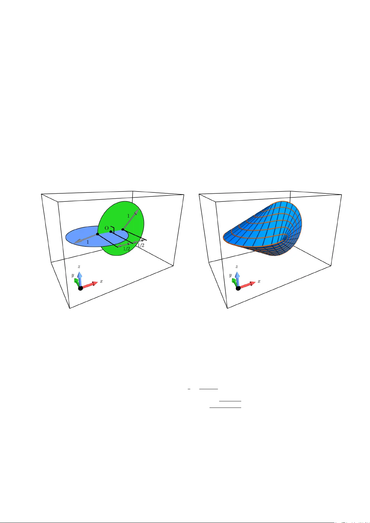
The momen t of inertia tensor of an oloid Sander G. Huisman Physics of Fluids Dep artment, Max Planck Center for Complex Fluid Dynamics, and J. M. Burgers Centr e for Fluid Dynamics, University of Twente, P.O. Box 217, 7500AE Ensche de, The Netherlands (Dated: Marc h 17, 2026) The oloid is defined as the con vex hull of tw o unit circles in p erp endicular planes, each passing through the center of the other. In this paper we deriv e an analytical expression for the moment of inertia tensor of an oloid with uniform density and confirm the result numerically . I. INTR ODUCTION The oloid w as introduced by P aul Sc hatz in 1929. It is obtained as the conv ex h ull of t wo unit circles in perp endicular planes, where each circle passes through the center of the other. The underlying construction and the resulting geometry are shown in Fig. 1. The oloid is a developable roller, sp ecifically , it is part of the family of so-called t wo-circle rollers, and it is also closely related to the sphericon, p olycons, and platonicons. These t yp es of particles ha ve even b een customized to follo w a specific path [1]. The oloid has also b een used in the field of fluid mechanics to study the settling of such a particle inside a fluid [2]. FIG. 1: Left: Geometry of the tw o intersecting circles, here shown as colored disk. The tw o unit circles lie in p erp endicular planes and their cen ters are lo cated at a distance 1 / 2 from the origin O. Right: Conv ex hull of the configuration on the left, with an added mesh to visualize the 3D surface. The orange mesh-lines are for constant m and the blue mesh-lines are for constan t t . Both figures include the directions of the axes x , y , and z , see the gnomons in the b ottom left, the origin (O) is at the geometrical center of the shap e which coincides with the center of mass. W e place the origin (O) at the midp oint of the tw o centers, such that the centers are a distance 1 / 2 from the origin. The conv ex hull can then b e describ ed parametrically as [3]: P ( m, t ) =   x ( m, t ) y ( m, t ) z ( m, t )   =    − 1 2 + m cos( t )+1 + ( m − 1) cos( t ) (1 − m ) sin( t ) ± m √ 2 cos( t )+1 cos( t )+1    , (1) where 0 ≤ m ≤ 1 and − 2 π / 3 ≤ t ≤ 2 π / 3. Here the ± describ es the upp er and low er part of the hull; combining the t wo then gives the complete hull. Previously , it has b een shown that the area of the ob ject is A = 4 π [3]. That pap er also rep orted the numerical v alue of the volume. Here we express the result as the sum of tw o elliptic integrals (which 2 can b e found by sym b olically in tegrating their Eq. 32): V = 2 3 K  3 4  + 4 3 E  3 4  = 3 . 05241846842437 . . . (2) where K and E are the complete elliptic in tegral of the first kind and second kind, resp ectively: K ( m ) = π / 2 ˆ 0 1 p 1 − m sin( θ ) 2 d θ (3) E ( m ) = π / 2 ˆ 0 p 1 − m sin( θ ) 2 d θ . (4) Mo deling the rotational dynamics of an oloid requires the moment of inertia tensor, which is comp osed of 9 comp onents: I ij = ˆ ˆ ˆ V ρ ( x k x k δ ij − x i x j ) d V =   I xx I xy I xz I y x I y y I y z I z x I z y I z z   (5) where w e used the Einstein summation conv ention, and we will assume ρ = 1 from now on (uniform unit density). W e know that the tensor is symmetric, such that w e are lo oking for (at most) 6 unique elemen ts (3 diagonal, 3 off-diagonal). W e choose our axes as in figure 1, the origin (O) is aligned with the cen ter of mass. The axis defined b y the intersection of the tw o symmetry planes of the oloid (the x direction through the origin O) is a principal axis. The remaining tw o axes can be chosen freely (provided they are mutually p erp endicular and p erp endicular to the first axis). F or conv enience we align them with the planes of the circles. By choosing the principal axes the moment of inertia tensor is simplified and all the off-diagonal terms are zero: I ij =   I xx 0 0 0 I y y 0 0 0 I z z   . (6) Alternativ ely , one can see from the definition of the moment of inertia (for uniform unit densit y): I xy = ˆ ˆ ˆ V xy d V (7) that b ecause the b o dy is symmetric with resp ect to y → − y , this transformation implies: I xy = − I xy (8) from which we conclude that the v alue m ust b e 0. W e can do this also for the I y z term, as w ell as for the I xz term (b ecause of the symmetry in the z plane), and b ecause the tensor is symmetric thus also for the I y x , I z y , and I z x terms. In addition, b ecause of the additional symmetry of the particle we see that I y y = I z z suc h that we are left to calculate tw o v alues: I xx = ˆ ˆ ˆ V  y 2 + z 2  d V (9) I y y = ˆ ˆ ˆ V  x 2 + z 2  d V . (10) T o ev aluate these in tegrals w e use the divergence theorem to conv ert the volume in tegral to a surface integral: I xx = ‹ S   x  y 2 + z 2  0 0   · d  S (11) I y y = ‹ S   0 y  x 2 + z 2  0   · d  S (12) 3 where S is the surface of V and d  S is the infinitesimal surface area m ultiplied by the local outw ard-facing normal v ector. Using the parametric representation of the surface, this b ecomes: I xx = ‹ S   x  y 2 + z 2  0 0   · d  S = 2 1 ˆ 0 2 π / 3 ˆ − 2 π / 3   x  y 2 + z 2  0 0   ·  d P d m × d P d t  d t d m (13) I y y = ‹ S   0 y  x 2 + z 2  0   · d  S = 2 1 ˆ 0 2 π / 3 ˆ − 2 π / 3   0 y  x 2 + z 2  0   ·  d P d m × d P d t  d t d m (14) where the factor of 2 accounts for the upp er and low er parts of the surface. W e now calculate the last brack eted term; the cross pro duct of the surface tangents (here we hav e take parameterisation of the top shell; the + version of the z comp onen t of Eq. 1): d P d m =      cos( t ) + 1 cos( t )+1 − sin( t ) √ 2 cos( t )+1 cos( t )+1      (15) d P d t =      sin( t )  m  1 (cos( t )+1) 2 − 1  + 1  (1 − m ) cos( t ) m sin( t ) cos( t ) (cos( t )+1) 2 √ 2 cos( t )+1      . (16) W e then hav e: d P d m × d P d t =      cos( t )((3 m − 2) cos( t ) − 1) 2 cos ( t 2 ) 2 √ 2 cos( t )+1 sin( t )((2 − 3 m ) cos( t )+1) (cos( t )+1) √ 2 cos( t )+1 (2 − 3 m ) cos( t )+1 cos( t )+1      . (17) W e now hav e all the ingredients to ev aluate the integrals of Eqs. 13 and 14. Note that x , y , and z are defined in terms of m and t , see Eq. 1. After substituting everything we obtain: I xx = 1 ˆ 0 2 π/ 3 ˆ − 2 π/ 3 cos( t )((3 m − 2) cos( t ) − 1)  m cos( t )+1 + ( m − 1) cos( t ) − 1 2   m 2 (2 cos( t )+1) (cos( t )+1) 2 + ( m − 1) 2 sin( t ) 2  cos  t 2  2 p 2 cos( t ) + 1 d t d m (18) I yy = 1 ˆ 0 2 π/ 3 ˆ − 2 π/ 3 2(1 − m ) sin( t ) 2 ((2 − 3 m ) cos( t ) + 1)  ( m − 1) 2 cos( t ) 2 − ( m − 1) cos( t ) + m  2 m + 1 cos( t )+1 − 2  + 1 4  (cos( t ) + 1) p 2 cos( t ) + 1 d t d m. (19) The integration with resp ect to m is p olynomial of degree 4 and results in: I xx = 2 π/ 3 ˆ − 2 π/ 3 − cos( t ) 2 ( − 2510 cos( t ) + 547 cos(2 t ) + 1129 cos(3 t ) + 648 cos(4 t ) + 181 cos(5 t ) + 21 cos(6 t ) − 1744) 15360 cos  t 2  8 p 2 cos( t ) + 1 d t (20) I yy = 2 π/ 3 ˆ − 2 π/ 3 (542 cos( t ) + 322 cos(2 t ) + 122 cos(3 t ) + 21 cos(4 t ) + 361) tan  t 2  2 240 p 2 cos( t ) + 1 d t. (21) These expressions can b e integrated with resp ect to t manually or using a computer algebra system (CAS): I xx = 32 45 E  3 4  − 2 45 K  3 4  = 0 . 76535025749314262939 . . . (22) I y y = I z z = 71 45 E  3 4  − 19 90 K  3 4  = 1 . 45551287346920034498 . . . (23) 4 T o calculate these constants precisely one can use the link b etw een elliptic integrals and Gauss’s arithmetic-geometric mean (AGM) to develop an algorithm that conv erges quadratically . W e hav e confirmed the v alue of these num b ers b y numerically in tegrating Eqs. 18 and 19. In addition, a Monte Carlo sim ulation in which 10 6 random p oints are generated inside the hull and calculating the moment of inertia also confirms these num b ers up to 2 decimal places. F or an oloid constructed from circles with a radius r and unit density the momen t of inertia is given by: I ( r ) =     I xx 0 0 0 I y y 0 0 0 I z z     r 5 . (24) Ac knowledgmen ts W e thank Mees Flapper, Detlef Lohse, Bernhard Mehlig, John Sader, F ederico T oschi, Leen v an Wijngaarden, Xander de Wit, and Greg V oth for stimulating discussions ab out the oloid. [1] Y. I. Sob olev, R. Dong, T. Tlusty , J.-P . Eckmann, S. Granick, and B. A. Grzyb owski, Nature 620 , 310 (2023). [2] M. M. Flapp er, G. Piumini, R. V erzicco, S. G. Huisman, and D. Lohse, arXiv preprint arXiv:2511.05137 (2025). [3] H. Dirnb¨ oc k and H. Stachel, J. Geom. Graph 1 , 105 (1997). App endix: Area calculation Finding the area of the oloid can b e found by integrating the magnitude of the normal v ector from Eq. 17: A = 2 1 ˆ 0 2 π / 3 ˆ − 2 π / 3         d P d m × d P d t         d t d m (25) A = 1 ˆ 0 2 π / 3 ˆ − 2 π / 3 (4 − 6 m ) cos( t ) + 1 cos  t 2  p 2 cos( t ) + 1 d t d m (26) A = 2 π / 3 ˆ − 2 π / 3 cos( t ) + 2 cos  t 2  p 2 cos( t ) + 1 d t (27) A = 4 π (28) confirming the results of Ref. [3].