Timely Best Arm Identification in Restless Shared Networks

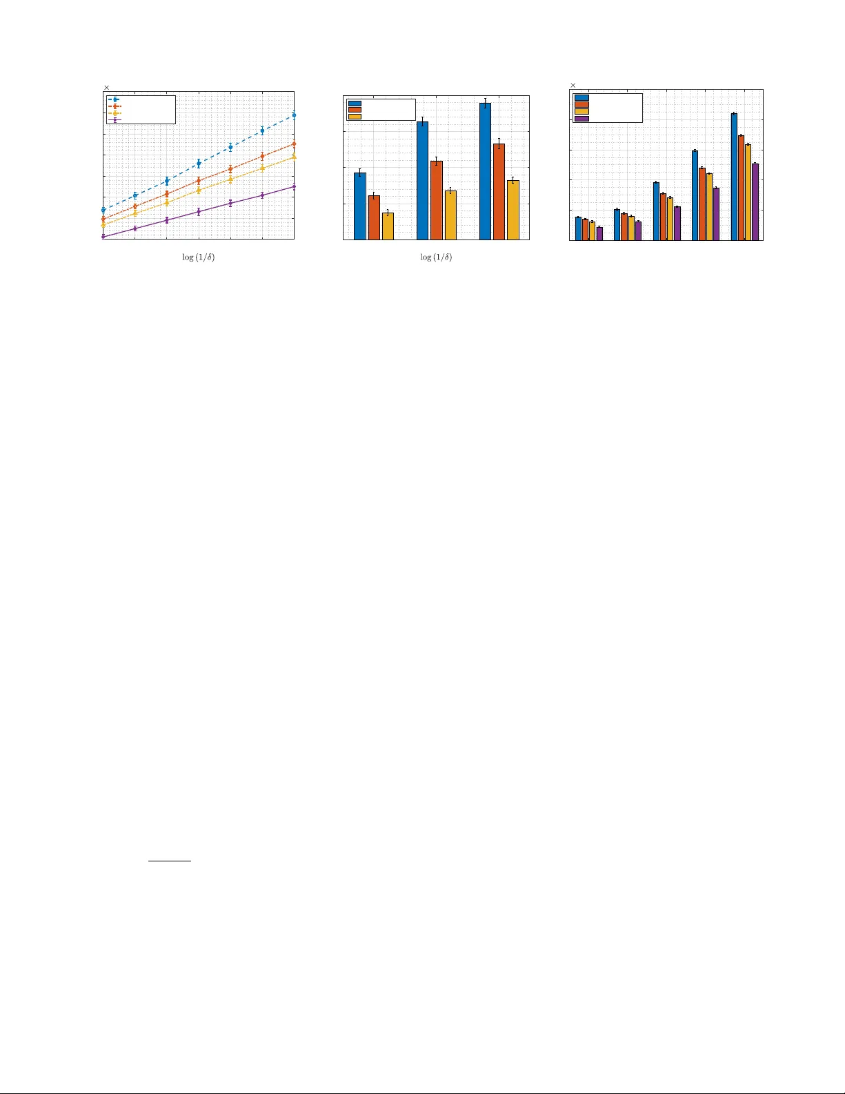
JOURNAL OF L A T E X CLASS FILES, VOL. 14, NO. 8, A UGUST 2021 1 T imely Best Arm Identification in Restless Shared Networks Mengqiu Zhou, Student Member , IEEE, V incent Y . F . T an, Senior Member , IEEE, and Meng Zhang, Member , IEEE Abstract —Real-time status updating applications increasingly rely on networks of devices and edge nodes to maintain data freshness, as quantified by the age of inf ormation (AoI) metric. Given that edge computing nodes exhibit uncertain and time- varying dynamics, it is essential to identify the optimal edge node with high confidence and sample efficiency , even without prior knowledge of these dynamics, to ensure timely updates. T o address this challenge, we intr oduce the first best arm identification (B AI) problem aimed at minimizing the long-term av erage AoI under a fixed confidence setting, framed within the context of a restless multi-armed bandit (RMAB) model. In this model, each arm ev olves independently according to an unknown Markov chain over time, regardless of whether it is selected. T o capture the temporal trajectories of AoI in the presence of unknown restless dynamics, we develop an age-aware LUCB algorithm that incorporates Markovian sampling. Additionally , we establish an instance-dependent upper bound on the sample complexity , which captures the difficulty of the problem as a function of the underlying Markov mixing behavior . Moreo ver , we derive an information-theoretic lower bound to characterize the fundamental challenges of the problem. W e show that the sample complexity is influenced by the temporal corr elation of the Marko v dynamics, aligning with the intuition offered by the upper bound. Our numerical results show that, compared to existing benchmarks, the proposed scheme significantly reduces sampling costs, particularly under more stringent confidence levels. Index T erms —age of inf ormation, restless multi-armed bandit, best arm identification I . I N T R O D U C T I O N A. Backgr ound and Motivations Information freshness is becoming increasingly significant due to the rapid growth of real-time applications. For in- stance, in vehicular networks, timely status updates regarding traffic conditions and vehicle status are vital for reliable autonomous driving [1]. Similarly , industrial control systems depend on immediate alerts of equipment anomalies, such as overheating and abnormal pressure lev els, to maintain operational safety [2]. In addition, real-time health monitoring updates from wearable devices enables prompt medical inter- ventions [3]. T o quantify data freshness, the age of information (AoI) metric has been introduced [4], which measures the time that has elapsed since the most recent data update. Mengqiu Zhou is with the College of Information Science and Electronic Engineering and ZJU-UIUC Institute, Zhejiang Univ ersity , China (e-mail: mengqiuzhou@zju.edu.cn). V incent Y . F . T an is with the Department of Mathematics, the Department of Electrical and Computer Engineering, and the Institute of Operations Research and Analytics, National Univ ersity of Singapore (e-mail: vtan@nus.edu.sg). Meng Zhang is with the ZJU-UIUC Institute, Zhejiang University , China (e-mail: mengzhang@intl.zju.edu.cn). Fresh data deli very in such applications critically relies on Mobile Edge Computing (MEC) infrastructures [5], where computational tasks are offloaded to edge nodes such as base stations or roadside units located at the network edge. A fundamental challenge in public edge networks lies in the uncertainty of shared resources. Unlike priv ate servers, edge nodes operate as shared infrastructure serving a large number of background users. In practice, users are typically served through virtualized compute slices with standardized resource specifications at each edge node, while performance variability primarily arises from time-varying background workloads. From the perspecti ve of a specific user (e.g., a connected vehicle), the internal congestion state of an edge node is unobservable and ev olves continuously o ver time, regardless of whether the user selects it. As a result, a node that deliv ered fresh updates moments ago may become heavily congested due to sudden bursts of background traffic. This creates a r estless en vironment in which the user must repeatedly decide which edge node to query without direct kno wledge of its instantaneous load. Extensiv e research has inv estigated AoI optimization focus- ing on task offloading strategy [6], [7], transmission schedul- ing [8]–[10] and resource allocation mechanism [11]–[13]. Regrettably , all of these ef forts rely on prior knowledge of system dynamics. In particular , while recent pioneering studies hav e formulated AoI minimization problems within the restless multi-armed bandit (RMAB) framework and designed index-based scheduling policies [9], [13], they assume known transition probabilities to enable tractable solutions such as Whittle’ s index [14]. In practical open edge networks, continuously learning or tracking the complete, time-varying transition models of all edge nodes is often computationally prohibitive and resource- intensiv e, as such information is typically hidden from indi- vidual users. Moreo ver , although dynamic scheduling could theoretically exploit instantaneous idle slots, it is frequently impractical in stateful edge applications due to prohibitiv e switching overheads, including context migration and connec- tion re-establishment costs. Therefore, the crucial requirement in practice is to quickly and reliably identify a stable and high-performing edge node that ensures data freshness under unknown system dynamics, rather than continuously switching among nodes. This motiv ates our ke y question: Key Question. How should one design a sample-efficient age- optimal best edge node identification strate gy under unknown and time-varying dynamics? JOURNAL OF L A T E X CLASS FILES, VOL. 14, NO. 8, A UGUST 2021 2 T o address the unobservability of network state, we model the internal dynamics of each edge node using a Hidden Markov Model (HMM), where the hidden state represents a congestion level induced by background traffic. Unlike classical queueing models that assume observable queue lengths [15], our abstraction captures the limited visibility faced by users in realistic edge networks. W e formulate this problem as an age-optimal Best Arm Identification (B AI) task under a fixed-confidence setting within the RMAB framework, aiming to identify the edge node that minimizes the long-term av erage AoI with minimal sampling cost. Solving this problem is particularly challenging due to the presence of unknown restless dynamics and temporal cor- relations in observations. Classical concentration inequalities designed for i.i.d. samples (e.g., Chernoff [16] or Hoeffding [17] bounds) are no longer applicable, and the autonomous ev olution of unselected nodes further complicates learning under partial observations. B. Contributions Our key contributions are summarized as follows. • Pr oblem F ormulation : W e propose a novel age-optimal best arm identification problem in the restless multi-armed bandit framew ork under a fixed-confidence setting. T o the best of our knowledge, this is the first work to identify edge node performance under unknown and restless dynamics, with the objectiv e of minimizing the av erage age of information. • Age-Optimal Best Arm Identification : T o overcome the non- con ve xity of our age-optimal BAI problem which has a frac- tional cost, we transform it into an equiv alent average cost problem. T o handle the partial observ ability in RMAB, we dev elop an age-awar e LUCB algorithm which incorporates a Markovian sampling strategy . Further , we establish an instance-dependent upper bound on the sample complexity and sho w that the bound depends on the mixing behavior of underlying Markovian dynamics. • Lower Bound: W e deri ve a family of information-theoretic lower bounds on the sample complexity parameterized by a certain quantity known as the delay constraint D . W e con- duct a case study for a two-arm, two-state case with D = 2 . This study re veals that the fundamental sample comple xity is critically shaped by the temporal correlation of the Marko v dynamics, consistent with the mixing dependence observed in the upper bound analysis. • Numerical Results : W e compare the age-optimal B AI scheme to three benchmarks in terms of sample complexity . Numerical results show that our scheme can reduce the sample complexity by up to 43% relativ e to the benchmarks, with greater savings achiev ed under stricter confidence re- quirements. Moreover , the sample complexity gains become increasingly pronounced for harder instances characterized by smaller AoI gaps. I I . R E L AT E D W O R K In this section, we briefly revie w the literature related to our proposed age-optimal B AI. Related works can be classified into two categories: AoI and RMAB. A. Age of Information AoI, which measures the freshness of status update, has motiv ated extensi ve research since its introduction in [18]. Existing works along this line mainly focus on minimizing time-av erage AoI under a variety of system settings, including queueing networks (e.g., [11], [19]–[21]), computing systems (e.g., [22], [23]) and wireless networks (e.g., [24]–[26]). Some pioneering works have recently adopted the restless multi-armed bandit (RMAB) framework to address AoI-aware source scheduling problems [9], [13], [27], in which Whit- tle’ s inde x is used to design lo w-complexity policies. These approaches typically assume full knowledge of the underlying Markov transition model and rely on structural properties such as indexability to derive closed-form indices. However , none of these works consider the age minimization problem under unknown system dynamics due to the unobservable conges- tion status, wher e such index-based methods are not directly applicable. T o fill this gap, we study the best edge node identification problem under unknown Markovian dynamics, aiming to minimize the av erage AoI in this paper . B. Restless Multi-Armed Bandit The RMAB generalizes the classical bandit by allowing each arm to ev olve continuously ov er time, regardless of selection. Since its introduction by Whittle in [14], the RMAB has been extensi vely studied due to its modeling flexibility and analytical challenges. Prior research on RMAB problems primarily focused on minimizing cumulati ve regret ov er a fix ed horizon, has explored a variety of solution approaches, in- cluding index-based heuristic policies (e.g., [28]–[30]), regret- based online learning approaches (e.g., [31]–[34]), and rein- forcement learning (e.g., [35], [36]). Howe ver , in mission- critical applications (e.g., autonomous driving) where data stal- eness can compromise safety , cumulative regret minimization is often insufficient. In such scenarios, the BAI problem which aims to identify the best arm with high confidence using as few samples as possible is more suitable, yet receiv es limited attention in the RMAB context. T o the best of our kno wledge, only [37] has addressed this issue. Nevertheless, all of these efforts define the best arm as the one with the highest expected r ewar d, without considering structur ed objectives such as Age of Information, which poses unique challenges as it r equir es trac king over temporal trajectories rather than instantaneous r ewar ds. I I I . S Y S T E M M O D E L In this section, we consider a status update system illustrated in Fig. 1, consisting of a source, a scheduler, K edge nodes with unknown congestion dynamics induced by background traffic, and a monitor . The scheduler submits update packets to one of the edge nodes, each of which operates under a first-come-first-served (FCFS) discipline and is subject to additional, unobservable workloads generated by other users. W e no w start with models for the restless edge node model and the time-average age metric in order to then formulate the age-optimal best arm identification problem via restless multi- armed bandit framework. For any positiv e integer A , we use [ A ] ≜ { 1 , 2 , . . . , A } to denote the set of integers up to A . JOURNAL OF L A T E X CLASS FILES, VOL. 14, NO. 8, A UGUST 2021 3 Source Scheduler Updates Backgroun d T raff ic Edge Nodes Monit or …… Node 1 Node 𝐾 Node 2 Fig. 1. The system model. Each edge node is modeled as an arm in a restless multi-armed bandit framework, with unknown congestion dynamics. A. Restless Edge Node Model W e consider a cluster of K edge nodes, each of which is shared by multiple services and is responsible for processing update packets from external sources in the network. Suppose the i th update packet is submitted to edge node a ∈ [ K ] . At that instant, the node is characterized by a congestion state X a,i ∈ S = { 0 , 1 , . . . , S } , which represents the background workload and contention effects induced by other users in the network. W e model the background traf fic dynamics of each node as a stationary ergodic Markov chain with unknown transition probability denoted by P a ( s ′ | s ) = Pr[ X a,i +1 = s ′ | X a,i = s ] . Due to the lack of visibility into the internal congestion lev els in practice, the scheduler does not observe X a,i directly and instead observes the service delay Y a,i ∈ Y upon completion of update i processed by edge node a . As a result, the pair ( X a,i , Y a,i ) forms a Hidden Markov Model (HMM), where the emission probability is defined as Pr [ Y a,i = y | X a,i = s ] . Motiv ated by network slicing techniques [38], [39] widely applied in practical mobile edge computing systems, the user is served by a standardized compute slice (e.g., a container with fixed CPU/bandwidth quotas) at each node. In such virtualized en vironments, the service delay experienced by the user is primarily gov erned by background congestion. Accordingly , we start with adopting a deterministic emission model as a first-order approximation, where Pr[ Y a,i = y | X a,i = s ] = 1 and the observation space is Y = { f (0) , f (1) , . . . , f ( S ) } . The congestion state X a,i is driv en by exogenous back- ground traf fic. In a spatially distrib uted edge network, traf- fic patterns across different locations (e.g., business districts versus residential areas) are typically weakly correlated. W e therefore assume that the state transitions of different edge nodes are independent. Under this setting, the transition prob- ability of each arm varies primarily in its background arri val characteristics, which are commonly modeled as Poisson pro- cesses. T o capture a broad class of transition behaviors while retaining analytical tractability , we assume that each node’ s transition probability matrix is generated from a one-parameter exponential family studied in [40]. W e introduce a real-valued parameter θ a ∈ R to charac- terize the transition dynamics of each arm a and denote its transition probability matrix by P θ a . Specifically , we fix an irreducible base transition matrix P ov er S and construct the unnormalized matrix for any edge node a given as ˜ P θ a ( s ′ | s ) ≜ P ( s ′ | s ) exp( θ a · f ( s ′ )) , ∀ s, s ′ ∈ S . (1) W e denote the full collection of arm-specific parameters by θ ≜ [ θ 1 , . . . , θ K ] ⊤ and refer to θ as the problem instance. Note that ˜ P θ a defined in (1) is not a v alid stochastic transition probability matrix as its rows do not necessarily sum up to one. T o address this, we normalize (1) by in voking Perron-Frobenius theory . For each θ a , let ρ ( θ a ) denote the Per - ron–Frobenius eigen value of ˜ P θ a and v θ a = [ v θ a ( s ) : s ∈ S ] ⊤ be its corresponding unique positive right eigen vector [41, Theorem 8.4.4]. The normalized transition probability matrix P θ a is specified by P θ a ( s ′ | s ) = v θ a ( s ′ ) ρ ( θ a ) v θ a ( s ) ˜ P θ a ( s ′ | s ) , s, s ′ ∈ S . (2) T o ensure that each P θ a defines as an ergodic Markov chain, we begin by defining ¯ f = max s f ( s ) and f = min s f ( s ) , and the associated lev el sets S ¯ f = { s ∈ S : f ( s ) = ¯ f } and S f = { s ∈ S : f ( s ) = f } . W e then impose the follo wing mild conditions on the stochastic matrix P . Assumption 1. W e assume that the matrix P satisfies: A1: The submatrix of P with r ows and columns in S ¯ f is irr educible. A2: F or every s ∈ S \ S ¯ f , ther e exists s ′ ∈ S ¯ f such that P ( s ′ | s ) > 0 . A3: The submatrix of P with r ows and columns in S f r epr e- sents an irr educible Markov chain. A4: F or every s ∈ S \ S f , ther e exists s ′ ∈ S f such that P ( s ′ | s ) > 0 . Assumption 1 accommodates a wide range of models as it only requires partial irreducibility and accessibility to ir- reducible subsets. In particular , any transition matrix P with strictly positiv e entries trivially satisfies the above conditions. Based on [42], we establish the following lemma. Lemma 1. When P repr esent an irreducible transition pr ob- ability matrix on the finite state space S satisfying Assump- tion 1, for any θ a , the matrix P θ a is irreducible and positive r ecurr ent. Lemma 1 implies that P θ a has a unique stationary distribu- tion, which we denote by µ θ a = [ µ θ a ( s ) : s ∈ S ] ⊤ . Since the underlying congestion state of each node continues to ev olve ev en when not selected, we adopt a RMAB framework by modeling each node as an independent arm whose state ev olves over a finite state space S according to a discrete- time, time-homogeneous Markov process. B. T ime-A verage Age An age of information (AoI) metric is used to characterize timeliness by the v ector of ages tracked by monitors [4]. As JOURNAL OF L A T E X CLASS FILES, VOL. 14, NO. 8, A UGUST 2021 4 𝑌 ! 𝑌 !" # 𝑌 $ 𝑌 % 𝑌 $ 𝑡 ! 𝑡 ! & (𝑡 !" # ) 𝑡 !" # & 𝑡 𝑌 # 𝑡 $ & (𝑡 % ) 𝑡 % & 𝑡 $ 𝑄 ! 𝑌 !" # 𝑌 % Δ 𝑡 𝑌 ! Fig. 2. Age of information ∆( t ) ev olution in time under zero-wait policy . depicted in Fig. 1, the updating system has a source that sub- mits updates with computational requirements to a scheduler, which selects one of the K edge nodes for processing before deliv ering those updates to a destination monitor . Suppose the source observes an acknowledgement from the monitor and generate fresh updates as a stochastic process at times { t i : i ∈ N } , with each update time-stamped t i . W e first consider the zero-waiting policy . 1 These updates are processed by the node and deliv ered to the destination monitor at times { t ′ i : i ∈ N } . This induces the AoI process ∆( t ) has a characteristic sawtooth shape depicted in Fig. 2. Denote the service time for update i as Y i , the AoI process ∆( t ) at the destination monitor is reset at time t ′ i to ∆( t ′ i ) = Y i , the age of the update receiv ed at that time instant. AoI analysis was initiated in [18], which defines the time- av erage AoI as ∆ ( ave ) = lim T →∞ 1 T Z T 0 ∆( t ) dt. (3) This time-average was ev aluated by graphically decomposing the integral into areas Q i , as shown in Fig. 2. Follo wing this approach, we define epoch i as the time interval [ t i , t ′ i ) and we observe from Fig. 2 that associated with this epoch is the area Q i = Q ( Y i , Y i +1 ) ≜ 1 2 ( Y i + Y i +1 ) 2 − 1 2 Y 2 i +1 = 1 2 Y 2 i + Y i Y i +1 . (4) It follows that the long-term average AoI is thus gi ven by [4]: ∆ ( ave ) ≜ lim sup n →∞ P n i =1 E [ Q ( Y i , Y i +1 )] P n i =1 E [ Y i ] . (5) C. Pr oblem F ormulation Our goal is to minimize the long-term a verage AoI ∆ (av e) by selecting the best node a ∈ [ K ] with high confidence and minimal samples. W e use Y a,i to denote the service time experienced by the i th packet processed by node a ∈ [ K ] , then the problem can be formulated as min a ∈ [ K ] lim sup n →∞ P n i =1 E [ Q ( Y a,i , Y a,i +1 )] P n i =1 E [ Y a,i ] . (6) 1 Optimizing the w aiting strategy in age-optimal B AI problem will be further in vestigated in our future work. It follows from Lemma 1 that each node a is associated with a Markov chain with a unique stationary distribution. Hence, we drop the index n and Problem (6) can be simplified as γ ∗ ≜ min a ∈ [ K ] E [ Q ( Y a,i , Y a,i +1 )] E [ Y a,i ] . (7) In order to overcome the noncon ve xity of the objecti ve E [ Q ( Y a,i , Y a,i +1 )] / E [ Y a,i ] , we use the fractional programming technique by optimizing the expected value of the dif ference D ( Y a,i , Y a,i +1 , γ ) ≜ Q ( Y a,i , Y a,i +1 ) − γ Y a,i , (8) where γ is the Dinkelbach variable [43]. With this definition, the Dinkelbach reformulation is J ( γ ) = min a ∈ [ K ] E [ D ( Y a,i , Y a,i +1 , γ )] . (9) Giv en the optimal node a ∗ to Problem (7), we have E [ D ( Y a,i , Y a,i +1 , γ ∗ )] ≥ 0 and E [ D ( Y a ∗ ,i , Y a ∗ ,i +1 , γ ∗ )] = 0 , indicating that a ∗ is also optimal to Problem (9). This estab- lishes the equi valence of Dinkelbach’ s transformation in the stationary policy space. The following lemma [43, Theorem 1] guarantees the equiv alence of the transformed problem. Lemma 2. [43, Theor em 1] When γ ∗ is the optimum objective value of Pr oblem (7) , Pr oblem (9) with γ = γ ∗ is equivalent to Pr oblem (7) and J ( γ ∗ ) = 0 . Lemma 2 shows the possibility of equi valently reformulat- ing the fractional objectiv e into one with an av erage cost. In addition, the Dinkelbach’ s method suggests that the optimum objectiv e γ ∗ of Problem (7) satisfies J ( γ ∗ ) = 0 and hence conducting a line search over γ leads to the optimal arm a ∗ . W e note that the av erage-cost objecti ve is essential for the best arm online learning that will be discussed in Section V. Unlike traditional MAB formulations that rely on immediate rew ards, our objectiv e is tightly coupled with the underlying Markovian state transitions. This dependency requires rea- soning over long-term temporal trajectories under unknown node dynamics rather than single-step outcomes, which is significantly more challenging as it deviates from standard bandit assumptions and makes sampling strategies based on instantaneous rew ards inapplicable. I V . B E S T A R M I D E N T I FI C A T I O N T o identify the best node a ∈ [ K ] that minimizes the long- term average AoI ∆ ( ave ) with high confidence and sample efficienc y , we formulate our problem as a BAI task under the fixed-confidence setting. A. Definition of Age-Optimal Best Arm Follo wing with the restless edge node model in Section III-A, giv en the stationary distribution µ θ a of arm a , Problem (9) is equiv alent to min a ∈ [ K ] X s ∈S µ θ a ( s ) h 1 2 f 2 ( s ) − γ f ( s ) i + X s,s ′ ∈S µ θ a ( s ) P θ a ( s ′ | s ) f ( s ) f ( s ′ ) . (10) JOURNAL OF L A T E X CLASS FILES, VOL. 14, NO. 8, A UGUST 2021 5 T o facilitate analysis, we decompose the objective in (10) into a transition-independent term η θ a ( γ ) and transition-dependent term Γ θ a , giv en as η θ a ( γ ) ≜ X s ∈S  1 2 f 2 ( s ) − γ f ( s )  µ θ a ( s ) , a ∈ [ K ] , (11) Γ θ a ≜ X s ∈S f ( s ) f ( s ′ ) P θ a ( s ′ | s ) µ θ a ( s ) , a ∈ [ K ] . (12) Therefore, Problem (10) reduces to min a ∈ [ K ] g θ a ( γ ) ≜ η θ a ( γ ) + Γ θ a . (13) Giv en the Dink elbach variable γ , we define the age-optimal best arm a ∗ ( θ , γ ) under instance θ ≜ [ θ 1 , . . . , θ K ] ⊤ as a ∗ ( θ , γ ) ≜ argmin a ∈ [ K ] g θ a ( γ ) . (14) Our goal is to identify a ∗ ( θ , γ ) in a sample-efficient manner without any prior knowledge of the instance θ . W e formulate this B AI problem under a fixed-confidence setting, where the scheduler aims to identify the best arm with as few samples as possible while ensuring that the misidentification probability is limited to a pre-specified confidence lev el. B. Best Arm Identification P olicy T o identify the best arm, the scheduler sequentially selects edge nodes to process update packets and observes the re- sulting service times. Let A n ∈ [ K ] denote the arm selected for the n th update and let Y n be the corresponding observed service time. Note that we adopt the restless bandit setting, in which each arm e volves according to its internal Markovian dynamics, regardless of whether it is selected. Let F n be the σ -field generated by the sequence of past actions and observations up to update n , i.e., F n ≜ σ ( A 1 , Y 1 , . . . , A n , Y n ) . (15) A B AI policy under the fix ed-confidence setting consists of: • Sampling rule π = { π n } n ≥ 1 : an F n − 1 -measurable rule that determines the arm A n to be selected for update n ; • Stopping rule τ : a stopping index adapts {F n : n ≥ 1 } indicating when to terminate the arm selection process; • Decision rule a τ : an F τ -measurable rule that specifies the candidate best arm a ∈ [ K ] at termination. Giv en a confidence lev el δ ∈ (0 , 1) , we define Π( δ ) ≜ ( ( π , τ , a τ ) : P θ ( a τ  = a ∗ ( θ , γ )) ≤ δ P θ ( τ < ∞ ) = 1 ) (16) as the set of all policies that terminate in finite time with probability one and upon termination outputs the best arm with probability at least 1 − δ . Our objectiv e is to design a policy π ∈ Π( δ ) that minimizes the expected sample complexity for solving Problem (14), which is equi valent to characterize the value of inf π ∈ Π( δ ) E θ [ τ π ] . (17) W e consider the regime in which δ → 0 . Howe ver , the struc- tural complexity of our AoI minimization problem originating …… …… ! 𝑌 ! ! 𝑌 ! …… ! 𝑌 !" ! 𝑌 !" …… B lock 1 , pull arm 𝑎 B lock 2 , pull arm 𝑎′ Step 1 Step 2 Step 3 Step 1 Step 2 Step 3 …… …… ! 𝑌 !"" …… B lock b n , pull arm 𝑎′′ update 𝑛 update T(𝑛) ! 𝑌 !"" Fig. 3. The structure of the Markov regeneration sampling strategy . from its dependence on long-term Markovian dynamics poses significant challenges for efficient algorithm design, as we discuss in the following section. V . A G E - O P T I M A L B A I A L G O R I T H M W e now describe the key ideas of our proposed age-optimal B AI algorithm which is a policy satisfying (16). The global structure of the age-optimal BAI algorithm consists of three loops, including Marko v Regeneration Sampling, Age-A ware LUCB procedure and Dinkelbach Update. A. Markov Re generation Sampling Strate gy It follo ws from (13) that our objectiv e includes a transition- dependent term Γ θ a , which requires tracking long-term tem- poral trajectories governed by unknown node congestion tran- sitions. T o address this temporal dependence between consec- utiv e samples, we propose a Marko v regeneration sampling strategy inspired based on the regenerati ve process introduced in [44]. Since we consider the deterministic emission setting, for each arm a , we define a regenerati ve state ˜ X a with associated observation ˜ Y a , which marks both the beginning and end of a Markov regeneration process. W e define b ( n ) as the number of completed blocks up to update n , and T ( n ) as the update index marking the end of the most recently completed block. As depicted in Fig. 3, each sampling block b ∈ { 1 , 2 , . . . } consists of the following steps: • Initialization (Step 1) : Pull arm a repeatedly until the regenerati ve observation ˜ Y a is encountered; • Re generation Sampling (Step 2) : Continue sampling arm a and collecting observations until revisiting ˜ Y a ; • Block T ermination (Step 3) : Close the block upon the second observation of ˜ Y a . W e focus on the samples collected during the Markov re- generation process ( Step 2 ) of each block. Let j b denote the cumulativ e number of samples obtained in Step 2 across the first b blocks, and T a j b represent the total number of such samples collected from arm a . The corresponding observations JOURNAL OF L A T E X CLASS FILES, VOL. 14, NO. 8, A UGUST 2021 6 Algorithm 1: Markov Regeneration Sampling Input: Dinkelbach’ s variable γ , block index b , Step 2 update index j ; 1 Giv en counters and estimators for arm a : T a j , ˆ η a ( γ ) and ˆ Γ a based on (18a), (18b); // Step 1: Initialization 2 Play arm a and observe Y a ; 3 while Y a  = ˜ Y a do 4 i ← i + 1 ; 5 Play arm a and observe Y a ; // Step 2: Regeneration sampling 6 ˆ η a ( γ ) ← ˆ η a ( γ ) T a j +( 1 2 ˜ Y 2 a − γ ˜ Y a ) T a j +1 , ˆ Γ a ← ˆ Γ a T a j +0 T a j ; 7 i ← i + 1 , j ← j + 1 , T a j ← T a j + 1 ; 8 Set Y p = ˜ Y a ; 9 Play arm a and observe Y a ; 10 while Y a  = ˜ Y a do 11 ˆ η a ( γ ) ← ˆ η a ( γ ) T a j +( 1 2 Y 2 a − γ Y a ) T a j +1 , ˆ Γ a ← ˆ Γ a ( T a j − 1)+ Y p Y a T a j ; 12 i ← i + 1 , j ← j + 1 , T a j ← T a j + 1 ; 13 Set Y p ← Y a ; 14 Play arm a and observe Y a ; // Step 3: Block termination 15 ˆ Γ a ← ˆ Γ a ( T a j − 1)+ Y p ˜ Y a T a j ; 16 b ← b + 1 , i ← i + 1 ; are denoted by Y a, 1 , Y a, 2 , . . . , Y a,T a j b , from which we construct the empirical estimators: ˆ η a,T a j b ( γ ) = 1 T a j b T a j b X i =1  1 2 Y 2 a,i − γ Y a,i  , (18a) ˆ Γ a,T a j b = 1 T a j b T a j b X i =1 ( Y a,i Y a,i +1 ) . (18b) Hence, the empirical cost ˆ g θ a ( γ ) of arm a is giv en by ˆ g θ a ( γ ) = ˆ η a,T a j b ( γ ) + ˆ Γ a,T a j b . (19) T o bootstrap the regeneration process, the first block for each arm skips Step 1 by treating the initial observ ation as the regenerati ve point. The overall procedure for ex ecuting Markov regeneration sampling and updating the empirical estimators is summarized in Algorithm 1. B. Age-A ware LUCB algorithm Based on the Marko v regeneration sampling strategy , we now present the age-aware LUCB algorithm for identifying the age-optimal best arm with high confidence and sample efficienc y . A critical component in LUCB-type algorithms is the design of tight concentration bounds on the estimation, which support reliable confidence interv als that guide arm selection, comparison and stopping rules. Unlike classical bandit settings with i.i.d. observations, our restless Markovian model inv olves arms whose underlying states evolv e according to unknown and potentially non- rev ersible Markov chains. This presents a fundamental chal- lenge since standard concentration inequalities [16], [17] are no longer applicable due to the temporal correlations in the observations. T o obtain tight concentration bounds under Markovian de- pendence, it is essential to account for the mixing behavior of the chain, which captures the con ver gence rate to the stationary distribution. T o this end, we adopt the notion of the pseudo spectral gap [45], which extends spectral analysis to non- rev ersible Markov chains. Definition 1 (Pseudo Spectral Gap) . Given the transition pr obability matrix P θ a of arm a with stationary distrib ution µ θ a , let P ′ θ a denote its adjoint operator with r espect to the inner pr oduct on the Hilbert space L 2 ( µ θ a ) . Then, the pseudo spectral gap of arm a is defined as β θ a = max k ≥ 1 { β ′ (( P ′ θ a ) k P k θ a ) /k } , (20) wher e β ′ ( · ) denotes the spectral gap as defined in [46]. T o establish uniform concentration guarantees across all K arms, we introduce the global pseudo spectral gap β min ≜ min a ∈ [ K ] β θ a , which characterizes the worst-case mixing rate among all Markovian arms under the restless bandit setting. For quantifying initialization bias, we let q θ a denote the initial distribution of arm a and define the vector ω a ≜ ( q θ a ( s ) µ θ a ( s ) , s ∈ S ) to measure its de viation from stationarity . Using the Minko wski inequality and using a global lower bound on the stationary probabilities µ min = min a ∈ [ K ] min s ∈S µ θ a ( s ) , we bound the deviation as    ω a    2 ≤ X s ∈S    q θ a ( s ) µ θ a ( s )    ≤ 1 µ min . (21) Assuming µ min ≥ ¯ µ for some constant ¯ µ > 0 , we provide a uniform bound on initialization error , which enables us to state the following concentration bound motiv ated by [47, Theorem 3.3]. Proposition 1. Given a constant c ≥ 96( ¯ f 2 − f 2 ) 2 /β min and K arms, for any 0 < δ ≤ 1 , it holds that P " | ˆ g θ a ( γ ) − g θ a ( γ ) | < s c log (4 j b K/ ( δ ¯ µ )) T a j b # ≥ 1 − δ K . (22) Pr oof: See details in Appendix A. Follo wing the concentration bounds established in Propo- sition 1, we de velop the age-aw are LUCB selection scheme that integrates the Markovian regeneration sampling to enable reliable comparisons among arms with temporally correlated observations. Different from traditional LUCB methods that assume i.i.d. samples and update confidence interv als after each pull, our approach introduces a block-based update mechanism that ensures statistical validity under Markovian dynamics. Specif- ically , at each block index b , the algorithm computes the JOURNAL OF L A T E X CLASS FILES, VOL. 14, NO. 8, A UGUST 2021 7 Algorithm 2: Age-A ware LUCB Input: Dinkelbach’ s variable γ , confidence lev el δ ; 1 Initialize b = 1 , i = 0 , i 2 ( b ) = 0 , T a 2 ( i 2 ( b )) = 0 , ˆ η a = 0 , ˆ Γ a = 0 for all a ∈ [ K ] ; 2 for b ≤ K do 3 Play arm b and obtain ˆ η b b ( γ ) , ˆ Γ b b according to lines 6-16 of Algorithm 1; 4 while true do 5 for a = 1 , . . . , K do 6 Compute LCB a ( b ) according to (23a); 7 Set h ( b ) = argmin a ∈ [ K ] ˆ η b a ( γ ) + ˆ Γ b a ; 8 Set l ( b ) = argmin a  = h ( b ) LCB a ( b ) ; 9 Compute UCB h ( b ) according to (23b); 10 if UCB h ( b ) > LCB l ( b ) then 11 for a ′ ∈ { h ( b ) , l ( b ) } do 12 Play arm a ′ and obtain ˆ η b a ′ ( γ ) , ˆ Γ b a ′ according to Algorithm 1; 13 else 14 return a ∗ ( γ ) = h ( b ) empirical estimates ˆ η b a ( γ ) and ˆ Γ b a for each arm a and construct the lower and upper confidence bounds as follows: LCB a ( b ) = ˆ η b a ( γ ) + ˆ Γ b a − rad a ( b ) , (23a) UCB a ( b ) = ˆ η b a ( γ ) + ˆ Γ b a + rad a ( b ) , (23b) where rad a ( b ) is the confidence radius giv en as rad a ( b ) = s c log (4 j b K/ ( δ ¯ µ )) T a j b . (24) In each round b , as detailed in Lines 7 to 8 of Algorithm 2, the age-aware LUCB algorithm identifies two candidate arms: the current best arm h ( b ) , which minimizes the empirical cost estimate; and the challenger l ( b ) , which has the smallest lower confidence bound among the remaining arms. These two arms are selected for further exploration to reduce uncertainty and tighten the confidence intervals. The algorithm terminates when the upper confidence bound of the best arm falls below the lower confidence bound of its challenger , guaranteeing identification of the best arm with high confidence. C. Dinkelbach Update Lev eraging Lemma 2 and the monotonicity property that J ( γ ) decreases in γ , we adopt the bisection method to search for the optimal Dinkelbach variable γ ∗ such that J ( γ ∗ ) = 0 . Follo wing Problem (7), when the algorithm con verges, the minimum av erage age achiev ed by the best arm is γ ∗ . V I . U P P E R B O U N D O N T H E S A M P L E C O M P L E X I T Y In this section, we present an upper bound on the sample complexity of the proposed age-optimal BAI strategy and further explore how key arm-dependent parameters af fect the algorithm efficienc y . While Proposition 1 provides concentration guarantees for individual arm estimates, deriving a v alid stopping rule re- quires confidence intervals to simultaneously hold across all arms and sampling blocks. T o this end, we establish the global high-probability good e vent in the following lemma. Lemma 3. Define the good event E as E ≜ \ a ∈ [ K ] \ b ∈ N n    ˆ η b a ( γ ) + ˆ Γ b a − g θ a ( γ )    ≤ rad a ( b ) o , (25) it holds with high pr obability at least 1 − δ , i.e., P {E } ≥ 1 − δ . Pr oof: According to (23), we prove that P { g θ a ( γ ) < UCB a ( b ) < g θ a ( γ ) + 2rad a ( b ) } ≥ 1 − δ K and P { LCB a ( b ) < g θ a ( γ ) < LCB a ( b ) + 2rad a ( b ) } ≥ 1 − δ K holds for all blocks. Applying a union bound on the f ailure probabilities over all arms completes the proof. Lemma 3 ensures that, with probability at least 1 − δ , the confidence intervals contain the true means throughout the learning process, thereby ensuring the correctness of the stopping rule. W ithout loss of generality , we assume that arm 1 is the unique best arm achieving the minimum av erage AoI. Addi- tionally , we assume g θ 1 ( γ ∗ ) < g θ 2 ( γ ∗ ) ≤ g θ 3 ( γ ∗ ) ≤ . . . ≤ g θ K ( γ ∗ ) . W e define the optimality gap of each arm a as Λ θ a = g θ a ( γ ∗ ) − g θ 1 ( γ ∗ ) where Λ θ a > 0 . The key to bounding the total number of measurements is to determine when a suboptimal arm can be confidently eliminated from further exploration. W e introduce a midpoint threshold ξ = 1 2 ( g θ 1 ( γ ∗ ) + g θ 2 ( γ ∗ )) and declare an arm as active in the age-optimal B AI algorithm if UCB h ( b ) ( b ) > ξ or LCB l ( b ) ( b ) < ξ , (26) indicating that the empirical best arm h ( b ) has not yet been confirmed as optimal or the challenger l ( b ) cannot yet be ruled out. Note that the midpoint threshold ξ is introduced purely as an analytical tool in the sample complexity analysis. It is not required or computed during the execution of our proposed Age-A ware LUCB algorithm so it is parameter free. The Age- A ware LUCB algorithm terminates only when no arm remains active , i.e., the best arm is identified with high confidence and all suboptimal arms hav e been excluded. Under the high-probability good ev ent E from Lemma 3, the follo wing corollary characterizes an instance-dependent condition for eliminating suboptimal arms. Corollary 1. Any suboptimal arm a is no longer active once the confidence radius satisfies rad a ( b ) ≤ Λ θ a / 4 . Pr oof: See details in Appendix B. Corollary 1 indicates that each suboptimal arm is eliminated once its confidence interval becomes sufficiently tight. Note that under the Markovian regeneration sampling strategy , the total sample count for each arm a in block b includes ini- tialization, re generation and one additional block termination sample. T o quantify the initialization overhead, we adopt the notion of the expected hitting time Ψ s,s ′ θ a [48] that denotes the expected steps to reach state s ′ from state s under the transition JOURNAL OF L A T E X CLASS FILES, VOL. 14, NO. 8, A UGUST 2021 8 probability matrix P θ a of arm a . F or the time-homogeneous Markov chain considered in this paper , Ψ s,s ′ θ a satisfies Ψ s,s ′ θ a = 1 + X s ′′ ∈S P θ a ( s ′′ | s )Ψ s ′′ ,s ′ θ a . (27) Since each Marko vian regeneration block returns to a des- ignated state drawn from the stationary distribution µ θ a , the expected regeneration length is lower bounded by the inv erse of the minimal stationary probability µ min θ a = min s ∈S µ θ a ( s ) . W e define the worst-case mean hitting time as Ψ max θ a = max s,s ′ Ψ s,s ′ θ a . Leveraging the elimination condition in Corol- lary 1, we provide an instance-dependent upper bound on the expected sample complexity in terms of the required number of blocks and per-block sampling cost. Theorem 1 (Sample Complexity) . Given the confidence pa- rameter δ and with pr obability at least 1 − δ , the e xpected stopping time E [ τ δ ] satisfies E [ τ δ ] = O  X a :Λ θ a > 0 1 µ min θ a + Ψ max θ a Λ 2 θ a log  1 δ ¯ µ   as δ → 0 . (28) W e observe from Theorem 1 that the sample comple xity scales logarithmically with 1 /δ , indicating that higher confi- dence lev els requires more samples. In addition, the O (Λ − 2 θ a ) dependence captures the difficulty of identifying the best arm, where smaller optimality gaps require greater exploration. Furthermore, the Markovian dynamics introduce an additional sampling overhead Ψ max θ a associated with the Marko v mixing behavior , reflecting that slower mixing delays the confidence updates and increases sample cost. V I I . L O W E R B O U N D In this section, we in vestigate the fundamental limits of the proposed age-optimal BAI problem by deriving an information-theoretic lower bound on the sample complexity . Since the general expression of the lower bound is implicit, we further present a case study that yields an explicit form, which enables a direct comparison with the upper bound stated in Theorem 1. A. Information-Theor etic Lower Bound T o characterize the inherent dif ficulty of our age-optimal B AI problem, we deriv e an information-theoretic lower bound on the sample complexity that holds for any algorithm. W e define AL T( θ ) as the set of all alternativ e problem instances that represent distinct system configurations, in which the best edge node differs from that under θ . Each θ ′ ∈ AL T( θ ) satisfies a ∗ ( θ ′ )  = a ∗ ( θ ) . In other words, θ ′ ∈ AL T( θ ) satisfies g θ ′ a ∗ ( θ ′ ) < g θ a ∗ ( θ ) . The log-likelihood ratio of observations up to update n under instances θ versus θ ′ and denoted by L θ , θ ′ ( n ) is then giv en by L θ , θ ′ ( n ) = log P θ ( A 1: n , Y 1: n ) P θ ′ ( A 1: n , Y 1: n ) . (29) Due to the restless dynamics, we introduce the notion of delay in pulling arm d a ≥ 1 as in [37], which is defined as the update elapsed since the arm a was last selected. Let d a ( n ) and s a ( n ) denote the delay and last observ ed state of arm a for update n . W e denote the state space of this Markov Decision Process as S . The system global state is then giv en as ( s ( n ) , d ( n )) ∈ S , where s ( n ) ≜ ( s 1 ( n ) , . . . , s K ( n )) and d ( n ) ≜ ( d 1 ( n ) , . . . , d K ( n )) . The transition probabilities under instance θ follo w P θ (( s ( n + 1) , d ( n + 1)) = ( s ′ , d ′ ) | ( s ( n ) , d ( n ) , A n = a ) =      P d a θ a ( s ′ a | s a ) , if d ′ a = 1 , d ′ a ′ = d a ′ + 1 , s ′ a ′ = s a ′ ∀ a ′  = a, 0 , otherwise . (30) Notably , S is an infinite state space. For further analysis, we reduce S to a finite state space by constraining the delay of each arm to a positive integer D , yielding the truncated state space S D ⊂ S . Let S D,a ⊂ S D denote the subset where d a = D , for ( s , d ) ∈ S D,a , the transition probabilities satisfying P θ (( s ( n + 1) , d ( n + 1)) = ( s ′ , d ′ ) | ( s ( n ) , d ( n )) , A n = a ) =      P D θ a ( s ′ a | s a ) , if d ′ a = 1 , d ′ a ′ = d a ′ + 1 , s ′ a ′ = s a ′ ∀ a ′  = a, 0 , otherwise . (31) Combining the dynamics in (30) for all ( s , d ) ∈ S D \ S D,a , we define the transition kernel as Q θ ,D ( s ′ , d ′ | s , d , a ) ≜ P θ (( s ( n + 1) , d ( n + 1)) = ( s ′ , d ′ ) | ( s ( n )) , d ( n ) , A n = a ) . (32) W e assume each arm is selected once for the first K updates to obtain the initial observations. For subsequent updates n > K , we denote the state visitations of ( s , d ) up to update n of arm a as N (( s , d ) , a, n ) and the number of transitions from ( s , d ) ∈ S D to s ′ by N (( s , d ) , s ′ , a, n ) . F ollowing (29), the log-likelihood can be represented as L θ , θ ′ ( n ) = K X a =1 log q θ a ( Y a, 1 ) q θ ′ a ( Y a, 1 ) + K X a =1 X s ′ ∈S X ( s , d ) ∈ S D N (( s , d ) , s ′ , a, n ) log P d a θ a ( s ′ a | s a ) P d a θ ′ a ( s ′ a | s a ) . (33) Applying a change-of-measure argument, we establish the condition for any algorithm to identify the best arm with confidence at least 1 − δ , given by inf θ ′ ∈ AL T( θ ) E θ [ L θ , θ ′ ( n )] ≥ KL( δ ∥ 1 − δ ) , ∀ n > K, (34) where KL( δ ∥ 1 − δ ) denotes the KL div ergence between the Bernoulli distributions with parameters δ and 1 − δ . T o facilitate the deriv ation of a tight lower bound from (34), we introduce a normalized occupation measure ν ( s , d , a ) , which describes the steady-state distribution of arm selections after the initial exploration: ν ( s , d , a ) = E θ [ N (( s , d ) , a, n ) , τ ] E θ [ τ − K ] . (35) JOURNAL OF L A T E X CLASS FILES, VOL. 14, NO. 8, A UGUST 2021 9 Let Σ D ( θ ) be the space of all probability mass functions ν and Q θ ,D ( · | s , d , a ) ≜ [ Q θ ,D ( s ′ , d ′ | s , d , a )] ⊤ , we characterize the information-theoretic lower bound for (17) as follows. Theorem 2 (Lower Bound) . F or any θ ∈ Θ K and D ≥ 1 , the expected stopping time of any algorithm that is δ -P A C satisfies E [ τ δ ] = Ω  1 T D ( θ ) log  1 δ  as δ → 0 , (36) wher e T D ( θ ) is given by T D ( θ ) = sup ν ∈ Σ D ( θ ) inf θ ′ ∈ AL T( θ ) X ( s , d ) ∈ S D K X a =1 ν ( s , d , a ) × KL ( Q θ ,D ( · | s , d , a ) ∥ Q θ ′ ,D ( · | s , d , a )) . (37) Theorem 2 measures the fundamental difficulty of the age- optimal B AI problem across system configurations, where a smaller T D ( θ ) indicates more similar egde node dynamics, thereby requiring more samples to achiev e reliable identifica- tion. B. Case Study T o pro vide further insight into the fundamental limits characterized by Theorem 2, we consider a concrete and analytically tractable two-arm restless bandit system and fix the delay constraint D = 2 . Each arm ev olves as a two-state Markov chain on the state space S = { 0 , 1 } , with deterministic emission function f ( s ) = s . The transition dynamics of each arm is governed by the one-parameter exponential family defined in (1). Specifically , we adopt a base transition matrix P satisfying Assumption 1, gi ven by P =  1 − p p q 1 − q  , p, q ∈ (0 , 1) . (38) Follo wing the normalization in (2), the stationary probability of state 1 for arm a parameterized by θ a , is giv en by µ θ a (1) = pe θ a ( q + (1 − q ) e θ a ) pe θ a ( q + (1 − q ) e θ a ) + q (1 − p + pe θ a ) . (39) Assume that arm 1 is the unique optimal arm under the true instance θ = ( θ 1 , θ 2 ) . Since a larger θ a increases µ θ a (1) according to (39), and hence leads to a larger average AoI, this implies θ 1 < θ 2 . T o deri ve an e xplicit lo wer bound, we construct an alternative instance θ ′ = ( θ ′ 1 , θ ′ 2 ) such that θ ′ 1 = θ 1 and θ ′ 2 = θ 2 − ε , where ε is chosen so that arm 1 becomes suboptimal under θ ′ . Under this construction, following (33), the log-likelihood ratio simplifies to L θ , θ ′ ( n ) = X s ′ ∈S X ( s , d ) ∈ S D N (( s , d ) , s ′ , n ) log P d 2 θ 2 ( s ′ | s ) P d 2 θ 2 − ε ( s ′ | s ) , (40) since arm 1 has identical dynamics under both instances. Therefore, the difficulty of distinguishing θ from θ ′ is dominated by the KL div ergence between the trajectory distri- butions induced by θ 2 and θ 2 − ε . For the exponential family , the KL div ergence associated with a trajectory of length d 2 admits a second-order T aylor expansion in ε , gi ven by KL( P d 2 θ 2 ( ·| s ) ∥ P d 2 θ 2 − ε ( ·| s )) = ε 2 2 I ( d 2 ) θ 2 + o ( ε 2 ) , (41) where I ( d 2 ) θ 1 denotes the Fisher Information contained in d 2 consecutiv e observ ations. Under the exponential family parameterization, this Fisher Information is equiv alent to the variance of the sufficient statistic, giv en as I ( d 2 ) θ 2 = V ar µ θ 2  d 2 X i =1 f ( X i )  . (42) Recall that we fix the delay constraint D = 2 , the maximal delay d 2 = 2 dominates the information accumulation process. Consequently , it suffices to analyze the Fisher information corresponding to d 2 = 2 . In this case, the Fisher information can be decomposed as I (2) θ 2 = V ar µ θ 2 ( X 1 ) + V ar µ θ 2 ( X 1 ) + Cov µ θ 2 ( X 1 + X 2 ) . (43) Since f ( X i ) is Bernoulli with parameter µ θ 2 (1) under sta- tionarity , we ha ve V ar µ θ 2 ( X 1 ) = V ar µ θ 2 ( X 2 ) ≜ µ θ 2 (1)(1 − µ θ 2 (1)) . Moreover , the cov ariance is gov erned by the second largest eigen v alue λ (2) 2 of the transition matrix P θ 2 , yielding Co v µ θ 2 ( X 1 + X 2 ) = µ θ 2 (1)(1 − µ θ 2 (1)) λ (2) 2 . Substituting into (43) giv es I (2) θ 2 = µ θ 2 (1)(1 − µ θ 2 (1))(2 + 2 λ (2) 2 ) . (44) Furthermore, under the delay constraint D = 2 , any admis- sible sampling strategy is forced to select each arm at least once every three steps to prevent the delay from exceeding the limit. This implies that the normalized occupation measure satisfies ν ( a ) ≥ 1 3 . Combining with the change-of-measure inequality in (34), we obtain E [ τ δ ] ≥ 6 ε 2 µ θ 2 (1)(1 − µ θ 2 (1))(2 + 2 λ (2) 2 ) log  1 δ  . (45) The lower bound derived above is expressed in terms of the perturbation parameter ε . T o relate it to the intrinsic difficulty of the problem instance, we next characterize the quantitativ e relationship between the perturbation magnitude ε and the optimality gap Λ θ 2 in the following lemma. Lemma 4. The perturbation ε scales linearly with the opti- mality gap Λ θ 2 such that ε = Ω(Λ θ 2 ) . (46) Pr oof: Since the objecti ve function g θ a ( γ ) is continuously differentiable with respect to θ a , we perform a first-order T aylor expansion of g θ 2 − ε ( γ ∗ ) around θ 1 , giv en by g θ 2 − ε ( γ ∗ ) = g θ 2 ( γ ∗ ) − ε ∂ g θ a ( γ ∗ ) ∂ θ a    θ a = θ 2 + o ( ε ) (47) For arm 1 to not be optimal under the alternativ e instance θ ′ , it is necessary that g θ 2 − ε ( γ ∗ ) ≤ g θ 1 ( γ ∗ ) . (48) Rearranging this inequality and neglecting higher-order terms yields ε ≥ g θ 2 ( γ ∗ ) − g θ 1 ( γ ∗ )    ∂ g θ 2 ( γ ∗ ) ∂ θ 2    = Λ θ 2    ∂ g θ 2 ( γ ∗ ) ∂ θ 2    . (49) JOURNAL OF L A T E X CLASS FILES, VOL. 14, NO. 8, A UGUST 2021 10 Since ∂ g θ 2 ( γ ∗ ) ∂ θ 2 is finite and nonzero, this establishes that ε = Ω(Λ θ 2 ) . This completes the proof. Lemma 4 indicates that the minimal perturbation required to alter the identity of the optimal arm is proportional to the optimality gap. Substituting this linear relationship into the inequality (45) yields an explicit instance-dependent lower bound, summarized in the following remark. Remark 1. Fix D = 2 . F or a two-arm, two-state r estless bandit system, the expected stopping time of any δ -P AC algorithm satisfies E [ τ δ ] = Ω 1 Λ 2 θ 2 (1 + λ (2) 2 ) log  1 δ  ! . (50) Remark 1 reco vers the classical Λ − 2 θ 2 gap dependence and further rev eals the role of temporal correlation through the factor 1 + λ (2) 2 . Although λ (2) 2 → ± 1 both imply a vanishing spectral gap and hence slow mixing, the resulting correlation structures lead to fundamentally different statistical effects. When λ (2) 2 → − 1 , oscillatory dynamics create strong neg- ativ e correlations, driving (1 + λ (2) 2 ) → 0 and increasing the lower bound, which is consistent with the lar ge hitting-time ov erhead Ψ max θ a in the upper bound under slow mixing. When λ (2) 2 → 1 , persistent dynamics yield positi ve corre- lations that enhance short-horizon information, allo wing the lower bound to decrease despite slow mixing. This does not contradict the upper bound in which Ψ max θ a reflects the algorith- mic cost of enforcing effecti ve decorrelation via regeneration under slow mixing, whereas the lower bound captures the in- trinsic statistical dif ficulty without imposing such decorrelation requirements. V I I I . N U M E R I C A L R E S U LT S In this section, we present numerical ev aluations to demon- strate the empirical performance of our proposed age-optimal B AI scheme compared with three benchmarks. A. Setup W e consider a mobile edge computing system with K = 5 edge nodes. Each edge node is modeled as an arm in a restless multi-armed bandit framew ork, where the state represents the background congestion lev el induced by co-located services and users. Specifically , the congestion state of each node ev olves ov er the finite state space S = { 0 , 1 , 2 , 3 , 4 } according to an unknown Markov process. Follo wing the deterministic emission abstraction adopted in our system model, each congestion state corresponds to a quantized end-to-end service delay experienced by an update packet. W e model the service delay as a monotone function of the congestion state by introducing a baseline networking delay d net and an incremental computation delay ζ . Here, d net represents the combined transmission and processing delay under negligible background congestion, while ζ captures the additional computation overhead induced by each incremental congestion le vel. Accordingly , the observed service delay at each state s ∈ S is given by f ( s ) = d net + s · ζ . (51) In our numerical ev aluation, we set d net = 10 ms , which is on the order of round-trip latency reported for modern 5G access networks under fav orable conditions [49], and set ζ = 5 ms to yield a realistic range of service delays for edge computing applications [50]. Therefore, larger congestion states correspond to longer service delays based on (51). Although service delays may exhibit additional randomness in practice systems, such a quantized delay abstraction preserves the relativ e impact of congestion on AoI and serves as a first-order approximation suitable for performance ev aluation. T o e valuate the sample efficienc y of identifying the edge node that minimizes the time-av erage Age of Information, we compare the proposed age-optimal BAI algorithm with three benchmark v ariants: Marko vian-LUCB, Marko vian-UCB-B AI, and Markovian-Uniform Sampling. All benchmarks adopt the Markovian regeneration sampling technique to address the structured AoI objective under restless dynamics. Specifi- cally , Markovian-LUCB generalizes the classical LUCB algo- rithm [51] by incorporating confidence bounds over regenera- tiv e samples. Markovian-UCB-B AI extends UCB algorithm to B AI setting by combining LUCB-style elimination to ensure sufficient e xploration. Marko vian-Uniform Sampling follo ws a non-adapti ve round-robin strate gy , selecting arm b mo d K at each block b regardless of performance estimates. B. P erformance Comparison via Confidence Levels W e interpret θ a as a load-intensity parameter that biases the congestion-state Marko v dynamics of edge node a to- ward higher-delay states. Specifically , a larger value of θ a increases the likelihood of the node occupying more congested states, resulting in a larger long-term av erage AoI. In this subsection, we start with a representativ e problem instance θ = [0 . 1 , 0 . 3 , 0 . 5 , 0 . 7 , 0 . 9] , which captures a heterogeneous edge computing en vironment with progressiv ely increasing background congestion lev els across edge nodes. T o ev aluate the performance gains of our proposed age- optimal BAI scheme, we compare the sample complexity of the other three benchmarks with the confidence lev el δ varying from δ = 10 − 1 to δ = 10 − 7 (i.e., log(1 /δ ) from 1 to 7 ). For each δ , we run 1000 trials to estimate the average sample complexity and construct the corresponding 95% confidence intervals. W e plot the curves along with the error bars to show the sample complexity for all four methods in Fig 4(a). As expected, the sample complexity is increasing in log (1 /δ ) for all four schemes, which is consistent with the upper bound behavior as stated in Theorem 1. W e next observe that the age-optimal B AI strate gy significantly sav es the sample complexity compared to the other methods. For example, when log (1 /δ ) = 2 , age-optimal BAI achiev es the sample complexity that is 38% lo wer than Markovian-Uniform sam- pling, 29% lo wer than Mark ovian-UCB-B AI and 22% lower than Markovian-LUCB. This sa ving expands with increasing log(1 /δ ) to 43% , 31% and 24% respectively at log (1 /δ ) = 7 . That is, compar ed to the other thr ee benchmarks, our pr oposed age-optimal BAI str ate gy achieves greater sample efficiency when a stricter confidence level is requir ed. JOURNAL OF L A T E X CLASS FILES, VOL. 14, NO. 8, A UGUST 2021 11 1 2 3 4 5 6 7 1 1.5 2 2.5 3 3.5 4 4.5 Sample Comlexity 10 5 Markovian-Uniform Markovian-UCB-BAI Markovian-LUCB Age-Optimal BAI (a) 1 5 7 0 500 1000 1500 2000 Sample Complexity Oscillatory Dynamics Persistent Dynamics Fast-mixing Dynamics (b) 1 2 3 4 5 Instance 0 2 4 6 8 10 Sample Complexity 10 5 Markovian-Uniform Markovian-UCB-BAI Markovian-LUCB Age-Optimal BAI (c) Fig. 4. Numerical ev aluations of the performance comparison with (a) the confidence level δ , (b) the Markov mixing behavior , and (c) the instances. C. P erformance Comparison via Markov Mixing T o illustrate the impact of Markov mixing behavior on sam- ple complexity , we consider a two-arm, two-state case study consistent with the lower -bound analysis. Across all instances, arm 1 is fixed, while arm 2 is constructed to exhibit different mixing behaviors by varying its transition matrix. Specifically , we consider three instances with P θ 2 = [0 . 01 0 . 99; 0 . 99 0 . 01] , P θ ′ 2 = [0 . 99 0 . 01; 0 . 01 0 . 99] and P θ ′ 2 = [0 . 5 0 . 5; 0 . 5 0 . 5] . These matrices correspond to oscillatory dynamics, persistent dynamics, and fast-mixing dynamics, respectively . Fig. 4(b) plots the sample complexity of the proposed age- optimal B AI algorithm under varying confidence levels δ . W e observe that the oscillatory instance incurs the highest sample complexity , consistent with the inflation predicted by the lower bound when 1 + λ 2 → 0 . The persistent instance also requires more samples than the fast-mixing case, aligning with the upper bound through the increased ov erhead Ψ max θ a induced by slow mixing. D. P erformance Comparison via Instances T o characterize the robustness of our proposed scheme across varying system scenarios, we design fiv e representative instances with increasing difficulty in identifying the age- optimal edge node. In instance 1, we consider a stepped configuration with θ (1) = [0 . 3 , 0 . 7 , 0 . 7 , 0 . 7 , 0 . 7] , which mod- els a heterogeneous edge en vironment where a single lightly loaded node coexists with sev eral highly congested nodes. For instances κ = { 2 , 3 , 4 , 5 } , we fix the optimal node at θ 1 ( κ ) = 0 . 1 and gradually reduce the load-intensity gap between the optimal and suboptimal nodes by defining θ a ( κ ) = 0 . 1 + 0 . 2( a − 1) κ − 1 . For example, instance 3 corresponds to θ (3) = [0 . 1 , 0 . 2 , 0 . 3 , 0 . 4 , 0 . 5] . As κ increases, the congestion lev els of the suboptimal nodes become increasingly similar to that of the optimal node, leading to progressively smaller AoI gaps. These instances capture realistic edge computing sce- narios in which multiple edge nodes exhibit comparable long- term performance due to similar background traffic conditions. Consequently , distinguishing the best node becomes increas- ingly challenging, allowing us to systematically e valuate the sample efficienc y and robustness of the proposed age-optimal B AI strategy under varying degrees of difficulty . Using the setup from Section VIII-A, we fix the confidence lev el δ = 0 . 01 and compare the sample complexities of all four algorithms in Fig. 4(c). Our results show that the proposed age-optimal B AI strategy consistently achie ves the lowest sample complexity across all instances. Mor eover , this advantage becomes incr easingly significant as the best arm becomes harder to distinguish. For example, in instance 5, the age-optimal BAI scheme achiev es 20% reduction compared to Markovian-LUCB. I X . C O N C L U S I O N In this paper , we address the age-optimal B AI problem within a fixed-confidence setting, using the framew ork of RMABs. Our goal is to identify the best arm with high confidence minimum number of sample. T o this end, we introduce an age-aware LUCB algorithm that incorporates a Markovian sampling technique. W e also derive an upper bound on the sample complexity , which is influenced by the Markov chain’ s mixing behavior . Furthermore, we establish a fundamental information-theoretic lower bound characterized by a parameter D , which promotes diversity in arm selection. A two-arm, two-state restless bandit case study of the lo wer bound rev eals that the fundamental sample complexity scales quadratically with the inv erse optimality gap and is funda- mentally shaped by the temporal correlation of the underlying Markov dynamics. This insight complements the analysis of the upper bound and highlights the intrinsic role of Markovian dependence in age-optimal bandit learning. Our results demonstrate that the proposed scheme signifi- cantly reduces sampling costs, especially under stricter con- fidence requirements and in mobile edge computing systems with small performance gaps. As the first study to in vestigate the age-optimal B AI problem under unknown restless edge node dynamics, this work opens several promising av enues for future research. These include extending the framework to Hidden Markov Models with stochastic emissions and dev eloping optimal waiting strategies. A P P E N D I X A P RO O F O F P R O P O S I T I O N 1 W e prove Proposition 1 by establishing concentration bounds for the two components of the objective function JOURNAL OF L A T E X CLASS FILES, VOL. 14, NO. 8, A UGUST 2021 12 g θ a ( γ ) separately , and then combining them via a union bound. Recall that g θ a ( γ ) = η θ a ( γ ) + Γ θ a , where η θ a ( γ ) and Γ θ a are estimated using regenerati ve samples. W e begin by constructing two normalized centered functions o ver the regen- erativ e samples, aligned with the empirical estimators defined in (18a) and (18b), giv en by ˜ f θ a ( Y a,i ) = 1 2 Y 2 a,i − γ Y a,i − η θ a ( γ ) ( 1 2 ¯ f 2 − γ ¯ f ) − ( 1 2 f 2 − γ f ) , (52) ˆ f θ a ( Y a,i , Y a,i +1 ) = Y a,i Y a,i +1 − Γ θ a ¯ f 2 − f 2 . (53) Due to the compact support of Y a,i ∈ [ f , ¯ f ] , both functions satisfy ∥ ˜ f θ a ∥ ∞ ≤ 1 , ∥ ˆ f θ a ∥ ∞ ≤ 1 , ∥ ˜ f θ a ∥ 2 2 ≤ 1 , ∥ ˆ f θ a ∥ 2 2 ≤ 1 . (54) Applying the concentration inequality for additi ve function- als of Markov chains [47, Theorem 3.3], for any 0 < ϵ 1 ≤ 1 , we hav e P     ˆ η a,T a j b ( γ ) − η θ a ( γ )    > ϵ 1  ≤ 2 ∥ ω a ∥ 2 exp − T a j b ϵ 2 1 β θ a 24(( 1 2 ¯ f 2 − γ ¯ f ) − ( 1 2 f 2 − γ f )) 2 ! , (55) where ω a denotes the initialization bias vector and β θ a is the pseudo spectral gap of arm a defined in (20). Similarly , for any 0 < ϵ 2 ≤ 1 , we obtain P     ˆ Γ a,T a j b − Γ θ a    > ϵ 2  ≤ 2 ∥ ω a ∥ 2 exp − T a j b ϵ 2 2 β θ a 24( ¯ f 2 − f 2 ) 2 ! . (56) Using the inequality ( 1 2 M 2 − γ M ) − ( 1 2 m 2 − γ m ) ≤ M 2 − m 2 , we set ϵ 1 = ϵ 2 = ϵ/ 2 for ϵ ∈ (0 , 2] . By the definition of the empirical estimator ˆ g θ a in (19), we obtain that P h   ˆ g θ a − g θ a   > ϵ i ≤ P     ˆ η a,T a j b ( γ ) − η θ a ( γ )    > ϵ 1  + P     ˆ Γ a,T a j b − σ 2 θ a    > ϵ 2  ≤ 4 ∥ ω a ∥ 2 exp − T a j b ϵ 2 β θ a 96( ¯ f 2 − f 2 ) 2 ! . (57) Applying a union bound over all j b sampling blocks and K arms, to ensure that the concentration inequality in (22) holds with probability at least 1 − δ , it suffices that 4 ∥ ω a ∥ 2 exp − T a j b ϵ 2 β θ a 96( ¯ f 2 − f 2 ) 2 ! ≤ δ j b K . (58) Solving (58) for ϵ yields ϵ ≥ v u u t 96( ¯ f 2 − f 2 ) 2 log ( 4 ∥ ω a ∥ 2 j b K δ ) T a j b β θ a . (59) Using the uniform bounds ∥ ω a ∥ 2 ≤ 1 / ¯ µ and β θ a ≥ β min , and choosing a constant c ≥ 96( ¯ f 2 − f 2 ) 2 /β min , we simplify the expression for ϵ as ϵ = v u u t c log ( 4 j b K δ ¯ µ ) T a j b . (60) This completes the proof. A P P E N D I X B P RO O F O F C O R O L L A RY 1 Since arm 1 is the unique optimal arm and the optimality gap of any suboptimal arm a  = 1 is defined as Λ θ a ≜ g θ a ( γ ∗ ) − g θ 1 ( γ ∗ ) > 0 for a  = 1 . Recall that we define the midpoint threshold as ξ ≜ 1 2  g θ 1 ( γ ∗ ) + g θ 2 ( γ ∗ )  . Then, for any suboptimal arm a  = 1 , we have g θ a ( γ ∗ ) − ξ = g θ a ( γ ∗ ) − g θ 1 ( γ ∗ ) + g θ 2 ( γ ∗ ) 2 ≥ g θ a ( γ ∗ ) − g θ 1 ( γ ∗ ) + g θ a ( γ ∗ ) 2 = Λ θ a 2 , (61) where the inequality follows from g θ 2 ( γ ∗ ) ≤ g θ a ( γ ∗ ) for all a  = 1 as we assume g θ a ( γ ∗ ) is in the ascending order . Under the good event E as stated in Lemma 3, for every arm a and block b , we first have   ˆ g b a − g θ a ( γ ∗ )   ≤ rad a ( b ) . (62) By introducing ˆ g b a ≜ ˆ η b a ( γ ∗ ) + ˆ Γ b a and the definitions of the confidence bounds in (23), we obtain that LCB a ( b ) = ˆ g b a − rad a ( b ) , UCB a ( b ) = ˆ g b a + rad a ( b ) . (63) In particular , (62) implies ˆ g b a ≥ g θ a ( γ ∗ ) − rad a ( b ) , and hence LCB a ( b ) = ˆ g b a − rad a ( b ) ≥ g θ a ( γ ∗ ) − 2rad a ( b ) . (64) Combining (61) and (64) yields LCB a ( b ) ≥ g θ a ( γ ∗ ) − 2rad a ( b ) ≥  ξ + Λ θ a 2  − 2rad a ( b ) . (65) By the definition of acti ve arms in the Age-A ware LUCB procedure, a suboptimal arm can remain activ e only if LCB a ( b ) < ξ . Therefore, it suf fices to ensure LCB a ( b ) ≥ ξ to declare arm a inacti ve. From equation (65), the condition rad a ( b ) ≤ Λ θ a / 4 implies LCB a ( b ) ≥ ξ . Hence, arm a is no longer activ e, which completes the proof. R E F E R E N C E S [1] L. Liu, S. Lu, R. Zhong, B. Wu, Y . Y ao, Q. Zhang, and W . Shi, “Computing systems for autonomous driving: State of the art and challenges, ” IEEE Internet Things J. , vol. 8, no. 8, pp. 6469–6486, 2020. [2] J. R. Moyne and D. M. Tilb ury , “The emergence of industrial control networks for manufacturing control, diagnostics, and safety data, ” Pr oc. IEEE , vol. 95, no. 1, pp. 29–47, 2007. [3] P . Kakria, N. Tripathi, and P . Kitipawang, “ A real-time health monitoring system for remote cardiac patients using smartphone and wearable sensors, ” Int. J. T elemed. Appl. , 2015. [4] R. D. Y ates, Y . Sun, D. R. Brown, S. K. Kaul, E. Modiano, and S. Ulukus, “ Age of information: An introduction and survey , ” IEEE J. Sel. Areas Commun. , vol. 39, no. 5, pp. 1183–1210, 2021. [5] J. Ren, D. Zhang, S. He, Y . Zhang, and T . Li, “ A surve y on end- edge-cloud orchestrated network computing paradigms: T ransparent computing, mobile edge computing, fog computing, and cloudlet, ” ACM Computing Surveys (CSUR) , vol. 52, no. 6, pp. 1–36, 2019. [6] X. Chen, C. W u, T . Chen, Z. Liu, H. Zhang, M. Bennis, H. Liu, and Y . Ji, “Information freshness-aware task of floading in air-ground integrated edge computing systems, ” IEEE J. Sel. Ar eas Commun. , vol. 40, no. 1, pp. 243–258, 2021. JOURNAL OF L A T E X CLASS FILES, VOL. 14, NO. 8, A UGUST 2021 13 [7] Y . Chen, Z. Chang, G. Min, S. Mao, and T . H ¨ am ¨ al ¨ ainen, “Joint optimization of sensing and computation for status update in mobile edge computing systems, ” IEEE T rans. W irel. Commun. , vol. 22, no. 11, pp. 8230–8243, 2023. [8] I. Kadota, A. Sinha, E. Uysal-Biyikoglu, R. Singh, and E. Modiano, “Scheduling policies for minimizing age of information in broadcast wireless networks, ” IEEE/ACM T rans. Netw . , vol. 26, no. 6, pp. 2637– 2650, 2018. [9] Y .-P . Hsu, “ Age of information: Whittle index for scheduling stochastic arriv als, ” in Pr oc. IEEE ISIT , 2018, pp. 2634–2638. [10] K. Saura v and R. V aze, “Minimizing the sum of age of information and transmission cost under stochastic arriv al model, ” in Pr oc. IEEE INFOCOM , 2021, pp. 1–10. [11] R. D. Y ates and S. K. Kaul, “The age of information: Real-time status updating by multiple sources, ” IEEE Tr ans. Inf. Theory , vol. 65, no. 3, pp. 1807–1827, 2019. [12] X. Chen, C. W u, T . Chen, H. Zhang, Z. Liu, Y . Zhang, and M. Bennis, “ Age of information aware radio resource management in vehicular networks: A proactive deep reinforcement learning perspective, ” IEEE T rans. W ir el. Commun. , vol. 19, no. 4, pp. 2268–2281, 2020. [13] V . Tripathi and E. Modiano, “ A whittle index approach to minimizing functions of age of information, ” IEEE/ACM T r ans. Netw . , vol. 32, no. 6, pp. 5144–5158, 2024. [14] P . Whittle, “Restless bandits: Activity allocation in a changing world, ” Journal of Applied Probability , v ol. 25, no. A, pp. 287–298, 1988. [15] L. Kleinrock, Queueing systems: theory . W iley , 1974, vol. 2. [16] H. Chernof f, “ A measure of asymptotic efficiency for tests of a hypoth- esis based on the sum of observations, ” The Annals of Mathematical Statistics , pp. 493–507, 1952. [17] W . Hoeffding, “Probability inequalities for sums of bounded random variables, ” Journal of the American Statistical Association , vol. 58, no. 301, pp. 13–30, 1963. [18] S. Kaul, R. Y ates, and M. Gruteser, “Real-time status: How often should one update?” in Pr oc. IEEE INFOCOM , 2012, pp. 2731–2735. [19] A. M. Bede wy , Y . Sun, and N. B. Shroff, “Minimizing the age of information through queues, ” IEEE T rans. Inf. Theory , vol. 65, no. 8, pp. 5215–5232, 2019. [20] R. T alak and E. H. Modiano, “ Age-delay tradeoffs in queueing systems, ” IEEE T rans. Inf. Theory , vol. 67, no. 3, pp. 1743–1758, 2021. [21] A. M. Bedewy , Y . Sun, and N. B. Shroff, “The age of information in multihop networks, ” IEEE/ACM T rans. Netw . , vol. 27, no. 3, pp. 1248– 1257, 2019. [22] A. Arafa, R. D. Y ates, and H. V . Poor , “Timely cloud computing: Preemption and waiting, ” in Pr oc. IEEE Annual Allerton Conference on Communication, Control, and Computing , 2019, pp. 528–535. [23] M. Zhou, M. Zhang, H. H. Y ang, and R. D. Y ates, “ Age-minimal cpu scheduling, ” in Pr oc. IEEE INFOCOM , 2024, pp. 401–410. [24] A. Arafa, J. Y ang, S. Ulukus, and H. V . Poor , “ Age-minimal transmission for ener gy harvesting sensors with finite batteries: Online policies, ” IEEE T rans. Inf. Theory , vol. 66, no. 1, pp. 534–556, 2020. [25] Y . Sun and B. Cyr , “Sampling for data freshness optimization: Non- linear age functions, ” J. Commun. Networks , vol. 21, no. 3, pp. 204–219, 2019. [26] Y . Sun, E. Uysal-Biyikoglu, R. D. Y ates, C. E. Koksal, and N. B. Shroff, “Update or wait: How to keep your data fresh, ” IEEE T rans. Inf. Theory , vol. 63, no. 11, pp. 7492–7508, 2017. [27] I. Kadota, A. Sinha, and E. Modiano, “Optimizing age of information in wireless networks with throughput constraints, ” in Pr oc. IEEE INFO- COM , 2018, pp. 1844–1852. [28] S. Guha, K. Munagala, and P . Shi, “ Approximation algorithms for restless bandit problems, ” J. ACM , vol. 58, no. 1, pp. 1–50, 2010. [29] K. Liu and Q. Zhao, “Indexability of restless bandit problems and optimality of whittle index for dynamic multichannel access, ” IEEE T rans. Inf. Theory , vol. 56, no. 11, pp. 5547–5567, 2010. [30] N. Akbarzadeh and A. Mahajan, “Conditions for indexability of restless bandits and an algorithm to compute whittle index, ” Advances in Applied Pr obability , vol. 54, no. 4, pp. 1164–1192, 2022. [31] C. T ekin and M. Liu, “Online learning of rested and restless bandits, ” IEEE T rans. Inf. Theory , vol. 58, no. 8, pp. 5588–5611, 2012. [32] R. Ortner , D. Ryabko, P . Auer , and R. Munos, “Re gret bounds for restless markov bandits, ” Theor . Comput. Sci. , vol. 558, pp. 62–76, 2014. [33] B. Jiang, B. Jiang, J. Li, T . Lin, X. W ang, and C. Zhou, “Online restless bandits with unobserved states, ” in International Conference on Mac hine Learning . PMLR, 2023, pp. 15 041–15 066. [34] K. W ang, L. Xu, A. T aneja, and M. T ambe, “Optimistic whittle index policy: Online learning for restless bandits, ” in Pr oc. AAAI Conf. Artif. Intell. , vol. 37, no. 8, 2023, pp. 10 131–10 139. [35] S. W ang, L. Huang, and J. Lui, “Restless-ucb, an efficient and low- complexity algorithm for online restless bandits, ” in Advances in NeurIPS , vol. 33, 2020, pp. 11 878–11 889. [36] K. Nakhleh, S. Ganji, P .-C. Hsieh, I. Hou, S. Shakkottai et al. , “Neurwin: Neural whittle index network for restless bandits via deep rl, ” in Advances in NeurIPS , vol. 34, 2021, pp. 828–839. [37] P . N. Karthik, K. S. Reddy , and V . Y . F . T an, “Best arm identification in restless marko v multi-armed bandits, ” IEEE T rans. Inf. Theory , v ol. 69, no. 5, pp. 3240–3262, 2023. [38] Q. Liu, T . Han, and E. Moges, “Edgeslice: Slicing wireless edge computing network with decentralized deep reinforcement learning, ” in 2020 IEEE 40th International Confer ence on Distributed Computing Systems (ICDCS) , 2020, pp. 234–244. [39] S. D. A. Shah, M. A. Gregory , and S. Li, “T oward network-slicing- enabled edge computing: A cloud-nativ e approach for slice mobility , ” IEEE Internet of Things Journal , vol. 11, no. 2, pp. 2684–2700, 2024. [40] V . Moulos, “Optimal best markovian arm identification with fixed confidence, ” Advances in NeurIPS , vol. 32, 2019. [41] R. A. Horn and C. R. Johnson, Matrix analysis . Cambridge University Press, 2012. [42] S. P . Meyn and R. L. T weedie, Markov chains and stochastic stability . Springer Science & Business Media, 2012. [43] W . Dinkelbach, “On nonlinear fractional programming, ” Management Science , vol. 13, no. 7, pp. 492–498, 1967. [44] W . L. Smith, “Regenerativ e stochastic processes, ” Pr oc. R. Soc. Lond. A Math. Phys. Sci. , vol. 232, no. 1188, pp. 6–31, 1955. [45] D. Paulin, “Concentration inequalities for markov chains by marton couplings and spectral methods, ” 2015. [46] G. F . Lawler and A. D. Sokal, “Bounds on the l 2 spectrum for markov chains and markov processes: a generalization of cheeger’ s inequality , ” T rans. Amer . Math. Soc. , vol. 309, no. 2, pp. 557–580, 1988. [47] P . Lezaud, “Chernoff-type bound for finite markov chains, ” Annals of Applied Pr obability , pp. 849–867, 1998. [48] W . Feller , An introduction to pr obability theory and its applications, V olume 2 . John Wiley & Sons, 1991, vol. 2. [49] J. G. Andrews, S. Buzzi, W . Choi, S. V . Hanly , A. Lozano, A. C. K. Soong, and J. C. Zhang, “What will 5g be?” IEEE J ournal on Selected Ar eas in Communications , vol. 32, no. 6, pp. 1065–1082, 2014. [50] Y . Mao, C. Y ou, J. Zhang, K. Huang, and K. B. Letaief, “ A survey on mobile edge computing: The communication perspecti ve, ” IEEE Communications Surveys & T utorials , vol. 19, no. 4, pp. 2322–2358, 2017. [51] E. Kaufmann, O. Capp ´ e, and A. Garivier , “On the complexity of best- arm identification in multi-armed bandit models, ” J . Mach. Learn. Res. , vol. 17, no. 1, pp. 1–42, 2016.