Chattering Reduction for a Second-Order Actuator via Dynamic Sliding Manifolds

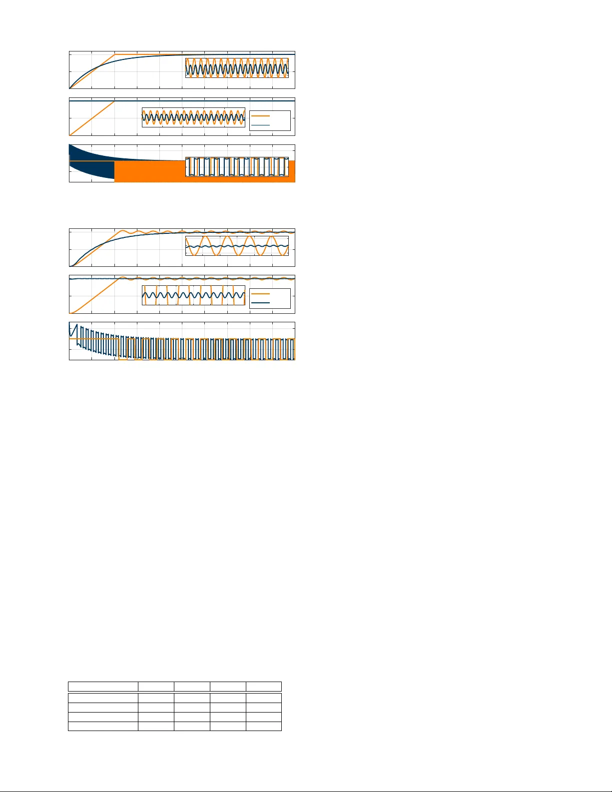
Chattering Reduction f or a Second-Order Actuator via Dynamic Sliding Manif olds Patricia N ¨ other , Lars W atermann and Johann Reger ⋆ Abstract — W e analyze actuator chattering in a scalar inte- grator system subject to second-order actuator dynamics with an unknown time constant and first-order sliding-mode control, using both a con ventional static sliding manifold and a dynamic sliding manifold. Using the harmonic balance method we proof that it is possible to adjust the parameters of the dynamic sliding manifold so as to reduce the amplitude of the chattering in comparison to the static manifold. The proof of concept is illustrated with an example. I . I N T RO D U C T I O N Sliding mode control (SMC) is a well-known approach for handling systems with bounded disturbances and un- certainties [1]. Ho wev er , a significant disadvantage is the occurrence of chattering, which is a high-frequency , periodic oscillation along the sliding manifold [2], [3]. Chattering is known to occur due to the discontinuity in the control signal. Common methods against this kind of chattering are the approximation of the discontinuity [4] and higher- order s liding modes by shifting the discontinuity into higher order deriv ativ es of the control [5]. Howe ver , in addition, chattering also occurs with continuous signals due to unmod- eled dynamics in the system [6], [7]. Especially , chattering is known to occur in first-order SMC with actuators of relativ e de gree two or higher [6]. T o suppress chattering caused by unmodeled dynamics, applying state observers [8] or filter characteristics [9] are discussed. In [10] chattering due to discontinuity is reduced by the approximation with a saturation function and the parameters of the control are tuned using the describing function method. Another approach for adjusting or improving the system behavior is using a dynamic sliding manifold (DSM) instead of a static sliding manifold (SSM). This method is adopted from frequency shaping sliding mode control [11]. F or example in [12], a DSM is applied to a boost and buck-boost con verter to stabilize the internal dynamics. Also in [13], the extra dynamics of the DSM are used as a compensator for the desired system behavior . In our previous study [14], we analyze stability with both globally bounded and unbounded perturbations using a DSM. The novel idea now is to use the DSM for reducing chattering compared to a SSM with similar performance properties, but without changing the switching law , i.e. without smoothening the sign-function, reducing the gain or increasing the order of the sliding mode. The analysis of the chattering is based on the so-called harmonic balance (HB) method or describing function (DF) All authors are with the Control Engineering Group, T echnische Univ er- sit ¨ at Ilmenau, P .O. Box 100565, D-98684, Ilmenau, Germany ⋆ Corresponding author: johann.reger@tu-ilmenau.de technique, rendering possible to calculate the amplitude and frequency of the fundamental oscillation [15]. The DF analysis in [16] shows that there is no chattering with a first- order stable lag in the unmodeled dynamics. The analysis is performed for ideal and real first-order SMC with a SSM. In this study , we give a proof of concept for applying a DSM to reduce chattering. W e show that, for a scalar integrator plant with second order actuator dynamics and unknown time constant, there is always a DSM that reduces the chattering amplitude. A simulation study underlines the result and demonstrates the effecti veness of the approach. The manuscript is structured as follows: In Section II we introduce the problem statement, and giv e the system class and the actuator structure. In Section III we analyze the chattering of the SSM and calculate its corresponding amplitude. The main results are presented in Section IV with the chattering analysis for the DSM and the proof of reducing the chattering amplitude for appropriate parameter selection in the DSM. These results are illustrated with a simulation example and various actuator values in Section V. Finally , we conclude with our results in Section VI. I I . P R O B L E M S TA T E M E N T Consider a scalar system ˙ x ( t ) = u ( t ) (1) with time t , state x ( t ) ∈ R , control input u ( t ) ∈ R and initial value x ( t 0 ) = x 0 at t 0 ≥ 0 . W e control this plant with a first-order SMC referring to the sliding manifold (SM) Ξ = { x ∈ R | σ ( x ( t )) = 0 } . The argument of the sliding varibale σ is omitted for the sake of readability . For the control design we choose the reaching law ˙ σ = − K sign ( σ ) (2) with control gain K > 0 to achieve finite-time conv ergence to the SM [1]. Additionally , assume a second order actuator  ˙ ξ 1 ( t ) ˙ ξ 2 ( t )  =  0 1 − 1 τ 2 − 2 τ   ξ 1 ( t ) ξ 2 ( t )  +  0 1 τ 2  u a ( t ) (3) with actuator state ξ ( t ) = ( ξ 1 ( t ) , ξ 2 ( t )) ⊤ ∈ R 2 , actuator input u a ( t ) ∈ R and initial value ξ ( t 0 ) = ξ 0 . The actuator output u ( t ) = ξ 1 ( t ) shall be the input to the plant (1). The actual control input is the input of the actuator . W e assume the structure (3) of the actuator to be kno wn, but the time constant τ unknown. Furthermore, we assume that the initial value of the actuator state is not known and that the actuator state is not measurable, hence not av ailable for control. The relativ e degree of the sliding variable σ with respect to the input u a is three. Thus, chattering is expected in the closed loop system [6]. The aim is to reduce the amplitude of the chattering by designing a ne w DSM with the same relativ e degree. All solutions of systems with discontinuities are understood in the sense of Filippov [17]. I I I . C H ATT E R I N G A N A L Y S I S F O R A S TA T I C S L I D I N G M A N I F O L D W e first shall design the control law for the ideal case without the actuator . A static sliding manifold (SSM) Ξ S = { x ∈ R | σ S ( x ( t )) = 0 } with σ S = x ( t ) (4) and the reaching law (2) yields the control law u ( t ) = − K sign( σ S ) (5) as input to the plant (1). W ith the actuator, the discontinuous control law (5) actually acts as the input u a to (3). T o analyze the chattering, we use the HB method [15]. W e follow the steps with unmodeled dynamics from [16]. T o this end, we extend the state of the plant (1) by the actuator states from (3) and insert control law (5). Replacing the nonlinearity sign( σ ) by an auxiliary input u HB we get the linear, partially closed loop system Σ S :                  ˙ x ˙ ξ 1 ˙ ξ 2   =   0 1 0 0 0 1 0 − 1 τ 2 − 2 τ     x ξ 1 ξ 2   +   0 0 − K τ 2   u HB σ S =  1 0 0    x ξ 1 ξ 2   (6) as depicted in Fig. 1. Note that, in this case, the partially closed loop is similar to the open loop (except for the factor − K ) because the equi v alent control vanishes for the integrator (1). The corresponding transfer function from auxiliary input u HB to output σ S is giv en by G S ( s ) = − K s ( s 2 τ 2 + 2 sτ + 1) . (7) Hence, applying the discontinuous input sign ( σ ) to the partially closed loop (6) leads to periodic oscillations in the system. Their fundamental oscillation is σ 1 ( t ) = ˆ σ sin ( ω p t ) . (8) with the amplitude ˆ σ > 0 and frequency ω p [15]. Assume that there is no phase shift in the oscillation of the sliding variable and that − σ = ˆ σ sin ( ω p t ) . (9) is valid [1]. T o determine the frequenc y ω p and the amplitude ˆ σ of the fundamental oscillation we intersect the negati ve in verse of the DF [1] of the nonlinearity sign( σ ) , that is N ( ˆ σ ) = 4 π ˆ σ (10) 1 u ( t ) σ ( t ) − 1 Σ ⋆ u HB ( t ) σ ( t ) − Fig. 1: Block diagram of the sign-function and the partially closed loop Σ ⋆ with ⋆ ∈ { S , D } . with (7) such that − 1 N ( ˆ σ ) = G S (i ω p ) . (11) First, we set the imaginary part of (7) to zero Im { G S (i ω p , S ) } = − K  ω 2 p , S τ 2 − 1  ω p , S  4 ω 2 p , S τ 2 +  ω 2 p , S τ 2 − 1  2  ≡ 0 (12) and receiv e the frequency ω p , S = 1 τ . (13) Inserting the frequency (13) into the real part of the transfer function (7), that is Re { G S (i ω ) } = 2 K τ 4 ω 2 τ 2 + ( ω 2 τ 2 − 1) 2 , (14) yields Re { G S (i ω p , S ) } = K τ 2 . (15) Then calculating the intersection of the HB (11) with (15) and the DF (10) leads to ˆ σ S = 2 K τ π (16) as chattering amplitude of the sliding variable. I V . D Y NA M I C S L I D I N G M A N I F O L D W e may adhere to the same procedure for analyzing the chattering calculation as before in Section III. Let the DSM Ξ D = { x ∈ R , z ∈ R | σ D ( x ( t ) , z ( t )) = 0 } be gi ven by ˙ z ( t ) = f z ( t ) + g x ( t ) (17a) σ D = hz ( t ) + lx ( t ) (17b) from [11] with design parameters f , g , h, l ∈ R . W e assume l  = 0 so as to keep the relativ e degree one from x to σ as in Section III. W ith the reaching law (2) we obtain the control law u ( t ) = − l − 1 ( K sign( σ D ) + hf z ( t ) + hg x ( t )) . (18) A. Stability Constraints The DSM (17) itself must be asymptotically stable, so we need f < 0 . Since the plant (1) does not contain perturbations, (18) with K > 0 guarantees the existence of the sliding mode [1], [11]. In sliding phase 0 ≡ σ , the reduced system with x ( t ) = − l − 1 hz ( t ) reads ˙ z ( t ) = ( f − g l − 1 h ) z ( t ) (19) and should be asymptotically stable without the influence of the actuator , hence f − g l − 1 h < 0 (20) is required for the design of the DSM. B. Chattering Analysis For the analysis with the DSM we calculate the partially closed loop equiv alent to Section III. Therefore, we extend the state x of (1) by the additional state z of the sliding manifold (17) and the actuator state ξ from (3). Inserting the control law (18) and again replacing sign( σ ) by the auxiliary input u HB we arriv e at the linear , partially closed loop Σ D :                                              ˙ z ˙ x ˙ ξ 1 ˙ ξ 2     =     f g 0 0 0 0 1 0 0 0 0 1 − hf lτ 2 − hg lτ 2 − 1 τ 2 − 2 τ         z x ξ 1 ξ 2     +     0 0 0 − K lτ 2     u HB σ D =  h l 0 0      z x ξ 1 ξ 2     . (21) Then the transfer function from input u HB to output σ D is G D ,σ ( s ) = − K ( g h − f l + ls ) s ( l τ 2 s 3 + a 2 s 2 + a 1 s + g h − f l ) (22) with parameters a 2 = (2 l τ − f l τ 2 ) , a 1 = l − 2 f lτ . The parameters f , g , h, l hav e to be selected such that l τ 2 s 3 + a 2 s 2 τ + a 1 s + g h − f l is a Hurwitz polynomial. This is especially fulfilled if f < 0 , sign( h ) = − sign( l ) and (20) holds. Theorem 1. F or system (1) subject to actuator dynamics (3) with τ unknown, a dynamic sliding manifold (17) can be chosen such that the chattering amplitude of the sliding variable σ is smaller than for the static sliding manifold (4) . Pr oof. W e choose scaled variables ˜ s := sτ , ˜ f := f τ and ˜ g := g τ according to [17]. The scaling of the parameter does not influence the stability constraints ˜ f − ˜ g l − 1 h =  f − g hl − 1  τ < 0 ⇔ f − g l − 1 h < 0 . (23) Additionally , we set h = − 1 and l = 1 . W ith the substitu- tions, the transfer function (22) simplifies to G D ,σ ( ˜ s ) = − K τ  ˜ f + ˜ g − ˜ s  ˜ s  − ˜ s 3 + ( ˜ f − 2) ˜ s 2 + (2 ˜ f − 1) ˜ s + ˜ f + ˜ g  . (24) Then we analyze the limit ˜ g → − ˜ f . Condition | ˜ g | < | ˜ f | must hold to satisfy the stability constraint (20). In the limit, the transfer function (24) is lim ˜ g →− ˜ f G D ,σ ( ˜ s ) = − K τ ˜ s  + ˜ s 2 + (2 − ˜ f ) ˜ s − 2 ˜ f + 1  . (25) Note that this limit cannot be reached. Y et, ˜ g can be chosen arbitrarily close to − ˜ f , hence, it is possible to get arbitrarily close to the limit. Calculating the intersection of the imaginary part of (25) with the real axis yields 0 = lim ˜ g →− ˜ f Im { G D ,σ (i ˜ ω p ) } = − K τ  ˜ ω 2 p + 2 ˜ f − 1  ˜ ω p   ˜ ω 2 p + 2 ˜ f − 1  2 +  2 ˜ ω p − ˜ f ˜ ω p  2  (26) ⇒ lim ˜ g →− ˜ f ˜ ω p , D = q 1 − 2 ˜ f . (27) Inserting (27) into the real part of the limit (25) gives lim ˜ g →− ˜ f Re { G D ,σ (i ˜ ω p , D ) } = K τ  2 − ˜ f   ˜ ω 2 p , D + 2 ˜ f − 1  2 +  2 ˜ ω p , D − ˜ f ˜ ω p , D  2 (28) = K τ 2 ˜ f 2 − 5 ˜ f + 2 (29) and equating with the negati ve in verse of the DF (10) yields the chattering amplitude lim ˜ g →− ˜ f ˆ σ D = 4 K τ π  2 ˜ f 2 − 5 ˜ f + 2  (30) of the sliding variable. Eventually , observe that lim ˜ g →− ˜ f ˆ σ D < ˆ σ S (31) ⇔ 4 K τ π  2 ˜ f 2 − 5 ˜ f + 2  < 2 K τ π (32) ⇔ 2 ˜ f 2 − 5 ˜ f > 0 , (33) which is fulfilled for all ˜ f < 0 , mimicking also one of the stability constraints. Remark 1. Note that ˜ f and ˜ g are unknown in general, but ar e scaled in the same way . So, the limit ˜ g → − ˜ f is equivalent to g → − f with f < 0 . W ith the selection l = 1 and h = − 1 all parameters can be chosen dir ectly . Note that − f should be selected sufficiently lar ge to over come the inaccuracies of the HB method. Remark 2. The selection of the parameters in the proof of Theor em 1 is only one possibility . T o avoid the limit, it is also feasible to set g = − α ˜ f , 0 < α < 1 and choose ˜ f . This appr oach leads to a mor e sophisticated analysis including a graphical comparison of the amplitudes. Sicne the sliding variables σ S and σ D correspond to distinct manifolds, the reduction of the chattering amplitude of the sliding variable does not guarantee the reduction of the chattering amplitude of the state in general, i.e., ˆ σ D < ˆ σ S does not ensure ˆ x D < ˆ x S . It is therefore essential to take the chattering of the state into account. Theorem 2. F or system (1) subject to actuator dynamics (3) with τ unknown, a dynamic sliding manifold (17) can be chosen such that the amplitude of the chattering of the state x ( t ) is smaller than for the static sliding manifold (4) . Pr oof. The amplitude of x with the SSM ˆ x S = ˆ σ S = 2 K τ π (34) is the same as (16). Due to the extended dynamics of (17b), the amplitude of x is different from that of σ d in the case with a DSM. Since the partially closed loop (21) is linear, the fundamental oscillation appears in all signals with the same frequency ω p . The amplitude and phase of the oscillation can be calculated by means of frequency domain analysis. T o calculate the amplitude of u HB we consider ˆ u HB = ˆ σ D | G D ,σ (i ω p ) | = ˆ σ D | Re { G D ,σ (i ω p ) }| = 4 π . (35) W e only need the absolute value of the real part because the imaginary part here is zero at ω p . Then we calculate the transfer function for system (21), but with ne w output y ( t ) = x ( t ) . (36) The transfer function from auxiliary input u HB ( t ) to x ( t ) is G D ,x ( s ) = K ( f − s ) s ( l τ 2 s 3 + a 2 s 2 + a 1 s + g h − f l ) (37) with a 2 = (2 lτ − f l τ 2 ) and a 1 = ( l − 2 f lτ ) . W e choose the same scaling of ˜ s , ˜ f and ˜ g , as well as the same selection h = − l = − 1 as in the proof of Theorem 1. Considering the limit for ˜ g → − ˜ f again yields lim ˜ g →− ˜ f G D , x ( ˜ s ) = K τ  ˜ f − ˜ s  ˜ s 2  ˜ s 2 + (2 − ˜ f ) ˜ s − 2 ˜ f + 1  (38) as limit of the new transfer function. Then, with the amplifi- cation of the transfer function (38) we calculate the amplitude lim ˜ g →− ˜ f ˆ x D = | G D ,x (i ω p , D ) | ˆ u HB (39) =        4 K τ  ˜ f − 1  π  1 − 2 ˜ f  1 / 2  2 ˜ f 2 − 5 ˜ f + 2         . (40) Re f G (j ! ) g -0 . 1 4 -0 . 1 2 -0.1 -0 . 0 8 -0 . 0 6 -0 . 0 4 -0 . 0 2 0 Im f G (j ! ) g -0 . 1 4 -0 . 1 2 -0 . 1 -0 . 0 8 -0 . 0 6 -0 . 0 4 -0 . 0 2 0 0.02 SSM = = 0 : 01 s SSM = = 0 : 1 s DSM = = 0 : 01 s DSM = = 0 : 1 s ! 1 N ! ^ < " -6 -4 -2 0 # 1 0 -3 -5 0 5 10 # 1 0 -4 Fig. 2: Harmonic Balance analysis for SMC and DSM each with τ = 0 . 01 s and τ = 0 . 1 s Eventually , we hav e to show that lim ˜ g →− ˜ f ˆ x D < ˆ x S (41) ⇔        2  ˜ f − 1   1 − 2 ˜ f  1 / 2  2 ˜ f 2 − 5 ˜ f + 2         < 1 . (42) Since ˜ f < 0 ,  1 − 2 ˜ f  1 2 > 1 also  2 ˜ f 2 − 5 ˜ f + 2  > 2(1 − ˜ f ) (43) holds. Hence, ˆ x D < ˆ x S holds for f < 0 with h = − 1 , l = 1 and g → − f . Since the selection of the parameters in Theorem 1 and Theorem 2 is the same, we have shown that it is possible to select f , g , h and l such that the amplitude of the chattering of both ˆ σ and ˆ x with the DSM is lower than for the SSM. V . E X A M P L E W e demonstrate the proposed method on two examples with τ ∈ { 0 . 01 , 0 . 1 } and K = 1 . As in the proof of Theorem 1 we choose h = − 1 and l = 1 . Since with limit g → − f the asymptotic stability of the reduced order dynamics is no longer valid in the sliding phase we set f = − 40 and g = 0 . 98 f = 39 . 6 . Like in integral SMC [18] we initialize the state z on the sliding manifold σ D ( t 0 ) = 0 , i.e. z 0 = x 0 . Hence, the reaching phase is eliminated. The HB analysis, Fig. 2, sho ws that the e xpected chattering amplitude of σ is significantly lo wer with the DSM than for the SSM. The amplitude increases with τ for the SSM. For ideal switching, i.e. with the sign -function, the amplitude of the DSM is lower for larger values of τ . Further, there is a margin between the real axis and the intersection between the local curves of the SSM and DSM. Hence, the approach may also be useful for chattering reduction in systems with nonideal switching, e.g. with a relay-function, whose negati ve inv erse of the describing function has a negati ve imaginary part. 0 1 2 3 4 5 6 7 8 9 10 x ( t ) -2 -1 0 0 1 2 3 4 5 6 7 8 9 10 < ( t ) -2 -1 0 SSM DSM t [s] 0 1 2 3 4 5 6 7 8 9 10 u ( t ) -1 0 1 2 9. 2 9. 4 9. 6 9. 8 -5 0 5 # 1 0 -3 9. 2 9. 4 9. 6 9. 8 -0.0 1 0 0. 01 9. 6 9. 7 9. 8 9. 9 -1 0 1 Fig. 3: Simulation with τ = 0 . 01 s 0 1 2 3 4 5 6 7 8 9 10 x ( t ) -2 -1 0 0 1 2 3 4 5 6 7 8 9 10 < ( t ) -2 -1 0 SSM DSM t [s] 0 1 2 3 4 5 6 7 8 9 10 u ( t ) -1 0 1 2 7. 5 8 8 .5 9 9. 5 -0.0 5 0 0. 05 7. 5 8 8 .5 9 9. 5 -0.0 1 0 0. 01 Fig. 4: Simulation with τ = 0 . 1 s In Fig. 3 and Fig. 4 the simulation with different τ is shown. The amplitude and frequency of the chattering depend on the actuator . With the selected parameters of the DSM, chattering both with respect to σ and x is significantly lower with the DSM than for the SSM. Ho wev er , the frequency in each scenario is higher with the DSM, which may cause problems in mechanical or electrical systems. If a possible interval for τ is known, f can be chosen considering the maximal acceptable frequency (27) of the interv al for τ . T able I compares the amplitudes of the simulation and cal- culation with ˆ σ from (16) and (30) and ˆ x from (34) and (40), respectiv ely . In this example, the calculated values for the SSM are slightly lower than those from the simulation. In this particular instance, the precision of the calculation with the HB is sufficiently high to obtain nearly identical results when comparing the scenario with the SSM and the DSM, both with the HB and the simulation. The magnitude of the HB analysis is consistent with that of the simulation. T ABLE I: Comparison of the chattering amplitudes in the analysis with HB and the simulation Scenario ˆ σ HB ˆ σ Sim. ˆ x HB ˆ x Sim. SSM, τ = 0 . 01 s 0 . 0064 0 . 0068 0 . 0064 0 . 0068 SSM, τ = 0 . 1 s 0 . 0637 0 . 0660 0 . 0637 0 . 0660 DSM, τ = 0 . 01 s 0 . 0029 0 . 0029 0 . 0031 0 . 0032 DSM, τ = 0 . 1 s 0 . 0024 0 . 0025 0 . 0039 0 . 0035 V I . C O N C L U S I O N W e analytically prov ed that it is always possible, for the given plant, to select DSM parameters such that the chattering amplitude of both the sliding variable and the state is reduced compared to the SSM. The e xample also illustrates that the reduction of chattering is indeed significant. The presented results represent a proof of concept and show that the proposed method is a promising novel technique for chattering reduction. In order to prepare the approach for practical applications, future research will address higher- dimensional systems and also take the control effort into account. R E F E R E N C E S [1] Y . Shtessel, C. Edwards, L. Fridman, and A. Lev ant, Sliding Mode Contr ol and Observation . Control Engineering, New Y ork, USA: Springer , 2014. [2] V . Utkin and Lee, Hoon, “Chattering Problem in Sliding Mode Control Systems, ” in International W orkshop on V ariable Structure Systems , (Alghero, Italy), pp. 346–350, IEEE, 2006. [3] A. Levant, “Chattering Analysis, ” IEEE T rans. Automat. Contr . , vol. 55, no. 6, pp. 1380–1389, 2010. [4] J. A. Burton and A. S. I. Zinober, “Continuous approximation of variable structure control, ” International Journal of Systems Science , vol. 17, pp. 875–885, June 1986. [5] G. Bartolini, A. Ferrara, and E. Usai, “Chattering avoidance by second- order sliding mode control, ” IEEE T rans. Automat. Contr . , vol. 43, no. 2, pp. 241–246, 1998. [6] I. Boiko and L. Fridman, “ Analysis of chattering in continuous sliding- mode controllers, ” IEEE T rans. Automat. Contr . , vol. 50, no. 9, pp. 1442–1446, 2005. [7] I. Boiko, L. Fridman, A. Pisano, and E. Usai, “ Analysis of Chattering in Systems With Second-Order Sliding Modes, ” IEEE T rans. Automat. Contr . , vol. 52, no. 11, pp. 2085–2102, 2007. [8] H. Lee and V . I. Utkin, “Chattering suppression methods in sliding mode control systems, ” Annual Reviews in Contr ol , vol. 31, no. 2, pp. 179–188, 2007. [9] D. Krupp and Y . B. Shtessel, “Chattering-free sliding mode control with unmodeled dynamics, ” in American Contr ol Conference , (San Diego, CA, USA), pp. 530–534 vol.1, IEEE, 1999. [10] I. Castillo and L. B. Freidovich, “Describing-function-based analysis to tune parameters of chattering reducing approximations of Sliding Mode controllers, ” Contr ol Engineering Practice , vol. 95, p. 104230, 2020. [11] K. D. Y oung and ¨ U. ¨ Ozg ¨ uner , “Frequency shaping compensator design for sliding mode, ” International Journal of Control , vol. 57, no. 5, pp. 1005–1019, 1993. [12] Y . B. Shtessel, A. S. I. Zinober, and I. A. Shkolnikov , “Sliding mode control of boost and buck-boost power conv erters using the dynamic sliding manifold, ” International Journal of Robust and Nonlinear Contr ol , vol. 13, no. 14, pp. 1285–1298, 2003. [13] A. Koshk ouei, K. Burnham, and A. Zinober , “Dynamic sliding mode control design, ” IEE Proc., Contr ol Theory Appl. , vol. 152, no. 4, pp. 392–396, 2005. [14] N. Tietze, K. W ulff, and J. Reger , “Local stability analysis for sliding mode control with unbounded perturbations – Dynamic sliding mode design revisited, ” in 64th Conference on Decision and Control , (Rio de Janeiro, Brazil), pp. 6975–6982, IEEE, 2025. [15] J.-J. E. Slotine and W . Li, Applied Nonlinear Control . Prentice Hall, 1991. [16] Y . B. Shtessel and Y .-J. Lee, “New Approach to Chattering Analysis in Systems with Sliding Modes, ” in 35th IEEE Conference on Decision and Control , vol. 4, pp. 4014–4019, 1996. [17] A. F . Filippov , Differ ential Equations with Discontinuous Righthand Sides: Control Systems . No. v .18 in Mathematics and Its Applications Ser, Dordrecht, Netherlands: Springer, 1988. [18] V . Utkin and J. Shi, “Integral Sliding Mode in Systems Operating un- der Uncertainty Conditions, ” in Confer ence on Decision and Contr ol , (K obe, Japan), 1996.