Room Impulse Response Completion Using Signal-Prediction Diffusion Models Conditioned on Simulated Early Reflections

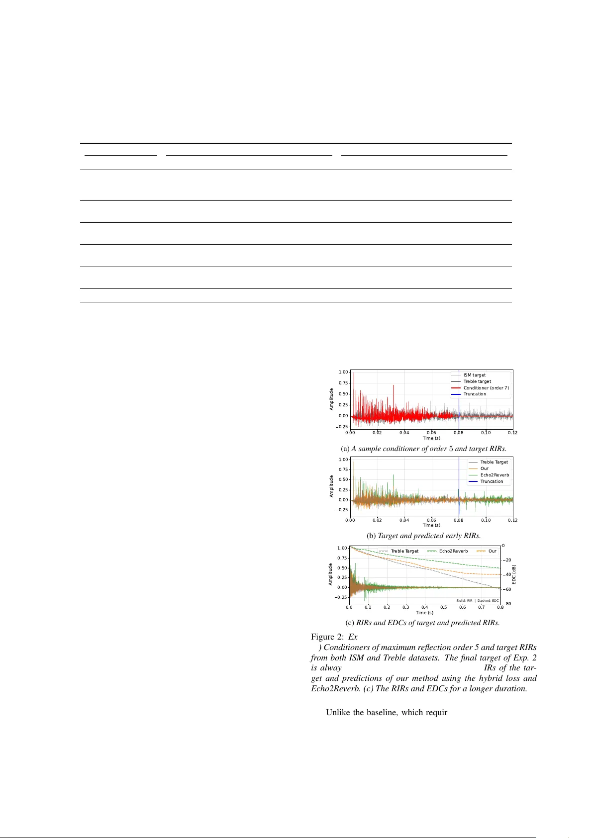
Room Impulse Response Completion Using Signal-Pr ediction Diffusion Models Conditioned on Simulated Early Reflections Ze yu Xu ID 1 , ∗∗ , Andr eas Br endel ID 2 , Albert G. Prinn ID 1 , Emanu ¨ el A. P . Habets ID 1 1 International Audio Laboratories Erlangen † , Germany 2 Fraunhofer Institute for Integrated Circuits (IIS), Erlangen, German y † A joint institution of the Friedrich-Alexander -Univ ersit ¨ at Erlangen-N ¨ urnberg (F A U) and Fraunhofer Institute for Integrated Circuits (IIS) zeyu.xu@audiolabs-erlangen.de Abstract Room impulse responses (RIRs) are fundamental to audio data augmentation, acoustic signal processing, and immersiv e audio rendering. While geometric simulators such as the image source method (ISM) can efficiently generate early reflections, they lack the realism of measured RIRs due to missing acoustic wa ve effects. W e propose a dif fusion-based RIR completion method using signal-prediction conditioned on ISM-simulated direct- path and early reflections. Unlike state-of-the-art methods, our approach imposes no fixed duration constraint on the input early reflections. W e further incorporate classifier-free guidance to steer generation toward a tar get distribution learned from phys- ically realistic RIRs simulated with the T reble SDK. Objectiv e ev aluation demonstrates that the proposed method outperforms a state-of-the-art baseline in early RIR completion and ener gy decay curve reconstruction. Index T erms : diffusion models, room impulse response com- pletion, image source method, classifier-free guidance 1. Introduction The generation of room impulse responses, RIRs, is central to immersiv e spatial audio rendering, acoustic array signal pro- cessing, and the construction of large scale machine learning datasets. T raditional physics based methods are broadly clas- sified into geometrical and numerical wa ve methods. Geomet- rical methods, including the image source method, ISM [1–3], ray tracing [4], beam tracing [5], and delay networks [6], model individual reflection paths. Numerical wav e methods instead solve the discretized wave equation using finite dif ference time domain [7], finite element [8], boundary element [9], or finite volume techniques [10]. Recently , deep learning approaches such as neural acoustic field models [11], Fast RIR [12], and physics informed neural network RIR [13] ha ve been proposed in the literature. More recently , RIR completion has emerged as a new task in RIR generation, aiming to complete the full RIR after a 50 ms [14] or 80 ms [15] windo w (RIR head), comprising the direct path and early reflections, with the direct-path delay re- mov ed. This new task assumes that the direct path and early reflections contain sufficient information about the room, i.e., its geometry and wall materials, to predict the late part of the RIR. Howe ver , existing state-of-the-art methods for RIR com- pletion [14, 15] typically require an RIR-head input truncated from a fully simulated or measured RIR, whereas many geomet- ric RIR simulation implementations, e.g., the ISM [16, 17], ac- ** indicates the corresponding author . cept the maximum reflection order as an input parameter . This is a limitation of existing methods, as using an incomplete RIR head from a low-order ISM simulation would lead to disconti- nuities in the completed RIR. W ithin generativ e modeling, diffusion models [18] offer a powerful frame work for learning comple x data distributions and hav e recently been applied to RIR tasks. Examples include DiffusionRIR [19], which interpolates RIRs at unseen posi- tions, and Gencho [20], which estimates RIRs from rev erberant speech. A central design choice in dif fusion models is the tar- get predicted at each dif fusion step. The original DDPM formu- lation [18] introduced noise prediction, which remains popular due to its stable training dynamics. Ho wev er , equi v alent param- eterizations exist, including velocity prediction ( v -prediction), as adopted in Gencho [20]. Despite these advances, current diffusion-based RIR approaches focus on interpolation or full RIR estimation, and RIR completion methods typically rely on complete early-reflection information. T o date, there is no dif- fusion frame work tailored to RIR completion from incomplete early responses, nor a systematic in vestig ation of applying sig- nal prediction ( x -prediction) as the target in diffusion models for generating physically coherent RIRs without discontinuities under partial conditioning. This paper proposes an RIR completion method based on an x -prediction diffusion model conditioned solely on simulated direct-path and early reflections obtained from the ISM. The proposed approach generates a complete full-band RIR even when the RIR head is incomplete, whereas existing methods may introduce temporal discontinuities. In particular , it does not require access to the truncated early reflections of a fully simulated or measured RIR. T o more accurately assess the per- formance of the proposed method under realistic conditions, two paired datasets with identical room configurations are con- structed for classifier-free guidance (CFG) training: one con- sisting solely of ISM simulations and the other comprising RIRs simulated using a numerical wav e method. When trained with CFG, the model produces more realistic RIRs than a baseline diffusion model, e ven when the training data are dominated by ISM-simulated RIRs that lack wav e interference effects and in- clude only a small proportion of realistic examples. Further- more, incorporating an energy decay curv e (EDC) loss [21] im- prov es the preservation of physically consistent energy decay characteristics. 2. Proposed Method 2.1. Conditioned Diffusion Models with x -Prediction W e define the noise-free target RIR of length K as x 0 ∈ R K , and noisy RIR at time step t in the forward and backward diffusion as x t ∈ R K . The forward diffusion process for t = 1 , . . . , T can be written as x t = √ ¯ α t x 0 + √ 1 − ¯ α t ϵ t , (1) where ϵ t ∼ N ( 0 , I ) is the added standard Gaussian noise in R K , and ¯ α t = Q t t ′ =1 α t ′ is the accumulated signal retention after t time steps and α t ′ is the signal retention at time step t ′ . They are obtained using the cosine schedule [22]. W e aim to reconstruct the target RIR x 0 using a result of a low-order ISM simulation c ∈ R K as the conditioner of the diffusion model. For x -prediction, the neural network X θ ( · ) parameterized by θ is trained to directly predict the tar get RIR x 0 in (1), i.e., ˆ x 0 = X θ ( x t , c , t ) ≈ x 0 . During inference, the same noise schedule as in training is employed, and the update x t − 1 = µ θ ( x t , t ) + σ t ϵ t is applied recursi vely . The rev erse mean µ θ ( x t , t ) is calculated using µ θ ( x t , t ) = √ ¯ α t − 1 (1 − α t ) 1 − ¯ α t ˆ x 0 + √ α t  1 − ¯ α t − 1  1 − ¯ α t x t , (2) where the standard de viation is σ t = q (1 − ¯ α t − 1 )(1 − α t ) 1 − ¯ α t , and the noise ϵ t is not added in the last step. 2.2. Network Structure W e use the 1D U-Net architecture [18] to predict the tar get RIR x 0 from the noisy sample x t within the diffusion process. The ISM-based conditioning signal c is concatenated with x t along the channel dimension, yielding the input [ c , x t ] ∈ R K × 2 . T wo major modifications are made to the 1D U-Net proposed in [18]: i) The required do wnsampling factor of the U-Net encoder de- pends on the maximum RIR length and the target bottleneck length. In our model, 7 stride-2 downsamples are applied, sup- porting up to 32 768 RIR samples and a bottleneck length of 256 . ii) In the bottleneck, a 6-layer residual dilated Conv1D stack with dilations 1 , 2 , 4 , 8 , 16 , 32 is applied to capture long- range temporal structure, such as late rev erberation. 2.3. Loss Functions For the model output ˆ x 0 = [ ˆ x 0 [0] , ˆ x 0 [1] , . . . , ˆ x 0 [ K − 1]] T and the target x 0 = [ x 0 [0] , x 0 [1] , . . . , x 0 [ K − 1]] T , the MSE loss is giv en by L MSE = 1 K K − 1 X n =0 ( x 0 [ n ] − ˆ x 0 [ n ]) 2 . (3) The EDC of an RIR x 0 can be calculated using a discrete version of Schroeder’ s backward integration [23]: E [ n ] = P K − 1 k = n x 2 0 [ k ] for n = 0 , 1 , . . . , K − 1 . The normal- ized EDC in logarithmic scale is gi ven by E dB [ n ] = 10 log 10 ( E [ n ] /E [0]) . The EDC is further clamped by setting E dB [ n ] = max( E dB [ n ] , E min ) with E min = − 60 dB. W ith the EDCs of the predicted and target RIRs, gi ven by b E dB and E dB , respectiv ely , we calculate the EDC loss as L EDC = K − 1 X n =0 w [ n ]    b E dB [ n ] − E dB [ n ]    , (4) where w [ n ] forms a normalized uniform weighting ov er time samples for which E dB [ n ] ≥ − 60 . The total loss is a weighted combination of the MSE and EDC loss L total = L MSE + λ L EDC , (5) where λ ≥ 0 is a scaling factor . 2.4. Classifier-Fr ee Guidance For CFG [24], we train a single denoising netw ork to operate in both conditional and unconditional mode by randomly replac- ing the conditioner with an all-zero vector c = 0 ∈ R K with probability p CFG . This conditioning dropout forces the model to jointly learn the conditional and unconditional RIR distribution guided by the early reflections. At inference, we apply CFG by ev aluating the denoiser twice per reverse step, once with the conditioning signal and once with the null condition. W ith the two predictions in each reverse diffusion step, ˆ x c 0 = X θ ( x t , c , t ) and ˆ x uc 0 = X θ ( x t , 0 , t ) , the combined prediction is ˆ x CFG 0 = ˆ x uc 0 + s ( ˆ x c 0 − ˆ x uc 0 ) , (6) where s ≥ 1 is the guidance scale that controls the tradeoff between condition adherence and sample div ersity . 3. Experimental Setup 3.1. Datasets T wo paired RIR datasets were generated for 25 shoebox rooms with randomly sampled dimensions under consistent simula- tion conditions using pyroomacoustics [17] and the T reble SDK [25]. Floor materials were randomly selected from car- pet types, while the ceiling and four walls were randomly as- signed gypsum-based materials. For the Treble SDK dataset only , one upholstered sof a, two wooden chairs, and one w ooden table were randomly placed on the floor , with identical furniture materials across rooms. Each room contained 10 point sources and 40 omnidirectional receiv ers, all positioned randomly , sub- ject to a minimum distance from the walls and furniture. The dataset generated using only the ISM in pyroomacous- tics is referred to as the ISM dataset , whereas the dataset gener - ated using both geometric and numerical w av e simulation in the T reble SDK is referred to as the T r eble dataset . It has recently been shown that RIRs produced with the numerical wav e sim- ulator in the T reble SDK enable learning-based acoustic signal processing methods to achie ve performance comparable to that obtained with measured RIRs [26]. Importantly , room geome- try , wall absorption coefficients, and source and recei ver posi- tions are identical across the two datasets. The T reble dataset additionally captures wav e interference due to furniture as well as diffraction at edges and corners. Each dataset comprised 10 000 RIRs and was randomly split in an 8 : 1 : 1 ratio into training, v alidation, and test sets. All RIRs were normalized to unit peak amplitude. Direct-path delays were removed from both RIRs and conditioning signals, except for a 2 . 5 ms segment retained to preserv e the first arriv al. RIRs were truncated or zero-padded to K = 24 576 samples, corresponding to 1 . 536 s at a sampling rate of 16 kHz. Since the original Echo2Rev erb implementation performs RIR completion up to 2 . 5 s at 48 kHz, all signals were first upsampled from 16 kHz to 48 kHz and zero-padded to match the required length. After inference, the generated outputs were low-pass filtered, downsampled, and truncated to K = 24 576 samples for ev aluation. 0.00 0.02 0.04 0.06 0.08 0.10 0.12 T ime (s) 0.25 0.00 0.25 0.50 0.75 1.00 Amplitude RIR (total) Or der 7 Or der 5 Or der 3 Or der 1 T runcation Figure 1: Examples of ISM conditioners with dif fer ent maximum r eflection order s 1 , 3 , 5 , 7 and the full RIR. The conditioners ar e truncated to 80 ms such that they can be used as inputs to both the pr oposed model and Echo2Reverb . 3.2. Conditioner Configurations The baseline model Echo2Re verb [15] used the first 80 ms of a full RIR as conditioning input to generate late re verberation. In practice, howev er , early reflections simulated with the ISM can be obtained more ef ficiently by specifying a maximum re- flection order rather than a fixed time window . Accordingly , ISM-based conditioners c of length 80 ms were generated with maximum reflection orders of 1 , 3 , 5 , and 7 . T o remain consis- tent with the original baseline configuration, Echo2Reverb was conditioned on early reflections obtained by truncating the full RIR to 80 ms. In addition, to ev aluate its behavior under order - limited conditions, ISM conditioners with reflection orders 5 and 7 were also provided as inputs. The ISM conditioners were generated using the same room parameters as those employed for full RIR simulation in the ISM dataset. Examples of trun- cated ISM conditioners are shown in Fig. 1. Notably , e ven a reflection order of 7 does not fully populate the 80 ms windo w . The proposed model does not require truncation of the condi- tioning signal. 3.3. Experiments T wo experiments were conducted to evaluate the proposed method and Echo2Rev erb . In the first experiment, only the ISM dataset was used. In the second experiment, a combined dataset was constructed by randomly selecting from the ISM and Treble datasets with a ratio of 8 : 2 for training and v ali- dation. Only the Treble dataset was used for testing. The CFG probability p CFG was set to 0 . 2 during training and v alidation. Echo2Rev erb was trained and validated using the same dataset configuration; howe ver , in contrast to the CFG-based training pipeline of the proposed method, the conditioning signals were not dropped. For the proposed method, the guidance scale was set to 1 during inference, corresponding to fully conditioned sampling. Across both experiments, the maximum reflection order of the ISM conditioner (described in Sec. 3.2) was varied. Furthermore, the proposed model was trained using either the MSE loss (3) or the total loss (5) with an empirically chosen scaling factor λ = 10 − 5 . 4. Evaluation 4.1. Metrics W e ev aluated reconstruction errors between the predicted RIR ˆ x 0 and the noise-free tar get RIR x 0 for dif ferent sections of the RIRs. The first section covers the early 80 ms windo w , where the conditioner c may overlap with the full RIR, as shown in Fig. 1. The objecti ve is to quantify the mismatch between the predicted and target RIRs only in the residual components, i.e., between r = x − c and ˆ r = ˆ x − c . Since the ISM conditioner may span the 80 ms window differently as the maximum reflec- tion order changes, we calculated the follo wing residual ener gy ratio (RER) for the early 80 ms RIR ≤ 80 RER = P K 80 − 1 n =0 ˆ r [ n ] 2 P K 80 − 1 n =0 r [ n ] 2 , (7) where K 80 denotes the first time sample after the conditioner window . A value of around 1 of the RER indicates that the residual of the completed RIR and the conditioner contains a similar amount of energy as the residual of the target RIR in the 80 ms window . For the RIR completion error after 80 ms, the root mean square error (RMSE) RIR > 80 RMSE = v u u t 1 K − K 80 K − 1 X n = K 80 ( ˆ x [ n ] − x [ n ]) 2 (8) was calculated. T o measure the accuracy in terms of the EDC, the mean absolute error (MAE) w as calculated between the tar - get EDC E dB [ n ] and the predicted EDC b E dB [ n ] for the time samples where E dB [ n ] ≥ − 60 dB EDC MAE = K − 1 X n =0 w [ n ]    b E dB [ n ] − E dB [ n ]    , (9) where w [ n ] is the same as used in (4). Note that all three error metrics are reported in dB. 4.2. Experiment 1: ISM RIRs The objecti ve ev aluation over the ISM dataset is illustrated as Exp. 1 in T ab. 1, where the mean and standard deviation of the three metrics are giv en for the proposed and baseline models. For the proposed model, the three metrics do not v ary sig- nificantly as the maximum reflection order of the input ISM conditioner changes. Ho we ver , including the EDC loss (5) low- ers EDC MAE significantly relativ e to using only the MSE loss in training. When the ISM conditioner is of order 5, the best EDC errors in our model are slightly worse than those of the Echo2Rev erb model fed by the same ISM conditioner . When the ISM conditioner’ s order increases to 7 , the early RER er- ror RIR ≤ 80 RER is lower than for the Echo2Re verb with the same conditioner when the hybrid loss is used in our method. 4.3. Experiment 2: CFG training with combined dataset In the following, the ISM dataset is also compared with the Tre- ble dataset to demonstrate the intrinsic dataset mismatch be- tween the two datasets, which provides a cross-dataset discrep- ancy baseline. In this case, the ISM dataset and T reble dataset are used as the prediction and target, respectiv ely . The discrep- ancy baseline is illustrated as the last ro w in T ab. 1 for the in- put conditioner of maximum reflection order 7, which almost fills the early 80 ms window , leaving little room for early RIR completion. It is clear that both our method and Echo2Rev erb outperform the discrepancy baseline at most configurations for all three metrics, except that our method may have worse EDC error when the conditioner is of order 1. Now , the early RER RIR ≤ 80 RER changes substantially with the maximum reflection or - der for our method. When the orders are 1 , 3 , 5 , the early RERs of our method are all better than those in Echo2Reverb . Note that in Exp. 1, this performance advantage is not as obvi- ous since the conditioner and the target are both from the ISM dataset, sharing very close early reflection patterns, as also ob- served in Fig. 1. Howe ver , in Exp. 2, the Treble dataset is used T able 1: P erformance comparison between our pr oposed model and the baseline model Echo2Reverb for the two experiments. M denotes that only the MSE loss was used. M+E indicates that both the EDC and the MSE losses wer e used. The numbers 1 , 3 , 5 , 7 and Full denote the maximum r eflection order in the ISM conditioner , used as input to the trained model. F or each entry, mean (standar d deviation) values ar e shown. Arr ow ↓ indicates lower values ar e better , and 0 indicates that values closer to 0 are better . The best value in each column is highlighted for Ec ho2Reverb and our method. The RIRs of the ISM dataset ar e also compar ed against the metrics in Exp. 2 to demonstrate the intrinsic dataset mismatc h between the ISM and T reble datasets, despite equal r oom configurations. Source Exp. 1: ISM dataset Exp. 2: CFG training with the combined dataset Method Order RIR ≤ 80 RER ( dB , 0 ) RIR > 80 RMSE ( dB , ↓ ) EDC MAE ( dB , ↓ ) RIR ≤ 80 RER ( dB , 0 ) RIR > 80 RMSE ( dB , ↓ ) EDC MAE ( dB , ↓ ) Echo2Rev erb 5 -3.73 (6.11) -21.09 (6.11) -1.01 (3.36) -12.21 (1.96) -21.95 (5.35) 9.46 (3.75) Echo2Rev erb 7 2.57 (7.09) -21.14 (6.14) -0.35 (3.73) -12.18 (1.83) -22.06 (5.41) 9.62 (3.56) Echo2Rev erb Full – -21.18 (6.15) 0.73 (4.24) -12.06 (1.72) -22.07 (5.47) 9.62 (3.53) Proposed M 1 -1.54 (1.54) -21.63 (5.82) 9.54 (2.19) -1.94 (2.14) -23.92 (4.80) 10.23 (1.53) Proposed M+E 1 1.43 (2.36) -20.53 (5.58) 3.61 (3.23) -1.25 (1.86) -21.46 (3.77) 11.80 (2.68) Proposed M 3 -5.13 (1.98) -22.12 (5.77) 10.59 (1.43) -3.45 (5.78) -22.62 (5.48) 10.25 (1.90) Proposed M+E 3 2.21 (2.49) -20.38 (5.37) 2.75 (4.35) -1.29 (3.26) -21.90 (4.23) 9.37 (3.23) Proposed M 5 -3.85 (4.78) -21.50 (5.93) 9.09 (1.95) -9.24 (7.76) -23.47 (4.94) 9.66 (1.81) Proposed M+E 5 -2.72 (2.82) -21.32 (5.99) 0.81 (2.01) -6.64 (5.22) -22.38 (4.07) 9.30 (2.69) Proposed M 7 -3.12 (2.65) -21.74 (6.02) 8.49 (1.79) -13.02 (8.65) -22.74 (5.57) 9.00 (1.61) Proposed M+E 7 -0.05 (3.23) -20.90 (6.00) 1.35 (2.65) -13.00 (7.86) -22.95 (4.49) 8.66 (3.80) ISM Dataset 7 – – – -14.76 (5.92) -21.86 (5.36) 10.09 (3.30) as the target. An example comparison of the early RIRs be- tween the ISM and T reble datasets is in Fig. 2a, indicating that differences are already visible e ven in the 80 ms window due to the additional acoustic effects, e.g., reflections and diffractions caused by furniture. Since Echo2Rev erb does not improve the 80 ms window , the advantageous performance of our method is clearly showcased when the target RIR is from a different dataset to the conditioner . Howe ver , when the reflection order of the conditioner increases in our method, e.g., at order 7 , the RER v alues also get worse since there is little room to complete the 80 ms windo w . Our method and Echo2Rev erb are compet- itiv e regarding the RMSE errors RIR > 80 RMSE , which is similar to the observation in Exp. 1. But the EDC error EDC MAE of our methods for conditioner orders 5 and 7 is clearly lower than Echo2Rev erb in terms of mean value and standard deviation. An example of the predictions of our method and Echo2Re verb is shown in Fig. 2b and Fig. 2c. The predictions of Echo2Rev erb may contain a discontinuity if the 80 ms window is not filled with early reflections. Since it directly takes the conditioner from the ISM dataset as the early parts of the output, early completion errors are much more severe, which can be con- firmed by the RER RIR ≤ 80 RER in T ab. 1. T o maintain the o verall shape of the EDC curve, Echo2Rev erb produces spurious large- amplitude pulses after the 80 ms window , while our method can generate smooth RIR decay regardless of the conditioner’ s re- flection order and duration. Overall, the EDC of our method is closer to the target EDC compared to Echo2Rev erb, ev en though Echo2Reverb is very good at predicting the EDCs, as observed in Exp. 1. The observ ations in Exp. 2 highlight the ad- vantages of our method with the CFG training, that e ven when the input conditioner is dropped out at a ratio of 0 . 2 , our method achiev es better early completion of RIRs and EDC fitting than Echo2Rev erb, which is trained without conditioner dropout. 5. Conclusions W e proposed an x -prediction diffusion model conditioned on simulated early reflections for RIR completion. Evaluated on two datasets, i.e., an ISM dataset and a more realistic Treble dataset, our method matches the baseline when trained on ISM data alone. When trained with CFG on a hybrid dataset (80% ISM, 20% Treble) and tested on an unseen subset of the Treble dataset, it outperforms the baseline in early-reflection comple- tion and energy decay curve reconstruction, provided that con- sistent input conditioners are used. 0.00 0.02 0.04 0.06 0.08 0.10 0.12 T ime (s) 0.25 0.00 0.25 0.50 0.75 1.00 Amplitude ISM tar get T r eble tar get Conditioner (or der 7) T runcation (a) A sample conditioner of or der 5 and target RIRs. 0.00 0.02 0.04 0.06 0.08 0.10 0.12 T ime (s) 0.25 0.00 0.25 0.50 0.75 1.00 Amplitude T r eble T ar get Our Echo2R everb T runcation (b) T ar get and predicted early RIRs. 0.0 0.1 0.2 0.3 0.4 0.5 0.6 0.7 0.8 T ime (s) 0.25 0.00 0.25 0.50 0.75 1.00 Amplitude Solid: RIR | Dashed: EDC T r eble T ar get Echo2R everb Our 80 60 40 20 0 EDC (dB) (c) RIRs and EDCs of tar get and pr edicted RIRs. Figure 2: Example comparisons in the test dataset for Exp. 2. (a) Conditioner s of maximum reflection or der 5 and tar get RIRs fr om both ISM and T r eble datasets. The final target of Exp. 2 is always fr om the T reble dataset. (b) Early RIRs of the tar- get and predictions of our method using the hybrid loss and Echo2Re verb . (c) The RIRs and EDCs for a longer duration. Unlike the baseline, which requires complete early reflec- tions within an 80 ms window , our method accommodates lower -order ISM simulations down to first-order reflections. These results demonstrate the viability of generating realistic RIRs from only the direct path and low-order early reflections. Future work includes improving performance at very lo w re- flection orders and accelerating dif fusion model inference, both of which are critical for practical deployment. 6. References [1] J. B. Allen and D. A. Berkley , “Image method for efficiently sim- ulating small-room acoustics, ” J. Acoust. Soc. Am. , vol. 65, no. 4, pp. 943–950, 1979. [2] J. Borish, “Extension of the image model to arbitrary polyhedra, ” J. Acoust. Soc. Am. , v ol. 75, no. 6, pp. 1827–1836, Jun. 1984. [3] Z. Xu, A. Herzog, A. Lodermeyer , E. A. P . Habets, and A. G. Prinn, “Simulating room transfer functions between transduc- ers mounted on audio devices using a modified image source method, ” J. Acoust. Soc. Am. , v ol. 155, pp. 343–357, Jan. 2024. [4] A. Krokstad, S. Strom, and S. Sørsdal, “Calculating the acoustical room response by the use of a ray tracing technique, ” J. Sound V ib . , vol. 8, no. 1, pp. 118–125, 1968. [5] T . Funkhouser , N. Tsingos, I. Carlbom, G. Elko, M. Sondhi, J. E. W est, G. Pingali, P . Min, and A. Ngan, “ A beam tracing method for interactive architectural acoustics, ” J. Acoust. Soc. Am. , vol. 115, no. 2, pp. 739–756, 2004. [6] J.-M. Jot and A. Chaigne, “Digital delay networks for designing artificial re verberators, ” in A udio Engineering Society Convention . Audio Engineering Society , 1991. [7] D. Botteldooren, “Finite-difference time-domain simulation of low-frequenc y room acoustic problems, ” J. Acoust. Soc. Am. , vol. 98, no. 6, pp. 3302–3308, 1995. [8] T . Shuku and K. Ishihara, “The analysis of the acoustic field in irregularly shaped rooms by the finite element method, ” J. Sound V ib . , vol. 29, no. 1, pp. 67–76, 1973. [9] M. R. Bai, “ Application of bem (boundary element method)-based acoustic holography to radiation analysis of sound sources with arbitrarily shaped geometries, ” J . Acoust. Soc. Am. , v ol. 92, no. 1, pp. 533–549, 1992. [10] S. Bilbao, B. Hamilton, J. Botts, and L. Savioja, “Finite volume time domain room acoustics simulation under general impedance boundary conditions, ” IEEE/A CM T ransactions on Audio, Speech, and Language Pr ocessing , vol. 24, no. 1, pp. 161–173, 2015. [11] A. Luo, Y . Du, M. T arr, J. T enenbaum, A. T orralba, and C. Gan, “Learning neural acoustic fields, ” Advances in Neural Information Pr ocessing Systems , v ol. 35, pp. 3165–3177, 2022. [12] A. Ratnarajah, S.-X. Zhang, M. Y u, Z. T ang, D. Manocha, and D. Y u, “F ast-RIR: Fast neural diffuse room impulse response gen- erator , ” in IEEE International Conference on Acoustics, Speech and Signal Pr ocessing (ICASSP) , 2022, pp. 571–575. [13] X. Karakonstantis, D. Ca viedes-Nozal, A. Richard, and E. Fernandez-Grande, “Room impulse response reconstruction with physics-informed deep learning, ” J. Acoust. Soc. Am. , v ol. 155, no. 2, pp. 1048–1059, 2024. [14] J. Lin, G. G ¨ otz, and S. J. Schlecht, “Deep room impulse response completion, ” EURASIP Journal on Audio, Speech, and Music Pr ocessing , v ol. 2025, no. 1, p. 20, 2025. [15] S. Kim, J.-h. Y oo, and J.-W . Choi, “Echo-aware room impulse response generation, ” J. Acoust. Soc. Am. , vol. 156, no. 1, pp. 623–637, 2024. [16] E. A. P . Habets, “Room impulse response generator , ” T ec hnische Universiteit Eindhoven, T ech. Rep. , pp. 1–16, 2006. [17] R. Scheibler , E. Bezzam, and I. Dokmani ´ c, “Pyroomacoustics: A python package for audio room simulation and array process- ing algorithms, ” in IEEE International Confer ence on Acoustics, Speech and Signal Pr ocessing (ICASSP) , 2018, pp. 351–355. [18] J. Ho, A. Jain, and P . Abbeel, “Denoising diffusion probabilis- tic models, ” Advances in neural information pr ocessing systems , vol. 33, pp. 6840–6851, 2020. [19] S. Della T orre, M. Pezzoli, F . Antonacci, and S. Gannot, “Dif- fusionRIR: Room impulse response interpolation using dif fusion models, ” arXiv preprint , 2025. [20] J. Lin, J. Su, N. Anand, Z. Jin, M. Kim, and P . Smaragdis, “Gencho: Room impulse response generation from reverber - ant speech and text via diffusion transformers, ” arXiv preprint arXiv:2602.09233 , 2026. [21] A. I. Mezza, R. Giampiccolo, A. Bernardini et al. , “Dif ferentiable scattering delay networks for artificial reverberation, ” in Interna- tional Confer ence on Digital Audio Effects (DAFx25) , 2025, pp. 202–207. [22] A. Q. Nichol and P . Dhariwal, “Improved denoising diffusion probabilistic models, ” in International conference on machine learning . PMLR, 2021, pp. 8162–8171. [23] M. R. Schroeder , “New method of measuring rev erberation time, ” J. Acoust. Soc. Am. , v ol. 37, no. 3, pp. 409–412, 1965. [24] J. Ho and T . Salimans, “Classifier-free dif fusion guidance, ” arXiv pr eprint arXiv:2207.12598 , 2022. [25] Treble T echnologies, “Treble SDK documentation, ” https://docs. treble.tech/treble- sdk/, 2026, accessed: 2026-03-02. [26] G. G ¨ otz, D. G. Nielsen, S. Gudj ´ onsson, and F . Pind, “Room- acoustic simulations as an alternative to measurements for audio- algorithm evaluation, ” IEEE Access , vol. 13, pp. 214 000– 214 008, 2025.