Descent-Guided Policy Gradient for Scalable Cooperative Multi-Agent Learning

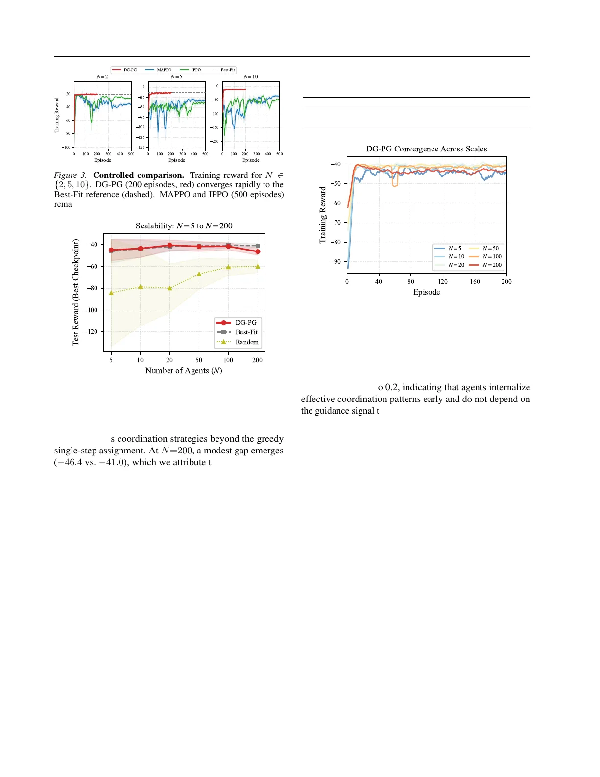
Descent-Guided P olicy Gradient f or Scalable Cooperativ e Multi-Agent Learning Shan Y ang 1 Y ang Liu 2 1 Abstract Scaling cooperativ e multi-agent reinforcement learning (MARL) is fundamentally limited by cross-agent noise. When agents share a common rew ard, the actions of all N agents jointly deter- mine each agent’ s learning signal, so cross-agent noise gro ws with N . In the polic y gradient set- ting, per-agent gradient estimate v ariance scales as Θ( N ) , yielding sample complexity O ( N/ϵ ) . W e observe that man y domains, including cloud computing, transportation, and po wer systems, hav e dif ferentiable analytical models that pre- scribe efﬁcient system states. In this work, we propose Descent-Guided Polic y Gradient (DG- PG), a framework that utilizes these analytical models to provide each agent with a noise-free gradient signal, decoupling each agent’ s gradient from the actions of all others. W e prove that DG- PG reduces gradient variance from Θ( N ) to O (1) , preserves the equilibria of the cooperati ve game, and achiev es agent-independent sample complex- ity O (1 /ϵ ) . On a heterogeneous cloud scheduling task with up to 200 agents, DG-PG con ver ges within 10 episodes at ev ery tested scale, from N =5 to N =200 , directly conﬁrming the pre- dicted scale-in variant complexity , while MAPPO and IPPO fail to conv erge under identical archi- tectures. 1. Introduction Multi-agent reinforcement learning (MARL) has demon- strated remarkable success across a wide range of domains, from game playing ( Y u et al. , 2022 ) to cloud resource scheduling ( Mao et al. , 2019 ) and transportation manage- ment ( El-T antawy et al. , 2013 ). In many of these applica- tions, agents share a common objecti ve and must coordinate 1 Department of Industrial Systems Engineering and Manage- ment, National Uni versity of Singapore, Singapore 2 Department of Civil and En vironmental Engineering, National Univ ersity of Singapore, Singapore. Correspondence to: Y ang Shan < yang shan@u.nus.edu > , Liu Y ang < ceelya@nus.edu.sg > . Pr eprint. Marc h 18, 2026. their beha vior , a setting known as cooperati ve MARL. How- ev er, scaling cooperative MARL remains a fundamental challenge, as performance de grades sharply with the num- ber of agents. The root of this dif ﬁculty is multi-ag ent cr edit assignment : when all agents share a single reward signal, it becomes increasingly hard to determine ho w much each agent’ s action contrib uted to the observed outcome, and this ambiguity worsens with e very additional agent. Concretely , any optimization signal in cooperati ve MARL, whether a policy gradient, a Q-value, or an adv antage esti- mate, must be deri ved from a shared return that aggregates the actions of all N agents, introducing cross-agent noise that grows linearly with N . K uba et al. ( 2021 ) formalize this in the policy gradient setting, showing that the v ariance of each agent’ s gradient estimate scales as Θ( N ) , implying sample complexity O ( N/ϵ ) and a signal-to-noise ratio that decays as 1 / √ N . The central bottleneck in scaling coopera- ti ve MARL is thus the cross-agent noise inherent to learning from shared rew ards. Existing approaches attempt to mitigate cross-agent noise through two broad strategies. The ﬁrst is credit decompo- sition, extracting per-agent contributions from the shared return via counterfactual baselines ( Foerster et al. , 2018 ), value factorization ( Rashid et al. , 2020 ; W ang et al. , 2021 ), or marginal contribution estimation ( W olpert & Tumer , 2001 ). These methods reduce but do not eliminate cross- agent noise, as the learning signal remains derived from the shared return. The second strategy incorporates pre- designed controllers as base policies ( Le vine & K oltun , 2013 ; Johannink et al. , 2019 ), providing a noise-free action component. Ho wever , this constrains the learned policy near the controller , which may prevent it from reaching the true optimum. In both cases, cross-agent noise is either reduced but not eliminated, or a voided at the cost of constraining the solution space. W e observe that many cooperati ve systems already possess an underexploited source of noise-free per -agent signals. For e xample, in domains such as cloud scheduling, traf ﬁc routing, and po wer dispatch, differentiable analytical mod- els ha ve been de veloped ov er decades in operations research and control theory . These models typically rely on simpli- fying assumptions and global system information, and thus cannot be directly translated into executable policies for 1 Descent-Guided Policy Gradient individual agents. Howe ver , their differentiable structure can pro vide each agent with a noise-free gradient signal that depends only on the agent’ s o wn inﬂuence on the system state. Building on this insight, we propose Descent-Guided Policy Gradient (DG-PG), a framework that integrates such analyt- ical models into cooperati ve policy optimization. Our key contributions are: • Framework. W e augment the policy gradient with the gradient of a dif ferentiable guidance term deriv ed from analytical models. Crucially , the differentiable structure of these models allows this gradient to iso- late each agent’ s indi vidual contribution to the system state, yielding a noise-free signal computable without any other agent’ s action. The frame work requires no architectural changes to existing actor -critic methods. • Theoretical guarantees. W e pro ve three properties un- der mild structural assumptions: (i) the augmented gra- dient does not alter the Nash equilibria of the original cooperati ve g ame (Theorem 4.1 ); (ii) the per -agent gra- dient estimate v ariance reduces from Θ( N ) to O (1) , in- dependent of the number of agents (Theorem 4.2 ); and (iii) the sample complexity to reach an ϵ -optimal solu- tion is O (1 /ϵ ) , also independent of N (Theorem 4.3 ). • Empirical validation. W e ev aluate DG-PG on hetero- geneous cloud resource scheduling with up to N =200 agents, where standard multi-agent policy gradient methods fail to conv erge. DG-PG achieves stable learning across all scales, consistently outperforming MAPPO and IPPO with signiﬁcantly fewer training episodes. 2. Preliminaries W e consider a fully cooperativ e MARL setting, formal- ized as a Cooperative Markov Game (equi valently , a Dec- POMDP) ( Oliehoek & Amato , 2016 ). The game is de- ﬁned by the tuple M = ⟨N , S , A , P , r , γ ⟩ , where N = { 1 , . . . , N } denotes the set of N agents, S is the global state space, and A = × i ∈N A i is the joint action space with A i representing the action space for agent i . At each timestep t , the system is in state s t ∈ S . Each agent i receiv es a local observation o i t (deriv ed from s t ) and se- lects an action a i t ∈ A i according to its policy π θ i ( a i t | o i t ) , parameterized by θ i . The en vironment then transitions to state s t +1 according to the dynamics P ( s t +1 | s t , a t ) , where a t = ( a 1 t , . . . , a N t ) denotes the joint action. 2.1. Cooperative Objecti ve and Policy Gradient In the cooperativ e setting, all agents share a common global rew ard function r ( s t , a t ) . The shared objecti ve is to maxi- mize the expected discounted cumulati ve re ward: J ( θ ) = E π " ∞ X t =0 γ t r ( s t , a t ) # , (1) where γ ∈ [0 , 1) is the discount factor and π denotes the joint polic y . Standard policy gradient methods perform gradient ascent on J ( θ ) . For agent i , the gradient with respect to its parameters θ i is gi ven by the Polic y Gradient Theorem ( Sutton et al. , 1999 ): ∇ θ i J ( θ ) = E π " ∞ X t =0 γ t ∇ θ i log π θ i ( a i t | o i t ) R t # , (2) where R t = P ∞ k =0 γ k r t + k is the sampled return from time t . 2.2. The V ariance Explosion Problem While Equation 2 provides an unbiased gradient estimator , its variance poses a critical challenge in lar ge-scale settings. Because the estimator relies on sampled returns that depend on the joint action a t of all N agents, each agent’ s gradient estimate carries noise from e very other agent’ s sampled actions. Follo wing Kuba et al. ( 2021 ), this v ariance can be decomposed as: V ar ( ˆ g i ) ≈ σ 2 self |{z} Own Exploration + ( N − 1) σ 2 others | {z } Cross-Agent Noise . (3) The second term represents the noise from sampling other agents’ actions. As N increases, this term dominates, caus- ing the total estimation v ariance to scale as Θ( N ) . This linear scaling implies that maintaining a constant estima- tion error requires the batch size to grow linearly with N , rendering standar d multi-agent policy gradient methods sample-inefﬁcient for lar ge-scale systems . Existing v ariance reduction techniques, such as state-v alue baselines V ( s ) or counterfactual baselines like COMA ( Fo- erster et al. , 2018 ), primarily tar get the self-e xploration term σ 2 self . While effecti ve in smaller settings, their ability to mitigate the Θ( N ) cross-agent noise term diminishes in large-scale systems without incurring signiﬁcant computa- tional ov erhead. Similarly , mean-ﬁeld methods ( Y ang et al. , 2018 ) of fer scalability but require agents to be exchangeable and homogeneous, assumptions that do not hold in domains such as cloud scheduling, power grids, and traf ﬁc networks, where agents hav e heter ogeneous capacities and structur ed coupling constraints . 3. Method: Descent-Guided Policy Gradient In this section, we present DG-PG, a framework that ad- dresses the variance explosion problem by exploiting the 2 Descent-Guided Policy Gradient analytical models av ailable in many cooperativ e domains. W e ﬁrst deﬁne the r eference state as an ef ﬁcient system state prescribed by analytical models and identify the conditions under which it yields a valid guidance term (Section 3.1 ). W e then augment the policy gradient with a noise-free, per - agent signal deri ved from the reference (Section 3.2 ). Under mild assumptions, DG-PG does not alter the Nash equilibria of the original cooperativ e game while achieving agent- independent variance. 3.1. Utilizing Analytical Priors: System State and Reference In many cooperativ e domains, analytical models from op- erations research and control theory , such as ﬂuid-limit ap- proximations for queueing systems, equilibrium analysis for trafﬁc networks, or con vex optimization for resource allocation, provide principled characterizations of desirable system behavior . While not ex ecutable under real-world stochasticity , these models offer something v aluable, namely a refer ence that describes what efﬁcient system operation looks like under giv en conditions. Our key observ ation is that such a reference, if properly deﬁned, can supply each agent with a clear , directed signal for policy impro vement. This signal is far more informativ e than the noisy scalar rew ard r t aggregated o ver all agents. As noted above, domain-speciﬁc models can prescribe ef- ﬁcient system states, b ut these states must be expressed in a concrete representational space. W e deﬁne a system state x t ∈ R m as the v ector of system-le vel quantities jointly determined by agents’ actions (e.g., per-serv er re- source utilization, per-link ﬂow , or queue lengths), where m is the number of monitored quantities. The r eference state ˜ x t ∈ R m is the ef ﬁcient state that the analytical model yields under current conditions, computed independently of the learned policies. A key structural property of x t is that each agent’ s action typically affects only speciﬁc di- mensions of this vector , so that each agent’ s inﬂuence on the system state is localized. W e exploit this property in the gradient computation (Section 3.2 ). For the reference to yield a v alid guidance signal, it should ideally satisfy two conditions: Assumption 3.1 (Exogeneity) . The reference trajectory ˜ x t is non-adaptiv e with respect to the policy parameters: ∇ θ ˜ x t = 0 . (4) Assumption 3.2 (Descent-Aligned Reference) . Moving the system state to ward the reference improv es system perfor- mance. Formally , for any x t  = ˜ x t : ⟨∇ x J ( x t ) , ˜ x t − x t ⟩ > 0 . (5) When both conditions hold, the reference provides a stable, directionally correct target that does not shift as policies update (Assumption 3.1 ), and approaching it is expected to improv e the cooperative objecti ve (Assumption 3.2 ). This means that any mechanism that steers the system state to- ward ˜ x t is aligned with the original optimization goal, a property we exploit in the next subsection to construct a lo w- variance gradient estimator . Both assumptions are broadly satisﬁed in structured cooperative domains and can be ap- proximately veriﬁed in practice. W e verify both assumptions concretely for the cloud scheduling setting in Appendix C . Importantly , ˜ x t need not be reachable by the agents, because it may arise from idealized ﬂuid-limit or steady-state models. DG-PG uses ˜ x t only to deﬁne a descent direction, not as a target to be attained e xactly . 3.2. Descent-Guided Policy Gradient Giv en a reference ˜ x t satisfying Assumptions 3.1 – 3.2 , steer- ing the system tow ard ˜ x t at each step is directionally aligned with improving J . The challenge is to incorporate this in- formation into the learning process in a way that (i) does not alter the original cooperati ve objectiv e, and (ii) provides each agent with a gradient signal free of cross-agent noise. Our DG-PG achie ves both by exploiting the differentiable structure of these models at the gradient lev el, providing each agent with its own noise-free update direction. Concretely , we construct the DG-PG framework in three steps. W e ﬁrst deﬁne a deviation measure that quantiﬁes the gap between the current system state and the reference. W e then dif ferentiate this measure through each agent’ s action to obtain a per-agent descent direction. Finally , we use these directions to guide the standard policy gradient, thus eliminating cross-agent noise. Deviation Measure. W e ﬁrst deﬁne a per-step deviation function to quantify how f ar the system state deviates from the reference: d ( x t , ˜ x t ) = 1 2 ∥ x t − ˜ x t ∥ 2 . (6) By Assumption 3.2 , reducing d at each step is directionally consistent with impro ving J . Ho wever , simply incorporat- ing d into the rew ard would yield a scalar signal that cannot distinguish each agent’ s indi vidual ef fect. Since d is dif fer- entiable with respect to x t and x t depends dif ferentiably on each a i t , the gradient ∂ d/∂ a i t can be computed analytically . Thus, the gradient of d can serve as a guidance signal for each agent, aligned with improving J . DG-PG Gradient. W e augment the standard policy gradient with the gradient of d , yielding the DG-PG gradient: ∇ θ i J α ≜ (1 − α ) ∇ θ i J − α ∇ θ i G , (7) where α ∈ (0 , 1) is the guidance weight, and G ≜ E s ∼ ν π [ d ( x t , ˜ x t )] is the expected deviation under the state 3 Descent-Guided Policy Gradient visitation distribution ν π induced by the joint policy . The DG-PG gradient ∇ θ i J α thus retains the optimization direc- tion of J while incorporating a guidance signal from the reference model. W e prov e that this augmentation preserves the Nash equilibria of the original game (Theorem 4.1 ). T o ev aluate ∇ θ i G , we apply the chain rule through x t to isolate each agent’ s contribution to the de viation: ∂ d ∂ a i t =  ∇ x d, ∂ x t ∂ a i t  = ⟨ x t − ˜ x t , z i t ⟩ , (8) where z i t ≜ ∂ x t ∂ a i t is agent i ’ s local inﬂuence vector , the partial deriv ative of the system state with respect to its action. This coef ﬁcient measures the de viation projected onto the dimensions that agent i inﬂuences. It depends only on the current state x t , the exogenous reference ˜ x t , and the agent- local deri vati ve z i t , so it carries no cross-agent noise and can be computed analytically . The concrete form of z i t depends on the domain, and we derive it for cloud scheduling in Appendix D . Substituting Equation 8 into the policy gradient theorem yields the gradient of the guidance term: ∇ θ i G = E s ∼ ν π , a ∼ π  ⟨ x t − ˜ x t , z i t ⟩ ∇ θ i log π i ( a i t | o i t )  . (9) Gradient Estimator . In practice, we estimate the DG-PG gradient ∇ θ i J α via the score function method. At each step t of a sampled trajectory , the gradient estimate for agent i is: ˆ g i DG ,t = (1 − α ) ˆ g i J,t − α ˆ g i G ,t , (10) where ˆ g i J,t = R t ∇ θ i log π i ( a i t | o i t ) , (11) ˆ g i G ,t = ⟨ x t − ˜ x t , z i t ⟩ ∇ θ i log π i ( a i t | o i t ) . (12) Each agent then updates its polic y parameters via gradient ascent: θ i k +1 = θ i k + η ˆ g i DG ,t , (13) where η > 0 is the learning rate. V ariance Properties. The two components of ˆ g i DG ,t hav e fundamentally dif ferent variance properties. The standard policy gradient sample ˆ g i J,t uses the return R t , which ag- gregates all N agents’ stochastic actions, yielding Θ( N ) variance. The guidance sample ˆ g i G ,t uses an analytically computed coefﬁcient ⟨ x t − ˜ x t , z i t ⟩ , contributing O (1) vari- ance independent of N . W e formalize how the choice of α controls this variance trade-of f in Section 4 . 3.3. Implementation Integration with MAPPO. DG-PG can be inte grated into the MAPPO frame work ( Y u et al. , 2022 ) by modifying the advantage estimator . After collecting trajectories and computing the standard GAE adv antages ˆ A i GAE ( t ) , the y are augmented with the guidance term: ˆ A i DG ( t ) = (1 − α ) ˆ A i GAE ( t ) − α · ⟨ x t − ˜ x t , z i t ⟩ , (14) The policy and critic are then updated using standard PPO objecti ves with the modiﬁed advantages. The computational ov erhead is minimal, since the reference trajectory { ˜ x t } is computed once per batch from the analytical model, and each guidance coef ﬁcient amounts to an O ( m ) inner product per agent. Comparison with Existing Methods. Unlike counterfac- tual methods (e.g., COMA ( Foerster et al. , 2018 )) that require training N separate critics to marginalize each agent’ s action, or v alue decomposition methods (e.g., QMIX ( Rashid et al. , 2020 )) that need additional mixing networks, DG-PG requires no ar chitectur al chang es to the actor-critic framew ork. The entire modiﬁcation amounts to a single line adjusting the advantage estimator . This simplicity is en- abled by our analytical gradient computation (Section 3.2 ), which directly provides per -agent credit assignment without requiring learned components. 4. Theoretical Guarantees In this section, we establish the theoretical foundations of DG-PG. Our central result is that the DG-PG gradient esti- mator achiev es agent-independent variance (Theorem 4.2 ), breaking the Θ( N ) scaling barrier of standard policy gradi- ents. W e complement this with two supporting guarantees: (1) consistency (Theorem 4.1 ), ensuring that DG-PG pre- serves the Nash equilibria of the original game; and (2) sample comple xity (Theorem 4.3 ), sho wing that the variance reduction yields agent-independent conv ergence rates under standard regularity assumptions (the complete dependenc y structure is giv en in T able 3 , Appendix B ). 4.1. Nash In variance A primary concern when augmenting the policy gradient is whether the additional guidance term shifts the Nash equi- libria of the original cooperativ e game. W e prove that under our assumptions, ∇ θ i J α vanishe s at e very Nash equilibrium of J . Theorem 4.1 (Nash In v ariance) . Let θ ∗ be a Nash equilib- rium of the original cooperative game , i.e., ∇ θ i J ( θ ∗ ) = 0 for all i ∈ N . Under Assumptions 3.1 – 3.2 , the DG-PG gradient also vanishes at θ ∗ : ∇ θ i J α ( θ ∗ ) = 0 , ∀ α ∈ (0 , 1) , ∀ i ∈ N . (15) 4 Descent-Guided Policy Gradient This result guarantees the safety of DG-PG, as the augmen- tation of the guidance term does not alter the Nash equilibria of the original game. Pr oof Sketch. W e ﬁrst sho w by contradiction that ∇ θ i G ( θ ∗ ) = 0 at any Nash equilibrium θ ∗ (Lemma E.1 ). Since both ∇ θ i J and ∇ θ i G vanish at θ ∗ , the DG-PG gradient ∇ θ i J α = (1 − α ) · 0 − α · 0 = 0 . The detailed proof is in Appendix E . 4.2. V ariance Reduction Having established that DG-PG preserves the Nash equi- libria of J (Theorem 4.1 ), we no w formalize the vari- ance properties of the DG-PG gradient estimator . The re- turn R t in the standard policy gradient aggregates all N agents’ stochastic actions, so the per-agent gradient v ari- ance V ar( ˆ g i J ) = Θ( N ) . In contrast, the guidance coef- ﬁcient ⟨ x t − ˜ x t , z i t ⟩ depends only on agent-local quan- tities (Section 3.2 ), yielding guidance gradient variance V ar( ˆ g i G ) = O (1) independent of N . Since the DG-PG estimator combines ˆ g i J and ˆ g i G , the combined v ariance depends on their correlation ρ = Corr( ˆ g i J , ˆ g i G ) . Under Assumption 3.2 , improving J reduces the de viation G , so ˆ g i J and ˆ g i G are negati vely correlated ( ρ < 0 ). The following theorem characterizes the optimal vari ance as a function of ρ and the v ariances of two gradient estimators. Theorem 4.2 (Agent-Independent V ariance Bound) . Under Assumptions 3.1 – 3.2 , let σ 2 J ≜ V ar( ˆ g i J ) , σ 2 G ≜ V ar( ˆ g i G ) , and ρ ≜ Corr( ˆ g i J , ˆ g i G ) ∈ ( − 1 , 0) . The optimally weighted combined estimator achie ves: min α ∈ (0 , 1) V ar( ˆ g i DG ) = σ 2 J σ 2 G (1 − ρ 2 ) σ 2 J + σ 2 G + 2 ρ σ J σ G . (16) Since σ 2 J = Θ( N ) and σ 2 G = O (1) (established above), the minimum variance satisﬁes min α V ar( ˆ g i DG ) = O (1) for all N , independent of the number of agents. Pr oof Sketch. The combined v ariance σ 2 DG ( α ) is a con vex quadratic in α with cross-term ρ σ J σ G . Minimizing in closed form yields σ 2 DG , min = σ 2 G (1 − ρ 2 ) / ( σ 2 J + σ 2 G + 2 ρ σ J σ G ) . Substituting σ 2 J = Θ( N ) and σ 2 G = O (1) , the denomina- tor is dominated by σ 2 J and is thus bounded a way from zero, while the numerator is O (1) , giving σ 2 DG , min = O (1) for all N . The corresponding optimal weight α ∗ satisﬁes α ∗ → 1 as N grows, indicating that larger systems rely more on the guidance signal. The full deriv ation is provided in Appendix F . The role of α . Although α ∗ → 1 is optimal in the large- N limit, two practical factors prev ent setting α close to 1 . First, since the score function ∇ log π i introduces ir- reducible stochasticity that does not vanish with N , the guidance v ariance σ 2 G persists. Second, in many practical domains, Assumptions 3.1 – 3.2 may not hold exactly , in which case the Nash in variance guarantee (Theorem 4.1 ) may no longer hold. Consequently , the choice of α must balance variance reduction against ﬁdelity to the original game. W e in vestigate the sensitivity to α and the eff ect of scheduling strategies empirically in Section 6 . 4.3. Con vergence Rate The v ariance reduction in Theorem 4.2 , combined with standard regularity assumptions, yields agent-independent sample complexity . Theorem 4.3 (Sample Complexity) . Assume J is L -smooth and satisﬁes the P olyak- Ł ojasiewicz (PL) condition with PL constant µ ∈ (0 , L ] (see Assumption G.1 in Appendix G ). Under the variance bound fr om Theorem 4.2 , DG-PG achie ves an ϵ -optimal policy in: T = O  L µ 2 ϵ log 1 ϵ  (17) iterations. This bound is independent of the number of agents N . This result establishes that DG-PG’ s con ver gence rate is independent of the number of agents, so adding more agents does not require additional training iterations. In contrast, standard multi-agent policy gradient methods require T = O ( N/ϵ ) iterations to compensate for Θ( N ) v ariance. Pr oof Sketch. L -smoothness bounds the per-iteration de- scent in terms of ∥∇ J ∥ 2 and the gradient variance σ 2 DG . The PL condition then con verts ∥∇ J ∥ 2 into the optimality gap J ∗ − J ( θ k ) . Substituting σ 2 DG = O (1) from Theo- rem 4.2 yields the N -independent bound. The full deriv ation is provided in Appendix G . Summary . Theorems 4.1 – 4.3 collectively establish that DG-PG is (1) scalable: v ariance does not grow with N ; (2) safe: optimal solutions are preserved; and (3) ef ﬁcient: sample complexity is agent-independent. 5. Related W ork Credit Assignment in Cooperative MARL. Credit decom- position methods attempt to extract per-agent contrib utions from the shared return. Difference Rewards ( W olpert & T umer , 2001 ) isolate each agent’ s mar ginal contribution via counterfactual simulation, but require access to the re- ward function or a simulator . V alue decomposition methods, 5 Descent-Guided Policy Gradient such as VDN ( Sunehag et al. , 2017 ), QMIX ( Rashid et al. , 2020 ), and QPLEX ( W ang et al. , 2021 ), factorize the joint Q- function into per -agent terms under structural assumptions (additivity , monotonicity), avoiding gradient estimation b ut restricting the class of representable objecti ves. COMA ( Foerster et al. , 2018 ) trains a centralized critic to compute counterfactual baselines that marginalize each agent’ s ac- tion, but the critic must condition on the joint action space and becomes dif ﬁcult to train as N grows. All these meth- ods still deri ve their training signal from the shared return, so the cross-agent noise that grows with N persists. V ariance Reduction in Multi-Agent Policy Gradients. Standard variance reduction techniques, including v alue function baselines ( Sutton & Barto , 1998 ) and GAE ( Schul- man et al. , 2016 ), primarily reduce temporal v ariance from an agent’ s own stochasticity . In the multi-agent setting, HAPPO ( K uba et al. , 2022 ) reduces cross-agent noise by up- dating agents sequentially , conditioning each agent’ s update on the previous agents’ ne w policies. This is effecti ve but sacriﬁces parallel ex ecution, as each agent must wait for all preceding updates. Agent-speciﬁc baselines can reduce the self-exploration component of v ariance but do not explicitly target the cross-agent noise that dominates in large-scale settings. Mean-Field MARL ( Y ang et al. , 2018 ) takes a different approach, replacing the N -agent interaction with a population-lev el approximation that simpliﬁes each agent’ s optimization problem. This achiev es scalability but requires agent homogeneity , precluding application to heterogeneous settings. Reward Shaping. Potential-Based Reward Shaping (PBRS) ( Ng et al. , 1999 ) shares with DG-PG the property of preserv- ing optimal policies, b ut the two operate at dif ferent lev els. PBRS reshapes the scalar rew ard via a potential function to provide denser temporal feedback, accelerating single-agent exploration. Howe ver , the shaped reward still aggre gates all agents’ actions, so the resulting gradient estimator retains Θ( N ) cross-agent variance. DG-PG instead operates at the gradient le vel, augmenting each agent’ s polic y gradient with a signal computed analytically from the reference model. Structural Priors in RL. Guided Policy Search ( Levine & K oltun , 2013 ) and Residual RL ( Johannink et al. , 2019 ) incorporate domain knowledge by using pre-computed con- trollers as base policies or supervisory signals, but this cou- ples the learned policy to the quality of the prior and can bias the solution. Physics-Informed Neural Networks ( Raissi et al. , 2019 ) embed governing equations directly into the loss function, b ut require e xact PDEs and do not decompose across agents. DG-PG uses analytical models differently , constructing noise-free per-agent gradients of a guidance term that reduce gradient estimate variance without altering the optimization landscape. A systematic comparison is provided in Appendix A . 6. Experiments W e ev aluate DG-PG on heterogeneous cloud scheduling across scales from N =5 to N =200 , a challenging domain where queueing-theoretic priors are readily av ailable and the cross-agent noise problem is particularly acute. Our experi- ments address three questions: (1) sensiti vity to the guidance weight α ; (2) controlled comparison against MAPPO and IPPO under identical training conﬁgurations; (3) scalability to large agent populations where standard methods f ail. 6.1. Setup En vironment. W e e valuate on a heterogeneous cloud scheduling simulator with N servers whose conﬁgurations are based on A WS instance types. The environment com- bines three sources of complexity (heterogeneous server efﬁcienc y , bimodal workloads with heavy tails, and non- stationary arriv als) that jointly violate the stationarity as- sumptions of the queueing-theoretic prior , testing robust- ness to model mismatch. The re ward balances two com- peting objectives: latency (queue minimization) and en- ergy efﬁcienc y (preferring high- η CPU servers), which can- not be simultaneously optimized by simple heuristics. Fig- ure 1 illustrates these characteristics. W e e valuate at scales N ∈ { 5 , 10 , 20 , 50 , 100 , 200 } . For each scale, we pre- generate 200 training scenarios and 40 held-out test sce- narios with randomized server conﬁgurations and workload patterns. Full speciﬁcations are in Appendix H . Baselines. W e compare against (1) MAPPO ( Y u et al. , 2022 ), multi-agent PPO with a centralized value function (CTDE), and (2) IPPO , independent PPO with local v alue functions. Both share the same actor-critic backbone as DG-PG and ex ecute decentrally from local observations; any performance g ap therefore isolates the ef fect of gradient guidance. W e additionally report (3) Best-Fit , a resource- aware greedy heuristic that operates with full global state, as a centralized upper reference, and (4) Random as a lower reference. Mean-Field methods ( Y ang et al. , 2018 ) are excluded because they assume agent homogeneity , which is violated by our heterogeneous server setting. T raining hyperparameters for all methods are detailed in Appendix I . 6.2. Hyperparameter Selection The guidance weight α ∈ (0 , 1) controls the bias-v ariance trade-off in DG-PG. Larger α reduces gradient variance by relying more hea vily on the analytical prior , while smaller α maintains closer alignment with the true re- ward signal. W e conduct a systematic grid search ov er α ∈ { 0 . 2 , 0 . 4 , 0 . 6 , 0 . 8 } at N = 50 using NN models, with validation at N = 20 . 6 Descent-Guided Policy Gradient 0 5 CPU Requirement 0 1 2 3 Density (a) Bimodal W orkload CPU-heavy Mem-heavy 0.50 0.75 1.00 CPU Ef ficiency m4.8xl t3.2xl t3a.2xl m5.8xl c5.18xl c5.12xl r5.8xl r5.6xl m5n.12xl m6i.8xl c5n.18xl c6i.32xl (b) Server Heterogeneity Gen1 Gen2 Gen3 0 500 1000 1500 2000 T ime Step 0.0 0.5 1.0 1.5 A r r i v a l R a t e ( t ) / (c) Non-stationary Arrivals F igure 1. En vironment characteristics. (a) Bimodal workload dis- tribution: CPU-intensiv e jobs (60%, Pareto α =1 . 7 ) and memory- intensiv e jobs (40%, Pareto α =2 . 2 ) with heavy tails. (b) Server heterogeneity across three hardware generations with CPU efﬁ- ciency spanning 0 . 70 – 1 . 08 . (c) Non-stationary job arri val rate with tidal ﬂuctuation (period = 1000 steps) and Gaussian noise. Results. Figure 2 shows training curves at N =50 for all tested α values. The results re veal a clear trade-off in which lar ger α accelerates early conver gence, while smaller α achie ves marginally superior ﬁnal performance . By episode 200, α =0 . 2 achiev es the best mean training re- ward of − 40 . 3 , while α =0 . 8 reaches − 40 . 8 , a gap of less than 1%. This trend is consistent at N =20 , where α =0 . 2 achiev es − 39 . 9 . The narrow spread across α values demon- strates that DG-PG is r obust to the choice of α , as the RL gradient compensates for model inaccurac y while beneﬁting from variance reduction at an y tested setting. Selected Hyperparameters. Based on the observed trade- off, we adopt a dynamic α scheduling strate gy : initialize with α =0 . 9 for the ﬁrst 10% of training to le verage fast early con vergence, then linearly decay to α =0 . 2 ov er the next 40% of training, and maintain α =0 . 2 for the remainder . This exploits the strong guidance signal for rapid initial progress while preserving the policy’ s capacity for ﬁne- tuning. All subsequent experiments use this schedule. 6.3. Controlled Comparison T o isolate the effect of gradient guidance, all three methods are compared under identical core training conﬁgurations 0 40 80 120 160 200 Episode 70 60 50 40 A verage Reward G u i d a n c e W e i g h t S e n s i t i v i t y ( N = 5 0 ) = 0 . 2 = 0 . 4 = 0 . 6 = 0 . 8 F igure 2. Hyperparameter sensitivity . Training re ward at N =50 for varying guidance weight α ∈ { 0 . 2 , 0 . 4 , 0 . 6 , 0 . 8 } . All values con verge rapidly and achieve similar ﬁnal performance, conﬁrming robustness to α . (Appendix I ). MAPPO and IPPO additionally receiv e 2 . 5 × more training (500 vs. 200 episodes) and individually tuned entropy coef ﬁcients to enhance their con vergence stability . W e restrict this comparison to small scales N ∈ { 2 , 5 , 10 } , where gradient variance is lowest and MAPPO and IPPO hav e the best chance of producing meaningful learning progress. Learning Curv es. Figure 3 compares training dynamics at N ∈ { 2 , 5 , 10 } . At N =2 , DG-PG conv erges to near- Best-Fit performance within 5 episodes and remains stable, while MAPPO and IPPO brieﬂy approach similar levels b ut subsequently deteriorate. At N =5 , the advantage becomes more pronounced, with DG-PG achieving a mean rew ard of − 14 . 2 (close to Best-Fit’ s − 12 . 6 ), while MAPPO ( − 34 . 1 ) and IPPO ( − 39 . 8 ) plateau at 2 – 3 × worse performance. At N =10 , IPPO deteriorates sharply ( − 49 . 3 ), conﬁrming that independent learning fails as coordination demands grow . In contrast, DG-PG reaches − 11 . 7 , surpassing the Best- Fit heuristic through temporal strate gies unav ailable to the single-step greedy policy . These results conﬁrm that gradi- ent guidance is the decisive f actor; the natural next question is whether this advantage persists at lar ger scales. 6.4. Scalability W e next ev aluate DG-PG at scales from N =5 to N =200 , comparing against heuristic baselines on 40 held-out test scenarios. MAPPO and IPPO are e xcluded as they fail to con ver ge at an y tested scale despite e xtensive tuning (Appendix J ). Best Checkpoint P erformance. Figure 4 and T able 1 summarize best checkpoint performance (mean ± std ov er 40 test scenarios). DG-PG matches or exceeds the Best-Fit heuristic at scales N ≤ 100 , demonstrating that the learned 7 Descent-Guided Policy Gradient 0 100 200 300 400 500 Episode 100 80 60 40 20 T raining Reward N = 2 0 100 200 300 400 500 Episode 150 125 100 75 50 25 0 N = 5 0 100 200 300 400 500 Episode 200 150 100 50 0 N = 1 0 DG-PG MAPPO IPPO Best-Fit F igure 3. Controlled comparison. T raining re ward for N ∈ { 2 , 5 , 10 } . DG-PG (200 episodes, red) con ver ges rapidly to the Best-Fit reference (dashed). MAPPO and IPPO (500 episodes) remain far belo w despite 2 . 5 × more training. 5 10 20 50 100 200 N u m b e r o f A g e n t s ( N ) 120 100 80 60 40 T est Reward (Best Checkpoint) S c a l a b i l i t y : N = 5 t o N = 2 0 0 DG-PG Best-Fit Random F igure 4. Scalability . Best checkpoint test reward vs. number of agents N . DG-PG closely tracks the Best-Fit heuristic across all scales, while Random degrades with N . policy captures coordination strategies beyond the greedy single-step assignment. At N =200 , a modest gap emer ges ( − 46 . 4 vs. − 41 . 0 ), which we attribute to the growing gra- dient v ariance at large N ; scale-adapti ve α scheduling is a promising direction to close this gap. Scale-In variant Con vergence. Figure 5 overlays DG- PG’ s training curves across all scales. Notably , DG-PG con verges to within 10% of its best observed re ward in ≤ 10 episodes at every scale, from N =5 to N =200 . The near- perfect alignment of the six curves provides direct empirical conﬁrmation of the agent-independent sample comple xity predicted by Theorem 4.3 : the number of episodes required for con vergence does not gr ow with N . Computational Cost. The rapid conv ergence ( ≤ 10 episodes) translates to practical training times ev en on con- sumer hardware. On a single laptop CPU (Apple M1, no GPU), DG-PG conv erges within ∼ 1 minute at N =5 , ∼ 3 minutes at N =20 , and ∼ 35 minutes at N =200 . Complete training (200 episodes) takes ∼ 12 hours at the largest scale. Detailed per-scale timing and breakdown are provided in Appendix K . T able 1. Best checkpoint reward on 40 test scenarios (mean ± std). MAPPO and IPPO fail to con verge at an y scale and are excluded. N =5 N =10 N =20 N =50 N =100 N =200 DG-PG (ours) − 44 . 9 ± 9 . 8 − 43 . 5 ± 8 . 2 − 40 . 5 ± 4 . 7 − 41 . 7 ± 4 . 5 − 41 . 5 ± 3 . 2 − 46 . 4 ± 3 . 3 Best-Fit − 46 . 3 ± 10 . 7 − 43 . 7 ± 7 . 8 − 41 . 9 ± 4 . 2 − 41 . 1 ± 3 . 4 − 40 . 7 ± 2 . 4 − 41 . 0 ± 1 . 9 Random − 84 . 2 ± 49 . 2 − 78 . 7 ± 35 . 8 − 80 . 0 ± 22 . 2 − 66 . 8 ± 14 . 1 − 60 . 5 ± 7 . 7 − 60 . 0 ± 5 . 7 0 40 80 120 160 200 Episode 90 80 70 60 50 40 T raining Reward DG-PG Conver gence Across Scales N = 5 N = 1 0 N = 2 0 N = 5 0 N = 1 0 0 N = 2 0 0 F igure 5. Scale-in variant conv ergence. DG-PG training reward across N ∈ { 5 , 10 , 20 , 50 , 100 , 200 } . All scales con verge within ∼ 10 episodes, empirically conﬁrming O (1) sample complexity . DG-PG’ s rapid con vergence produces policies that gener- alize well beyond training. Performance remains stable as α decays from 0.9 to 0.2, indicating that agents internalize effecti ve coordination patterns early and do not depend on the guidance signal to maintain them. Unlike residual policy methods, which require the base controller to remain online at deployment, DG-PG uses the analytical reference only during training. At test time, the policy runs independently without guidance. On 40 held-out test scenarios, where the guidance signal is entirely absent, the resulting decen- tralized policy matches or exceeds Best-Fit, a centralized heuristic with access to full global state, across the majority of tested scales (T able 1 ). 7. Conclusion In this work, we identiﬁed cross-agent noise as the central bottleneck in scaling cooperative MARL. DG-PG addresses this by augmenting each agent’ s policy gradient with an an- alytically computed per-agent guidance term deriv ed from a domain-speciﬁc reference model. This reduces gradient variance from Θ( N ) to O (1) while preserving the Nash equilibria of the original game. Experiments on a hetero- geneous cloud scheduling benchmark conﬁrm that DG-PG maintains consistent performance from 5 to 200 agents, while standard multi-agent policy gradient methods degrade rapidly with N . DG-PG requires only that the analytical model indicate a beneﬁcial direction for the system state, not that the refer- 8 Descent-Guided Policy Gradient ence be exactly achie vable or directly translatable into agent actions. This makes DG-PG applicable to any cooperati ve domain where approximate analytical models are av ailable, such as trafﬁc netw orks and supply chains. Limitations and future work. DG-PG is applicable to cooperativ e domains where an analytical model with infor- mativ e gradients is av ailable, and problems without such structure need alternativ e approaches. The guidance weight α follo ws a ﬁx ed schedule independent of N . Scale-adaptive scheduling that increases guidance at larger N is a promis- ing direction to close the remaining gap at N =200 . References Agarwal, A., Kakade, S. M., Lee, J. D., and Mahajan, G. On the theory of policy gradient methods: Optimality , approximation, and distrib ution shift. Journal of Machine Learning Resear ch , 22(98):1–76, 2021. Bertsekas, D. and Gallager, R. Data networks . Athena Scientiﬁc, 2021. Cortez, E., Bonde, A., Muzio, A., Russinovich, M., F on- toura, M., and Bianchini, R. Resource central: Under- standing and predicting workloads for improved resource management in large cloud platforms. In Pr oceedings of the 26th Symposium on Operating Systems Principles , pp. 153–167, 2017. Delimitrou, C. and Kozyrakis, C. Quasar: Resource- ef ﬁcient and QoS-aw are cluster management. In Pr oceed- ings of the 19th International Confer ence on Arc hitectural Support for Pr ogramming Languag es and Operating Sys- tems (ASPLOS) , pp. 127–144, 2014. El-T antawy , S., Abdulhai, B., and Abdelgawad, H. Multi- agent reinforcement learning for integrated network of adaptiv e trafﬁc signal controllers (marlin-atsc): Method- ology and lar ge-scale application on do wntown toronto. IEEE transactions on Intelligent tr ansportation systems , 14(3):1140–1150, 2013. Foerster , J., Farquhar , G., Afouras, T ., Nardelli, N., and Whiteson, S. Counterfactual multi-agent policy gradi- ents. In Pr oceedings of the AAAI confer ence on artiﬁcial intelligence , v olume 32, 2018. Ghodsi, A., Zaharia, M., Hindman, B., K onwinski, A., Shenker , S., and Stoica, I. Dominant resource fairness: Fair allocation of multiple resource types. In 8th USENIX symposium on networked systems design and implemen- tation (NSDI 11) , 2011. Johannink, T ., Bahl, S., Nair , A., Luo, J., K umar, A., Loskyll, M., Ojea, J. A., Solowjo w , E., and Levine, S. Residual reinforcement learning for robot control. In 2019 international confer ence on robotics and automa- tion (ICRA) , pp. 6023–6029. IEEE, 2019. Karimi, H., Nutini, J., and Schmidt, M. Linear con ver - gence of gradient and proximal-gradient methods under the polyak-łojasiewicz condition. In J oint European con- fer ence on machine learning and knowledge discovery in databases , pp. 795–811. Springer , 2016. Kelly , F . P ., Maulloo, A. K., and T an, D. K. H. Rate con- trol for communication networks: shado w prices, propor- tional fairness and stability . Journal of the Operational Resear ch society , 49(3):237–252, 1998. Kuba, J. G., W en, M., Meng, L., Zhang, H., Mguni, D., W ang, J., and Y ang, Y . Settling the variance of multi- agent policy gradients. Advances in Neur al Information Pr ocessing Systems , 34:13458–13470, 2021. Kuba, J. G., Chen, R., W en, M., W en, Y ., Sun, F ., W ang, J., and Y ang, Y . T rust region policy optimisation in multi- agent reinforcement learning. In International Confer- ence on Learning Repr esentations , 2022. Kurtz, T . G. Appr oximation of population pr ocesses . SIAM, 1981. Levine, S. and K oltun, V . Guided policy search. In Interna- tional confer ence on machine learning , pp. 1–9. PMLR, 2013. Mao, H., Schwarzkopf, M., V enkatakrishnan, S. B., Meng, Z., and Alizadeh, M. Learning scheduling algorithms for data processing clusters. In Pr oceedings of the ACM Special Inter est Group on Data Communication (SIG- COMM) , pp. 270–288, 2019. Mei, J., Xiao, C., Szepesv ari, C., and Schuurmans, D. On the global con vergence rates of softmax policy gradient methods. In International Confer ence on Machine Learn- ing , pp. 6820–6829. PMLR, 2020. Ng, A. Y ., Harada, D., and Russell, S. Policy in variance under rew ard transformations: Theory and application to rew ard shaping. In International Confer ence on Machine Learning , pp. 278–287, 1999. Oliehoek, F . A. and Amato, C. A concise intr oduction to decentralized POMDPs . Springer , 2016. Raissi, M., Perdikaris, P ., and Karniadakis, G. E. Physics- informed neural networks: A deep learning frame work for solving forward and in verse problems in volving nonlinear partial dif ferential equations. Journal of Computational physics , 378:686–707, 2019. Rashid, T ., Samvelyan, M., De W itt, C. S., Farquhar , G., Foerster , J., and Whiteson, S. Monotonic value function 9 Descent-Guided Policy Gradient factorisation for deep multi-agent reinforcement learning. Journal of Machine Learning Resear ch , 21(178):1–51, 2020. Reiss, C., W ilkes, J., and Hellerstein, J. L. Google cluster- usage traces: format+ schema. Google Inc., White P aper , 1:1–14, 2011. Reiss, C., T umanov , A., Ganger, G. R., Katz, R. H., and K ozuch, M. A. Heterogeneity and dynamicity of clouds at scale: Google trace analysis. In Proceedings of the thir d A CM symposium on cloud computing , pp. 1–13, 2012. Schulman, J., Moritz, P ., Levine, S., Jordan, M. I., and Abbeel, P . High-dimensional continuous control using generalized adv antage estimation. In International Con- fer ence on Learning Representations , 2016. Sunehag, P ., Le ver , G., Gruslys, A., Czarnecki, W . M., Zam- baldi, V ., Jaderber g, M., Lanctot, M., Sonnerat, N., Leibo, J. Z., T uyls, K., et al. V alue-decomposition networks for cooperativ e multi-agent learning. arXiv preprint arXiv:1706.05296 , 2017. Sutton, R. S. and Barto, A. G. Reinfor cement learning: An intr oduction . MIT press Cambridge, 1998. Sutton, R. S., McAllester , D., Singh, S., and Mansour , Y . Policy gradient methods for reinforcement learning with function approximation. Advances in neural information pr ocessing systems , 12, 1999. W ang, J., Ren, Z., Liu, T ., Y u, Y ., and Zhang, C. Qplex: Duplex dueling multi-agent q-learning. In International Confer ence on Learning Representations , 2021. W ardrop, J. G. Road paper . some theoretical aspects of road trafﬁc research. Pr oceedings of the institution of civil engineers , 1(3):325–362, 1952. W olpert, D. H. and T umer, K. Optimal payof f functions for members of collectiv es. Advances in Complex Systems , 4 (02n03):265–279, 2001. W ood, A. J., W ollenberg, B. F ., and Shebl ´ e, G. B. P ower generation, operation, and contr ol . John wiley & sons, 2013. Y ang, Y ., Luo, R., Li, M., Zhou, M., Zhang, W ., and W ang, J. Mean ﬁeld multi-agent reinforcement learning. In International confer ence on machine learning , pp. 5571– 5580. PMLR, 2018. Y u, C., V elu, A., V initsky , E., Gao, J., W ang, Y ., Bayen, A., and W u, Y . The surprising effecti veness of ppo in cooper - ativ e multi-agent games. Advances in neural information pr ocessing systems , 35:24611–24624, 2022. 10 Descent-Guided Policy Gradient A. Comparison with Existing Methods T able 2 provides a systematic comparison of DG-PG with representativ e methods from major paradigms in cooperative MARL. W e ev aluate methods across key dimensions, including gradient v ariance scaling, sample complexity , support for heterogeneous policies, parallel updates, architectural overhead, and domain knowledge requirements. The comparison highlights DG-PG’ s unique position as the only method that simultaneously achie ves O (1) gradient variance, supports heterogeneous agent policies with parallel updates, and requires no additional learned components beyond a standard centralized critic. T able 2. Systematic comparison of cooperativ e MARL methods across key architectural and algorithmic dimensions. DG-PG is the only method that simultaneously achie ves O (1) variance, O (1 /ϵ ) sample complexity , full heterogeneity support, parallel updates, and zero extra learned components. Method Appr oach V ariance Scaling Sample Complexity Heterog. Policies Parallel Updates Extra Learned Components Assumption / Requirement P olicy Gradient Methods MAPPO ( Y u et al. , 2022 ) Centralized PG Θ( N ) O ( N /ϵ ) ✓ ✓ None None IPPO ( Y u et al. , 2022 ) Independent PG Θ( N ) O ( N /ϵ ) ✓ ✓ None None HAPPO ( Kuba et al. , 2022 ) Sequential PG O (1) † O ( N /ϵ ) † ✓ × None None COMA ( Foerster et al. , 2018 ) Counterfactual Θ( N ) ‡ O ( N /ϵ ) ✓ ✓ N critic heads None V alue Decomposition Methods QMIX ( Rashid et al. , 2020 ) Mixing Network N/A (V alue) — ✓ ✓ Mixing net Monotonicity VDN ( Sunehag et al. , 2017 ) Additiv e N/A (V alue) — ✓ ✓ None Additivity QPLEX ( W ang et al. , 2021 ) Attention N/A (V alue) — ✓ ✓ Attn mixer , O ( N 2 ) Dueling struct. Mean-F ield Approximation Mean-Field ( Y ang et al. , 2018 ) Neighbor A vg. O (1) § O (1 /ϵ ) § × ✓ None Exchangeability Rewar d Modiﬁcation Methods PBRS ( Ng et al. , 1999 ) Potential Shaping Θ( N ) O ( N /ϵ ) ✓ ✓ None Potential func. Diff. Re wards ( W olpert & Tumer , 2001 ) Counterfactual Problem-dep. ∗ Problem-dep. ∗ ✓ ✓ None Exact simulator Gradient Guidance (Proposed) DG-PG (Ours) Analytic Guide O (1) O (1 /ϵ ) ✓ ✓ None Analytical model Notes: “V ariance Scaling” = per-agent gradient v ariance w .r .t. N ; “Sample Complexity” = number of iterations to reach ϵ -optimality (prov en bounds for PG methods); “Extra Learned Components” = trainable modules beyond standard actor -critic; “—” = not directly comparable (value-based methods lack e xplicit PG complexity bounds). † HAPPO reduces per-agent v ariance via sequential updates with trust-region constraints, but sacriﬁces parallelism. Consequently , wall-clock time per iteration scales as O ( N ) , yielding effecti ve sample complexity O ( N /ϵ ) in wall-clock time. ‡ COMA requires N separate critic heads to compute counterfactual baselines. Reduces own-action v ariance σ 2 self but does not suppress cross-agent noise ( N − 1) σ 2 others . ∗ Difference Re wards reduce variance by subtracting a counterf actual baseline r ( s, a ) − r ( s, a − i ) , but the de gree of reduction depends on the reward structure (separability). For non-separable rewards, cross-agent interaction terms persist. Computing the counterfactual also requires an exact simulator , which is often intractable at scale. § Mean-Field methods assume homogeneous agents (identical and exchangeable). Results hold only under this approximation, and con vergence is to the mean-ﬁeld equilibrium, which may dif fer from the Nash equilibrium of the original N -agent game. Key Insights fr om the Comparison 1. Every existing method sacriﬁces at least one critical pr operty . For lar ge-scale cooperativ e MARL, we identify ﬁv e desirable properties: O (1) variance, O (1 /ϵ ) sample complexity , heterogeneous policies, parallel updates, and zero e xtra learned components. No prior method achiev es all ﬁve: • MAPPO / IPPO : Θ( N ) variance ⇒ O ( N/ϵ ) sample complexity . • HAPPO : sequential updates ⇒ O ( N ) wall-clock cost per iteration. • Mean-Field : requires agent exchangeability ⇒ no heterogeneous policies. • QMIX / QPLEX : extra mixing netw orks or O ( N 2 ) attention layers. • Diff. Rewards : requires an exact simulator , often intractable at scale. DG-PG satisﬁes all ﬁ ve simultaneously (Theorems 4.2 – 4.3 ), with only a minimal modiﬁcation to the advantage computation in standard policy gradient algorithm such as MAPPO. 11 Descent-Guided Policy Gradient 2. Leveraging analytical models without sacriﬁcing optimality . All other methods in T able 2 are purely model-free, either imposing no assumptions at all (MAPPO, IPPO, HAPPO, COMA) or encoding structural constraints into the architecture (QMIX, VDN, Mean-Field). DG-PG is unique in le veraging an e xternal analytical model to reduce v ariance while remaining model-free in its con vergence guarantees. DG-PG’ s gradient-lev el use of analytical models also distinguishes it from other knowledge-informed learning paradigms: Physics-Informed Neural Networks ( Raissi et al. , 2019 ) embed gov erning equations directly into the loss, requiring exact PDEs; Residual RL ( Johannink et al. , 2019 ) uses a hand-designed controller as a permanent base policy , inheriting its biases; Guided Policy Search ( Levine & K oltun , 2013 ) relies on trajectory optimization with known dynamics. These methods all incorporate domain knowledge into the objectiv e or policy . In contrast, DG-PG deri ves the gradient of a guidance term from the analytical model to steer policy updates, leaving the original objectiv e J unchanged. As a result, model inaccuracies affect only variance, not the Nash equilibria of the original game (Theorem 4.1 ). The adjustable α further allows practitioners to tune the de gree of reliance based on model ﬁdelity . B. Theoretical Assumptions and Dependencies For re viewer con venience, T able 3 summarizes the dependency structure between our theoretical results and the assumptions they rely upon. T able 3. Dependency of theoretical results on assumptions. “ ✓ ” indicates that the result requires the corresponding assumption. All assumptions are stated in the main text (Section 3.1 ) and Appendix G . Result Exogeneity (Asm. 3.1 ) Alignment (Asm. 3.2 ) Smoothness & PL (Asm. G.1 ) Bounded V ariance Role of Assumptions Thm. 4.1 (Nash In variance) ✓ ✓ Exogeneity ensures reference does not shift; Alignment ensures guidance gradient v anishes at Nash equilibria. Thm. 4.2 (V ariance Bound) ✓ ✓ Exogeneity makes reference deterministic; Align- ment ensures negati ve correlation ρ < 0 . Thm. 4.3 (Sample Complexity) ✓ ✓ ✓ ✓ Smoothness enables the per -iteration bound; PL condition yields linear conv ergence rate; O (1) variance from Thm. 4.2 . Prop. 1 in App. C.3 (Cloud V eriﬁcation) Standalone veriﬁcation that Alignment holds for cloud scheduling via Cauchy-Schwarz on the load imbalance functional. Discussion of Assumption Strength. • Assumption 3.1 (Exogeneity) is a design choice rather than a restrictive condition. It is satisﬁed by construction when the reference is computed from exogenous system parameters (e.g., server capacities, total workload) and treated as a ﬁxed tar get during gradient computation via the stop-gradient operator ⊥ ( · ) . • Assumption 3.2 (Descent-Aligned Reference) is the core structural requirement. It holds when the analytical model captures the dominant performance driv ers of the cooperativ e objecti ve. W e verify this rigorously for cloud scheduling in Appendix C.3 and outline veriﬁcation templates for traf ﬁc, communication, and power grid domains. • Assumption G.1 (Smoothness & PL) is standard in the stochastic optimization literature and is required only for the con vergence rate result (Theorem 4.3 ). The v ariance reduction (Theorem 4.2 ) and Nash in variance (Theorem 4.1 ) hold without these regularity conditions. C. Case Study: V eriﬁcation of Structural Assumptions In this appendix, we provide a detailed v eriﬁcation that the structural Assumptions 3.1 and 3.2 hold for the cloud resource scheduling task used in our experiments. This serves as a representative case study demonstrating ho w domain-speciﬁc 12 Descent-Guided Policy Gradient priors can be systematically validated within the DG-PG frame work. Applicability to Other Domains. While we focus on cloud scheduling, similar veriﬁcation procedures apply to other control problems where analytical priors are av ailable: • Communication networks : Network utility maximization theory pro vides proportional fairness as a natural reference allocation ( Kelly et al. , 1998 ). • P ower grids : DC optimal power ﬂo w and economic dispatch yield reference generation schedules ( W ood et al. , 2013 ). • T raf ﬁc systems : W ardrop equilibrium and system-optimal routing deﬁne reference ﬂo w distributions ( W ardrop , 1952 ). In each case, the key requirement is that the prior deﬁnes a descent direction aligned with the cooperati ve objecti ve, a property we formally verify belo w for the cloud scheduling domain using ﬂuid-limit analysis from queueing theory ( Kurtz , 1981 ). C.1. System Model and Objective A pproximation System Setup. W e study a cooperativ e multi-agent system for task scheduling in a heterogeneous cluster of N servers. T asks are characterized by multi-dimensional resource requirements (e.g., CPU, memory), and servers possess heterogeneous capacities across these dimensions. Let K denote the number of resource types. W e model the system state using the full resource utilization vector . Speciﬁcally , let x i t = ( x i, 1 t , . . . , x i,K t ) ⊤ ∈ R K ≥ 0 denote the resour ce utilization vector on server i at time t , where x i,k t is the load on the k -th resource dimension. The server capacities are given by µ i = ( µ i, 1 , . . . , µ i,K ) ⊤ , where µ i,k is the maximum processing rate of server i on resource dimension k . This generalization captures the coupling between resources, av oiding the information loss associated with scalar bottleneck abstractions. The total workload pressure in the system on dimension k , denoted as C k , is conserved under task assignment decisions: N X i =1 x i,k t = C k , x i,k t ≥ 0 , ∀ t, ∀ k . Surrogate Objectiv e via Queueing Theory . T o construct the reference state ˜ X , we need an analytically tractable objectiv e whose minimizer serves as the guidance target. The cooperativ e MARL objecti ve J itself is intractable because it aggre gates queueing delay , energy ef ﬁciency , and fairness through complex, non-separable interactions. Ho wev er, queueing theory rev eals that improving each of these criteria reduces to a common structural condition: • Queueing delay is a con vex function of serv er utilization, scaling as 1 / ( µ − x ) near capacity ( Bertsekas & Gallager , 2021 ). By Jensen’ s inequality , total delay is minimized when utilization is equalized across servers. • Energy cost in heterogeneous clusters with varying µ i,k is minimized by capacity-proportional allocation, which av oids overloading lo w-efﬁcienc y machines. • F airness improves as utilization v ariance decreases, reducing service-lev el violations on congested servers. All three criteria improv e when server utilization is balanced proportionally to capacity . W e formalize this shared structure as the load imbalance functional : J load ( X ) ≜ K X k =1 N X i =1 1 µ i,k ( x i,k ) 2 , (18) where X = { x 1 , . . . , x N } is the global system state. The gradient ∂ J load ∂ x i,k = 2 x i,k µ i,k is proportional to the utilization rate of resource k on server i , so minimizing J load driv es the system toward capacity-proportional allocation. Crucially , J load is con vex and separable across resource dimensions, admitting a closed-form minimizer . This tractability also enables rigorous veriﬁcation of Assumption 3.2 , which would be intractable for the composite objecti ve J directly . 13 Descent-Guided Policy Gradient Optimal Refer ence via Load Balancing. T o construct the reference state ˜ X , we solve the constrained optimization problem of minimizing J load under workload conserv ation. For each resource dimension k , this reduces to: min X N X i =1 1 µ i,k ( x i,k ) 2 subject to N X i =1 x i,k = C k . This is a classical con vex op timization problem whose solution is well-established in queueing theory and resource allocation ( Bertsekas & Gallager , 2021 ; Ghodsi et al. , 2011 ). Constructing the Lagrangian for dimension k : L k Lag ( x · ,k , λ k ) = N X i =1 1 µ i,k ( x i,k ) 2 − λ k N X i =1 x i,k − C k ! , and taking the ﬁrst-order optimality condition: ∂ L k Lag ∂ x i,k = 2 x i,k µ i,k − λ k = 0 = ⇒ x i,k = λ k µ i,k 2 . This shows that at the optimum, load is allocated proportionally to capacity: x i,k ∝ µ i,k . Applying the workload constraint P i x i,k = C k yields: x ∗ ,i,k = µ i,k P j µ j,k · C k . Equiv alently , the optimal state satisﬁes the utilization balancing condition , i.e., the utilization rate x i,k /µ i,k is equalized across all servers for each resource type k : x 1 ,k µ 1 ,k = x 2 ,k µ 2 ,k = · · · = x N ,k µ N ,k , ∀ k ∈ { 1 , . . . , K } . This principle is fundamental to heterogeneous resource allocation and aligns with dominant resource fairness (DRF) in multi-dimensional scheduling systems. Theory-Guided Reference State. Based on the optimal solution deriv ed above, we deﬁne the capacity-weighted load- balancing equilibrium as our theory-guided reference: ˜ x i,k t = µ i,k P N j =1 µ j,k · C k , ∀ i, k . (19) By construction, ˜ X t = { ˜ x 1 t , . . . , ˜ x N t } is the unique global minimizer of J load ( X ) under the workload constraints. Note that ˜ X t is deriv ed from a continuous (ﬂuid) optimization and may not be exactly reachable under discrete task assignments; howe ver , this does not af fect the veriﬁcation belo w . W e now v erify that this reference satisﬁes Assumptions 3.1 and 3.2 ; speciﬁcally , in Appendix C.3 , we prov e that ( ˜ X − X ) is aligned with the descent direction of J load , guaranteeing that moving to ward the reference reduces load imbalance. C.2. V eriﬁcation of Assumption 3.1 (Exogeneity) The reference state ˜ X t is computed deterministically from the current aggreg ate system workload C k but is treated as a ﬁxed constant during the polic y gradient computation step. Speciﬁcally , for each server i and resource k , we deﬁne: ˜ x i,k t := ⊥ µ i,k P N j =1 µ j,k · C k ! . Here, ⊥ denotes the stop-gradient operator . Since ˜ X t depends only on the current state information (total load) and not on the immediate action a t selected by the polic y π θ , we ha ve ∇ θ ˜ X t = 0 , ensuring that no gradient ﬂo ws back through the reference target. This satisﬁes Assumption 3.1 . 14 Descent-Guided Policy Gradient C.3. V eriﬁcation of Assumption 3.2 (Directional Alignment) Assumption 3.2 requires that the direction ( ˜ X − X ) is a descent direction for the cooperativ e objective J . Since J load is a surrogate for J justiﬁed by queueing theory (Section C ), it suf ﬁces to show that ( ˜ X − X ) is a descent direction for J load . Proposition C.1 (Alignment with Load Imbalance Reduction) . F or any feasible state X  = ˜ X satisfying the workload constraints, the dir ection ( ˜ X − X ) is aligned with the descent direction of the load imbalance functional: ⟨∇ X J load ( X ) , ˜ X − X ⟩ < 0 . That is, moving towar ds ˜ X reduces load imbalance . Pr oof. Using the deﬁnition of the load imbalance functional in Equation 18 , we compute the inner product between its gradient and the guidance vector . Since J load is separable across resource dimensions, the total inner product decomposes as a sum ov er resource types k : ⟨∇ X J load , ˜ X − X ⟩ = K X k =1 N X i =1 ∂ J load ∂ x i,k ( ˜ x i,k − x i,k ) = K X k =1 N X i =1 2 x i,k µ i,k ( ˜ x i,k − x i,k ) | {z } I k . T o establish that the total inner product is negati ve, it sufﬁces to show that each component I k ≤ 0 . W e analyze a ﬁxed resource dimension k . First, observe that by the equilibrium deﬁnition in Equation 19 , the reference utilization rate is constant across all servers: ˜ x i,k µ i,k = C k P N j =1 µ j,k . Substituting this constant ratio into the expression for I k : I k = 2 N X i =1 x i,k  ˜ x i,k µ k i − x i,k µ k i  = 2 C k P N j =1 µ k j ! N X i =1 x i,k − 2 N X i =1 ( x i,k ) 2 µ i,k = 2( C k ) 2 P N j =1 µ j,k − 2 N X i =1 ( x i,k ) 2 µ i,k . T o determine the sign of I k , we apply the Cauchy-Schwarz inequality to v ectors u = ( x i,k √ µ i,k ) i and v = ( p µ i,k ) i : N X i =1 u i v i ! 2 ≤ N X i =1 u 2 i ! N X i =1 v 2 i ! . Substituting the deﬁnitions of u i and v i : N X i =1 x i,k ! 2 ≤ N X i =1 ( x i,k ) 2 µ i,k ! N X i =1 µ i,k ! . Rearranging terms and using P x i,k = C k : N X i =1 ( x i,k ) 2 µ i,k ≥ ( C k ) 2 P N j =1 µ j,k . 15 Descent-Guided Policy Gradient Comparing this with the expression for I k , we see that the second term (actual v ariance) is always greater than or equal to the ﬁrst term (minimal v ariance). Thus, I k ≤ 0 for all k , with strict inequality if the system is unbalanced. Summing over all dimensions implies: ⟨∇ X J load ( X ) , ˜ X − X ⟩ = K X k =1 I k < 0 . This conﬁrms that the direction tow ard the reference ˜ X is aligned with the descent dir ection of the load imbalance functional, thereby verifying Assumption 3.2 . Generalization to Other Domains. The veriﬁcation procedure demonstrated above serves as a template for applying DG-PG to other systems. As outlined in the main text, domains such as communication networks (proportional f airness), power grids (economic dispatch), and trafﬁc systems (W ardrop equilibrium) all admit analytical priors with similar structural properties. In each case, the key steps are: (1) identify a domain-speciﬁc performance metric with known con vexity properties; (2) deriv e the reference state as its constrained optimum; (3) verify that the reference deﬁnes a descent direction using tools from con vex analysis or variational inequalities. This case study establishes the feasibility and rigor of such veriﬁcation, pro viding a blueprint for extending DG-PG beyond cloud scheduling. Robustness to A pproximate Satisfaction. In practice, the structural assumptions may not hold exactly . For instance, the ﬂuid-limit approximation underlying the reference state assumes Poisson arri vals and homogeneous service times, which are often violated in real systems due to heavy-tailed workloads and temporal ﬂuctuations. Howe ver , DG-PG remains effecti ve as long as the assumptions hold appr oximately , that is, the reference captures the dominant performance drivers e ven if the analytical model is idealized. The adjustable guidance weight α provides a natural mechanism for handling model inaccuracies. When the prior is less accurate, reducing α diminishes its inﬂuence while preserving the v ariance reduction beneﬁts. Our experiments (Section 6.2 ) demonstrate that DG-PG is robust across a range of α values, conﬁrming that directional correctness, rather than exact model ﬁdelity , is sufﬁcient for ef fectiv e guidance. D. Deri vation of Local Inﬂuence V ector In this appendix, we deri ve the local inﬂuence vector z i t = ∂ x t ∂ a i t for the cloud resource scheduling e xample. Here z i t captures the mar ginal effect of agent i ’ s action on the system state, i.e., ho w choosing a particular serv er changes the global utilization vector . This deriv ation generalizes to other domains with similar additive structure. W e use the notation established in Appendix C : N servers, K resource dimensions, global utilization v ector x t ∈ R N K , and per-serv er utilization x j t ∈ R K . Each agent i holds a task with resource requirement vector w i = ( w i, 1 , . . . , w i,K ) ⊤ ∈ R K , where w i,k is the demand on resource dimension k (e.g., CPU cores, memory). Each agent i selects a target server a i t ∈ { 1 , . . . , N } , and the next-step utilization on serv er j is determined by the joint actions of all agents: x j t +1 = x j t + N X l =1 w l · I ( a l t = j ) . T o compute the marginal effect of agent i ’ s action, we dif ferentiate with respect to a i t . Since the contrib utions of all other agents l  = i are held ﬁxed, their terms vanish, lea ving only agent i ’ s contribution: z i t ≜ ∂ x t +1 ∂ a i t = ( 0 , . . . , w i |{z} server j , . . . , 0 ) ⊤ . That is, assigning task i to server j increases server j ’ s load by exactly w i across all resource types, while leaving all other servers unaf fected. Projected coefﬁcient. In the DG-PG update (Equations 8 – 10 ), each agent’ s guidance signal is scaled by the inner product ⟨ x t − ˜ x t , z i t ⟩ , which measures how much agent i ’ s action contributes to the change in de viation from the reference. Substituting the inﬂuence vector z i t yields: ⟨ x t − ˜ x t , z i t ⟩ = K X k =1 w i,k · ( x j,k t − ˜ x j,k t ) . 16 Descent-Guided Policy Gradient Each term measures how overloaded server j is on resource k , weighted by the task’ s o wn demand w i,k , so resource types that the task consumes most hea vily dominate the signal. Importantly , this coefﬁcient pro vides a direction for policy improv ement, not a hard constraint that forces con ver gence to ˜ X . The actual system trajectory is determined by the learned policy interacting with the en vironment. D.1. General A pplicability The key requirement is that the inﬂuence vector z i t captures the marginal effect of an action on the system state. This structure arises naturally in many multi-agent systems: • T rafﬁc routing : x t represents link ﬂows and actions are path selections, so z i t indicates which links are used. • In ventory management : x t represents stock le vels and actions are replenishment orders, where z i t adds to speciﬁc stock dimensions. • Communication networks : x t represents channel interference levels and actions are po wer allocations, and z i t captures each agent’ s marginal contrib ution to interference. In each case, z i t enables the projection-based v ariance reduction by isolating the rele vant components of the global state deviation. E. Detailed Proof of Nash In variance (Theorem 4.1 ) In this appendix, we provide the detailed proof for Theorem 4.1 , establishing that our DG-PG frame work preserves the Nash equilibria of the original cooperativ e game. Theorem 4.1 (Nash In variance). Let θ ∗ be a Nash equilibrium of the original cooper ative game, i.e., ∇ θ i J ( θ ∗ ) = 0 for all i ∈ N . Under Assumptions 3.1 – 3.2 , the DG-PG gradient also vanishes at θ ∗ , i.e., ∇ θ i J α ( θ ∗ ) = 0 for any α ∈ (0 , 1) and all i ∈ N . T o prov e this theorem, we ﬁrst establish a ke y lemma stating that the gradient of the guidance term v anishes at any Nash equilibrium of the original game. E.1. Lemma: Guidance Consistency Lemma E.1. Under Assumptions 3.1 and 3.2 , if ∇ θ i J ( θ ∗ ) = 0 for all i ∈ N , then ∇ θ i G ( θ ∗ ) = 0 for all i ∈ N . Pr oof. W e proceed by contradiction. Suppose ∇ θ i J ( θ ∗ ) = 0 for all i ∈ N (the Nash condition), but ∇ θ i G ( θ ∗ )  = 0 for some agent i . Recall that G ( θ ) = E s ∼ ν π [ d ( x π | s , ˜ x | s )] is the expected deviation under the state visitation distribution ν π , where x π | s is the system state jointly determined by agents’ actions under policy π at MDP state s , and ˜ x | s is the corresponding reference. W e write x ∗ ≜ x π ∗ | s and ˜ x ≜ ˜ x | s for a giv en MDP state s , where π ∗ ≜ π θ ∗ . Step 1. If x ∗ = ˜ x for all states s visited under ν π ∗ , then d ( x ∗ , ˜ x ) = 0 ev erywhere and G ( θ ∗ ) = 0 . This is the global minimum of G ≥ 0 , so the ﬁrst-order condition giv es ∇ θ i G ( θ ∗ ) = 0 for all i , contradicting our assumption. Therefore there exists a visited state s at which x ∗  = ˜ x . Step 2. By Assumption 3.2 , at any state s where x ∗  = ˜ x : ⟨∇ x J ( x ∗ ) , ˜ x − x ∗ ⟩ > 0 . Since ˜ x − x ∗  = 0 , the state-space gradient ∇ x J ( x ∗ ) must be non-zero. Step 3. Under sufﬁcient policy e xpressiveness (see Remark E.2 ), a non-zero state-space gradient ∇ x J ( x ∗ )  = 0 implies ∇ θ i J ( θ ∗ )  = 0 for some agent i . This contradicts the Nash condition. Therefore ∇ θ i G ( θ ∗ ) = 0 for all i ∈ N . Remark E.2 (Sufﬁcient Expressi veness) . The proof requires the Jacobian ∇ θ i x to hav e full row rank for at least one agent i , ensuring that a non-zero state-space gradient ∇ x J lifts to a non-zero parameter-space gradient ∇ θ i J . This is a standard 17 Descent-Guided Policy Gradient condition for overparameterized neural network policies ( p ≫ m ) and holds generically in the absence of degenerate symmetries. E.2. Proof of Theor em 4.1 Pr oof. At a Nash equilibrium θ ∗ , we hav e ∇ θ i J ( θ ∗ ) = 0 for all i ∈ N . By Lemma E.1 , ∇ θ i G ( θ ∗ ) = 0 for all i ∈ N . Therefore: ∇ θ i J α ( θ ∗ ) = (1 − α ) ∇ θ i J ( θ ∗ ) − α ∇ θ i G ( θ ∗ ) = 0 , conﬁrming that the augmentation does not alter the Nash equilibria of the original game. F . V ariance Decomposition and Reduction Analysis (Theorem 4.2 ) In this appendix, we prove that the DG-PG estimator achie ves agent-independent variance scaling. As established in Section 4.2 , the standard policy gradient estimator has v ariance σ 2 J = Θ( N ) due to cross-agent exploration noise ( Kuba et al. , 2021 ), while the gradient estimator for the guidance term has v ariance σ 2 G = O (1) since its coef ﬁcient depends only on deterministic quantities giv en a realized trajectory . Theorem 4.2 (Agent-Independent V ariance Bound). Under Assumptions 3.1 – 3.2 , let σ 2 J ≜ V ar( ˆ g i J ) , σ 2 G ≜ V ar( ˆ g i G ) , and ρ ≜ Corr( ˆ g i J , ˆ g i G ) ∈ ( − 1 , 0) . The optimally weighted combined estimator ac hieves: min α ∈ (0 , 1) V ar( ˆ g i DG ) = σ 2 J σ 2 G (1 − ρ 2 ) σ 2 J + σ 2 G + 2 ρ σ J σ G . Since σ 2 J = Θ( N ) and σ 2 G = O (1) , the minimum variance satisﬁes min α V ar( ˆ g i DG ) = O (1) for all N , independent of the number of agents. F .1. Proof of Theor em 4.2 Pr oof. For the combined estimator ˆ g i DG = (1 − α ) ˆ g i J − α ˆ g i G , the variance is: σ 2 DG ( α ) = (1 − α ) 2 σ 2 J + α 2 σ 2 G − 2 α (1 − α ) ρσ J σ G , (20) where ρ = Corr ( ˆ g i J , ˆ g i G ) ∈ ( − 1 , 0) by Assumption 3.2 . The combined variance σ 2 DG ( α ) is a con vex quadratic in α . T o minimize it, we set d dα σ 2 DG = 0 : − 2(1 − α ) σ 2 J + 2 ασ 2 G − 2(1 − 2 α ) ρσ J σ G = 0 = ⇒ α ∗ = σ 2 J + ρ σ J σ G σ 2 J + σ 2 G + 2 ρ σ J σ G . (21) Substituting α ∗ back into σ 2 DG ( α ) , the minimum variance is: σ 2 DG , min = σ 2 J σ 2 G (1 − ρ 2 ) σ 2 J + σ 2 G + 2 ρσ J σ G . (22) As established in Section 4.2 , σ 2 J = Θ( N ) because the return aggregates all N agents’ stochastic actions, while σ 2 G = O (1) because the guidance coefﬁcient is computed from deterministic quantities. Dividing numerator and denominator by σ 2 J : σ 2 DG , min = σ 2 G (1 − ρ 2 ) 1 + σ 2 G σ 2 J + 2 ρ σ G σ J = σ 2 G (1 − ρ 2 ) 1 + O ( N − 1 ) . The numerator σ 2 G (1 − ρ 2 ) = O (1) since σ 2 G = O (1) and ρ ∈ ( − 1 , 0) is a constant. The denominator 1 + O ( N − 1 ) is bounded away from zero for all N ≥ 1 . Therefore: σ 2 DG , min = O (1) , for all N ≥ 1 . (23) 18 Descent-Guided Policy Gradient Remark F .1 . The optimal mixing coefﬁcient α ∗ → 1 as N → ∞ , indicating that large-scale systems should rely primarily on the guidance signal to suppress cross-agent v ariance. In practice, we adopt a dynamic α schedule, starting with a large α for fast early conv ergence and decaying to a smaller value to allow the RL signal to ﬁne-tune beyond the reference (see Section 6 ). G. Con vergence Rate and Sample Complexity (Theor em 4.3 ) W e establish the sample complexity of DG-PG under standard regularity conditions. Theorem 4.3 (Sample Complexity). Under the smoothness and PL conditions (Assumption G.1 below) and with σ 2 DG = O (1) fr om Theor em 4.2 , DG-PG achie ves an ϵ -optimal policy in T = O  L µ 2 ϵ log 1 ϵ  iterations, independent of N . Assumption G.1 (Smoothness and PL Condition) . The cooperativ e objective J ( θ ) is L -smooth and satisﬁes the Polyak- Łojasiewicz (PL) condition with PL constant µ ∈ (0 , L ] : 1 2 ∥∇ J ( θ ) ∥ 2 ≥ µ ( J ∗ − J ( θ )) , where J ∗ ≜ sup θ J ( θ ) denotes the optimal v alue of the cooperati ve objecti ve. T ogether , these conditions guarantee that stochastic gradient ascent achiev es linear conv ergence of the optimality gap. These are standard conditions in stochastic optimization ( Karimi et al. , 2016 ), needed only to con vert the O (1) variance bound (Theorem 4.2 ) into an explicit iteration complexity . They are commonly satisﬁed for smooth policy parameterizations such as softmax policies ( Mei et al. , 2020 ; Agarwal et al. , 2021 ). G.1. Proof of Theor em 4.3 Pr oof. Our proof ﬁrst characterizes, through L -smoothness and the update rule, how the variance and bias of ˆ g DG affect the per-iteration change in J . W e then apply the PL condition to connect the gradient norm ∥∇ J ∥ 2 to the optimality gap J ∗ − J ( θ k ) , thereby obtaining the N -independent iteration complexity . The following analysis holds for a ﬁxed mixing parameter α ∈ (0 , 1) . When α is varied dynamically in practice, the con vergence guarantee applies to each phase as a snapshot analysis. Step 1: Smoothness bound. Let ¯ g DG ( θ k ) ≜ E k [ ˆ g DG ( θ k )] denote the expected augmented gradient. Consider the stochastic gradient ascent update θ k +1 = θ k + η ˆ g DG ( θ k ) (24) By L -smoothness of J : J ( θ k +1 ) ≥ J ( θ k ) + ⟨∇ J ( θ k ) , θ k +1 − θ k ⟩ − L 2 ∥ θ k +1 − θ k ∥ 2 . Substituting θ k +1 − θ k = η ˆ g DG ( θ k ) and taking the conditional expectation E k [ · ] ≜ E [ · | θ k ] : E k [ J ( θ k +1 )] ≥ J ( θ k ) + η ⟨∇ J ( θ k ) , ¯ g DG ( θ k ) ⟩ − Lη 2 2 E k [ ∥ ˆ g DG ( θ k ) ∥ 2 ] . (25) Step 2: Per -iteration descent bound. The descent inequality Equation 25 shows that the per-iteration ascent on J is gov erned by two quantities: the inner product term ⟨∇ J, ¯ g DG ⟩ , which captures the alignment between the true gradient and the augmented gradient, and the second moment term E k [ ∥ ˆ g DG ∥ 2 ] , which captures the estimator’ s variance and bias. W e bound both independently of N . For the inner product term ⟨∇ J ( θ k ) , ¯ g DG ( θ k ) ⟩ , by deﬁnition of the expected augmented gradient: ¯ g DG ( θ k ) = (1 − α ) ∇ J ( θ k ) − α ∇G ( θ k ) . Therefore: ⟨∇ J ( θ k ) , ¯ g DG ( θ k ) ⟩ = (1 − α ) ∥∇ J ( θ k ) ∥ 2 − α ⟨∇ J ( θ k ) , ∇G ( θ k ) ⟩ . 19 Descent-Guided Policy Gradient Since improving J reduces the deviation G (Assumption 3.2 ), the true gradients satisfy ⟨∇ J ( θ k ) , ∇G ( θ k ) ⟩ ≤ 0 , so − α ⟨∇ J, ∇G ⟩ ≥ 0 . Dropping this non-ne gati ve term yields the lower bound for the inner product term in Equation 25 : ⟨∇ J ( θ k ) , ¯ g DG ( θ k ) ⟩ ≥ (1 − α ) ∥∇ J ( θ k ) ∥ 2 . (26) For the second moment E k [ ∥ ˆ g DG ( θ k ) ∥ 2 ] , by the bias-variance decomposition: E k [ ∥ ˆ g DG ( θ k ) ∥ 2 ] = ∥ ¯ g DG ( θ k ) ∥ 2 + σ 2 DG . (27) The variance σ 2 DG = O (1) by Theorem 4.2 . Since ¯ g DG = (1 − α ) ∇ J − α ∇G , applying the triangle inequality: ∥ ¯ g DG ( θ k ) ∥ 2 ≤ 2(1 − α ) 2 ∥∇ J ( θ k ) ∥ 2 + 2 α 2 ∥∇G ( θ k ) ∥ 2 . (28) For the ∥∇G ( θ k ) ∥ term, by Equation 9 the gradient of the guidance term has the form ∇ θ i G = E [ ⟨ x t − ˜ x t , z i t ⟩∇ θ i log π i ] . Each factor is bounded: • ∥ x t − ˜ x t ∥ is bounded by compactness of the system state space. • ∥ z i t ∥ is bounded because each agent has bounded marginal ef fect on the system state. • ∥∇ θ i log π i ∥ is bounded by standard score function regularity . Applying Cauchy–Schwarz to the inner product ⟨ x t − ˜ x t , z i t ⟩ and combining with the score function bound, there exists a constant B > 0 , independent of N , such that: ∥∇G ( θ k ) ∥ ≤ B . (29) Combining Equations 29 and 28 with Equation 27 , we obtain: E k [ ∥ ˆ g DG ( θ k ) ∥ 2 ] ≤ 2(1 − α ) 2 ∥∇ J ( θ k ) ∥ 2 + 2 α 2 B 2 + σ 2 DG . (30) which is the upper bound for the second moment term in Equation 25 . Substituting the inner product bound (Equation 26 ) and the second moment bound (Equation 30 ) into the descent inequality (Equation 25 ), we obtain the per-iteration descent bound: E k [ J ( θ k +1 )] ≥ J ( θ k ) + η (1 − α ) ∥∇ J ( θ k ) ∥ 2 − Lη 2 2  2(1 − α ) 2 ∥∇ J ( θ k ) ∥ 2 + 2 α 2 B 2 + σ 2 DG  = J ( θ k ) +  η (1 − α ) − Lη 2 (1 − α ) 2  ∥∇ J ( θ k ) ∥ 2 − Lη 2 2 (2 α 2 B 2 + σ 2 DG ) . Under the update rule (Equation 24 ), for the gradient signal to contribute positi vely to the expected change in J , the coefﬁcient of ∥∇ J ( θ k ) ∥ 2 must be positiv e. Choosing η ≤ 1 2 L (1 − α ) ensures η (1 − α ) − Lη 2 (1 − α ) 2 ≥ η (1 − α ) 2 : E k [ J ( θ k +1 )] ≥ J ( θ k ) + η (1 − α ) 2 ∥∇ J ( θ k ) ∥ 2 − Lη 2 2 (2 α 2 B 2 + σ 2 DG ) . (31) Step 3: PL condition and recursion. W e now use the PL condition to con vert the gradient norm bound into optimality gap contraction. Subtracting both sides of Equation 31 from J ∗ (Assumption G.1 ): J ∗ − E k [ J ( θ k +1 )] ≤ J ∗ − J ( θ k ) − η (1 − α ) 2 ∥∇ J ( θ k ) ∥ 2 + Lη 2 2 (2 α 2 B 2 + σ 2 DG ) . T aking full expectation and deﬁning ∆ k ≜ E [ J ∗ − J ( θ k )] : ∆ k +1 ≤ ∆ k − η (1 − α ) 2 E [ ∥∇ J ( θ k ) ∥ 2 ] + Lη 2 2 (2 α 2 B 2 + σ 2 DG ) . 20 Descent-Guided Policy Gradient By the PL condition (Assumption G.1 ), E [ ∥∇ J ( θ k ) ∥ 2 ] ≥ 2 µ ∆ k . Substituting: ∆ k +1 ≤ (1 − (1 − α ) µη )∆ k + Lη 2 2 (2 α 2 B 2 + σ 2 DG ) . Unrolling this recurrence for T iterations by the geometric series formula: ∆ T ≤ (1 − (1 − α ) µη ) T ∆ 0 + Lη 2 2 (2 α 2 B 2 + σ 2 DG ) · 1 − (1 − (1 − α ) µη ) T (1 − α ) µη . Since µ, η > 0 and α ∈ (0 , 1) , we hav e (1 − α ) µη > 0 . Combined with η ≤ 1 2 L (1 − α ) and µ ≤ L (Assumption G.1 ), this giv es (1 − α ) µη ∈ (0 , 1 2 ] . Therefore 1 − (1 − (1 − α ) µη ) T ∈ (0 , 1] , which gives: ∆ T ≤ (1 − (1 − α ) µη ) T ∆ 0 + Lη 2(1 − α ) µ (2 α 2 B 2 + σ 2 DG ) . (32) T o achiev e ∆ T ≤ ϵ , it sufﬁces to bound both terms on the right-hand side of Equation 32 by ϵ/ 2 . For the second term, setting it equal to ϵ/ 2 : Lη 2(1 − α ) µ (2 α 2 B 2 + σ 2 DG ) = ϵ 2 = ⇒ η = (1 − α ) µϵ L (2 α 2 B 2 + σ 2 DG ) . For the ﬁrst term, requiring (1 − (1 − α ) µη ) T ∆ 0 ≤ ϵ 2 giv es: T ≥ 1 (1 − α ) µη log 2∆ 0 ϵ . Substituting the chosen η : T ≥ L (2 α 2 B 2 + σ 2 DG ) (1 − α ) 2 µ 2 ϵ log 2∆ 0 ϵ . The quantities L , µ , B , α , and σ 2 DG = O (1) (by Theorem 4.2 ) are all independent of N . This simpliﬁes to: T = O  L µ 2 ϵ log 1 ϵ  , completing the proof. H. Cloud Scheduling En vironment W e provide complete speciﬁcations of the cloud scheduling en vironment used in all experiments. H.1. Physical En vironment Cluster Conﬁguration. The cluster consists of N servers dra wn from 12 heterogeneous instance types spanning three hardware generations, with conﬁgurations based on A WS instance types. T able 4 details the full conﬁguration. The efﬁcienc y parameters η CPU and η Mem model performance-per-watt differences across hardware generations. Gen-1 instances (circa 2015) hav e η CPU ∈ [0 . 70 , 0 . 75] , Gen-2 (circa 2017) have η CPU ∈ [0 . 84 , 0 . 98] , and Gen-3 (circa 2020+) have η CPU ∈ [1 . 06 , 1 . 08] . Job completion time scales as duration /η CPU , making high-efﬁcienc y servers more productiv e. Server types are sampled according to the speciﬁed weights and randomly shufﬂed across indices at scenario generation to prev ent agents from exploiting positional patterns. W orkload Generation. W e employ a bimodal task distrib ution reﬂecting real-world workload div ersity: • CPU-intensive tasks ( ∼ 60% of arriv als): CPU requirement drawn from P areto( α = 1 . 7 , x m = 0 . 6 ), clipped to [0 . 5 , 20] cores; memory requirement m = c · U (1 . 5 , 3 . 0) , clipped to [0 . 5 , 64] GB (lo w memory-to-CPU ratio). 21 Descent-Guided Policy Gradient T able 4. Server instance types used in the simulation, based on A WS instance conﬁgurations. Gen. Instance T ype vCPUs Memory (GB) η CPU η Mem W eight Gen-1 m4.8xlarge 32 128 0.70 0.68 10% t3.2xlarge 16 64 0.72 0.70 3% t3a.2xlarge 16 64 0.75 0.72 2% Gen-2 m5.8xlarge 32 128 0.95 0.93 20% c5.18xlarge 64 128 0.98 0.93 10% c5.12xlarge 48 96 0.97 0.93 8% r5.8xlarge 32 256 0.87 0.92 9% r5.6xlarge 24 192 0.84 0.93 7% m5n.12xlarge 48 192 0.96 0.92 6% Gen-3 m6i.8xlarge 32 128 1.06 0.95 15% c5n.18xlarge 64 256 1.08 0.95 8% c6i.32xlarge 96 384 1.08 0.96 2% • Memory-intensive tasks ( ∼ 40% of arri vals): CPU requirement drawn from Pareto( α = 2 . 2 , x m = 0 . 4 ), clipped to [0 . 2 , 8] cores; memory requirement m = c · U (6 , 12) , clipped to [1 , 128] GB (high memory-to-CPU ratio). All tasks share the same duration distribution: Log-normal( µ = 3 . 0 , σ = 0 . 5 ), clipped to [5 , 150] timesteps, yielding mean duration ∼ 20 timesteps with high variance. The Pareto shape parameter α ∈ [1 . 7 , 2 . 2] is calibrated to match the hea vy-tailed resource demand distributions observ ed in the Google cluster trace ( Reiss et al. , 2011 ), where a small fraction of jobs consume disproportionate resources. The log-normal duration distribution is consistent with empirical observ ations from production clusters ( Reiss et al. , 2012 ). The bimodal CPU-to-memory ratio reﬂects the coexistence of compute-intensi ve (e.g., batch analytics) and memory-intensiv e (e.g., in-memory databases) workloads in modern data centers ( Delimitrou & K ozyrakis , 2014 ). Arrival Pr ocess. Jobs arriv e according to a non-homogeneous Poisson process with time-varying intensity: λ ( t ) = ¯ λ · max  0 . 1 , 1 + 0 . 3 sin  2 π t 1000  + ϵ t  , ϵ t ∼ N (0 , 0 . 1) where the base rate ¯ λ is calibrated via a capacity-aware formula to achie ve target utilization ρ ∈ [0 . 80 , 0 . 85] across all scales. The sinusoidal term introduces a 1000-step tidal period, capturing the diurnal trafﬁc patterns observed in production systems ( Cortez et al. , 2017 ), while ϵ t adds stochastic perturbation. H.2. Agent Interface Each arriving job is handled by a dedicated agent whose decision is to select a target serv er for placement. At each timestep, multiple agents act concurrently , one per arri ving job . The system has N servers, and we e valuate se ven scales from N =2 to N =200 . Scale Conﬁgurations. T able 5 summarizes the experimental conﬁgurations. Each scale is deﬁned by the number of servers N , the number of action-space clusters K , the number of servers per cluster S = N /K , and the target cluster utilization ρ used to calibrate the arri val rate ¯ λ (see Arri val Process abov e). Each episode consists of 3000 timesteps, with job arri vals during the ﬁrst 2000 and the remaining 1000 reserved as a drain period. Action Space. At small scales ( N ≤ 20 ), each agent directly selects one of the N servers ( K = N , S = 1 ). At larger scales ( N ≥ 50 ), the action space gro ws prohibitiv ely , so we partition servers into K < N clusters of S = N/K servers each, sorted by capacity ( c CPU k , c Mem k ) so that servers within each cluster ha ve similar proﬁles. Each agent selects a cluster (action space of size K ), and a deterministic Best-Fit heuristic assigns the job within the selected cluster to the server with the highest current utilization that still has suf ﬁcient free resources. If no server can accommodate the job, it is queued on the least-loaded server . 22 Descent-Guided Policy Gradient T able 5. Scale conﬁgurations for experimental e valuation. All scales use 200 training scenarios and 40 held-out test scenarios. Scale Serv ers ( N ) Clusters ( K ) Servers/Cluster ( S ) Episode Length T arget Util. ( ρ ) tiny 2 2 1 3000 [0 . 80 , 0 . 85] small 5 5 1 3000 [0 . 80 , 0 . 85] compact 10 10 1 3000 [0 . 80 , 0 . 85] standard 20 20 1 3000 [0 . 80 , 0 . 85] medium 50 25 2 3000 [0 . 80 , 0 . 85] heavy 100 25 4 3000 [0 . 80 , 0 . 85] xlarge 200 40 5 3000 [0 . 80 , 0 . 85] Observation Space. For scales N ≤ 100 , each agent receiv es a (7 N + 2 N agents + 4) -dimensional observation consisting of: • Global server state ( 7 N dims): For each server k ∈ { 1 , . . . , N } , we include normalized CPU utilization, memory utilization, local queue length (clipped at 50), CPU efﬁciency , memory efﬁcienc y , CPU capacity , and memory capacity . • All task information ( 2 N agents dims): Normalized CPU and memory requirements for all concurrently dispatched jobs (CTDE-style global information). • Job features (2 dims): Normalized CPU and memory requirements of this agent’ s assigned job . • T emporal feature (1 dim): Normalized timestep t/T max . • Agent identiﬁer (1 dim): Normalized agent index, used with a learnable embedding (see belo w). Observation Compr ession ( N ≥ 200 ). Since the agent’ s action selects a cluster rather than a speciﬁc server , per-server detail is unnecessary at large scales. For N ≥ 200 (cluster size S = N /K ≥ 5 ), we compress per-serv er states into cluster-le vel sufﬁcient statistics : each cluster is represented by a 28-dimensional vector comprising CPU utilization quantiles (min, Q25, median, Q75, max, mean, std), memory utilization quantiles (7 dims), CPU-memory joint distrib ution features (correlation, fraction CPU-/memory-hea vy/balanced; 4 dims), queue congestion statistics (total, max, mean, std, fraction non-empty; 5 dims), and capacity-efﬁcienc y features (free CPU/memory fractions, mean efﬁcienc y , cluster size, overloaded fraction; 5 dims). T ask information is similarly compressed to 6 dimensions (mean, std, max for CPU and memory demands). The total observ ation dimension becomes 28 K + 10 , achie ving up to 6 . 4 × reduction compared to the ra w representation while preserving all scheduling-relev ant information. The DG-PG guidance signal is always computed on raw serv er states and is unaffected by this compression. Agent ID Embedding. T o enable parameter sharing across heterogeneous agents, we embed each agent’ s normalized index via a learnable nn.Embedding layer (dimension 16), which is concatenated with the remaining observ ation features before the ﬁrst hidden layer . This allows a single shared netw ork to learn agent-speciﬁc behaviors. H.3. Reward Function The shared rew ard signal is a weighted combination of two objectiv es: r t = −     w 1 · Q global ( t ) + P N k =1 Q k ( t ) N | {z } Queue Penalty (Latency) + w 2 · P N k =1 L k ( t ) η k C total | {z } Energy Penalty     where Q global ( t ) is the global buf fer size, Q k ( t ) is the local queue at server k , L k ( t ) is the workload (CPU + memory) at server k , η k is the server’ s efﬁcienc y , and C total is the total cluster capacity . W e set w 1 = 1 and w 2 = 20 so that both penalties contribute comparably to the re ward. Without the multiplier , the queue penalty typically ranges in [0 , 20] , whereas the normalized energy ratio remains below 1 . Load-balancing (utilization variance) is handled entirely by the DG-PG guidance signal and is therefore excluded from the re ward. 23 Descent-Guided Policy Gradient I. T raining Conﬁguration All methods are trained with PPO using parameter sharing across agents. W e use two model classes: neural network (NN) models for DG-PG, and linear models for the three-way comparison, because MAPPO and IPPO cannot conv erge with NN models in our en vironment (Section J ). For the hyperparameter selection (Section 6.2 ) and scalability experiments (Section 6.4 ), DG-PG is trained with NN models cov ering N =5 to N =200 . W e initially attempted to train MAPPO and IPPO with the same NN architecture, b ut they failed to con verge across ∼ 20 conﬁgurations at N =5 and N =2 (Section J ). T o enable a fair comparison despite this failure, the controlled comparison (Section 6.3 ) uses linear models for all three methods at N ∈ { 2 , 5 , 10 } . Linear models ( π ( a | s ) = softmax ( W s + b ) , V ( s ) = w ⊤ s + b ) cannot ov erﬁt and hav e a con vex critic loss, making split-epoch training (see below) effecti ve where it failed with NN. DG-PG also uses linear models in this comparison, so any performance difference is attrib utable solely to the guidance signal. I.1. Shared Hyper parameters The following parameters are identical across all methods and both model classes: • Discount factor: γ = 0 . 99 • GAE parameter: λ = 0 . 95 • PPO clipping ratio: ϵ = 0 . 2 (except NN at N ≥ 50 ; see below) • Optimizer: Adam with separated actor -critic updates and independent gradient clipping • V alue loss: Huber loss ( δ = 10 . 0 ) instead of MSE, reducing sensitivity to re ward outliers • Return normalization: target returns standardized (zero mean, unit v ariance) per minibatch • Learning rate decay: linear decay to 1% of the initial v alue over 90–95% of training I.2. Linear Models (Controlled Comparison) For the controlled comparison at N ∈ { 2 , 5 , 10 } , all three methods share the same linear architecture and the same core training parameters. T able 6 lists the full conﬁguration. Sev eral shared parameters above the midline were set to stabilize MAPPO and IPPO, based on the tuning documented in Section J : • Split-epoch training (critic 20 epochs, actor 3 epochs): MAPPO and IPPO require a well-trained critic before the actor receiv es meaningful advantage signals. A single linear layer needs many gradient steps to ﬁt the v alue function; without this asymmetric schedule, advantage estimates are too noisy for stable polic y updates. • Large mini-batch (10,000) and high r ollout count (24): W ith smaller batches (e.g., 256–1,024), MAPPO and IPPO exhibit wildly oscillating rew ards that never con verge. Multi-agent policy gradients in this environment have high variance due to heterogeneous servers, bimodal workloads, and non-stationary arriv als, requiring large batches to av erage over noise. These measures build on the ofﬁcial MAPPO conﬁguration ( Y u et al. , 2022 ) with further stabilization. DG-PG uses the same settings for fair comparison. The remaining differences belo w the midline each fa vor the baselines: • Entropy : MAPPO/IPPO use a ﬁxed coef ﬁcient ( 0 . 005 ) rather than decay , because entropy decay caused premature policy collapse in our tuning. The ﬁxed value w as selected as the best-performing setting across grid search. • T raining length : MAPPO/IPPO are trained for 500 episodes ( 2 . 5 × longer than DG-PG’ s 200), providing additional con vergence time. 24 Descent-Guided Policy Gradient T able 6. Hyperparameters for linear model experiments (Section 6.3 ). Parameters abov e the midline are shared across all methods; those below dif fer . Parameter V alue Model class Linear (single layer , no hidden units) Learning rate 1 × 10 − 3 (linear decay to 1% ) Discount factor γ 0 . 99 GAE λ 0 . 95 PPO clipping ϵ 0 . 2 Critic epochs / Actor epochs 20 / 3 (split-epoch) Mini-batch size 10,000 Gradient clipping max norm 10 . 0 Huber loss δ 10 . 0 Parallel en vironments 4 Rollouts per episode 24 DG-PG entropy coef ﬁcient 0 . 01 (exponential decay to 10 − 4 ) MAPPO / IPPO entropy coef ﬁcient 0 . 005 (ﬁxed, no decay) DG-PG training episodes 200 MAPPO / IPPO training episodes 500 DG-PG α schedule Same as NN ( 0 . 9 → 0 . 2 ) I.3. Neural Network Models (DG-PG) The NN architecture consists of a 2-layer MLP with T anh activ ations for both actor and critic, plus a learnable agent-ID embedding (dimension 16) concatenated with the observation. This conﬁguration is shared by the hyperparameter selection (Section 6.2 ) and scalability experiments (Section 6.4 ). DG-PG Hyperparameters. • Learning rate: 3 × 10 − 4 (exponential decay) • Initial entropy coef ﬁcient: 0 . 02 (e xponential decay to 10 − 4 ) • PPO update epochs: K = 4 (uniﬁed for actor and critic) • T raining episodes: 200 • Gradient clipping: max norm 0 . 5 • Guidance weight α follows a dynamic three-phase schedule (Section 6.2 ): α = 0 . 9 for the ﬁrst 10% of training, linear decay 0 . 9 → 0 . 2 from 10% to 50%, and α = 0 . 2 thereafter • Signal normalization: running mean and v ariance (momentum 0 . 99 ), clipped to [ − 3 , 3] Scale-Speciﬁc Settings. Network capacity and mini-batch sizes are scaled with problem size. At large scales ( N ≥ 50 ), we widen the PPO clipping ratio to ϵ = 0 . 4 because the larger number of parameters makes the model robust to more aggressiv e updates. T able 7 provides the complete settings. T raining Stability . The guidance signal fundamentally changes DG-PG’ s training dynamics. By reducing gradient variance (Theorem 4.2 ), it eliminates the need for the stabilization measures that MAPPO and IPPO require. Batch size and r ollouts : DG-PG trains with mini-batches of 256–2048 and 4–12 rollouts, an order of magnitude smaller than the linear experiments, yet its actor -critic updates remain stable without split-epoch scheduling or large-batch a veraging. α schedule : when α is large (early training), the strong guidance drives rapid con ver gence; when α is small (late training), the inherently stable updates allow the critic to continue learning ef fectiv ely , without the actor-critic oscillation observ ed in MAPPO and IPPO. No r eturn normalization : DG-PG trains stably without return normalization. This preserves meaningful reward differences across scenarios (e.g., − 80 vs. − 100 ) that normalization would otherwise collapse. 25 Descent-Guided Policy Gradient T able 7. Scale-speciﬁc hyperparameters for NN models (DG-PG only). Servers ( N ) Hidden Dim Mini-batch Rollouts Parallel En vs ϵ 5 128 256 12 4 0.2 10 128 512 12 4 0.2 20 128 512 12 4 0.2 50 256 1024 8 4 0.4 100 512 2048 6 2 0.4 200 1024 2048 4 1 0.4 J. Baseline F ailure Analysis MAPPO and IPPO fail to learn competiti ve policies with neural network models due to a fundamental actor -critic update fr equency dilemma : the actor and critic hav e conﬂicting requirements for gradient update frequency , and no conﬁguration resolves both simultaneously . W e veriﬁed this across ∼ 20 training runs at N =5 and N =2 , varying batch size, update epochs, entropy coef ﬁcient, value normalization, gradient clipping, and model architecture (NN and linear). T able 8 lists the representativ e runs at N =5 with a 2-layer MLP (128 hidden units). T able 8. Representativ e NN MAPPO runs at N =5 . “Steps/ep” = total gradient updates per episode. Run Key Change Batch K -epochs Steps/ep c ent Eps Best Rew Failur e Mode 0 DG-PG defaults 256 4 3,064 0.02 (decay) 726 − 87 Entropy collapse ( 1 . 59 → 0 . 26 ) 1 +V alueNorm 256 10 7,660 0.01 58 − 78 Entropy collapse ( 1 . 60 → 0 . 88 ) 2 K : 10 → 4 256 4 3,064 0.01 73 − 80 Slo w entropy collapse ( 1 . 54 → 1 . 36 ) 3 c ent : 0 . 01 → 0 . 03 256 4 3,064 0.03 176 − 92 Entropy bonus dro wns advantage 4 Align to ofﬁcial 50,000 10 40 0.01 170 − 71 Critic too slo w (ExplV ar ≤ 0 . 30 ) 5 Batch: 50 K → 20 K 20,000 15 150 0.01 95 − 77 Critic still insufﬁcient 6 Batch: 20 K → 10 K 10,000 15 300 0.01 1,000 − 57 No con vergence; e val − 198 7 +PBRS shaping 10,000 15 300 0.01 164 − 80 Shaping signal < 0 . 001% of re ward J.1. The Update Fr equency Dilemma The table rev eals three regimes, each failing for a dif ferent reason: • High frequency (Runs 0–3; 3,000+ steps/ep): The critic learns well (explained v ariance reaches 0.7), but the actor undergoes entrop y collapse, con verging to a near-deterministic, suboptimal action within 50–70 episodes, after which performance degrades irre versibly . • Low fr equency (Runs 4–5; 40–150 steps/ep): Entropy remains stable, b ut the critic receives too fe w updates to learn accurate value estimates (e xplained variance ≤ 0 . 30 ), leaving the actor with uninformati ve advantages. • Intermediate fr equency (Run 6; 300 steps/ep): The best compromise, with entropy stable and critic e xplained variance reaching 0.35–0.49, but training rew ards oscillate between − 57 and − 135 ov er 1,000 episodes with no con ver gence trend. Evaluation on 40 held-out scenarios yields − 198 , f ar worse than the Random baseline ( − 84 . 2 ). J.2. Attempts to Br eak the Dilemma W e tested four structural modiﬁcations, none of which resolved the fundamental conﬂict: V alueNorm ( Y u et al. , 2022 ). Exponential moving a verage statistics ( β =0 . 99999 ) improv ed critic learning (explained variance from 0.0 to 0.7) b ut did not prevent entropy collapse at high frequencies or slow critic con vergence at low frequencies. 26 Descent-Guided Policy Gradient Ofﬁcial MAPPO alignment (Run 4). W e aligned 7 hyperparameters with the ofﬁcial implementation ( Y u et al. , 2022 ): mini-batch size ( 256 → 50 , 000 ), value loss coef ﬁcient ( 0 . 5 → 1 . 0 ), Huber δ ( 1 . 0 → 10 . 0 ), gradient clipping ( 0 . 5 → 10 . 0 ), ﬁxed entropy , and increased rollouts ( 12 → 24 ). This eliminated entropy collapse by reducing gradient steps from 3,064 to 40 per episode, but made the critic too slo w . Potential-based r eward shaping (Run 7). PBRS with Φ( s ) = − V ar ( utilization ) produced negligible shaping signals, with | γ Φ( s ′ ) − Φ( s ) | ≈ 0 . 0003 versus rewards of magnitude 60 – 140 . The bottleneck is gradient variance (cross-agent credit assignment), not temporal credit assignment. Asynchronous actor -critic ( N =2 ). Separate critic-then-actor optimization at the smallest scale sho wed near-zero KL div ergence and 0% PPO clipping, conﬁrming that the gradient signal is too noisy for meaningful polic y updates e ven with only 2 agents. J.3. T ransition to Linear Models The dilemma is fundamentally harder for neural networks. A high-capacity critic can memorize recent scenarios but fails to generalize, while the actor’ s non-conv ex loss landscape makes it prone to entropy collapse. Linear models ( π ( a | s ) = softmax ( W s + b ) , V ( s ) = w ⊤ s + b ; ∼ 70 parameters) resolve this because they cannot ov erﬁt, and their con vex critic loss permits more update epochs without instability . Even so, MAPPO and IPPO still require additional stabilization, including split-epoch training, large mini-batches, and elev ated rollout counts, as detailed in Section I . This isolates gradient variance as the sole remaining v ariable, providing the strictest test of DG-PG’ s contribution. These failures are consistent with the Θ( N ) gradient v ariance scaling analyzed in Section 2 . Three environment-speciﬁc factors further amplify the dif ﬁculty: • Server heter ogeneity ( η CPU ∈ [0 . 70 , 1 . 08] ): The optimal policy changes substantially across scenarios, pre venting the critic from learning a single value function that generalizes. • Non-stationary arrivals : Poisson processes with time-v arying rates make each episode structurally dif ferent, so the critic cannot rely on patterns from previous episodes. • Bimodal workloads : Jobs arrive with two distinct resource proﬁles, producing multimodal re ward distributions that further increase gradient variance per sample. T ogether , these factors compound the Θ( N ) v ariance scaling and make this en vironment particularly challenging for standard multi-agent policy gradient methods. K. Computational Resources All e xperiments were conducted on a single Apple M1 chip (8-core CPU, 16 GB uniﬁed memory , circa 2021) using CPU-only computation, without any GPU acceleration. Con vergence speed. A ke y practical advantage of DG-PG is its rapid con vergence. As shown in T able 9 , DG-PG reaches near-optimal performance within approximately 10 episodes across all scales, after which further training yields only marginal reﬁnement. Time br eakdown. Each training episode has two phases: en vironment rollout (simulating N agents for 3000 timesteps) and policy optimization (gradient updates on the collected experience b uffer of N × 3000 transitions). As N grows, the optimization phase increasingly dominates wall-clock time, rising from 42% at N =5 to 66% at N =100 , because the buf fer size scales linearly with N . All timing results were obtained on consumer-grade hardware without GPU acceleration. W all-clock times would decrease signiﬁcantly with GPU-based batch gradient computation. 27 Descent-Guided Policy Gradient T able 9. DG-PG con vergence analysis on Apple M1 (CPU-only). “Con vergence” is deﬁned as the episode at which re ward ﬁrst reaches within 10% of the best observed re ward. Agents ( N ) Con verge Ep Con verge T ime Per -Episode T otal (200 ep) 5 ≤ 5 ∼ 45 s ∼ 9 s ∼ 0.5 hr 10 ≤ 5 ∼ 1 min ∼ 12 s ∼ 0.7 hr 20 ≤ 10 ∼ 3 min ∼ 20 s ∼ 1.1 hr 100 ≤ 10 ∼ 25 min ∼ 2.5 min ∼ 8 hr 200 ≤ 10 ∼ 35 min ∼ 3.5 min ∼ 12 hr 28

Descent-Guided Policy Gradient for Scalable Cooperative Multi-Agent Learning

Original Paper

Comments & Academic Discussion

Leave a Comment

Original Paper

Related Papers

Comments & Academic Discussion

Leave a Comment