Graph bootstrap percolation -- a discovery of slowness

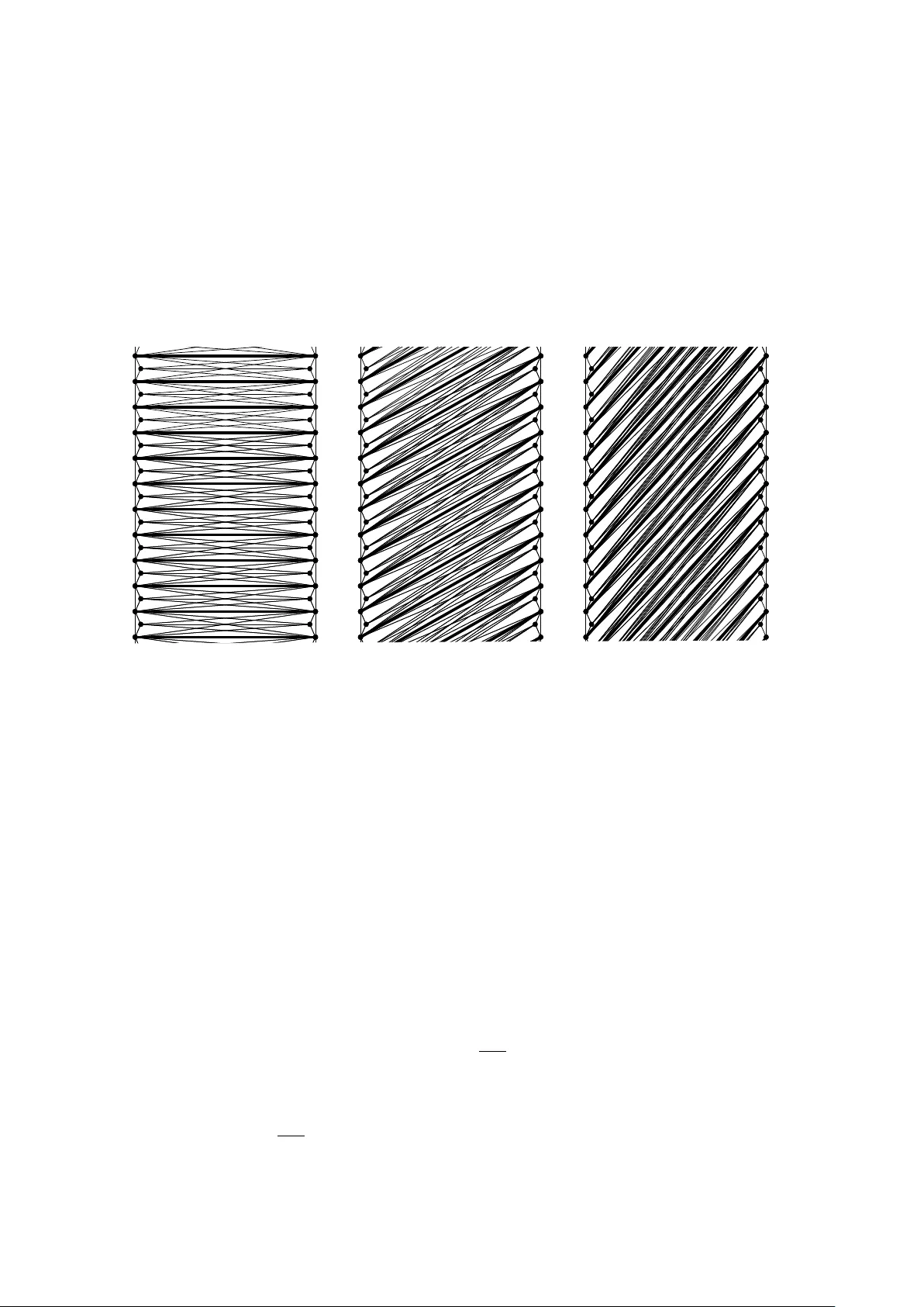
GRAPH BOOTSTRAP PER COLA TION — A DISCO VER Y OF SLO WNESS D A VID F ABIAN, P A TRICK MORRIS 1 , ∗ , AND TIBOR SZAB ´ O 2 , † Abstract. Graph b o otstrap p ercolation is a discrete-time process capturing the spread of a virus on the edges of K n . Giv en an initial set G ⊆ K n of infected edges, the transmission of the virus is gov erned by a ﬁxed graph H : in each round of the pro cess any edge e of K n that is the last uninfected edge in a copy of H in K n gets infected as w ell. Once infected, edges remain infected forever. The pro cess was in troduced by Bollob´ as in 1968 in the context of w eak saturation and has since inspired a v ast array of b eautiful mathematics. The main fo cus of this surv ey is the extremal question of how long the infection pro cess can last b efore stabilising. W e give an exp osition of our recen t systematic study of this maximum running time and the inﬂuence of the infection rule H . The topic turns out to p ossess a wide v ariet y of interesting b eha viour, with connections to additive, extremal and probabilistic com binatorics. Along the w ay we encounter a n umber of surprises and attractiv e open problems. A survey prepared for the o ccasion of the 31 st British Combinatorial Conference (BCC) 2026 Cardiﬀ Universit y , Cardiﬀ, W ales. 1 Dep ar t ament de Ma tem ` atiques, Universit a t Polit ` ecnica de Ca t aluny a (UPC), Barcelona, Sp ain. 2 Institute of Ma thema tics, Freie Universit ¨ at Berlin, Germany E-mail addr esses : dfabian@mailbox.org, pmorrismaths@gmail.com, szabo@math.fu-berlin.de . Date : March 17, 2026. ∗ Researc h supp orted by the DFG W alter Benjamin program - pro ject num b er 504502205, and b y the Europ ean Union’s Horizon Europ e Marie Sk lo do wsk a-Curie grant RAND-COMB-DESIGN - pro ject n umber 101106032 ⋆ ⋆ ⋆ ⋆ ⋆ ⋆ ⋆ ⋆ ⋆ ⋆ ⋆ ⋆ . † Researc h supported b y the DFG under German y’s Excellence Strategy - The Berlin Mathematics Research Cen ter MA TH+ (EXC-2046/1, pro ject ID: 390685689). 1 Contents 1. In tro duction 3 1.1. W eak saturation 3 1.2. P ercolation thresholds 4 1.3. Maxim um running times 4 1.4. The conten t and the goal of this survey 4 1.5. Organisation and notation 4 1.6. What is not included 5 2. Cliques and c hains 6 2.1. W eak saturation for cliques 6 2.2. P ercolation thresholds for cliques 7 2.3. Maxim um running times for cliques 7 3. Pro of highligh t: M K 5 ( n ) low er b ound 11 3.1. The construction 11 3.2. The set of dilations. 12 3.3. Finishing the pro of 14 4. H -p ercolating graphs 15 4.1. Minimal H -p ercolating graphs 16 4.2. H -p ercolating random graphs 17 4.3. Slo w H -p ercolating graphs 17 5. (Almost) quadratic running times 22 5.1. Minim um degree 22 5.2. Random graphs 22 5.3. Constan t av erage degree 23 5.4. Pro of tec hnique: Chain constructions 24 6. Sub-linear running times 26 6.1. T rees 26 6.2. Cycles 27 7. Graph parameters and the running time 28 7.1. The role of the degrees 28 7.2. Pro of tec hnique: Sim ulation 30 7.3. The sub-linear regime 31 7.4. The role of connectivity 32 7.5. A conjecture on tree-width 33 8. Bipartite infection rules 34 8.1. Small graphs 35 8.2. Large complete bipartite graphs 36 9. Disconnected infection rules 37 9.1. F orests and 2-regular graphs 37 9.2. Bounds obtained from simulation 38 9.3. In teracting infection rules 39 References 39 2 1. Introduction The central notion of this survey is gr aph b o otstr ap p er c olation , a term coined b y Balogh, Bollob´ as, and Morris [ 13 ], although the pro cess itself app eared muc h earlier, in a diﬀeren t con text, in w ork of Bollob´ as [ 24 ]. Giv en graphs H and G , let n H ( G ) denote the n um b er of copies of H in G . The H -b o otstr ap p er c olation pr o c ess ( H -pr o c ess for short) on a graph G is the sequence ( G i ) i ≥ 0 of graphs deﬁned b y G 0 := G and for i ≥ 1, V ( G i ) := V ( G ) and E ( G i ) := E ( G i − 1 ) ∪  e ∈  V ( G ) 2  : n H ( G i − 1 + e ) > n H ( G i − 1 )  . Informally , one can imagine a virus spreading in discrete time steps on the edges of the complete graph on V ( G ). Initially just the edges of G are infected. The graph H gov erns the spread of the virus: any edge e of K n whic h is the last uninfected edge in a cop y of H in K n gets infected as w ell. Once infected, edges remain infected forev er. W e call G the starting gr aph and H the infe ction rule of the pro cess. Note that for ﬁnite G , the H -pro cess on G stabilises and we refer to τ H ( G ) := min { t ∈ N : G t = G t +1 } , i.e., the n umber of rounds it takes for that to happ en, as the running time of the H -pro cess on G . W e deﬁne G τ with τ = τ H ( G ) to b e the ﬁnal gr aph of the pro cess, and denote it ⟨ G ⟩ H := G τ . If ev en tually all edges get infected, that is, the ﬁnal graph ⟨ G ⟩ H is the clique K v ( G ) , we say that the starting graph G is H -p er c olating . Example 1.1 (The triangle) . Let H = K 3 and G be an arbitrary n -v ertex graph. Note ﬁrst that no tw o comp onents of G b ecome connected during the K 3 -pro cess as tw o non-adjacent v ertices b ecome adjacen t during a round of the K 3 -pro cess if and only if they hav e a common neigh b our already . Now if x and y are in the same comp onent in G i − 1 then in the next round their distance along a shortest path is reduced to roughly half: dist G i ( x, y ) = ⌈ 1 2 dist G i − 1 ( x, y ) ⌉ . In particular, after ⌈ log 2 (dist G ( x, y )) ⌉ rounds their distance is one and they are adjacen t. Thus w e hav e that τ H ( G ) = max x,y ⌈ log 2 (dist G ( x, y )) ⌉ with the maximum taken o ver pairs of v ertices x, y in the same connected component of G , and ⟨ G ⟩ H is a union of disjoin t cliques on the v ertex sets of the connected comp onents. 1.1. W eak saturation. The graph percolation pro cess w as in troduced b y Bollob´ as [ 24 ] in 1968 for cliques, under the name we ak satur ation , and has since inspired a v ast arra y of b eautiful mathematics. In our terminology , Bollob´ as was in terested in the smallest p ossible num ber of infected edges that p ercolate in the K k -pro cess. Subsequen tly this extremal question turned out to b e greatly inﬂuen tial, as it inspired one of the ﬁrst applications of algebra in extremal com binatorics. F or an arbitrary graph H , wsat( n, H ) denotes the minimum num ber of edges in an H -percolating graph on n v ertices. The concept is motiv ated b y work of Erd˝ os, Ha jnal and Mo on [ 41 ], who determined the smallest num ber of edges on n vertices which K k -p ercolate in a single r ound . Graphs that are H -free and H -p ercolate in one time step are called H -satur ate d . The minimum num ber of edges in an H -saturated graph is denoted b y sat( n, H ), whilst the maxim um n um ber is the T ur´ an numb er ex( n, H ) of H . Clearly wsat( n, H ) ≤ sat( n, H ). Con- sidering Example 1.1 w e see that wsat( n, K 3 ) = sat( n, K 3 ) = n − 1 as an y tree on n vertices p ercolates with a star doing so in one round, whilst any graph with less than n − 1 edges will not p ercolate. 3 1.2. P ercolation thresholds. Whilst weak saturation looks at the smal lest p ossible starting graphs that H -p ercolate, the statistical physics origins of b ootstrap p ercolation motiv ates the in v estigation of r andom initial infection graphs. Balogh, Bollob´ as, and Morris [ 13 ] initiated the study of the threshold probability for when the random graph G ( n, p ) b ecomes H -p ercolating. Here G ( n, p ) denotes the Erd˝ os-R ´ en yi binomial random graph which is obtained b y taking ev ery edge on n vertices indep endently with probability p = p ( n ). W e say an even t holds asymptotically almost surely (a.a.s. for short) in G ( n, p ) if the probabilit y it holds tends to 1 as n tends to inﬁnity . As the prop ert y of b eing H -p ercolating is monotone increasing, the classical result of Bollob´ as and Thomason [ 29 ] gives that there is some threshold p c = p c ( n, H ), suc h that if p = ω ( p c ) then a.a.s. G ( n, p ) is H -p ercolating whilst if p = o ( p c ) then a.a.s. G ( n, p ) is not H -p ercolating. Considering Example 1.1 , w e see that p c ( n, K 3 ) is precisely the threshold for connectivity in G ( n, p ), namely log n/n [ 42 ]. 1.3. Maxim um running times. Another relev an t question concerning p ercolation pro cesses is how long the virus could be spreading for. The study of the corresp onding extremal parameter, concerning the worst case b ehaviour, was sugges ted by Bollob´ as (cf. [ 27 ]). W e deﬁne M H ( n ) := max { τ H ( G ) : G is an n -v ertex graph } , to b e the maximum running time for the H -pro cess on n vertices. Returning to our Example 1.1 , we see that determining M K 3 ( n ) is equiv alent to maximising the distance b etw een tw o v ertices in the same connected comp onen t of an n -v ertex graph G . This is achiev ed when G is a path, giving M K 3 ( n ) = ⌈ log 2 ( n − 1) ⌉ . 1.4. The con ten t and the goal of this survey . In all three settings outlined abov e, inv es- tigations fo cus on understanding how the infection rule H inﬂuences the extremal functions of in terest: the weak saturation num ber wsat( n, H ), the p ercolation threshold p c ( n, H ), or the maxim um running time M H ( n ). The purpose of this surv ey is to explore exactly this, presen ting the current progress and highligh ting the gaps in our knowledge. Indeed, as in all go od math- ematical problems, there are many m ysteries and a full understanding of H -processes presents a formidable challenge. W e will lo ok at b oth weak saturation and p ercolation thresholds in this context and report the foundational w ork as w ell as recent exciting breakthroughs and key unansw ered questions. Ho w ever, this surv ey is mostly concerned with maximum running times. In particular, our pri- mary goal is to give an exp osition of our recent systematic exploration [ 45 – 47 ] of the parameter M H ( n ). W e presen t general pro of metho ds and discov er a rich landscape of theorems with sev eral surprises therein. Along the w ay w e build connections to other topics in extremal graph theory as w ell as probabilistic and additiv e combin atorics. W e in tend this survey to act as an in vitation to the topic, collecting and organising the state of the art and highlighting plen ty of tan talising op en problems and conjectures! 1.5. Organisation and notation. Maximum running times were ﬁrst studied for cliques b y Bollob´ as, Przykucki, Riordan, and Sahasrabudhe [ 27 ] and Matzke [ 66 ], and subsequen tly b y Balogh, Kronen b erg, P okro vskiy , and the third author [ 14 ]. It is these works that w e treat in Section 2 , describing the developmen t of insights that lay the foundation for our results and highligh ting the motiv ations and connections to k ey concepts already present in works on w eak 4 saturation and p ercolation thresholds. In Section 3 we include a no v el concise pro of of a low er b ound of Balogh et al. [ 14 ] on the running time of the K 5 -pro cess. This introduces central facts and deﬁnitions and explains the connection b et w een our problem and additive combinatorics, a link that was ﬁrst utilised in [ 14 ]. In Section 4 we touch on a question that merges the p ersp ectiv e of maxim um running time and percolating graphs. Namely , we prov e that for a broad family of infection rules H , the slo west (up to a constant factor) initial infection conﬁguration can also b e chosen to b e H -p ercolating. In Section 5 we start presenting our results, putting them in con text and introducing key graph properties that contribute to extremely slow running times. Sections 6 and 7 inv estigate what prop ert y of an infection rule causes the process to stabilise quickly for every starting graph. Finally , Sections 8 and 9 are devoted to bipartite and disconnected infection rules, resp ectively . Giv en t w o graphs H and H ′ , the graph H ∩ H ′ denotes the graph on v ertex set V ( H ) ∩ V ( H ′ ) with edge set E ( H ) ∩ E ( H ′ ). The graph H ∪ H ′ is the graph with vertex set V ( H ) ∪ V ( H ′ ) and whose edge set is E ( H ) ∪ E ( H ′ ). The notation H ⊔ H ′ is used to emphasise when the union is a disjoint union , i.e. when V ( H ) ∩ V ( H ′ ) = ∅ . Throughout the surv ey w e will often iden tify graphs with their edge sets. 1.6. What is not included. T o close this introduction, w e brieﬂy mention some highly rel- ev ant directions that are omitted in order to keep this survey (relativ ely) concise. Indeed, there are v ast b odies of work that provide context or study v arian ts to the topics co vered here. Luc kily , there are already fantastic surveys av ailable, by Currie, F audree, F audree and Schmitt [ 37 ] for (weak) saturation, and by Morris for b ootstrap p ercolation [ 67 ] and monotone cellular automata in general [ 68 ]. Neigh b our b o otstrap p ercolation. Besides its intrinsic mathematical interest, graph b o otstrap percolation [ 13 ] was inspired b y the classical notion of r -neighbourho o d b o otstrap p ercolation. There, one initially infects some vertic es of a sp eciﬁc (p ossibly inﬁnite) graph G and at eac h time step, a v ertex b ecomes infected if at least r of its neighbours are infected. This is a monotone cellular automaton (` a la v on Neumann [ 83 ] and Ulam [ 82 ]). The pro cess w as in tro duced by Chalupa, Leath and Reich [ 34 ] on the m -regular inﬁnite tree, as a simpliﬁed mo del of ferromagnets. Subsequently an immense amoun t of literature developed around this concept in combinatorics and probabilit y theory [ 32 , 53 , 54 ] as well as statistical ph ysics [ 1 – 3 ]. Analogously to the graph b o otstrap mo del, there is great interest in when the mo del p er c olates with b oth random starting conﬁgurations [ 10 – 12 , 23 , 33 ] and extremal starting conﬁgurations [ 9 , 12 , 38 , 69 ] b eing studied. Running times of neighbour b o otstrap p ercolation pro cesses hav e recen tly b een addressed from an extremal p ersp ectiv e b y Przykuc ki and Shelton [ 75 ], Przykucki [ 74 ] and Benevides and Przykucki [ 20 , 21 ] and when the starting conﬁguration is random by Bollob´ as, Holmgren, Smith, and Uzzell [ 26 ], Bollob´ as, Smith, and Uzzell [ 28 ] and Balister, Bollob´ as, and Smith [ 8 ]. Hyp ergraphs. The study of weak saturation with resp ect to hypergraphs has b een an imp ortan t topic [ 40 , 72 , 73 , 81 ]. F or the case of threshold probabilities, No el and Morrison [ 70 ] considered a v arian t of the H -pro cess for hypergraphs H where only certain copies of H are activ ated (with some probability), as part of a more general theorem generalising w ork of Kor´ andi, Peled and Sudak o v [ 61 ]. F or maxim um running times, hypergraph cliques H ha v e also b een considered b y No el and Ranganathan [ 71 ], Espun y D ´ ıaz, Janzer, Kronen b erg and Lada 5 [ 44 ] and Hartarsky and Lichev [ 52 ]. Whilst we do not dwell on the topic of hypergraphs for maxim um running times here, we b elieve that it would b e in teresting to explore it further. 2. Cliques and chains W e b egin b y exploring the K k -pro cess for all integers k ≥ 3. 2.1. W eak saturation for cliques. Erd˝ os, Ha jnal and Mo on [ 41 ] pro v ed that for cliques K k with k ≥ 3, one has sat( n, K k ) = ( k − 2)( n − k + 2) +  k − 2 2  =  n 2  −  n − k +2 2  and the unique graph that achiev es this minimum is K k − 2 ∨ ¯ K n − k +2 , the disjoint union of a ( k − 2)-clique and an indep endent set of order ( n − k + 2) with a complete bipartite graph in b etw een. F or k = 3, this matches what we observed in the introduction, and wsat( n, K 3 ) = sat( n, K 3 ) = n − 1. Bollob´ as [ 24 ] prov ed that the weak saturation n um ber and saturation num ber coincide for cliques K k with 3 ≤ k ≤ 7 and later also conjectured [ 25 ] that there is equalit y for all v alues of k . The conjecture was pro v ed by Kalai who gav e t wo pro ofs, one app ealing to the geometric notion of rigidity [ 56 ] and one using exterior algebras [ 57 ]. An elegant pro of inferring it from the Skew Set-Pairs Inequality app ears in a pap er of Alon [ 5 ]. The inequality can b e deriv ed from the pioneering work of Lov´ asz [ 65 ], whic h in troduced the use of exterior algebra in to combinatorics, but was ﬁrst stated and prov ed explicitly by F rankl [ 49 ] (see also [ 5 , 55 ]). Despite the keen interest and m ultiple pro ofs, the determination of wsat( n, K k ) remains one of the intriguing combinatorial problems that to this date do es not ha ve a purely combinatorial solution. One indication for wh y this is the case is the large num b er of non-isomorphic extremal ex- amples. Indeed, unlike the saturation problem, where K k − 2 ∨ ¯ K n − k +2 is the unique graph ac hieving sat( n, K k ) = wsat( n, K k ), when considering K k -p ercolating graphs, as observed al- ready by Bollob´ as [ 24 ], one can build man y more. Indeed, to obtain further constructions one can arbitrarily add a new vertex of degree k − 2 to a K k -p ercolating graph. The following pro- vides a K 4 -p ercolating example with the minimum n um b er of edges, that looks very diﬀerent to K 2 ∨ ¯ K n − 2 . e 1 e 2 e 3 e 4 e 5 Figure 1. A simple K 4 -c hain. Deﬁnition 2.1 (A simple K k -c hain) . Let d ∈ N and n := ( k − 2) d + 2. A simple K k -chain ( H i , e i ) d i =1 of length d is deﬁned as follows. W e tak e H 1 , . . . , H d to b e a sequence of copies of K k suc h that for 1 ≤ i < j ≤ d w e ha ve V ( H i ) ∩ V ( H j ) empty unless j = i + 1, in which case V ( H i ) ∩ V ( H i +1 ) has size tw o and the edge at the intersection is e i . W e let e d b e an edge of H d disjoin t from e d − 1 and w e deﬁne F d to b e the graph obtained b y taking the union ∪ d i =1 H i after remo ving all the edges e i . Note that for an y even n , the graph F d with d = n/ 2 − 1 indeed provides an example of a K 4 -p ercolating graph G with wsat( n, K 4 ) = 2 n − 3 edges. 6 2.2. P ercolation thresholds for cliques. In their pap er in tro ducing the p ercolation thresh- old p c ( n, H ), Balogh, B ollob´ as and Morris [ 13 ] show ed that for cliques of order k ≥ 3 we hav e p c ( n, K k ) = n − 1 /λ ( K k )+ o (1) , (2.1) where λ ( H ) := e H − 2 v H − 2 and the o (1) in the exp onen t is hiding explicit p oly-logarithmic factors in b oth the upp er b ound and low er b ounds. F or a sanit y chec k we note that λ ( K 3 ) = 1, as it should b e to obtain the connectivit y threshold in ( 2.1 ). In order to see where the exp onen t is coming from, consider the simple K k -c hains from Deﬁnition 2.1 . Note that if an edge e ∈ E ( K n ) pla ys the role of e d for some cop y of F d in G ( n, p ) then certainly e will b e infected as one can see that the K k -pro cess on F d infects edge e i at time i for 1 ≤ i ≤ d . No w n − 1 /λ ( K k ) is the threshold for when a ﬁxed edge e ∈ E ( K n ) pla ys the role of a non-edge in a copy of K −− k , the graph obtained from K k b y removing a matc hing of size 2. Indeed, the exp ected num ber of copies of K −− k that ha v e e playing the role of a non-edge is n k − 2 p e ( K −− k ) whic h is constan t at p = n − 1 /λ ( H ) . Therefore, if p is signiﬁcantly ab o v e n − 1 /λ ( H ) (b y some p oly-logarithmic factors, sa y), then any e ∈ E ( K n ) pla ys the role of a non-edge in K −− k , and we can string together these copies to start to build some simple K k -c hain (or rather the resulting graph F d ) in reverse, that has e as its ﬁnal edge e d . There are in fact many wa ys to do this and extending these to length d ≥ log n say , we ﬁnd one in whic h the ﬁnal copy of K −− k added (which will b e the ﬁrst copy in the chain graph F d ) is in fact a copy of K − k (that is, there is an extra edge) and so then we ha v e a chain that causes the edge e to b e infected. With some more care one can apply the second momen t metho d to show that al l edges of K n pla y the role of e d in some cop y of F d in G ( n, p ) and will hence get infected. There is a poly-logarithmic gap b etw een the upp er and low er b ounds in ( 2.1 ). F or K 4 ho w ever, Balogh, Bollob´ as and Morris [ 13 ] could determine p c ( K 4 ) up to a constan t. Subsequen t w ork of Angel and Kolesnik [ 6 ] and Kolesnik [ 60 ] established matching upp er and lo w er b ounds resp ectiv ely , giving a sharp threshold at p c ( K 4 ) = 1 / √ 3 n log n . F or larger cliques, Bartha and Kolesnik [ 15 ] remo v ed the p oly-logarithmic factor from the upp er b ound in ( 2.1 ). In a v ery recen t breakthrough, Bartha, Kolesnik, Kronenberg and P eled [ 17 ] announced the resolution of a sharp threshold for k ≥ 5 at p c ( K k ) = ( γ k n ) − 1 /λ ( K k ) for some explicit constan ts γ k that dep end on F uss-Catalan n umbers. In terestingly there is a change in b ehaviour for k ≥ 5, evidenced by the lack of p oly-logarithmic factors in the threshold. 2.3. Maxim um running times for cliques. As we sa w in the introduction, we hav e that M K 3 ( n ) is logarithmic in n . The situation changes for K 4 . Indeed, it is not diﬃcult to see that the starting graph F d corresp onding to a simple K 4 -c hain in Deﬁnition 2.1 has running time d = n 2 − 1 and so M K 4 ( n ) is at least linear in n . This construction is in fact a bit wasteful. Adding a new vertex to a p ercolating starting graph and connecting it to the endp oints of an edge that only gets infected in the last round, increases the running time by one. (This is in contrast with F d , where the second endp oin t of e i gets the same neighbours as the ﬁrst, hence its addition do es not increase the running time.) Starting with K 4 min us an edge and iterating leads to a construction with running time n − 3. Bollob´ as, Przykuc ki, Riordan and Sahasrabudhe [ 27 ] and, indep endently , Matzke [ 66 ] show ed that this is b est p ossible and M K 4 ( n ) = n − 3, for all n ≥ 3. The upp er bound here adopts the idea of inductively “gro wing” a clique, sho wing that if the pro cess do es not stabilise by step i then there must b e a clique of size i + 3 in G i . 7 F or larger cliques K k , simple c hains again give a linear low er b ound but there is a key diﬀerence with the case of the K 4 -c hain. Indeed, for k ≥ 5 the only edges added in the K 5 - pro cess on F d are the edges e 1 , . . . , e d with e i added in the i th time step. This was not the case for K 4 , where the process on F d p ercolates. The sparse ﬁnal graph of the pro cess on a simple K k -c hain gives hope that a long c hain of copies of K k can somehow be made to wrap bac k onto itself whilst maintaining that each edge e i gets infected at time i . Bollob´ as et al. [ 27 ] and Matzke [ 66 ] b oth managed to do this and achiev e sup er-linear running times. This birthed the concept of a “c hain construction” which has since b een the principal idea for deriving low er b ounds for running times of H -pro cesses. W e therefore introduce the relev ant deﬁnitions in generalit y allowing us to formalise and extend the ideas ab ov e. Moreo v er, chains as deﬁned b elo w also play a c rucial role in deriving upp er b ounds (see Section 5.3.2 ). Deﬁnition 2.2 ( H -c hains) . Let H b e a connected graph, and let τ ≥ 1. An H -chain of length τ is a sequence ( H i , e i ) i ∈ [ τ ] of copies H i of H together with edges e i ∈ E ( H i ) such that e i ∈ E ( H i ) ∩ E ( H i +1 ) for i ∈ [ τ − 1]. W e call G := ∪ τ i =1 H i the underlying gr aph of the H -chain and G ′ := G − { e 1 , . . . , e τ } the starting gr aph of the H -chain. Note that simple K k -c hains are certainly examples of K k -c hains but Deﬁnition 2.2 is muc h more general as there is no restriction on how the copies of H can intersect (other than the edges e i necessarily b elonging to H i and H i +1 ). Our aim is to derive low er b ounds on running times by showing that the edge e i is infected at time i in the K k -pro cess on the starting graph of some K k -c hain. What extra conditions do we need for this? F or the edge e i to get infected at all, we do need some restriction on the in tersections of edge sets of the graphs H i . Also in order that edges e i are not infected to o early in the K k -pro cess, w e w an t that no other edge is infected. Therefore we restrict the copies of K − k , the graph obtained by removing an edge from K k . This leads to the following key lemma. Lemma 2.3 (A lo w er b ound on running times for c hains) . L et k ≥ 5 and τ ≥ 1 and supp ose that ( H i , e i ) i ∈ [ τ ] is a K k -chain such that: ( † ) F or 1 ≤ i < j ≤ τ , we have E ( H i ) ∩ E ( H j ) empty unless j = i + 1 , in which c ase the interse ction is just e i . (*) F or any c opy F of K − k in G := ∪ τ i =1 H i , ther e is an i ∈ [ τ ] such that F ⊆ H i . Then if G ′ := G − { e 1 , . . . , e τ } is the starting gr aph of the chain, we have that τ H ( G ′ ) ≥ τ . Pr o of. Setting G 0 = G ′ to b e the starting graph, w e sho w b y induction that G i = G 0 + { e 1 , . . . , e i } = G i − 1 + e i . The base case i = 0 follows from the deﬁnition. F or i ≥ 1, supp osing that the claim holds for previous i , we hav e that H i − e i ⊆ G i − 1 and so certainly e i is added to G i . T o see that no other edge is added, supp ose an edge f ∈ G i \ G i − 1 completes a copy F ⊆ G i − 1 of K − k to a cop y of K k at time i . As G i − 1 ⊆ G by the induction hypothesis, prop ert y (*) giv es that F ⊆ H j for some j ∈ [ τ ]. As f / ∈ G i − 1 , w e ha v e j ≥ i . If j > i , then H j ∩ G i − 1 = H j − { e j − 1 , e j } b y the induction hypothesis and condition ( † ) . Therefore there are not enough edges in H j ∩ G i − 1 to contain F and so we m ust hav e j = i , F ⊆ H i and f = e i . □ Simple K k -c hains, by construction, satisfy condition ( † ) for every k ≥ 3. It is also easy to see that (*) holds when k ≥ 5. 8 Observ ation 2.4. Suppose that d ∈ N and ( H i , e i ) i ∈ [ d ] is a simple K k -c hain, for some k ≥ 5. If F is some cop y of K − k in G := ∪ i ∈ [ d ] H i , then there is some i ∈ [ d ] such that F ⊆ H i . Indeed, if F w as not contained in an y H i then there w ould b e a choice of e j suc h that remo ving the vertices of e j disconnects F ∼ = K − k , a contradiction. Note that this do es not hold in the case of K 4 . Chains satisfying the hypothesis of Lemma 2.3 are what Bollob´ as, Przykucki, Riordan and Sahasrabudhe [ 27 ] call go o d chains and they used them to give low er b ounds on M K k ( n ) for k ≥ 5. Matzk e [ 66 ] also uses c hains and gav e an explicit construction of a goo d chain showing that M K k ( n ) ≥ Ω( n 3 / 2 ) for all k ≥ 5. Bollob´ as et al. [ 27 ] wen t further, showing that M K k ( n ) ≥ n 2 − 1 λ ( K k ) − o (1) , (2.2) with a random construction. They build their chain by choosing one H i at a time, taking a uniformly random c hoice for the next k − 2 vertices to complete the vertices of H i and then taking e i ∈ H i − e i − 1 also as a random choice. The exp onent in ( 2.2 ) matches that in ( 2.1 ) and this is no coincidence. Indeed, the authors of [ 27 ] show that in terms of un w anted (that is, not con tained in some H i ) copies of graphs F ⊆ K k in G = ∪ i H i , the graph G resembles G ( n, p ) of the same edge density . Therefore if a t ypical edge e ∈ E ( K n ) lies in some (unw an ted) copy of K −− k in G , we can no longer use e as it would create an unw an ted copy of K − k . Th us the pro cess for building the random chain lasts until a t ypical edge is no longer usable. The exponents in ( 2.2 ) tend to 2 as k tends to inﬁnit y , and as sketc hed ab ov e, are optimal with resp ect to a random construction of a go o d chain. Bollob´ as, Przykucki, Riordan and Sahasrabudhe [ 27 ] contemplated that while it is “tempting” to think that their construction is also optimal in general, they had no real reason to believe this. Instead, motiv ated b y the lac k of non-trivial upper bounds in the problem, they opted for conjecturing only M K k ( n ) = o ( n 2 ), that is, that no K k -pro cess should b e able to add a constant fraction of the edges of K n in distinct rounds. Surprisingly , ev en this more mo dest prediction turned out not to hold for k ≥ 6. Balogh, Kronen b erg, P okro vskiy and the third author [ 14 ] gav e an explicit construction of a starting graph with quadratic running time, hence pro ving that M K k ( n ) = Θ( n 2 ) for all k ≥ 6. Theirs w as also a chain construction but with a diﬀerent ﬂav our. In order to get longer running times, in tuitiv ely one needs the chains to intersect more signiﬁcan tly . One key observ ation of [ 14 ] is that the condition ( † ) in Lemma 2.3 can b e substan tially weak ened. Indeed, w e do not really care if distinct H i and H j with j > i + 1 in tersect, as long as the edges e j − 1 , e j are not added b efore they should b e. Thus ( † ) can b e replaced b y ( † ′ ) F or 1 ≤ i < j ≤ τ , w e ha v e e j / ∈ E ( H i ). One can chec k that the pro of of Lemma 2.3 go es through w ith this weak er condition. In [ 14 ] this observ ation was exploited with the construction of a ladder chain whic h w e no w sk etc h for the case of H = K 6 . In fact, the construction we see here is a slight v ariation of the one from [ 14 ] and we instead follo w [ 47 ] whic h generalised the construction to other H (and in tro duced the terminology used here). W e will return to highlight the diﬀerence at the end of the following section after seeing chain constructions in detail. The idea is to sup erimpose linearly many simple c hains on the same vertex set. Each of these simple chain s ( H a i , e a i ) i ∈ [ τ 0 ] will ha ve some linear length, say τ 0 = ⌊ n/ 8 ⌋ . These can then be link ed together via disjoin t simple chains of constan t length to form one long con tinuous chain 9 whic h will hav e quadratic length (w e will see in the next section the details of suc h a linking pro cedure). T o construct the linearly long simple c hains, we start by considering a bipartition of the v ertices into t wo sides which we think of as the left side and a right side. On eac h side we place a sequence of 2 τ 0 copies of K 3 , with consecutiv e copies in tersecting in a singular v ertex. Using these triangles, for any slop e a = 0 , 1 , . . . , τ 0 , we can consider a chain ( H a i , e a i ) i ∈ [ τ 0 ] whic h matc hes the triangle in p osition j on the left to the triangle in position j + a on the right and places a complete bipartite graph b etw een them (see Figure 2 ). W e will take an appropriate collection A of slop es that will deﬁne our family of simple chains. Figure 2. Sections of simple K 6 -c hains with slop es 0 (left), 4 (middle) and 8 (righ t). The edges e i of the simple c hains are b old. Crucial to the analysis of this c hain and establishing the k ey condition (*) of Lemma 2.3 is the fact that the graph G := ∪ a ∈ A,i ∈ [ τ ] H a i induces a sequence of triangles on b oth the left and righ t side. This in turn forces any copy F of K − 6 in G to use three v ertices on the left and three v ertices on the right. Using this, one can show that if F contains edges of the underlying graph ∪ i ∈ [ τ 0 ] H a i for diﬀerent slop es a ∈ A , then t w o of these must hav e diﬀerence at most three. W e can av oid this b y choosing only every fourth integer in to A . In terestingly , the construction do es not work for K 5 . Indeed, the naive generalisation w ould place a sequence of triangles on the left side as before, and a path on the righ t side. F or any p air of simple K 5 -c hains with slop es a  = a ′ using this bipartition, one can ﬁnd copies of K − 5 using one triangle on the left and edges corresp onding to the diﬀerent slop es a, a ′ for the remaining v ertices v , v ′ of the copy . If w e try to include these t w o simple chains as segments of a long c hain, this will lead to unw an ted copies of K − 5 , contradicting (*) . Ho wev er with an alternative, more subtle approach the same authors [ 14 ] achiev ed almost quadratic time: M K 5 ( n ) ≥ n 1 − O (1 / √ log n ) = n 2 − o (1) . In fact their construction giv es that M K 5 ( n ) ≥ n · r 3 ( n ) where r 3 ( n ) is the size of a largest subset of [ n ] free of three-term arithmetic progressions. The famous construction of Behrend [ 19 ] gives that r 3 ( n ) ≥ n 1 − O (1 / √ log n ) , whilst it is w ell-known that r 3 ( n ) = o ( n ), as was originally shown b y Roth [ 76 ] in 1953. 10 W e close this section with what is probably the most pertinent outstanding question in the pursuit of maximum running times, namely determining the asymptotics of M K 5 ( n ). Conjecture 2.5. [Bollob´ as-Przykuc ki-Riordan-Sahasrabudhe [ 27 ]] The maxim um running time for infection rule K 5 is M K 5 ( n ) = o ( n 2 ). 3. Proof highlight: M K 5 ( n ) lowe r bound In this section, we prov e a lo w er b ound for M K 5 ( n ) of the form n 2 − o (1) . This was originally pro v ed by Balogh et al. [ 14 ], using a construction similar to the ladder chains discussed in the previous section, although it uses a tripartition and slopes deﬁned b y Behrend’s set free of arith- metic progressions. Our pro of here uses dilation chains [ 47 ] and is quite distinct, ev en though it also relies on Behrend’s construction. In [ 47 ], w e developed a theory of chain constructions (and in particular the dilation chains which we see here) to give general results that apply to a wide array of infection rules, see for example Section 5.4 . In this section, w e in tro duce the key ideas of c hain constructions and dilation chains in the context of K 5 , where man y technicalities can b e av oided. As with the ladder c hains of the previous section, we will ﬁrst sup erimp ose linearly many simple chains on the same v ertex set, each of linear length. Note that eac h of the chains ( H a i , e a i ) i ∈ [ τ 0 ] there can b e obtained from the chain ( H 0 i , e 0 i ) i ∈ [ τ 0 ] with slop e 0 b y leaving the left side ﬁxed and translating the vertices on the right side by a triangles. The main diﬀerence for dilation c hain constructions will b e the wa y w e choose the p ermutation that “mixes up” the v ertices of a simple chain to obtain other simple chains in our family . The vertex set will b e lab elled b y the elements of Z p \ { 0 } , which is equipp ed with nicely interacting additive and m ultiplicativ e op erations. In the basic simple c hain ( H 1 i , e 1 i ) i ∈ [ τ 0 ] the copies of K 5 s will b e laid out one after the other, following the additive structure of Z p \ { 0 } . The family of simple chains ( H a i , e a i ) i ∈ [ τ 0 ] will b e created using the m ultiplicativ e op eration: the vertices of the basic simple c hain are multiplied by a constan t a ∈ Z p \ { 0 } . W e will again ﬁnd that if we c ho ose the set A of dilation constan ts a appropriately , then there will b e no un w anted copy of K − 5 when w e sup erimp ose the corresp onding simple chains. Let us see this idea formally . 3.1. The construction. Let p ∈ N b e a prime and deﬁne τ 0 := ⌊ p − 3 3 ⌋ . Let A := { a 1 , . . . , a q } ⊆ Z p \ { 0 } b e a subset of q dilations. Dilation chains. F or an element a ∈ Z p \ { 0 } , the dilation K 5 -chain ( H a i , f a i ) i ∈ [ τ 0 ] is deﬁned on the vertex set W = { w i : i ∈ Z p \ { 0 }} such that V ( H a i ) = { w a (3 i − 2) , w a (3 i − 1) , w a (3 i ) , w a (3 i +1) , w a (3 i +2) } (3.1) and f a i = w a (3 i +1) w a (3 i +2) for i = [ τ 0 ]. W e also deﬁne f a 0 = w a w 2 a . The c hain ( H 1 i , f 1 i ) i ∈ [ τ 0 ] is clearly simple and the others are obtained from it by multiplying the indices of the vertices by a . Since p is chosen to b e a prime, the map x 7→ ax is a bijection of Z p \ { 0 } to itself so ( H a i , f a i ) i ∈ [ τ 0 ] is also a simple K 5 -c hain. Linking chains. F or each element a j ∈ A , the dilation c hain ( H a j i , f a j i ) i ∈ [ τ 0 ] will feature as sub chains of our ﬁnal c hain ( H i , e i ) i ∈ [ τ ] . F or ease of notation we use ( H j i , f j i ) i ∈ [ τ 0 ] instead. In order to link these simple c hains up, we in tro duce short simple K 5 -c hains ( L j i , g j i ) i ∈ [3] for j ∈ [ q − 1], each of length 3. The j th linking chain will link the last K 5 of the a j -dilation chain to the ﬁrst K 5 of the a j +1 -dilation c hain. That is, tw o vertices of L j 1 (disjoin t from g j 1 ) will b e 11 the vertices of the edge f j τ 0 and g j 3 will coincide with f j +1 0 , see Figure 3 . All other 7 vertices of U j := ∪ i ∈ [3] V ( L j i ) will b e disjoin t from W and also disjoint from U j ′ \ ( W ∩ U j ′ ) for choices of j ′  = j . W f j τ 0 f j +1 0 Figure 3. A linking K 5 -c hain ( L j i , g j i ) i ∈ [3] with the edges g j i as dashed lines. Note that in order to hav e that ( L j i , g j i ) i ∈ [3] is a w ell-deﬁned simple K 5 -c hain, w e need that f j τ 0 ∈ E ( L j 1 ) and g j 3 = f j +1 0 ∈ E ( L j 3 ) are vertex-disjoin t in W . W e will ensure this when we select the set A of dilations. Bringing ev erything together. Finally , w e deﬁne our c hain ( H i , e i ) i ∈ [ τ ] whic h is simply obtained by concatenating the sequences, starting with ( H 1 i , f 1 i ) i ∈ [ τ 0 ] follo w ed by ( L 1 i , g 1 i ) i ∈ [3] and then ( H 2 i , f 2 i ) i ∈ [ τ 0 ] and so on, alternating b etw een dilation chains and linking chains, until w e ﬁnish with the sequence ( H q i , f q i ) i ∈ [ τ 0 ] . This deﬁnes a K 5 -c hain whic h has length τ := τ 0 q + 3( q − 1) and lies on V = W ∪  ∪ j ∈ [ q − 1] U j  whic h has size | V | = p − 1 + 7( q − 1). 3.2. The set of dilations. In this section, we collect prop erties of the set A that we will need for our dilation c hain construction ab ov e to w ork. First of all, as we promised ab ov e, we make sure that f j τ 0 ∩ f j +1 0 = ∅ for ev ery j ∈ [ q − 1], so the j th linking c hain is simple. F urthermore, in order to use Lemma 2.3 for the running time of ( H i , e i ) i ∈ [ τ ] , we need to establish prop erties (*) and ( † ) for it. Both of these dep end on certain restrictions ab out ho w the edges of diﬀerent dilation chains in teract with each other. At the heart of the pro of of all of these lies a general observ ation, relating the edges of the graph G j := ∪ i ∈ [ τ 0 ] H j i of the j th dilation chain to the existence of a congruence mo dulo p . Observ ation 3.1. If w x w y ∈ E ( G j ) for x, y ∈ [ p − 1] and j ∈ [ q ], then there is some α ∈ Z \ { 0 } with | α | ≤ 4 such that x − y = α a j mo d p. Pr o of. As w x w y ∈ E ( G j ), there is some i ∈ [ τ 0 ] with w x , w y ∈ V ( H j i ) = { w a j (3 i − 2) , . . . , w a j (3 i +2) } . Therefore, there are some distinct ℓ x , ℓ y ∈ {− 2 , − 1 , 0 , 1 , 2 } suc h that x = a j (3 i + ℓ x ) and y = a j (3 i + ℓ y ) mo dulo p . Then x − y = αa j mo dulo p , where α = ℓ x − ℓ y  = 0. □ The prop erties w e need for our main pro of forbid that edges from t wo or three diﬀerent dilation chains form certain small subgraphs in G . The ab ov e observ ation translates these subgraphs to certain linear equations mo dulo p , in at most three v ariables, having a solution from A . This leads us to the next theorem, based on the famous construction of Behrend a v oiding 3-term arithmetic progressions. It gives us large subsets A of Z p whic h do not hav e non-trivial solutions to any of the linear equations we will care ab out. 12 Theorem 3.2 (Behrend [ 19 ]) . Ther e exists C ′ > 0 such that for any prime p ∈ N ther e is some set A ⊂ Z p \ { 0 } such that | A | ≥ p 1 − C ′ / √ log p and if α 1 a 1 + α 2 a 2 + α 3 a 3 = 0 mo d p for some a i ∈ A and α i ∈ Z with | α i | ≤ 4 for i ∈ [3] then P 3 i =1 α i = 0 and a i = a j for al l i, j ∈ [3] with α i , α j  = 0 . Note that in particular, by ﬁxing α 1 = α 2 = 1 and α 3 = − 2, the set A from Theorem 3.2 av oids three-term arithmetic progressions x, x + d, x + 2 d with x, d ∈ Z p and d  = 0. The original pro of of Behrend [ 19 ] simply gav e sets av oiding these arithmetic progressions but it is w ell-kno wn [ 77 , 79 ] that his construction can b e adapted to av oid non-trivial solutions to any constan t num b er of linear equations in at most three v ariables. Distinct dilation c hains are edge-disjoin t. T o guarantee ( † ) we need to make sure that G j and G j ′ do not share an e dge if j  = j ′ . If there was some edge w x w y ∈ G j ∩ G j ′ then b y Observ ation 3.1 w e hav e that there are some α, α ′ ∈ Z \ { 0 } with | α | , | α ′ | ≤ 4 such that αa j − α ′ a j ′ = 0 mo dulo p . This contradicts our choice of A from Theorem 3.2 , since a j , a j ′ ∈ A and a j  = a j ′ . Corollary 3.3. The gr aphs G j with j ∈ [ q ] ar e p airwise e dge-disjoint. Prev en ting “unw an ted” copies of K − 5 . Condition (*) forbids that a copy F of K − 5 in G shares an edge with more than one H i . The most problematic part of showing this turns out to b e if F shares an edge with more than one dilation ch ain. Here is where w e use the full p o wer of the prop erties of our set A from Theorem 3.2 . Lemma 3.4. F or any c opy F of K − 5 in ∪ j ∈ [ q ] G j , ther e is a j ∈ [ q ] with F ⊆ G j . The pro of of this relies on a simple combinatorial observ ation implying that in order to av oid copies of K − 5 that hav e edge from diﬀerent dilation chain s, it is enough to a v oid triangles with that prop erty . F act 3.5. Any non-mono chr omatic e dge-c olouring of K − 5 c ontains a c opy of K 3 , that is non- mono chr omatic. Pr o of of L emma 3.4 . Consider a colouring of ∪ j G j that colours an edge j if it b elongs to G j . If F is not a subgraph of an y of the G j then it is not mono c hromatic and hence there is a triangle F ′ whic h is also not. Let x, y , z ∈ Z p suc h that the vertices of F ′ are w x , w y , w z ∈ W and let j 1 , j 2 , j 3 ∈ [ q ] suc h that w x w y ∈ G j 1 , w x w z ∈ G j 2 and w y w z ∈ G j 3 . By Observ ation 3.1 , w e hav e that for i = 1 , 2 , 3 there are α i ∈ Z \ { 0 } such that | α i | ≤ 4 and x − y = α 1 a j 1 , z − x = α 2 a j 2 and y − z = α 3 a j 3 , mo dulo p . Summing these equations gives that P 3 i =1 α i a i = 0 mo dulo p and th us, as all the α i are non-zero and A satisﬁes the conclusion of Theorem 3.2 , we ha v e that a j 1 = a j 2 = a j 3 , con tradicting that F ′ is non-mono chromatic. □ Linking c hains are simple. Finally , w e also rectify what we left op en at the end of the deﬁnition of linking chains: to ensure that they are simple. Namely , we need to see that for ev ery j ∈ [ q − 1] the edge f j τ 0 and the edge f j +1 0 are disjoint. The vertices of f j +1 0 are w a j +1 and 13 w 2 a j +1 and the v ertices of f j τ 0 are among w a j ( p − α ) , where α ∈ [4]. If tw o of these w ere to coincide then there was α ′ ∈ [2] and α ∈ [4] such that α ′ a j +1 − αa j = 0 mo dulo p , which contradicts the prop ert y of our set A . Corollary 3.6. Every linking chain is simple. 3.3. Finishing the pro of. Finally we show that for appropriate choice of p and A , the K 5 -c hain ( H i , e i ) i ∈ [ τ ] satisﬁes the conditions of Lemma 2.3 , hence the starting graph G ′ := ( ∪ i ∈ [ τ ] H i ) − { e 1 , . . . , e τ } has running time τ = n 2 − o (1) . T o this end, for n ∈ N suﬃciently large, we let p ∈ N be a prime such that n/ 4 ≤ p ≤ n/ 2, whic h exists by Bertrand’s p ostulate/Chebyshev’s theorem, and ﬁx τ 0 := ⌊ p − 3 3 ⌋ as b efore. Let A := { a 1 , . . . , a q } ⊆ Z p \ { 0 } with q ≥ p 1 − C ′ / √ log p for some C ′ > 0 b e the set from Theorem 3.2 . Then for an appropriate C > 0 we ha v e τ := τ 0 q + 3( q − 1) ≥ pq / 4 ≥ n 2 − C / √ log n = n 2 − o (1) . The chains all lie on V = W ∪  ∪ j ∈ [ q − 1] U j  whic h has size | V | = p − 1 + 7( q − 1) ≤ n . W e are left to show conditions (*) and ( † ) of Lemma 2.3 . F or ( † ) note that by construction w e do hav e that E ( H i ) ∩ E ( H i +1 ) = e i for every i ∈ [ τ ]. F or 2 ≤ i + 1 < i ′ ≤ τ we must sho w that E ( H i ) ∩ E ( H i ′ ) = ∅ . Corollary 3.3 applies here unless H i and H i ′ b elong to the same dilation chain or same linking c hain. But these are simple (cf. Corollary 3.6 ) and the prop erty holds by construction. T o establish property (*) w e ﬁx F to b e some cop y of K − 5 in G := ∪ i ∈ [ τ ] H i and sho w that there is some i ∈ [ τ ] suc h that F ⊆ H i . Let us ﬁrst assume that F has a vertex u outside of W , sa y u ∈ U j \ W for some j ∈ [ q − 1]. In case V ( F ) ⊆ U j then we are done by Observ ation 2.4 as G [ U j ] only contains the edges of the j th linking chain which is simple by Corollary 3.6 . Otherwise there is some w ∈ V ( F ) \ U j , which we sho w is imp ossible. On the one hand u and w should hav e at least three common neighbours as they are the non-adjacen t vertices of a cop y of K − 5 in G . This is b ecause all neighbours of u are in U j (and w is not). On the other hand, we claim that their common neigh b ourho o d is contained in one of the b order edges f j τ and f j +1 0 of the j th linking chain, providing a contradiction. Indeed, all U j -neigh b ours of w are in the union f j τ 0 ∪ f j +1 0 , yet u , whose neigh b ourho o d is contained in U j , cannot ha v e neighbours in b oth f j τ 0 and f j +1 0 (since these edges are disjoint by Corollary 3.6 and the linking chain has three copies of K 5 ). Th us w e hav e V ( F ) ⊆ W and hence F ⊆ ∪ j ∈ [ q ] G j . In this case Lemma 3.4 implies that F ⊆ G j for some j ∈ [ q ]. As each dilation chain is simple by construction, Observ ation 2.4 can then b e used to deduce that there is some H i con taining F . □ The idea of the linking c hains which we used for our lo w er bound on M K 5 ( n ) originated in the proof of Balogh et al. [ 14 ] for K 5 . In our recent w ork [ 47 ], w e axiomatised the procedure and giv e general conditions for when chains can b e linked to giv e longer c hains. This reduces the problem of ﬁnding one long c hain to ﬁnding many chain segments, which is often conceptually m uc h easier. Indeed, for example for the ladder chains discussed in Section 2.3 , by using linking c hains one can give the simple c hains with diﬀerent slop es separately and do es not need to w orry about one leading into another. In fact, in their original pro of sho wing that M K k ( n ) is quadratic for k ≥ 6, Balogh et al. [ 14 ] did not use linking chains. Instead, they used unequal sides of the partitions and wrapp ed the triangles around so that each time the chain visits a certain triangle, it do es so with resp ect to a diﬀerent slop e. 14 4. H -percola ting graphs Ha ving explored K k -pro cesses in detail, the rest of the surv ey will be concerned with the inﬂuence of the infection rule H on the H -pro cess, our main fo cus b eing on the running time M H ( n ). Before this, let us brieﬂy take sto ck and recap what we hav e seen in the clique case. In particular, it is interesting to consider the in terplay b et w een the running time of the b o otstrap pro cess and whether or not it percolates. In Section 2 , w e saw that wsat( n, K k ) = sat( n, K k ) and so there are edge-minimal K k -p ercolating starting graphs G that percolate in just one step. The set of extremal constructions for weak saturation is larger though and there are edge-minimal K k -p ercolating graphs which are muc h slow er to p ercolate, for example the simple K 4 -c hains of Deﬁnition 2.1 which take linear time to percolate, asymptotically meeting the slo w est p ossible running time M K 4 ( n ). F or larger k ≥ 5, as noted b y Matzke [ 66 ], the wide class of tight examples for wsat( n, K k ) giv en b y Bollob´ as [ 24 ] using an inductiv e argument, all p ercolate in linear time and so fall far short of the maxim um running time M K k ( n ) which is quadratic (or at least almost quadratic for K 5 ). W e also looked at the threshold p c ( n, K k ) for when a random graph G ( n, p ) is K k -p ercolating. Ab o ve this threshold, w e sa w that typical edges of K n pla y the role of the ﬁnal edge e d of some F d generated by a K k -c hain after remo ving the edges e i . Moreo v er, we can take that this chain is logarithmic in size and so random graphs ab ov e the threshold will also p ercolate fast. In fact, this was studied in detail b y Gunderson, Ko ch and Przykucki [ 51 ] who show ed that just ab o ve the threshold p c ( n, K k ) the random graph will a.a.s. K k -p ercolate in O (log log n ) steps and this time decreases as p increases. On the other hand, the c hain constructions that w e sa w to lo wer b ound M K k ( n ) for k ≥ 5 are far from b eing K k -p ercolating. Indeed, it was crucial to our analysis via Lemma 2.3 that only the edges e i of the chain will b e added during the K k -pro cess. This b egs the question as to whether it is p ossible to hav e a starting graph G such that the K k -pro cess p ercolates but do es so slowly . The main topic of this section is a new result which indicates that it is p ossible for H -p ercolating graphs to be slo w with resp ect to the H -pro cess, even asymptotically achieving the optimal maximal running time M H ( n ). Theorem 4.2 below was noted, but not pro v en, b y Bollob´ as, Przykuc ki, Riordan and Sahasrabudhe [ 27 ] for the case H = K k . Here we show the result for the large class of (2 , 1) -insep ar able infection rules H . Deﬁnition 4.1. A graph H with an edge is called (2 , 1) -sep ar able if it can b e disconnected by deleting at most t w o vertices (and all inciden t edges) and one further edge. Otherwise H is called (2 , 1) -insep ar able . Note that every (2 , 1)-inseparable graph is 3-connected as it has at least ﬁve vertices and cannot b e disconnected by deleting t wo v ertices. F urthermore ev ery 4-connected graph is (2 , 1)- inseparable. Indeed, if the remov al of an edge e and tw o vertices z 1 , z 2 disconnected a 4- connected graph H then so would the remov al of z 1 , z 2 and an appropriate endp oint of e (as H has at least ﬁve vertices). The notion of (2 , 1)-inseparabilit y plays a crucial role with resp ect to c hain constructions. Indeed, it was precisely this property of K 5 that w as used to prov e Observ ation 2.4 sho wing that simple c hains do not induce un w anted copies of K − 5 . Theorem 4.2. F or any (2 , 1) -insep ar able H , ther e is some C = C ( H ) such that for al l n ∈ N , ther e is an H -p er c olating gr aph ˜ G with v ( ˜ G ) ≤ C n and τ H ( ˜ G ) ≥ M H ( n ) . 15 F ollowing [ 27 ], we deﬁne M ′ H ( n ) := max { τ H ( G ) : G is an n -v ertex H -p ercolating graph } . Then clearly one has that M H ( n ) ≥ M ′ H ( n ). Whilst Theorem 4.2 do es not quite give that M H ( n ) = O ( M ′ H ( n )) due to our lack of understanding (see Conjecture 8.9 ) of the functions M H ( n ) and M ′ H ( n ), it do es give a strong indication that this is the case. The (2 , 1)-inseparability is crucial in our proof of Theorem 4.2 as w e adopt ideas from c hain constructions. As w e will see later, there are graphs that are (2 , 1)-separable for whic h we can still use chain constructions, for example the wheel graph or bipartite graphs which satisfy an analogue of inseparabilit y [ 47 ]. F or these, it is lik ely that the proof ideas for Theorem 4.2 can b e extended. F or other graphs H for whic h we know M H ( n ), the constructions for the low er b ounds are often H -p ercolating already . W e therefore conjecture the follo wing. Conjecture 4.3. F or all infection rules H , we ha v e M H ( n ) = Θ( M ′ H ( n )). Before pro ving Theorem 4.2 , we brieﬂy survey what is kno wn about general infection rules H in the context of w eak saturation and p ercolation thresholds. 4.1. Minimal H -p ercolating graphs. Other than H = K k , there are sev eral results that determine wsat( n, H ) exactly . Restricting here to connected H , Borowiec ki and Sidorowicz [ 31 ] noted that wsat( n, C k ) = n − 1 if k is o dd and n when k is ev en. Indeed, any spanning tree will p ercolate if k is o dd and if k is even an extra edge is needed, otherwise the ﬁnal graph will b e complete bipartite. F or trees T , F audree, Gould and Jacobson [ 48 ] sho w ed that wsat( n, T ) do es not depend on n and for an y t -vertex tree, one has t − 2 ≤ wsat( n, T ) ≤  t − 1 2  with b oth b ounds being tigh t for certain trees. F urther w eak saturation n umbers for trees were determined b y Pu and Cui [ 36 ] and recently b y Chen, Liu and Y ang [ 35 ] who show that for any rational α ∈ [1 , 2] there is a family of t -vertex trees whose w eak saturation num bers are of order t α . Also recen tly , Kronenberg, Martins and Morrison [ 62 ] determined wsat( n, K k,k ) and wsat( n, K k,k +1 ) and complete bipartite graphs whose sizes gro w with n were considered in [ 4 ]. Mo ving aw a y from exact results to asymptotics, Alon [ 5 ] prov ed that for every H , there is some constant w H ≥ 0 suc h that wsat( n, H ) = ( w H + o (1)) n . What con trols the constan t w H ? F audree, Gould and Jacobson [ 48 ] established that it is closely related to the minimum degree δ ( H ) of H , showing that δ ( H ) 2 − 1 δ ( H ) + 1 ≤ w H ≤ δ ( H ) − 1 . (4.1) In fact, T erekhov and Zh uk ovskii [ 80 ] found an error in the lo w er b ound whic h they then ﬁxed, as well as showing that every multiple of 1 / ( δ ( H ) + 1) in the interv al is realisable as the limit w H := lim wsat( H ) /n for some graph H . V ery recently Ascoli and He [ 7 ] wen t further, c haracterising all the rationals that are realisable as w H for some H . In terestingly , they show ed that all p ossible rationals at least 3 / 2 are realisable whereas b elo w 3 / 2 the realisable v alues are far more sparse with just one accumulation p oint at 1. They conjecture that all p ossible v alues of w H are rational. W e conclude this section by remarking that there are still many op en questions regarding the b eha viour of wsat( n, H ) and the asso ciated constants w H . In particular, it would b e interesting 16 to determine what prop erties of H control the p osition of w H in the in terv al ( 4.1 ). What ab out for a typical H ? Problem 4.4. What is w H = lim wsat( n,H ) n when H = G ( k , p )? 4.2. H -p ercolating random graphs. With the same pro of as for cliques K k , Balogh, Bol- lob´ as, and Morris [ 13 ] sho w ed an upp er b ound on p c ( n, H ) of the form n − 1 /λ ( H )+ o (1) for b alanc e d infection rules H , where we recall that λ ( H ) := e H − 2 v H − 2 ( 2.1 ) and the o (1)-te rm hides logarithmic factors. Here b alanc e d means that e F − 1 v F − 2 ≤ λ ( H ) for every prop er subgraph F ⊂ H with v F ≥ 3. The balanced condition is necessary due to their use of the second momen t metho d to sho w that t ypical edges lie at the end of simple H -c hains. The authors also show that all cycles C k act lik e K 3 and hav e p c ( n, C k ) coinciding with the connectivit y threshold log n/n . Moreov er, they sho w that the threshold for K 2 , 3 is also p c ( n, K 2 , 3 ) = log n/n which gives an example H where the exponent is not equal to − 1 /λ ( H ). In fact, the pap er also pro vides indication that the general picture is muc h more complex than just what λ ( H ) oﬀers. It is not diﬃcult to see [ 13 ] that the existence threshold for a cop y of H min us an edge in G ( n, p ), namely Ω( n − 1 /λ ′ ) with λ ′ = λ ′ ( H ) = min e ∈ H max F ⊆ H − e e F /v F , pro vides a low er b ound on the H -p ercolation thresh- old for all infection rules H , and it was shown in [ 13 ] that this low er b ound is tigh t when the infection rule H has a p endant edge. They also provide further examples H where the exp onent of the threshold is − 1 λ ′ ( H ) and where it is strictly in b etw een − 1 λ ′ ( H ) and − 1 λ ( H ) . Ba yraktar and Chakrab orty [ 18 ] establish that for the complete bipartite graph K r,s the critical exp onent coincides with the upp er bound − 1 /λ ( K r,s ) of Balogh et al. [ 13 ] when 3 ≤ r ≤ s ≤ ( s − 2) 2 + s , i.e. when K r,s is balanced. F or general H with δ ( H ) ≥ 2 and v ( H ) ≥ 4, Bartha and Kolesnik [ 15 ] prov ed a lo wer b ound n − 1 /λ ∗ ( H )+ o (1) whic h is gov erned b y a more subtle function λ ∗ ( H ) = min e H − e F − 1 v H − v F , where the minim um is taken o ver all subgraphs F ⊂ H with 2 ≤ v F < v H . They show that for balanced graphs λ ∗ = λ , so together with the upp er bound of [ 13 ] the asymptotics of the exp onen t of the threshold is determined for all balanced graphs. Recently Bartha, Kronenberg, and Kolesnik [ 16 ] pro ved H = G ( k , 1 / 2) is balanced a.a.s. and hence the critical exp onent for the H -pro cess p ercolating is equal to − 1 /λ ( H ) for “most” infection rules H . F or non-balanced H , one has that λ ∗ is strictly smaller than λ and may even b e smaller than λ ′ . Therefore, for non-balanced infection rules H , the problem of determining the p ercolation threshold p c ( n, H ) is still an outstanding mystery . The graphs K 2 ,t seem like an in teresting example that is yet to b e understo o d. Indeed, Bidgoli, Mohammadian and T ayfeh-Rezaie [ 22 ] oﬀer both upp er bounds and lo w er bounds on the exponent for p c ( n, K 2 ,t ). F or K 2 , 3 , their upper b ound exp onent had already b e en observ ed to b e tight in [ 13 ]. In [ 22 ] the tightness of their upp er b ound is also established for K 2 , 4 . There the answer is − 10 / 13, which is in terestingly diﬀeren t from − 1 /λ, − 1 /λ ′ and − 1 /λ ∗ . 4.3. Slo w H -p ercolating graphs. In this section, w e pro v e Theorem 4.2 giving H -p ercolating graphs that p ercolate slowly . This pro of has not app eared elsewhere and we b elieve it is of considerable in terest to the communit y . Nonetheless, it is somewhat delicate and a bit of a detour from the main theme of the survey . Therefore the reader may wan t to skip ahead to Section 5 on ﬁrst read. In order to prov e Theorem 4.2 , w e follow a natural strategy . Given n ∈ N , ﬁx a starting graph G that ac hiev es running time τ := M H ( n ) and an edge e τ that is added at time τ in the 17 pro cess on G , the aim is to create a new starting graph ˜ G on O ( n ) v ertices that contains G and do es not in terfere with the H -pro cess on G for the ﬁrst τ steps of the pro cess. The addition of e τ should then trigger the rest of the graph to percolate. In particular, we wan t that for ev ery edge f on V ( G ) that do es not lie in ⟨ G ⟩ H , there is some gadget that is triggered b y e τ and forces f to be infected. A natural candidate for such a gadget is a simple H -chain . Here, as with our simple K k -c hains, a simple H -c hain is just a sequence ( H i , e i ) i ∈ ℓ of copies of H with consecutive copies H i and H i +1 in tersecting in a single edge e i ∈ H i ∩ H i +1 (and no other in tersections b etw een the H i ). As we sa w for H = K 5 in Observ ation 2.4 , we ha v e the follo wing. Observ ation 4.5. If H is (2 , 1)-inseparable and ( H i , e i ) i ∈ ℓ is a simple H -c hain then for an y e ∈ E ( H ) and any copy F of H − e in ∪ i ∈ [ ℓ ] H i , there is some i ∈ [ ℓ ] such that F ⊆ H i . As a consequence of this observ ation, note that if e 0 ∈ H 1 − e 1 the graph G ′ = ∪ ℓ i =1 H i − { e 0 , . . . , e ℓ } is H -stable , that is, no edge is added in the H -pro cess on G ′ . Indeed, for each i ∈ [ ℓ ], w e hav e that V ( H i ) hosts e ( H ) − 2 edges in G ′ and so w e cannot em bed some copy of H − e in to H i . No w armed with these simple H -chains, in a similar fashion to the linking c hains used to lo w er b ound M K 5 ( n ), for each f ∈  V ( G ) 2  − ⟨ G ⟩ H , we can place a short simple c hain ( H i , e i ) i ∈ [ ℓ ] suc h that e τ is some edge of H 1 − e 1 , f = e ℓ and all other vertices of the c hain are disjoin t from V ( G ), with the new vertices in tro duced by these chains being distinct for diﬀerent c hoices of f . One immediate problem with this strategy is that we migh t b e adding to o many v ertices. Indeed, it could b e that there are quadratically many edges f ∈  V ( G ) 2  − ⟨ G ⟩ H and eac h one requires adding constantly man y new vertices. F or this, there is an easy solution. Indeed, w e do not hav e to infect al l of the edges f , just enough of them so as to trigger all edges to b e added even tually . Indeed, as w e saw in Section 4.1 , there is some graph G ′ on n v ertices with ( w H + o (1)) n ≤ v ( H ) n edges that is H -p ercolating. Placing an auxiliary copy of G ′ on V ( G ) and infecting all edges f which lie in G ′ , will b e enough to trigger the process to infect all  V ( G ) 2  edges. There is a second problem which is more serious. Indeed, the ab ov e sketc h sho ws how to infect all of the edges on V ( G ) but in doing so, we added new vertices for our small c hains ( H i , e i ) i ∈ [ ℓ ] used to infect the edges f . There is no guarantee that the edges incident to these new vertices will b e infected by this pro cess. Indeed, the small c hains were chosen to b e vertex- disjoin t from V ( G ) pr e cisely b e c ause we do not wan t the pro cess on the small chains ( H i , e i ) i ∈ [ ℓ ] and the pro cess on G to interact. One w ay to guarantee that vertices gain man y neighbours in the H -pro cess is if they ha v e δ ( H ) − 1 neigh bours in a set that will ev en tually b ecome a large clique, as V ( G ) will b ecome after we ensure that all edges on V ( G ) b ecome infected. Lemma 4.6. L et G b e a gr aph, and U, W ⊆ V ( G ) . If W is a clique of size at le ast v ( H ) − 1 in ⟨ G ⟩ H , and every vertex in U has at le ast δ ( H ) − 1 G -neighb ours in W , then U ∪ W is also a clique in ⟨ G ⟩ H . Pr o of. Let u ∈ U , and let w 1 , . . . , w δ ( H ) − 1 ∈ W b e pairwise distinct G -neigh bours of u . F or w ∈ W \ { w 1 , . . . , w δ ( H ) − 1 } , any map φ : V ( H ) → V ( G ) that sends a v ertex of minimum degree to u , its neigh b ourho o d to { w , w 1 , . . . , w δ ( H ) − 1 } , and the remaining vertices of H to the rest of W is an embedding of H minus an edge into ⟨ G ⟩ H . Thus uw completes a cop y of H and there 18 m ust b e a complete bipartite graph b et w een U and W in ⟨ G ⟩ H . All edges in  U 2  then complete some cop y of H with other vertices c hosen from W and so indeed U ∪ W is a clique in ⟨ G ⟩ H . □ W e will use this to trigger new v ertices to join a clique with V ( G ). Ho w ever, w e cannot add δ ( H ) − 1 edges from every new vertex to V ( G ) without interfering with the H -pro cess on G . W e will be able to do this for some subset U of the new v ertices though. This leads us to consider a new gadget which is similar to a simple H -chain, but has the added prop ert y that if we trigger the infection of a clique on some vertices U in the middle of the chain then the infection will cause the whole gadget to p ercolate. The following lemma details what w e need from this gadget. Lemma 4.7 (The gadget graph) . F or any (2 , 1) -insep ar able H on k vertic es, ther e exists a gr aph Γ on ℓ ≤ k 4 k vertic es to gether with an e dge e ∈ E (Γ) and a non-e dge f ∈  V (Γ) 2  \ E (Γ) such that (1) Γ − e is H -stable (no e dge is adde d in the H -pr o c ess on Γ − e ) and f ∈ E ( ⟨ Γ ⟩ H ) , (2) dist Γ ( e, f ) ≥ k , (3) ther e is U ⊆ V (Γ) such that Γ ∪  U 2  is H -p er c olating and dist Γ ( U, e ∪ f ) ≥ k . Pr o of. Let ℓ := ⌈ 2 k 3 k +3 − 2 k − 2 ⌉ , and let ( H i , e i ) i ∈ [ ℓ ] b e a simple H -c hain of length ℓ . Label the v ertices of the chain b y v 1 , . . . , v r , where r := 2 + ( k − 2) · ℓ ≥ 2 k 3 k +3 , such that the i th cop y of H has v ertex se t { v j : j ∈ [( i − 1) · ( k − 2) + 1 , i · ( k − 2) + 2] } . W rite δ := δ ( H ). Deﬁne Γ by V (Γ) = { v 1 , . . . , v r } and E (Γ) = ∪ ℓ i =1 E ( H i ) \ { e 1 , . . . , e ℓ } ∪ E ′ ∪ E ′′ , where E ′ = n v i v j : i ∈ [ k 3 k ] , j ∈ k 2 · [( i − 1)( δ − 1) + 1 , i ( δ − 1)] o E ′′ = n v r +1 − i v r +1 − j : i ∈ [ k 3 k ] , j ∈ k 2 · [( i − 1)( δ − 1) + 1 , i ( δ − 1)] o , and let e := v 1 v 2 , f := e ℓ , and U := { v i : i ∈ [ k 3 k + 1 , r − k 3 k ] } . T o show (1), note that e i app ears b y step i in the H -pro cess on ∪ ℓ i =1 H i − { e 1 , . . . , e ℓ } and in particular f app ears b y step ℓ . Since ∪ ℓ i =1 H i − { e 1 , . . . , e ℓ } ⊆ Γ w e obtain that f ∈ E ( ⟨ Γ ⟩ H ). T o see that Γ − e is H -stable w e show that there are no copies of H minus an edge in Γ − e . Indeed, if F is suc h a copy then F is not contained in ∪ ℓ i =1 H i − { e, e 1 , . . . , e ℓ } b ecause ( H i , e i ) i ∈ [ ℓ ] is a simple H -chain (as noted after Observ ation 4.5 ). F or this reason at least one edge of F lies in E ′ ∪ E ′′ . Without loss of generalit y w e can assume that E ( F ) ∩ E ′  = ∅ and E ( F ) ∩ E ′′ = ∅ (using here that the largest vertices in an edge of E ′ are of distance greater than k in Γ from the smallest vertices in an edge of E ′′ ). Pic k the largest j ∈ [ r ] such that v j is an endp oin t of an edge e ′ in E ( F ) ∩ E ′ . Note that N k − 1 F − e ′ ( v j ) ⊆ { v i : | i − j | ≤ ( k − 1) 2 } where N k − 1 F − e ′ ( v j ) denotes all the v ertices that can b e reached from v j b y a path in F − e ′ ⊆ Γ − e ′ with at most k − 1 edges. W e used here that any edge e ′′ ∈ E ′ with endp oints v i ′′ , v j ′′ and i ′′ < j ′′ < j must ha ve j ′′ ≤ j − k 2 . Hence there can b e no path b et ween v j and the other endp oint of e ′ in F − e ′ , whic h contradicts the assumption that H is (2 , 1)-inseparable. As to (3), b y construction every v ertex v i with i ≤ k 3 k has at least δ − 1 neighbours in { v i +1 , . . . , v ⌊ r/ 2 ⌋ } , and for i ≥ r − k 3 k + 1, v i is adjacent to at least δ − 1 vertices in { v ⌈ r/ 2 ⌉ , . . . , v i − 1 } . By rep eated applications of Lemma 4.6 , w e see that Γ ∪  U 2  indeed H - p ercolates. Let s := dist Γ ( e, U ) and choose a shortest path v i 1 . . . v i s path from e to U . F or any 19 i ∈ [ k 3 k ] and j ∈ [ r ] with v i v j ∈ E (Γ), w e hav e j ≤ i ( δ − 1) k 2 . Therefore, k 3 k < i s = i 1 · i 2 i 1 · . . . · i s i s − 1 ≤ 2 · ( δ − 1) s − 1 k 2( s − 1) < k 3 s and hence s ≥ k . Similarly , dist Γ ( f , U ) ≥ k . It remains to pro ve (2). As there are no edges b et ween { v 1 , . . . , v k 3 k } and { v r − k 3 k +1 , . . . , v r } , an y path from an endp oint of e to an endp oint of f must use a vertex from U . This implies dist Γ ( e, f ) ≥ dist Γ ( e, U ) ≥ k . □ This puts us in go o d stead but w e still need to ﬁnd a wa y to attac h the set U for each new gadget to δ ( H ) − 1 vertices in V ( G ) without interfering with the pro cess on G . T o do this, we simply add an indep endent set I to G and consider the auxiliary H -p ercolating graph G ′ with linearly man y edges as a graph on v ertex set V ( G ) ∪ I . Therefore our gadgets will force that V ( G ) ∪ I hosts a complete graph and we can attac h the vertex sets U to vertices in I to trigger the p ercolation on the individual gadgets. One more idea is needed to guarantee that the edges b et ween U and I for diﬀerent gadgets do not interact with each other to give unw an ted copies of H min us an edge. W e will use a bipartite graph of large girth to place these edges b et ween gadgets and I , recalling that the girth of a graph is the length of the shortest cycle in the graph. Sp eciﬁcally , we need the following. Lemma 4.8. L et k , d ∈ N b e ﬁxe d. Pr ovide d that n ∈ N is suﬃciently lar ge, ther e exists a bip artite gr aph B with p artite sets X , Y of sizes | X | = n , | Y | = 2 k n such that every vertex in Y has de gr e e d and the girth of B is at le ast k + 1 . Bipartite graphs with many edges and high girth ha v e b een studied thoroughly in the lit- erature, see for example [ 50 , 63 , 64 ]. In fact, w e will use them again in our construction of line chains in Section 7.4 . W e note that for our purp oses we do not require the full strength of those results b ecause the parameters k and d are ﬁxed constants. Indeed, Lemma 4.8 can b e obtained easily b y considering a random bipartite graph with parts X of size n and Y ′ of size (2 k + 1) n , with each edge presen t indep endently with probabilit y p = n − 1+1 / (2 k ) . By an application of Chernoﬀ ’s theorem, a.a.s. all vertices in Y ′ will ha ve degree at least d and by Mark o v’s inequalit y , a.a.s. there will b e at most n cycles of length at most k . Therefore a.a.s. b oth these even ts happ en and we can obtain the graph B in Lemma 4.8 by ﬁrst deleting from Y ′ an y vertex that participates in a cycle of length at most k and then deleting further v ertices of Y ′ and edges to get Y of size exactly k n with each v ertex inciden t to d edges. Finally then, w e give the details of the pro of of Theorem 4.2 Pr o of of The or em 4.2 . Let H b e a (2 , 1)-inseparable k -v ertex graph and G an n -vertex graph with running time τ H ( G ) = M H ( n ). W e construct a sup er-graph ˜ G ⊇ G such that τ H ( ˜ G ) ≥ τ H ( G ) and ˜ G is H -percolating. Introduce an indep endent set I of n new v ertices, and let G ′ b e an auxiliary graph with v ertex set V ( G ) ∪ I such that | E ( G ′ ) | ≤ 2 k n and ⟨ G ′ ⟩ H = K 2 n . Let Γ b e the graph from Lemma 4.7 with ℓ := v (Γ) vertices, and for each f ∈ G ∗ := G ′ \ ⟨ G ⟩ H in tro duce a set W f of ℓ − 4 new v ertices. Fix an edge e τ ∈ G τ \ G τ − 1 and place a copy Γ f of Γ on W f ∪ e τ ∪ f such that for some subset U f ⊆ W f , (1)–(3) of Lemma 4.7 hold for e τ , f , U f (with e τ pla ying the role of e ). Consider an auxiliary bipartite graph B b etw een I and { U f : f ∈ G ∗ } such that (i) deg B ( U f ) = d := | U f | · ( δ ( H ) − 1) for all f ∈ G ∗ , 20 (ii) B has girth at least k + 1. Suc h an auxiliary graph exists by Lemma 4.8 whenever n is suﬃciently large, deleting arbitrary v ertices from the set Y to get a set of size e ( G ∗ ), if necessary . F or eac h f ∈ G ∗ c ho ose a partition N B ( U f ) = ∪ u ∈ U f N u in to | U f | sets of size δ ( H ) − 1. Deﬁne ˜ G by V ( ˜ G ) = V ( G ) ∪ I ∪  ∪ f ∈ G ∗ W f  , E ( ˜ G ) = E ( G ) ∪  ∪ f ∈ G ∗  E (Γ f − e τ ) ∪ { v u : u ∈ U f , v ∈ N u }  . With the ab ov e choices there is an edge in the auxiliary graph B b etw een v ∈ I and U f whenev er v has a ˜ G -neigh b our in U f . Note also that ˜ G has v ( ˜ G ) ≤ 2 n + 2 k n ( ℓ − 4) ≤ 4 k 4 k n v ertices, as required. First w e show that ˜ G p ercolates. W e hav e G τ ⊆ ˜ G τ since G ⊆ ˜ G . F or each f ∈ G ∗ , Γ f ⊆ ˜ G τ and hence ⟨ Γ f ⟩ H ⊆ ⟨ ˜ G ⟩ H . In particular, f ∈ E ( ⟨ ˜ G ⟩ H ). Therefore, G ′ ⊆ ⟨ ˜ G ⟩ H . Recall that G ′ is H -percolating and so V ( G ′ ) = I ∪ V ( G ) is a clique in ⟨ ˜ G ⟩ H . Every v ertex in ∪ f ∈ G ∗ U f has δ ( H ) − 1 ˜ G -neigh b ours in V ( G ′ ), so V ( G ′ ) ∪  ∪ f ∈ G ∗ U f  is a clique in ⟨ ˜ G ⟩ H b y Lemma 4.6 . Since Γ f ∪  U f 2  p ercolates, V (Γ f ) is a clique in ⟨ ˜ G ⟩ H . Each of the sets V (Γ f ), f ∈ G ∗ , intersects V ( G ′ ) ∪  ∪ f ∈ G ∗ U f  in at least δ ( H ) − 1 vertices. Therefore, rep eated applications of Lemma 4.6 guarantee that ⟨ ˜ G ⟩ H is a complete graph. Finally , w e pro v e that τ H ( ˜ G ) ≥ τ . W e show b y induction that for all 0 ≤ t ≤ τ E ( ˜ G t ) = E ( G t ) ∪ ( E ( ˜ G ) \ E ( G )) . F or t = 0, this simply holds by deﬁnition. F or larger t , supp ose that we hav e prov ed the induction h yp othesis up to step t − 1. This means that the only edges that hav e b een added are the edges in the H -pro cess on G up to time t − 1. In particular, the neigh b ourho o d of any v ertex v ∈ I in ˜ G t − 1 is the same as its neighbourho o d in ˜ G . Let F b e a cop y of H minus an edge in ˜ G t − 1 . Supp ose ﬁrst that V ( F ) in tersects I . As N ˜ G t − 1 ( v ) = N ˜ G ( v ) ⊆ ∪ f ∈ G ∗ U f , the connectedness of F and the inequalit y dist Γ f ( e τ ∪ f , U f ) ≥ k imply that V ( F ) ⊆ I ∪  ∪ f ∈ G ∗ W f  . Every v ∈ V ( F ) ∩ I has at most one F -neighbour in U f for eac h f ∈ G ∗ , and hence |{ f ∈ G ∗ : U f ∩ N F ( v )  = ∅ }| ≥ δ ( F ) > 2, using that H is (2 , 1)- inseparable in the last inequalit y here. Moreo v er, for ev ery f ∈ G ∗ suc h that U f ∩ V ( F )  = ∅ , w e m ust hav e that there are at least tw o B -neigh b ours of U f in I as otherwise w e could disconnect F b y removing one vertex, con tradicting the (2 , 1)-inseparability of H . Therefore we ha v e that B [( I ∩ V ( F )) ∪ { U f : U f ∩ V ( F )  = ∅ } ] has minimum degree greater than t w o and therefore con tains a cycle. Each vertex in this cycle corresp onds to (at least one) vertex of V ( F ) and these v ertices are distinct. Hence the cycle has length at most v ( F ) = k which contradicts the assumption that the girth of B is at least k + 1. W e hav e shown that I ∩ V ( F ) = ∅ , or equiv alently , V ( F ) ⊆ V ( G ) ∪  ∪ f ∈ G ∗ W f  . If V ( F ) ∩ W f  = ∅ for some f ∈ G ∗ and V ( F ) ⊆ V (Γ f ) then either f ∩ V ( F ) or e τ ∩ V ( F ) is a vertex-cut of H ′ b ecause dist Γ f ( e τ , f ) ≥ k . This, how ev er, w ould con tradict the assumption that H is (2 , 1)-inseparable. Consequen tly , V ( F ) ⊆ V ( G ) and F ⊆ G t − 1 b y the induction hypothesis. Therefore any edge that is added during the step t of the F -process on ˜ G b elongs to G t \ G t − 1 and we are done. □ 21 W e remark that the constan t C = C ( H ) app earing in Theorem 4.2 is probably unnecessary and a similar result should be achiev able with a new starting graph ˜ G on (1 + o (1)) n vertices. An approac h to do this by packing gadgets onto o ( n ) vertices using a high girth (approximate) design w as suggested b y the anon ymous referee. W e did not pursue this direction, but we b elieve that it should indeed b e p ossible. 5. (Almost) quadra tic running times In this section, we begin our exploration of M H ( n ) for general infection rules H . Our ﬁrst p oin t of in terest will b e to what extent the b ehaviour of large cliques (of size at least ﬁv e) generalises to other infection rules H . The results of this section are from our pap er [ 47 ] and are ac hieved through a program of building a general framew ork for chain constructions, in particular exploiting the ideas b ehind the ladder c hains and dilation chains that we already encoun tered. This metho d turns out to b e ﬂexible and we are able to show extremely slo w, that is (almost) quadratic, running times for a large arra y of infection rules H , including many that are far from resem bling the large cliques that we set out to generalise. F or one of our almost quadratic examples, namely the wheel graph, we are also able to complemen t our low er b ound with a non-trivial sub-quadratic upp er b ound. This establishes a new b ehaviour for maxim um running times, exactly the type Conjecture 2.5 predicts for K 5 . 5.1. Minim um degree. In our ﬁrst generalisation of the results of Balogh et al. [ 14 ] for cliques, w e establish Dirac-type conditions for quadratic and almost quadratic running times. Theorem 5.1 ([ 47 ]) . Supp ose 5 ≤ k ∈ N and H is a gr aph with v ( H ) = k . We have that M H ( n ) ≥ ( Ω( n 2 ) if k ≥ 6 and δ ( H ) > 3 k / 4 ; (5.1) n 2 − O (1 / √ log n ) = n 2 − o (1) if δ ( H ) ≥ k / 2 + 1 . (5.2) These tw o b ounds extend the results of [ 14 ] for K k , k ≥ 6 and for K 5 , resp ectively , to arbitrary infection rules that are dense enough in terms of their minimum degree. Later w e will see examples of graphs with minimum degree k / 2 and running time p olynomially separated from quadratic, so the second minim um degree condition is optimal. In fact, as we will see, Theorem 5.1 is b est p ossible not only in guaran teeing almost quadratic running time, but ev en just sup er-linear. A question that remains op en is to fully understand the b ehaviour of quadratic maximum running time in terms of the minim um degree. Problem 5.2. Determine the smallest constan t c min > 0, such that any infection rule H with v ( H ) = k suﬃciently large and δ ( H ) > c min k has M H ( n ) = Θ( n 2 ). In particular is there a graph H with δ ( H ) ≥ k / 2 + 1 that exhibits a sub-quadratic running time M H ( n ) = o ( n 2 )? 5.2. Random graphs. Theorem 5.1 already establishes that cliques of size at least 5 are far from unique in ha ving maxim um running time that is (almost) quadratic. Our next result sho ws that in fact almost al l infection rules on n vertices hav e quadratic running time. In fact, unlike Theorem 5.1 , where the density is a large constant, for typical infection rules H , a very sparse densit y turns out to b e suﬃcien t to cause quadratic b eha viour. 22 Theorem 5.3 ([ 47 ]) . L et H = G ( k , p ) . Then with pr ob ability tending to 1 as k → ∞ we have that M H ( n ) = ( O (1) if p ≤  1 2 − o (1)  log k /k ; (5.3) Ω( n 2 ) if p = ω (log k /k ) . (5.4) Theorem 5.3 shows a stark phase transition in the b ehaviour of H = G ( k , p ) around the connectivit y threshold log k /k . W e remark that M H ( n ) is not necessarily monotone with resp ect to H and so there is no reason, a priori, to exp ect suc h a threshold t yp e result for H = G ( k , p ). It is natural to ask whether this threshold is sharp er than presented here. The 0-statemen t, asserting that M H ( n ) is constan t when p is small, follo ws from the fact that an isolated edge o ccurs a.a.s. (see for example [ 30 , Theorem 5.4]). The 1-statement, giving quadratic running time for p muc h larger than log k /k , is more delicate an d in particular, w e use that H = G ( k , p ) is self-stable, i.e. the H -process is stabilises on H as the starting graph. F or this we apply a result of Kim, Sudak o v and V u [ 59 ]. Whilst it is believ able that results on the asymmetry of G ( k , p ) can b e strengthened to give that H = G ( k , p ) is a.a.s. self-stable as so on as p > log k /k , we did not ﬁnd suc h a result in the literature and it is not immediate ho w one could pro ve suc h a statemen t. Nonetheless, we b elieve it is lik ely that our pro of can be pushed to give M H ( n ) = Ω( n 2 ) a.a.s. already when p > c 1 log k /k for an y c 1 > 1. The range log k / 2 k < p < log k /k seems to b e the most interesting and it is unclear what to exp ect for the b ehaviour of M H ( n ) with H = G ( k , p ). Problem 5.4. Determine the t ypical b ehaviour of M H ( n ) for the random infection rule H = G ( k , p ) in the range  1 2 + o (1)  log k k < p = O (log k/k ). With the additional condition p < log k k , the infection rule H in the problem will a.a.s. hav e one gian t comp onen t and some isolated vertices, which can b e ignored from the p ersp ective of running times. There will also b e v ertices of degree one which suggests that our c hain constructions will be useless for pro ving low er b ounds on M H ( n ) as copies of H minus an edge will b e abundan t and so no analogue of the key prop ert y (*) from Lemma 2.3 can hold. Con v ersely , as w e will see in Section 7.1 , the existence of degree 1 vertices alone is not enough to b e able to prov e eﬀective upp er b ounds on running times. It w ould also b e very interesting to determine the typical b eha viour of M H ( n ) for H b eing a random d -regular graph, which we exp ect to b e (almost) quadratic even for d ≥ 3. Suc h results w ould also b e helpful to b e com bined with the metho ds of Section 7 to generate interesting no v el b eha viours. 5.3. Constan t a v erage degree. The in tuitiv e rule of th um b for the possibility of slo w running time is that the infection rule H is dense. The rationale b ehind this is that dense graphs in c hains are easier to hide from interfering with other chains due to their complex in ternal structure, while sparse graphs ha ve m uch less such connections. Theorem 5.3 ab out the random graph H = G ( k , p ) already indicates the limitations of this intuition, sho wing that a super-logarithmic a v erage degree is enough for a typical infection rule H to hav e a slow running time. Our next results go further, identifying t w o very sparse explicit families with almost quadratic running time. 5.3.1. The squar e of the Hamilton cycle. The ﬁrst result is ab out the 4-regular family of the squar es of Hamilton cycles . T o construct the square of the Hamilton cycle one orders the k v ertices cyclically and connects any tw o of them whose distance is at most tw o. 23 Theorem 5.5 ([ 47 ]) . If H with k ≥ 5 vertic es c ontains the squar e of a Hamilton cycle, then M H ( n ) ≥ n 2 − O (1 / √ log n ) = n 2 − o (1) . Note that Theorem 5.5 also generalises the result on K 5 of Balogh et al. [ 14 ] as the square of a cycle of length 5 is K 5 . The fact that the result only requires that the infection rule c ontains something is notew orthy . As we will see in Section 7 the function M H ( n ) is v ery far from b eing monotone in the infection rule H . 5.3.2. The whe el. Our second result establishes an almost quadratic low er b ound for the maxi- m um running time of a sequence of graphs with av erage degree strictly less than four. The whe el gr aph W k is deﬁned to b e the graph with k + 1 vertices obtained b y taking a cycle of length k and adding a new v ertex that is adjacen t to all vertices of the cycle. The striking feature of this example is that w e can also couple the low er b ound with a non-trivial upper b ound. In particular this in tro duces a completely new b eha viour of p ossible maximum running times, whic h is sub-quadratic but larger than an y polynomial of degree smaller than 2. This can b e seen as evidence for the v alidit y of Conjecture 2.5 which predicts a similar b eha viour for K 5 . Theorem 5.6 ([ 47 ]) . L et k ≥ 7 b e an o dd inte ger. The whe el gr aph W k satisﬁes M W k ( n ) ≥ n 2 − o (1) and M W k ( n ) = o ( n 2 ) . In general, upp er bounds on M H ( n ) are hard to come b y an d require pro ving that the process stabilises in a b ounded num b er of rounds no matter which n -vertex starting graph G 0 is giv en. One k ey idea in our pro of is that c hains ( H i , e i ) i ∈ [ τ ] , whic h are incredibly useful for lo w er bounds (see Section 5.4 b elo w), can also b e used for upper bounds! Indeed, when pro ving upp er bounds, w e hav e very little information about the graphs G i in the pro cess whose running time we are trying to b ound. How ev er in any H -pro cess ( G i ) i ≥ 0 with running time τ := τ H ( G 0 ) we can em b ed an H -chain ( H i , e i ) i ∈ [ τ ] . Indeed, starting with some edge e τ added at time τ there is a cop y H τ of H completed b y e τ . The edge e τ − 1 is then chosen as an edge of H τ that is added at time τ − 1, which m ust exist as otherwise e τ w ould b e added before time τ . Deﬁning H τ − 1 to b e a cop y of H completed by e τ − 1 and contin uing this pro cess, we can deﬁne the full chain ( H i , e i ) i ∈ [ τ ] . Although the starting graph of this chain may not b e G 0 , or even con tained in G 0 , the chain still gives us some concrete structure in whic h to work on for upp er b ounds. Another in teresting feature of our proof of the upp er b ound in Theorem 5.6 is that w e use the famous R uzsa-Szemer´ edi (6 , 3) -pr oblem/the or em [ 78 ] which states that any n -vertex 3-uniform h yp ergraph with no 6 v ertices inducing 3 or more edges, must hav e o ( n 2 ) edges. 5.4. Pro of technique: Chain constructions. All of the low er b ounds stated ab o ve as w ell as several further results later in the survey follo w from v arious chain constructions. Part of the c hallenge for applying chain constructions to infection rules H that are not complete is to ﬁnd the “correct” w a y to generalise deﬁnitions and prop erties. In [ 47 ], we axiomatised the pro cedure, giving weak conditions on H -chains ( H i , e i ) i ∈ [ τ ] that allow us to con trol the running time of the pro cess based on a c hain. The resulting notion of pr op er c hains is somewhat tec hnical. Suﬃce it to sa y here that we deriv e an analogue to Lemma 2.3 whic h giv es lo w er bounds on running times for prop er c hains, with the key prop erty b eing analogous to the condition (*) asking to a v oid “un w anted” copies F of H minus an edge, that span several H i . W e also placed the linking c hains that we sa w for K 5 in to this general framework, which allo w ed us to simply exhibit some 24 collection H of simple H -chains which satisﬁes the notion of prop erness. In particular, we need to a void “lo cal” unw an ted copies F of H minus an edge, that is, those that are induced b y one segmen t c hain ( H a i , e a i ) i ∈ [ τ 0 ] in the collection H but do not lie in a single V ( H i ), and “crossing” copies F of H minus an edge, that span the edges of sev eral diﬀeren t chains in H . Av oiding local copies F of H − e for some edge e ∈ H essentially b oils down to sho wing that w e cannot place such a copy F on the edges of a simple H -c hain ( H i , e i ) i ∈ [ τ 0 ] without placing it on V ( H i ) for some i ∈ [ τ 0 ]. F or H = K 5 , we noticed this via Observ ation 2.4 . F or general infection rules H , there is no guarantee that w e cannot separate a cop y F of H − e across a vertex cut of size 2 (giv en by some edge e i of the chain). This motiv ates the deﬁnition of (2 , 1)-inseparability from Section 4 , whic h provides a simple condition on H that suﬃces to a v oid the lo cal unw an ted copies of H − e . As with K 5 , in many cases w e can forbid the presence of crossing unw an ted copies F of H − e b y placing dilation chains H according to an appropriate dilation set A which a voids solutions to certain linear equations and placing one simple H -chain corresp onding to each dilation. Through F act 3.5 , we show ed that an unw an ted copy of K − 5 leads to a triangle s panning more than one chain. In some of our applications in this section, for example for the wheel graph W k , we cannot guarantee this. W e can how ev er work with a slightly weak er concept. Deﬁnition 5.7. A graph F is called Behr endian if for an y non-mono chromatic colouring of the edges in F there is a non-mono c hromatic cycle C ⊆ F whic h is the union of t w o or three mono c hromatic paths. The non-mono chromatic cycles from Deﬁnition 5.7 can still be a v oided by taking a dilation set A whic h is of Behrend type, as in Theorem 3.2 , and choosing the constant b ounding the size of the co eﬃcients of the equations to b e suﬃcien tly large in terms of k = v ( H ). W e therefore arriv e at the follo wing theorem. Theorem 5.8 ([ 47 ]) . L et H b e a (2 , 1) -insep ar able gr aph such that H − e is Behr endian for every e ∈ H . Then M H ( n ) ≥ n 2 − o (1) . Theorem 5.5 and the second part of Theorem 5.2 are corollaries although chec king b oth the (2 , 1)-inseparabilit y and Behrendian prop erty is not immediate. The wheel do es not follow from Theorem 5.8 as it is (2 , 1)-separable. Indeed, it has v ertices of degree three that can b e disconnected from the rest of the graph b y removing an inciden t edge and the t w o other adjacent v ertices. Nonetheless, we can apply our mac hinery by explicitly building simple W k -c hains that a v oid lo cal unw an ted copies of the wheel minus an edge. F or the quadratic low er b ounds given in this section, w e use ladder chains similar to those used for K 6 , see Figure 2 . W e split the vertex set V ( H ) into L ∪ R , place a sequence of copies of H [ L ] on the left with consecutiv e copies in tersecting in a single v ertex and similarly on the righ t. Each simple H -chain ( H a i , e a i ) i ∈ [ τ ] in our collection will then b e placed with H i c ho osing a cop y of H [ L ] from the left and a copy of H [ R ] according to some slop e a . F or K 6 , b oth H [ L ] and H [ R ] w ere simply copies of K 3 and this greatly simpliﬁes the analysis of this construction. Indeed, it is not hard to show that any unw an ted copy of K − 6 will ha ve to use one of the triangles on the left and one on the righ t. T o do this for our applications of dense graphs and random graphs is considerably more intricate. Indeed, for the dense graphs w e ha ve v ery little 25 information ab out the structure of H and the random graphs H = G ( k, p ) that we treat can b e v ery sparse. F or the ﬁrst part of Theorem 5.2 , as with Theorem 5.8 ab ov e, we actually deriv e a more general theorem. W e say that a graph H is ( ℓ, 1) -insep ar able if it cannot b e disconnected by the remov al of an edge and at most ℓ vertices. Theorem 5.9 ([ 47 ]) . If H is ( ⌈ v ( H ) / 2 ⌉ , 1) -insep ar able, then M H ( n ) = Ω( n 2 ) . F urther natural examples of k -vertex ( ⌈ k / 2 ⌉ , 1)-inseparable graphs are complete tripartite graphs with no part larger than ⌊ k / 2 ⌋ − 2 and t th p o wers of cycles for t ≥ k / 4 + 1, whic h are obtained by cyclically ordering the v ertices and connecting eac h v ertex to all v ertices within distance t in the ordering. 6. Sub-linear running times After seeing infection rules with long running times, we now jump to the other end of the sp ectrum and explore infection rules for which the pro cess stabilises fast. 6.1. T rees. W e b egin with an example. Example 6.1. F or the path P t with t ≥ 2 vertices, M P t ( n ) ≤ 3. Pr o of. If t = 2, ev ery edge of K n is infected immediately , so M P 2 ( n ) = M K 2 ( n ) = 1. More generally , unless the starting graph is P t -stable, the ﬁrst round creates a copy P of P t . In the second round, b oth leav es of P b ecome adjacen t to ev ery other vertex (including vertices of P ). Moreo v er, as at this p oint every vertex in V ( G 0 ) is a leaf of a cop y of P t , in the third round all these vertices also b ecome univ ersal and the pro cess terminates with K n . □ Infection rules H with a p endant v ertex seem to spread the virus very fast: Any vertex in a cop y of H with a p endan t neigh b our in H will b ecome almost univ ersal, that is, connected to ev ery vertex outside the cop y of H , in the next round. In particular in every tree T -pro cess, after just the second round every leaf-neighbour within any copy of T created in the ﬁrst round is already almost univ ersal. Do es this mean that there is an absolute constant that bounds the maximum running time for ev ery tree? This is not quite true; one can witness this with the tree having just a single leaf-neigh b our: the star. Example 6.2. Let T = K 1 ,t − 1 b e the t -vertex star. Then M T ( n ) = t − 1 for all n suﬃciently large. Pr o of. Let us ﬁrst see that if a T -pro cess go es on for t − 2 rounds then it stabilises in the next round. Observ e that the cen tre vertex c i of a copy of K 1 ,t − 1 created in the i th round for some i ≤ t − 2, b ecomes universal at round i . This means that after round t − 2 every vertex has at least t − 2 neigh b ours. So all non-universal v ertices are now centres of K 1 ,t − 1 with one edge missing, and in the next round all v ertices b ecome univ ersal and the T -pro cess stabilises b y p ercolating. F or the low er b ound let us take G 0 to b e the disjoint union of the stars K 1 ,s with cen tre c i , 1 ≤ s ≤ t − 2 and a set W of n −  t 2  + 1 isolated vertices. W e aim to show that the T -process ( G i ) i ≥ 0 on G runs for t − 1 steps b efore stabilising, that is, at least one edge is infected in round 26 t − 1 (and not b efore). W e can see b y induction that for 1 ≤ i ≤ t − 3, the graph G i after round i is the union of the starting graph G 0 and all incident e dges to the i vertices c t − i − 1 , . . . , c t − 2 . Therefore in G t − 3 the v ertices of W are still independent and hav e degree t − 3. V ertex c 1 b ecomes universal in round t − 2, raising the degree of the vertices in W to t − 2. Then in round t − 1 all edges within W will get infected. That means the pro cess did not stabilise b efore round t − 1, so τ H ( G 0 ) ≥ t − 1, as desired. □ This example shows that, unlik e for the case of paths, the maximum running time do es dep end on the size of the star. Nev ertheless it does not dep end on the order n of the starting graph and this is what turns out to extend to any tree T . Our upp er b ound giv es a quadratic dep endence on the num b er of vertices of T . Theorem 6.3 ([ 46 ]) . L et t ∈ N and n ≥ 2 t . Every tr e e T on t vertic es satisﬁes M T ( n ) ≤ 1 8 · ( t 2 + 6 t + 68) . As discussed ab o ve, a neigh b our of a leaf in a copy of the target tree T in G 1 b ecomes an almost univ ersal v ertex during the second round, and hence the diameter of G 2 already becomes constan t, so the statement of Theorem 6.3 perhaps do es not come across as unexp ected. The actual pro of how ev er, that from constant diameter the percolation pro cess ﬁnishes in constant time, turned out to b e a considerable c hallenge. Indeed, the analysis needed to handle all the great v ariet y of trees and choices of starting graph is quite delicate. Moreov er, extra ideas w ere needed to ac hiev e an upp er b ound whose dep endence on t is p olynomial. An in teresting question is to in v estigate ho w tight the upp er b ound of Theorem 6.3 is. Problem 6.4 ([ 46 ]) . F or t ∈ N , determine M ∗ ( t ) := max { lim sup n →∞ M T ( n ) : T is a t -vertex tree } . W e a v oid simply taking a maximum here as it ma y b e that small v alues of n in terfere with the asymptotics and we take the lim sup instead of a limit as w e cannot rule out the p ossibilit y that M T ( n ) oscillates with n . With this notation, Theorem 6.3 gives that M ∗ ( t ) = O ( t 2 ) and stars (Example 6.2 ) giv e M ∗ ( t ) ≥ t − 1. W e exp ect that stars giv e the longest maxim um running time. Conjecture 6.5 ([ 46 ]) . F or all t ∈ N , we hav e M ∗ ( t ) = t − 1. 6.2. Cycles. As discussed in the in tro duction, the K 3 -pro cess alw ays ﬁnishes in at most ⌈ log 2 ( n − 1) ⌉ rounds, and taking the path P n to b e the starting graph realises this. This is still a quite fast infection spread, but not constant anymore. With the pro of of this in mind it should b e of no great surprise that the maximum running time of the C k -pro cess for an y cycle length k ≥ 3 is of order log k − 1 n . Indeed, the key observ ation again is that in one step of the pro cess the distance b et ween any tw o vertices along a shortest path b etw een them is essentially reduced to its 1 / ( k − 1)-fraction. The next theorem determines the precise v alue of M C k ( n ) for all k ≥ 3 and all n suﬃciently large, giving the ﬁrst inﬁnite family of graphs H (other than stars and paths) for which the exact running time M H ( n ) has b een determined. Indeed, the only other non-trivial cases known is when H = K 4 [ 66 , 74 ]. 27 Theorem 6.6 ([ 45 ]) . L et k ≥ 3 . F or suﬃciently lar ge n ∈ N we have M C k ( n ) =     log k − 1 ( n + k 2 − 4 k + 2)  if k is o dd ;  log k − 1  2 n + k 2 − 5 k  if k is even . (6.1) What is p erhaps unexp ected is that the jumps of the monotone increasing function M C k ( n ), i.e. those n ∈ N with M C k ( n + 1) = M C k ( n ) + 1, b eha ve diﬀeren tly in terms of k depending on the parity of k . F or o dd k the jumps are close to p o wers of k − 1 while for even k the jumps are near one half times p ow ers of k − 1. Moreo v er, the precise lo cation of the jumps is determined b y a quadratic function of k in b oth the even and o dd cases. This function turns out to b e con trolled by the F r ob enius numb er of the numerical semi-group generated b y k − 2 and k , that is, the largest natural n um b er that cannot b e expressed as an integral linear combination of k − 2 and k with non-negative co eﬃcien ts. The diﬀerence in b ehaviour b et w een the o dd and even case is also witnessed b y the starting graphs that achiev e the maxim um running time. Whilst the path still provides the maxim um running time M C k ( n ) when k is o dd, for even k the optimal starting graph is slightly diﬀeren t (see Figure 4 ) and the analysis of the C k -pro cess on this graph is more delicate. . . . 1 Figure 4. A starting graph maximising the running time of the C k -pro cess for k ∈ 2 N . 7. Graph p arameters and the running time In Theorem 6.3 and Theorem 6.6 we saw that the maximum running time of the H -pro cess is constan t for trees and logarithmic for cycles, resp ectively . These are in stark con trast with cliques of order 4, where the running time of the pro cess could b e at least linear, and the wide arra y of graphs encoun tered in Section 5 where the running time could b e (almost) quadratic. Whic h prop erties of the infection rule H cause the H -pro cess to alwa ys ﬁnish quickly? This is what w e study in this section, and try to identify necessary and suﬃcien t conditions for sub- linear or linear maximum running time, in terms of relev ant graph parameters, in volving the degrees, the connectivity and the tree-width of the infection rule. In this section we focus on connected infection rules (see Section 9 for the disconnected case). 7.1. The role of the degrees. In our analysis of trees, the existence of lea ves plays a crucial role in showing that the running time is constant. In the analysis of the p ercolation threshold p c ( H ) [ 13 ] in G ( n, p ) the presence of a single p endan t vertex in the infection rule H also plays a cen tral role in pushing the threshold tow ards a sparser range (see Section 4.2 ). One cannot help but wonder whether the minimum degree b eing 1 has anything to do with small maxim um running time in general. It turns out that, with the exception of cycles, it is indeed ne c essary for a sub-linear running time. Theorem 7.1 ([ 46 ]) . L et H b e a c onne cte d gr aph. If δ ( H ) ≥ 2 and ∆( H ) ≥ 3 then M H ( n ) = Ω( n ) . 28 Corollary 7.2. If H is c onne cte d and M H ( n ) = o ( n ) then δ ( H ) = 1 or H is a cycle. The natural question arises: Is δ ( H ) = 1 not only (e ssen tially) necessary , but also suﬃcien t for the H -pro cess to stabilise in sub-linear time on an arbitrary starting graph? The following simple example p oints in this direction. It shows that adding a p endant v ertex could reduce the maximum running time from quadratic to constant. Example 7.3 ([ 46 ]) . Let k ≥ 3 and K + k b e the ( k + 1)-vertex graph formed by taking a clique of size k and adding a p endan t edge. Then M K + k ( n ) ≤ 3. Pr o of. Let G 0 b e an arbitrary n -vertex starting graph. Unless the K + k -pro cess ( G i ) i ≥ 0 imme- diately stabilises there is some cop y of K + k in G 1 . Let U ⊂ V ( G ) be the set of k vertices that form a clique in this copy of K + k . Then in G 2 , w e ha v e that U and V ( G ) \ U form the t w o parts of a complete bipartite graph. Th us any vertex in V ( G ) \ U is con tained in a k -clique and consequen tly in G 3 an y edge within V ( G ) \ U is added, making G 3 the complete graph. □ Somewhat surprisingly , despite all the ab ov e, a p endant vertex is not suﬃcien t for a sub-linear or even sub-quadratic maximum running time. Theorem 7.4 ([ 46 ]) . Ther e is a c onne cte d H with δ ( H ) = 1 and M H ( n ) = Ω( n 2 ) . This implies that in our quest to w ards a c haracterisation of connected graphs H with sub- linear running time we need to iden tify additional conditions b esides the minimum degree being 1. Can limiting the maxim um degree help? The graph H in Theorem 7.4 has a v ertex of full degree (of degree 15, see Figure 5 ). The construction in our next result sho ws that ev en limiting the maximum degree to 3 is not helpful to guaran tee sub-linear maximum running time. Theorem 7.5 ([ 46 ]) . Ther e exists a c onne cte d gr aph H with minimum de gr e e δ ( H ) = 1 and maximum de gr e e ∆( H ) = 3 satisfying M H ( n ) = Ω( n ) . W e remark that the maxim um degree condition in the theorem cannot be impro v ed to 2 as paths ha v e constan t running time b y Theorem 6.3 . It would b e very interesting to determine in general to what extent the limiting of the maximum degree of the infection rule c on tributes to small maximum running time. The following questions p oin t in this direction. Question 7.6. Let H be a connected graph with δ ( H ) = 1. • What is the largest m axim um running time that could o ccur if ∆( H ) = 3? Is it true that M H ( n ) = O ( n )? • What is the smallest p ossible maximum degree ∆( H ) of H if M H ( n ) = Ω( n 2 )? It is p ossible to sligh tly modify the pro ofs of the ab ov e Theorems 7.4 and 7.5 to sho w that an additional condition in terms of the av erage degree of H is of no help in guaranteeing faster running time. This mo diﬁcation of Theorem 7.5 for example creates infection rules with minim um degree 1, av erage degree arbitrarily close to 2, and yet, quadratic maxim um running time. On the other hand, connected infection rules with av erage degree at most 2 are unicyclic. These are trees with exactly one extra edge. It is p ossible, b y a small modiﬁcation of the proof of Theorem 6.3 , to show that these, with the exception of cycles, hav e constan t maximum running time. 29 7.2. Pro of technique: Sim ulation. Let us consider Theorem 7.4 giving a graph H with δ ( H ) = 1 and M H ( n ) quadratic. Ho w to construct an infection rule with these intuitiv ely con tradicting prop erties? The initial high-lev el idea is to tak e an infection rule for which w e already know how to pro duce a quadratic running time on some starting graph G , for example the infection rule K 6 , and extend it to a larger infection rule H with a p endant v ertex, such that running the H -process on an appropriate extension ˜ G of G w e can ensure that the original K 6 -pro cess is someho w also taking place inside, and hence the H -pro cess on ˜ G will b e at least as long as the K 6 -pro cess on G . A go o d plan, a nice plan, easier to dream up though than to actually carry it out. The ﬁrst idea w ould be just to attach a p endan t edge to K 6 , but this was shot down already in Example 7.3 to hav e maxim um running time 3. The main problem with adding a p endant v ertex to a “slow infection rule” b ecomes highly visible: the p endant edge is added immediately to any vertex in any cop y of K 6 , creating many univ ersal vertices and a sp eedy ﬁnish. T o circum v en t this w e aim to add a larger structure to K 6 and add a p endant edge to that in such a w a y that the neigh b our of the p endan t vertex will alwa ys b e “lo ck ed” into the same v ertex of V ( ˜ G ). This will partly happen b ecause of the asymmetry w e create, partly b ecause of other prop erties of the graph H . The following construction will work. v ∗ u B A Figure 5. A graph H with minimum degree 1 and quadratic running time. The graph H c onsists of three pairwise vertex-disjoin t parts: A clique B of size six, a clique A of size nine with a sp ecial vertex u whic h is universal, and a p endant v ertex v ∗ attac hed to it. As the starting graph ˜ G we tak e the starting graph G of the slo w K 6 -pro cess deﬁned by Balogh et al. [ 14 ], together with a disjoint cop y K of K 9 , and make one of its vertices w fully connected to V := V ( G ). Then any cop y of K 6 − e in V during the H -pro cess, together with K and an appropriate pendant edge from w bac k to V forms a cop y of H − e . So all edges that get infected in the K 6 -pro cess on G will also get infected in the H -pro cess on ˜ G . W e still need to mak e sure though, that the ab o ve described are al l the copies of H − e during the H -pro cess on ˜ G and hence the pro cess do es not speed up compared to the K 6 -pro cess on G , due to an unexp ected cop y of H minus one of its edges somewhere. The analysis of the K 6 -pro cess ( G i ) i ≥ 0 giv en in [ 14 ] implies that no copy of K 7 app ears for Ω( n 2 ) rounds. Using this and an induction o v er the rounds, one can show that in any copy of H − e the set A has to b e mapp ed to K and u to w , as required. The basic idea of this simulation c onstruction metho d is ﬂexible and can b e adapted to diﬀeren t settings. The tw o main ingredients are some b enchmark infection rule B (this was K 6 30 ab o ve) whose pro cess and running time we in tend to simulate and an appropriate anchor graph A (this was K 9 ab o ve) to which we can connect the b enc hmark graph B as w ell as p endent edges to construct H . The starting graph will then b e the starting graph for B and a copy of A attached to it. The aim is to show that A can only app ear as itself in the copies of H of the H -pro cess so unplanned copies of H − e do not app ear. T o achiev e this w e need to construct an anchor graph whic h is “far enough” from anything that will ev er app ear in the simulated B -process on G . F or example to prov e Theorem 7.5 , these contemplations motiv ate us to w ards the construction of the graph depicted in Figure 6 . The b enc hmark infection rule B is C 6 with a c hord whic h has at least linear running time by Theorem 7.1 . The anchor graph A is a more complex ad ho c construction, together with carefully c hosen attachmen t vertices u and u ′ (whic h are now diﬀeren t from each other to control the maximum degree). The pro of that this construction w orks hinges on an extension [ 46 ] of Theorem 7.1 that guarantees that there is some B -pro cess ( G i ) i ≥ 0 with τ B ( G 0 ) linear, such that all of the G i are bipartite. The crucial prop ert y of the anc hor graph is that it contains man y triangles, and so is far from bipartite. u u ′ v ∗ B A 1 Figure 6. A graph H with δ ( H ) = 1, ∆( H ) = 3 and M H ( n ) = Ω( n ). The small a v erage degree versions of Theorems 7.4 and 7.5 mentioned at the end of the previous section are obtained by adding arbitrarily man y p endant edges to the neighbour of the pendant vertex in b oth constructions. The maxim um running time do es not c hange since these vertices are lo ck ed into their place b y the anchor graph already . W e discuss some further applications of this sim ulation construction metho d in Section 8 . 7.3. The sub-linear regime. The c haracterisation of infection rules with sub-linear maxim um running time remains a tantalising op en problem. Problem 7.7. Characterise connected graphs H with M H ( n ) = o ( n ). T o answer this question w e need a c haracterisation of graphs ˆ H with a v ertex u ∈ V ( ˆ H ), such that for the graph ˆ H u + obtained from ˆ H by attac hing a p endant edge at v ertex u , has sub-linear running time. Even though we do not do not ha v e a precise conjecture for this question, we are conﬁden t that the p ossible maxim um running times are quite limited in this range. Conjecture 7.8. If H is connected with M H ( n ) = o ( n ) then M H ( n ) = Θ(1) or Θ(log n ). T o gain some more insight, let us run the ˆ H u + pro cess on some starting graph G . How man y rounds can there b e when there is a newly infected edge playing the role of the p endant edge in 31 a copy of ˆ H u + ? Note that in such a p endant r ound the vertex pla ying the role of u immediately b ecomes almost universal, that is, adjacen t to all but v ( ˆ H ) v ertices in V = V ( G ). No w if it so happ ens that at least v ( ˆ H ) 2 suc h almost-universal vertices app ear at some time i , then G i con tains a clique of size v ( ˆ H ), and consequently the pro cess will run for at most tw o more rounds due to the presence of the pendant edge in the infection rule. This sho ws that if there are more than be v ( ˆ H ) 3 p endan t rounds then a v ery fast ﬁnish follows. Otherwise, the neigh b our of the p endant v ertex is lo c k ed in to at most constan tly many places, lik e in our sim ulation construction where it is lo ck ed in to one. W e would like to think of the pro cess b etw een tw o of these very few p endan t rounds as resembling the ˆ H -pro cess. Then either δ ( ˆ H ) = 1 and we pro ceed b y induction or δ ( ˆ H ) ≥ 2 and the maxim um running time is either logarithmic or linear time by Theorem 7.1 . The following strengthening of Conjecture 7.8 follo ws from the ab ov e heuristic. Conjecture 7.9. F or an y connected H and u ∈ V ( H ) we ha v e M H u + ( n ) = O (1) or Θ( M H ( n )) . Informally one can sa y that if δ ( H ) = 1 then either one can control the almost universal v ertices, in whic h case they should not aﬀect the asymptotics of the maximum running time, or w e cannot, which means that at least v ( ˆ H ) 2 app ear quic kly in the pro cess, causing it to terminate in constant time. 7.4. The role of connectivit y. In Theorem 7.1 w e sa w that all connected graphs H that ha v e sub-linear running time also hav e minimum degree at most tw o. When considering graphs with linear running time this condition is no longer necessary , as we kno w from K 4 for example. Is there an analogue of this theorem for (at most) linear running time? At the end of this subsection w e will see that the answer is no, there are graphs with linear maximum running time and arbitrarily large minimum degree. It turns out ho wev er that the maxim um running time b eing linear do es instead imply a limit on the connectivit y of H . The notion of (2 , 1)-inseparability (Deﬁnition 4.1 ), which play ed an imp ortan t role in our chain constructions, also turns out to b e the crucial notion in separating linear and sup er-linear maxim um running times. The next result is an analogue of Theorem 7.1 for linear running times and shows that (2 , 1)-inseparable infection rules are sup er-linear in a strong sense. Theorem 7.10 ([ 47 ]) . F or any (2 , 1) -insep ar able gr aph H we have M H ( n ) = Ω  n 1+ 2 3 v ( H ) − 2  . In p articular if M H ( n ) = O ( n ) then H is (2 , 1) -sep ar able. This theorem is pro v ed via yet another type of chain construction, namely line chains , where w e create a family H of simple H -c hains that is prop er b y placing one c hain on each edge of a linear h ypergraph H , that is, a hypergraph in whic h pairs of edges in tersect in at most one v ertex (we then link the chains as w e did in Section 3 ). The hypergraph H we use has large girth , meaning there is no small Berge cycle in H , whic h helps to av oid un wan ted copies of H min us an edge. F or H w e use bipartite graphs of large girth due to Lazebnik, Ustimenk o and W oldar [ 64 ]. 32 W e remark that (2 , 1)-inseparabilit y is not necessary for super-linear running time. Indeed, w e saw in Theorem 5.6 that the wheel graph W k , which has minim um degree three and hence is (2 , 1)-separable, has almost quadratic running time for an y o dd k ≥ 7. Y et, in [ 46 ] w e giv e a partial conv erse to Theorem 7.10 sho wing that H b eing (2 , 1)-separable is also suﬃcient for the H -pro cess to hav e linear running time, provided H satisﬁes the extra condition that it self-p er c olates , i.e., the H -pro cess p ercolates starting from H itself. Theorem 7.11 ([ 46 ]) . If H is (2 , 1) -sep ar able and ⟨ H ⟩ H = K v ( H ) , then M H ( n ) = O ( n ) . The pro of adopts the growing clique idea used for K 4 as well as the existence of chains in all pro cesses as used in Theorem 5.6 for the wheel. Although the condition ⟨ H ⟩ H = K v ( H ) is quite restrictiv e, Theorem 7.11 can still b e used to generate a n um b er of interesting examples. F or example the graph K − 5 , that is, K 5 min us an edge, p ercolates on its own vertex set and it is (2 , 1)-separable, hence its maximum running time is at most linear. This is in con trast to K 5 whic h has (almost) quadratic running time [ 14 ]. W e note that from the other direction Theorem 7.1 implies M K − 5 ( n ) = Θ( n ). The following is an inﬁnite sequence of dense examples, sho wing that the minim um degree condition k/ 2 + 1 in Theorem 5.2 is b est p ossible to guaran tee not only almost quadratic, but also sup er-linear running times. 1 Figure 7. An illustration of the graph H ′ 7 . Example 7.12. Let k ≥ 3 and H ′ k b e the (2 k − 2)-v ertex graph comp osed by ‘gluing together’ t w o cliques of size k along a singular edge e and adding one more edge e ′ b et ween tw o non- adjacen t vertices. (An illustration of H ′ 7 is given in Figure 7 ). Then M H ′ k ( n ) = Θ( n ). Pr o of. The H ′ k -pro cess on H ′ k results in K 2 k − 2 after just one step of the pro cess as any missing edge can pla y the role of e ′ in a cop y of H ′ k . Note, moreov er that κ ( H ′ k − e ′ ) = 2 as remo ving the v ertices of the edge e disconnects H ′ k − e ′ . Therefore H ′ k satisﬁes the assumptions of Theorem 7.11 and so indeed M H ′ k ( n ) = Θ( n ) where we used Theorem 7.1 for the low er b ound on running time here. □ 7.5. A conjecture on tree-width. Giv en Theorem 6.3 , another natural parameter to consider is the tr e e-width tw( H ) of the infection rule H . It is well known that t w( H ) ≥ δ ( H ) ≥ κ ( H ). Example 7.3 shows that unlike small minimum degree and small connectivit y , small tree-width is not ne c essary for small maximum running time, not even constan t. Indeed, for the infection rule K + k with maxim um running time 3 we hav e t w( K + k ) = t w( K k ) = k − 1. Ho w ev er, it might still b e the case that small tree-width is suﬃcient to imply an upp er bound on maximum running time. Indeed, trees are the unique graphs H with t w( H ) = 1 and thus Theorem 6.3 is simply 33 sa ying that any graph with tree-width 1 has constant running time. Graphs of tree-width 2 can already hav e linear running time, by considering the complete bipartite graphs K 2 ,s and noting that tw( K k,ℓ ) = min { k , ℓ } . Prop osition 7.13 ([ 46 ]) . F or every s ≥ 3 , M K 2 ,s ( n ) = Θ( n ) . As the minim um degree of K 2 ,s is tw o and for s ≥ 3 the maximum degree is at least three, the low er b ound on M K 2 ,s ( n ) follows from Theorem 7.1 . The upper b ound in turn establishes that Theorem 7.1 is b est possible in the sense that no sup er-linear maxim um running time could b e guaran teed in general for graphs with δ ( H ) = 2 and ∆( H ) ≥ 3. The upp er b ound for Prop osition 7.13 used a new idea of a partition of v ertices which coarsens every 4 rounds in whic h the pro cess do es not stabilise. W e b elieve that linear is the largest running time that an infection rule with tree-width tw o can ha ve and p ose the follo wing conjecture. Conjecture 7.14. An y graph H with tw( H ) = 2 has M H ( n ) = O ( n ). Finally w e remark that using b ounds on tree-width to give eﬀectiv e upper b ounds on running time only has the hope to w ork for very small v alues of tree-width, namely tree-width 1, as in Theorem 6.3 and tree-width 2 as in Conjecture 7.14 . Indeed, the wheel graph W 7 has tree-width 3 and almost quadratic running time b y Theorem 5.6 . 8. Bip ar tite infection rules In the frustrating w orld of upp er b ounds our next one is refreshingly simple, y et meaningfully general. Recall that the extr emal numb er (or T ur´ an numb er ) of a graph, denoted ex( n, H ), is the maximum num b er of edges of an n -vertex graph that do es not con tain H as a subgraph. Prop osition 8.1 ([ 47 ]) . L et H b e a gr aph with at le ast two e dges. Then M H ( n ) ≤ 2ex( n, H ) . Pr o of. Let ( G i ) i ≥ 0 b e an H -pro cess with τ = τ H ( G 0 ) = M H ( n ) ≥ 2. F or 1 ≤ i ≤ τ , let e i ∈ G i \ G i − 1 b e an edge added at time i . Now consider the graph G ′ with E ( G ′ ) = { e i : i ∈ [ τ ] , i = 1 mo d 2 } . W e claim that G ′ has no cop y of H . Indeed, if there is some copy F of H in G ′ and i ∗ ∈ [ τ ] is the maximal index such that e i ∗ ∈ E ( F ), then F − e i ∗ ⊆ G i ∗ − 2 and so e i ∗ w ould b e added b y time i ∗ − 1, contradicting the deﬁnition of e i ∗ . Thus, τ / 2 ≤ e ( G ′ ) ≤ ex( n, H ) as required. □ As a consequence of Prop osition 8.1 and the classical K˝ ov´ ari-S´ os-T ur´ an theorem [ 58 ], we obtain that for bipartite graphs H , the maximum running time M H ( n ) is p olynomially separated from quadratic. Corollary 8.2. L et H b e a bip artite gr aph such that the two p artite sets of H have size r and s , r esp e ctively, wher e 1 ≤ r ≤ s . Then M H ( n ) = O ( n 2 − 1 /r ) . A t ﬁrst sight, the upp er b ound of Prop osition 8.1 seems awfully generous. F or it to b e tight, w e should b e able to construct a pair of H -free graphs that are b oth optimally dense up to a 34 constan t factor, such that their edges app ear one by one in the even and odd rounds of an H - pro cess, resp ectively . Dense H -free graphs are notoriously hard to come by for bipartite H [ 50 ], so go o d luc k lo cating a magical starting graph pro ducing tw o of them through the H -pro cess! Indeed, for many graphs, lik e trees and unicyclic graphs, we already kno w from Theorems 6.3 and 6.6 that this upp er bound is not tigh t, b y far in fact. F or complete bipartite graphs with a part of size tw o we can also do muc h b etter, as their maximum running time is linear b y Prop osition 7.13 , while the T ur´ an num ber is of order n 3 / 2 . Before completely disresp ecting Prop osition 8.1 though, we should reﬂect on what happ ens for non-bipartite graphs. The generous upper b ound is tight [ 14 ] up to a constan t factor for cliques of order at least 6, and in fact also for “most” graphs by Theorem 5.3 . So maybe we are also in for a surprise for large enough bipartite H ? 8.1. Small graphs. First w e settle that the maxim um running time of K 3 , 3 is signiﬁcan tly higher than that of K 2 ,s . This will follo w from an analogue of Theorem 5.2 , that provides a general low er b ound for bipartite infection rules with large prop ortional minim um degree on b oth sides. Theorem 8.3 ([ 47 ]) . L et 3 ≤ r ≤ s and supp ose H is a bip artite gr aph with p arts X , Y with | X | = r , | Y | = s and such that d ( x ) ≥ s 2 + 1 for al l x ∈ X and d ( y ) ≥ r 2 + 1 for al l y ∈ Y . Then M H ( n ) ≥ n 3 / 2 − o (1) . The b ound on the minimum degrees is b est possible. Indeed, for an arbitrary k divisible by 4 consider tw o copies of K k/ 4 ,k / 4 connected with a single edge. This graph is (2 , 1)-separable and self-p ercolating and hence has at most linear running time by Theorem 7.10 . The minim um degree on b oth sides of the bipartition is k / 4, exactly half of the sides. The pro of of Theorem 8.3 follo ws a bipartite adaptation of our dilated c hain construction and emplo ys generalisations of Sidon sets as the set of dilations. In fact, arithmetic sets with the exact properties and density that we needed were not known to exist and so in [ 47 ] w e also adapted ideas of Ruzsa [ 77 ] to construct the necessary sets. Observ e that Theorem 8.3 is applicable for b oth K 3 , 3 and the cub e graph Q 3 . Unfortunately the known upp er b ounds of the resp ectiv e T ur´ an num bers do not provide matching exp onen ts. F or the cub e Q 3 w e can remov e the o (1) from the exp onen t of the low er b ound in Theorem 8.3 using a bipartite version of the ladder chain construction with Sidon sets. Theorem 8.4 ([ 47 ]) . F or the running time of the cub e Q 3 we have Ω( n 3 / 2 ) ≤ M Q 3 ( n ) ≤ O ( n 8 / 5 ) . Here the upp er b ound follo ws from Prop osition 8.1 and the b est known upp er b ounds on the T ur´ an num b er of the cube, due to Erd˝ os and Simono vits [ 43 ]. Actually , for ex( n, Q 3 ) the b est kno wn b ounds are the same as for M Q 3 ( n ). The T ur´ an num ber of K 3 , 3 is known asymptotically and the exp onent is 5 / 3 [ 50 ], matching the K˝ ov ari-S´ os-T ur´ an upp er b ound. While the exp onen t 3 / 2 in the low er b ound still falls short of the upper bound of Corollary 8.2 , b oth for H = K 3 , 3 and Q 3 w e b elieve it to b e essentially tigh t. 35 Conjecture 8.5. F or K 3 , 3 and Q 3 w e hav e maximum running times M K 3 , 3 ( n ) = n 3 / 2+ o (1) and M Q 3 ( n ) = n 3 / 2+ o (1) . Both for K 3 , 3 and Q 3 , it would ev en b e extremely interesting to improv e on any of the known b ounds, even if only just by a log-factor. Remark 8.6. One could use the slow K 3 , 3 -pro cess in the simulation construction metho d (Section 7.2 ) to create graphs with minimum degree 1, maximum degree 4 and maxim um running time n 3 / 2 . In the pro of of Theorem 7.5 one simply replaces the b enchmark graph ( C 6 plus a chord) with K 3 , 3 . The obtained infection rule has a s ingle v ertex of degree 4. In order to get down to maximum degree 3, one needs to delete an edge from K 3 , 3 ; unfortunately this reduces the maximum running time to linear. One can also aim to create a larger almost 3-regular bipartite infection rule randomly and hop e that it has a longer running time. W e are not convinced though that such a graph would ha ve sup er-linear running time either. 8.2. Large complete bipartite graphs. F or larger complete bipartite graphs, using bipartite dilation chains together with a probabilistic alteration tw eak, we can improv e the low er b ound signiﬁcan tly . Theorem 8.7 ([ 47 ]) . F or 3 ≤ r ≤ s , the maximum running time M K r,s ( n ) is b ounde d fr om b elow by M K r,s ( n ) ≥ n 2 − 1 r − 1 s − 1 − o (1) . (8.1) The b ound in Theorem 8.7 b ecomes stronger than that of Theorem 8.3 when s > 3 r − 2 r − 2 , in particular for K r,r with r ≥ 5. With r ﬁxed and s growing, the bound of Theorem 8.7 approaches the upp er b ound given b y Corollary 8.2 . Recall that b efore this section we hav e only encoun tered infection rules with maximum run- ning times constant, logarithmic, linear and (almost) quadratic. What other running times are p ossible? Using Theorem 8.7 together with Prop osition 8.1 , w e can establish an inﬁnite sequence of infection rules H , each with a distinct maximum running time strictly b etw een n 3 / 2 and quadratic. Corollary 8.8 ([ 47 ]) . F or every 3 ≤ r ∈ N ther e exists s r ∈ N such that ω  n 2 − 1 / ( r − 1)  ≤ M K r,s r ( n ) ≤ O ( n 2 − 1 /r ) . W e expect that there are in fact inﬁnitely man y exponents α ∈ Q possible suc h that M H ( n ) = Θ( n α ). How ev er due to our lack of understanding of M H ( n ), we do not kno w that the graphs in Corollary 8.8 oﬀer such examples. In fact we do not even kno w that maximum running times are approximately p olynomial. Conjecture 8.9. F or ev ery infection rule H , we ha ve that the limit lim n →∞ log M H ( n ) log n exists. In general, it is unclear whic h of our b ounds are closer to the truth for bipartite graphs and the picture is complicated b y the fact that the extremal n umber is not known for man y 36 bipartite graphs H of interest, see for example [ 50 ]. Despite the ample warning signs inv olving the general case for cliques, we gam ble that Prop osition 8.1 is never tight for bipartite graphs. Conjecture 8.10. F or all bipartite graphs H , we ha v e that M H ( n ) = o (ex( n, H )) . It could w ell b e that a stronger conjecture is true and there is alw a ys a polynomial separation b et ween M H ( n ) and ex( n, H ) for all bipartite graphs H . In a diﬀerent direction, for general H w e b eliev e the following is true. Conjecture 8.11. F or all infection rules H with at least 3 edges, w e hav e M H ( n ) ≤ O  min e ex( n, H − e )  . This conjecture formulates the limitations intrinsic in all our chain constructions, where the edges e i form a graph free of any copy of H min us an edge. It can also b e considered a c hallenge to devise nov el constructions b eyond the current ideas. If one b elieves the conjecture of Erd˝ os [ 39 ] ab out the T ur´ an num ber of r -degenerate graphs then Conjecture 8.11 implies for the symmetric complete bipartite graph that M K r,r ( n ) ≤ n 2 − 1 r − 1 − o (1) . 9. Disconnected infection rules Up to this point w e ha v e restricted our atten tion to connected infection rules, mainly b ecause w e do not exp ect to understand the b eha viour of a disconnected infection rule H if we ha ve not w ork ed out the individual b ehaviour of its components, and the interpretation of graph percola- tion as a virus spreading lends itself to connected H . Nevertheless the general questions w e ha ve studied for connected infection rules are mathematically just as v alid when H is disconnected, and we close this survey b y discussing this setting. 9.1. F orests and 2 -regular graphs. A consequence of the pro of of Theorem 6.3 is that the T -pro cess for any tree T will p ercolate for every starting graph with at least 2 v ( T ) vertices that is not T -stable, even if it is just a union of T minus an edge and isolated v ertices. T ogether with the constant maximum running time for trees this implies that M F ( n ) = O (1) for any forest F . When studying maximum running times of graph b o otstrap pro cesses we are usually interested in starting graphs whose order is m uc h larger than the order of the infection rule. F or forests, in v estigating the F -pro cess on graphs with v ( F ) vertices is of interest due to connections with Problem 6.4 , asking for the largest p ossible running time for t -v ertex trees. In particular, an upp er bound of the form M F ( f ) ≤ c · f for Question 9.1 b elo w w ould result in a linear upper b ound for trees. W e refer to [ 46 ] for details. Question 9.1. F or f ∈ N , what is the maximum v alue of M F ( f ) o v er all f -vertex forests F ? As for unions of cycles, i.e. 2-regular graphs, recall that when the infection rule is C k an y t w o v ertices of distance k − 1 b ecome adjacen t in eac h round of the process, which led to the maxim um running time on n -vertex graphs essentially b eing log k − 1 ( n ). In the case that H is the disjoint union of cycles the maximum running time is controlled b y the cycle that provides the fastest reduction of the diameter, whic h is just the largest cycle in H . 37 Theorem 9.2 ([ 46 ]) . If s ≥ 2 and H := C k 1 ⊔ . . . ⊔ C k s is the disjoint union of cycles of lengths k 1 ≥ . . . ≥ k s , then for suﬃciently lar ge n we have that log k 1 − 1 ( n ) − 1 ≤ M H ( n ) < log k 1 − 1 ( n ) + k 3 1 s 4 . The idea underlying the proof is to take a copy of C k 1 ⊔ . . . ⊔ C k s that app ears in the ﬁrst step of the pro c ess, ﬁx all cycles of that copy but the largest one, and consider the C k 1 -pro cess on the part of the host graph that av oids the ﬁxed cycles. This approach is an instance of a more general strategy that we will explore next. 9.2. Bounds obtained from sim ulation. F or the rest of our discussion, we concentrate on disconnected infection rules with just t wo connected comp onents. Giv en a graph H = H 1 ⊔ H 2 , whic h is the disjoin t union of H 1 and H 2 to what extent is the running time M H ( n ) determined b y M H 1 ( n ) and M H 2 ( n )? In particular, can w e hop e for some non-trivial b ounds in terms of M H 1 ( n ) and M H 2 ( n )? A general strategy to obtain low er bounds on M H 1 ⊔ H 2 ( n ) is to tak e a starting graph G for H 1 together with an isolated copy of H 2 suc h that ⟨ G ⟩ H 1 do es not contain any copies of H 2 min us an edge. In the H -pro cess on G ⊔ H 2 eac h completed copy of H will then consist of the ﬁxed copy of H 2 and a new copy of H 1 with vertices in V ( G ). This is essentially the sim ulation construction in troduced in Section 7 . F or example, consider H 1 = K 6 and H 2 a suﬃcien tly large wheel, sa y H 2 = W 101 , with the starting graph G constructed in [ 14 ] to give M K 6 ( n ) = Θ( n 2 ). It is not immediately ob vious, but p ossible to verify , that the ﬁnal graph ⟨ G ⟩ K 6 is free of copies of W 101 min us an edge. Therefore τ K 6 ⊔ W 101 ( G ⊔ W 101 ) = τ K 6 ( G ) = Θ( n 2 ) = ω ( M W 101 ( n )). In this example M H 1 ⊔ H 2 ( n ) has the same asymptotic growth as the larger of M H 1 ( n ) and M H 2 ( n ). Our next example (Figure 8 ) demonstrates that M H ( n ) may lie strictly b etw een M H 1 ( n ) and M H 2 ( n ). 1 Figure 8. A graph H = H 1 ⊔ H 2 whose running time lies strictly b etw een those of its comp onents. As in our previous example we choose H 1 = K 6 . The comp onent H 2 is obtained by starting with K 4 , 4 and adding a new vertex with precisely one neighbour in eac h part. Theorem 7.1 implies M H 2 ( n ) = Ω( n ), and it is not diﬃcult to chec k that due to the vertex of degree tw o and the symmetries of K 4 , 4 it is (2 , 1)-separable and self-p ercolating, so M H 2 ( n ) = O ( n ) by Theorem 7.11 . On the other hand, M H 1 ( n ) = Θ( n 2 ). In [ 47 ] it is shown that the running time of H is p olynomially separated from those of its comp onents: n 1+ α ≤ M H ( n ) ≤ n 2 − α for some α > 0. The upp er b ound here uses the fact that once we ha v e more than ex( n, K 4 , 4 ) edges, w e can ﬁnd many copies of K 4 , 4 . Once these app ear we can show a growin g clique behaviour that forces the pro cess to stabilise in at most linearly more steps. The low er b ound is obtained via simulation as describ ed ab ov e. T o construct a starting graph G for K 6 that is free of H 2 min us an edge w e use line chains generated b y a hypergraph of high girth, similar to the pro of of Theorem 7.10 . 38 9.3. In teracting infection rules. In b oth examples of the previous section w e reduced the disconnected infection rule to a connected one by conﬁning one comp onen t to a single isolated cop y . Although in the upp er bound for the graph in Figure 8 it is crucial that new copies of both comp onen ts app ear throughout the process, we are essentially assuming a tw o-stage pro cess. First we consider only new copies of K 6 , until w e can b e sure that several copies of K 4 , 4 app ear, that is, when the n umber of new edges reac hes ex( n, K 4 , 4 ). F rom that p oint on wards the ﬁrst comp onen t takes o v er and causes the pro cess to terminate within a linear num b er of steps. None of the b ounds required any in terplay b et w een the tw o connected infection rules. An example where the individual infection rules of the comp onen ts do work together is giv en in Figure 9 : The triangle comp onent causes v ertices of distance t w o in the host graph to become adjacen t at every step (apart from the six v ertices that are reserved for the righ t comp onent), while the righ t comp onen t introduces edges b etw een the endp oin ts of any t w o edge-disjoint triangles. This leads to a maxim um running time of O (1). Individually ho w ev er, the component ha v e maxim um running time logarithmic, and linear resp ectively (using Theorems 7.1 and 7.11 ). 1 Figure 9. A disconnected graph with maximum running time O (1). This example further tells us that Corollary 7.2 breaks do wn for disconnected infection rules. W e remark though that Theorem 7.1 can b e extended to disconnected H by the stronger re- quiremen t that every comp onen t of H has minim um degree at least 2 and maximum degree at least 3. W e hav e seen examples where M H ( n ) is m uc h smaller than either of M H 1 ( n ) and M H 2 ( n ), asymptotically equal to one of M H 1 ( n ) and M H 2 ( n ), or strictly b et w een the t w o. How ev er we are not aw are of any choice of H that satisﬁes M H ( n ) = ω ( M H 1 ( n )) and M H ( n ) = ω ( M H 2 ( n )). Question 9.3. Is there a disconnected infection rule H = H 1 ⊔ H 2 suc h that M H ( n ) = ω ( M H 1 ( n )) and M H ( n ) = ω ( M H 2 ( n ))? A cknow le dgements. The third author is deeply grateful to J´ ozsef Balogh, Gal Kronenberg, and Alexey P okro vskiy for their collab oration on [ 14 ], ideas from that pap er w ere instrumen tal in shaping this survey . W e also thank the anonymous referee for their careful reading and helpful suggestions. References [1] J. Adler and U. Lev, Bo otstr ap p er c olation: visualizations and applic ations , Brazilian Journal of Ph ysics 33 (2003), 641–644. ↑ 1.6 [2] J. Adler, D. Stauﬀer, and A. Aharony, Comp arison of b o otstr ap p er c olation mo dels , Journal of Physics A: Mathematical and General 22 (1989), no. 7, L297–L301. ↑ 1.6 [3] M. Aizenman and J. L. Leb owitz, Metastability eﬀe cts in b o otstr ap p er c olation , Journal of Ph ysics A: Math- ematical and General 21 (1988), no. 19, 3801. ↑ 1.6 [4] M. Akhmejanov a, I. V oroby ev, and M. Zhuk o vskii, We ak satur ation numb ers of lar ge c omplete bip artite gr aphs , arXiv preprin t arXiv:2508.19435 (2025). ↑ 4.1 39 [5] N. Alon, An extr emal pr oblem for sets with applic ations to gr aph the ory , Journal of Combinatorial Theory , Series A 40 (1985), no. 1, 82–89. ↑ 2.1 , 4.1 [6] O. Angel and B. Kolesnik, Sharp thr esholds for c ontagious sets in r andom gr aphs , The Annals of Applied Probabilit y 28 (2018), no. 2, 1052–1098. ↑ 2.2 [7] R. Ascoli and X. He, R ational values of the weak satur ation limit , arXiv preprint arXiv:2501.15686 (2025). ↑ 4.1 [8] P . Balister, B. Bollob´ as, and P . Smith, The time of b o otstr ap p er c olation in two dimensions , Probability Theory and Related Fields 166 (2016), no. 1-2, 321–364. ↑ 1.6 [9] J. Balogh and B. Bollob´ as, Bo otstr ap p er colation on the hyper cub e , Probability Theory and Related Fields 134 (2006), no. 4, 624–648. ↑ 1.6 [10] J. Balogh, B. Bollob´ as, and R. Morris, Bo otstr ap p er c olation in thre e dimensions , The Annals of Probability (2009), 1329–1380. ↑ 1.6 [11] , Majority b o otstr ap p er c olation on the hyp er cub e , Combinatorics, Probability and Computing 18 (2009), no. 1-2, 17–51. ↑ 1.6 [12] , Bo otstr ap p er c olation in high dimensions , Com binatorics, Probability and Computing 19 (2010), no. 5-6, 643–692. ↑ 1.6 [13] , Graph b o otstr ap p er c olation , Random Structures & Algorithms 41 (2012), no. 4, 413–440. ↑ 1 , 1.2 , 1.6 , 2.2 , 2.2 , 4.2 , 7.1 [14] J. Balogh, G. Kronenberg, A. Pokro vskiy, and T. Szab´ o, The maximum length of K r -Bo otstr ap Per c olation , arXiv preprint arXiv:1907.04559 (2019), T o app ear in Pro ceedings of the American Mathematical So ciety. ↑ 1.5 , 2.3 , 2.3 , 2.3 , 3 , 3.3 , 5.1 , 5.1 , 5.3.1 , 7.2 , 7.4 , 8 , 9.2 , 9.3 [15] Z. Bartha and B. Kolesnik, We akly satur ate d r andom gr aphs , Random Structures & Algorithms 65 (2024), no. 1, 131–148. ↑ 2.2 , 4.2 [16] Z. Bartha, B. Kolesnik, and G. Kronenberg, H -p er c olation with a r andom H , Electronic Comm unications in Probabilit y 29 (2024), 1–5. ↑ 4.2 [17] Z. Bartha, B. Kolesnik, G. Kronenberg, and Y. Peled, Sharp Fuss-Catalan thr esholds in gr aph b o otstr ap p er c olation , arXiv preprint arXiv:2510.26724 (2025). ↑ 2.2 [18] E. Ba yraktar and S. Chakrab orty, K r,s gr aph bo otstr ap p er c olation , Preprint (2019), arXiv:1904.12764. ↑ 4.2 [19] F. A. Behrend, On sets of inte gers which c ontain no thr e e terms in arithmetic al pr o gr ession , Proceedings of the National Academy of Sciences of the United States of America 32 (1946), no. 12, 331. ↑ 2.3 , 3.2 [20] F. Benevides and M. Przykuc ki, On slow ly p er c olating sets of minimal size in b o otstr ap per c olation , Electronic Journal of Combinatorics 20 (2013), no. 2, P46. ↑ 1.6 [21] , Maximum p er colation time in two-dimensional b o otstr ap p er c olation , SIAM Journal on Discrete Mathematics 29 (2015), no. 1, 224–251. ↑ 1.6 [22] M. Bidgoli, A. Mohammadian, and B. T ayfeh-Rezaie, On K 2 ,t -Bo otstr ap Per c olation , Graphs and Combina- torics 37 (2021), no. 3, 731–741. ↑ 4.2 [23] M. Biskup and R. Schonmann, Metastable b ehavior for b o otstr ap p er c olation on r e gular tr e es , Journal of Statistical Physics 136 (2009), no. 4, 667–676. ↑ 1.6 [24] B. Bollob´ as, We akly k-satur ate d gr aphs , Beitr¨ age zur Graphentheorie (Kollo quium, Manebach, 1967), 1968, pp. 25–31. ↑ 1 , 1.1 , 2.1 , 4 [25] , Extremal graph theory , Academic Press New Y ork, 1978. ↑ 2.1 [26] B. Bollob´ as, C. Holmgren, P . Smith, and A. Uzzell, The time of b o otstr ap p erc olation with dense initial sets , Annals of Probability 42 (2014), no. 4, 1337–1373. ↑ 1.6 [27] B. Bollob´ as, M. Przykucki, O. Riordan, and J. Sahasrabudhe, On the maximum running time in gr aph b o otstr ap p er c olation , Electronic Journal of Combinatorics 24 (2017), no. 2, P2.16. ↑ 1.3 , 1.5 , 2.3 , 2.3 , 2.3 , 2.5 , 4 , 4 [28] B. Bollob´ as, P . Smith, and A. J. Uzzell, The time of b o otstr ap p er colation with dense initial sets for al l thr esholds , Random Structures & Algorithms 47 (2015), no. 1, 1–29. ↑ 1.6 [29] B. Bollob´ as and A. G. Thomason, Thr eshold functions , Com binatorica 7 (1987), no. 1, 35–38. ↑ 1.2 [30] B. Bollob´ as, R andom Gr aphs , 2nd ed., Cambridge Universit y Press, 2001. ↑ 5.2 40 [31] M. Boro wiecki and E. Sidoro wicz, We akly p-satur ate d gr aphs , Discussiones Mathematicae Graph Theory 22 (2002), no. 1, 17–29. ↑ 4.1 [32] N. Cancrini, F. Martinelli, C. Rob erto, and C. T oninelli, Kinetic al ly c onstr aine d spin mo dels , Probability theory and related ﬁelds 140 (2008), no. 3, 459–504. ↑ 1.6 [33] R. Cerf and F. Manzo, The thr eshold r e gime of ﬁnite volume b o otstr ap p er c olation , Sto chastic Pro cesses and their Applications 101 (2002), no. 1, 69–82. ↑ 1.6 [34] J. Chalupa, P . L. Leath, and G. R. Reic h, Bootstr ap p er c olation on a Bethe lattic e , Journal of Physics C: Solid State Physics 12 (1979), no. 1, L31. ↑ 1.6 [35] W. Chen, X. Liu, and X. Y ang, A note on weak satur ation numb er of tre es , arXiv preprint (2025). ↑ 4.1 [36] Y. Cui and L. Pu, We ak satur ation numb ers of K 2 ,t and K p ∪ K q , AKCE In ternational Journal of Graphs and Combinatorics 16 (2019), no. 3, 237–240. ↑ 4.1 [37] B. L. Currie, J. R. F audree, R. J. F audree, and J. R. Schmitt, A survey of minimum satur ate d gr aphs , Electronic Journal of Combinatorics (2012), DS19–Oct 11, 2021. ↑ 1.6 [38] P . Dukes, J. No el, and A. Romer, Extr emal b ounds for 3-neighb or b o otstr ap p er colation in dimensions two and thr e e , SIAM Journal on Discrete Mathematics 37 (2023), no. 3, 2088–2125. ↑ 1.6 [39] P . Erd˝ os, Some r e cent r esults on extr emal pr oblems in gr aph the ory , Theory of graphs (rome, 1966), 1967, pp. 117–123. ↑ 8.2 [40] P . Erd˝ os, Z. F ¨ uredi, and Z. T uza, Satur ate d r -uniform hyp er gr aphs , Discrete mathematics 98 (1991), no. 2, 95–104. ↑ 1.6 [41] P . Erd˝ os, A. Ha jnal, and J. Mo on, A pr oblem in gr aph the ory , The American Mathematical Monthly 71 (1964), no. 10, 1107–1110. ↑ 1.1 , 2.1 [42] P . Erd˝ os and A. R´ enyi, On r andom gr aphs I , Publ. Math. Debrecen 6 (1959), 290–297. ↑ 1.2 [43] P . Erd˝ os and M. Simonovits, Some extr emal pr oblems in gr aph the ory , Combinatorial Theory and its Appli- cations I, 1970, pp. 378–392. ↑ 8.1 [44] A. Espun y D ´ ıaz, B. Janzer, G. Kronenberg, and J. Lada, L ong running time for hyp er gr aph b o otstr ap p er c o- lation , Europ ean Journal of Com binatorics 115 (2024), 103783. ↑ 1.6 [45] D. F abian, P . Morris, and T. Szab´ o, Slow gr aph bo otstr ap p er c olation I: Cycles , arXiv preprint arXiv:2308.00498 (2023). ↑ 1.4 , 6.6 [46] , Slow gr aph b o otstr ap p er c olation II: Ac c eler ating pr operties , Journal of Com binatorial Theory , Series B 172 (2025), 44–79. ↑ 1.4 , 6.3 , 6.4 , 6.5 , 7.1 , 7.3 , 7.4 , 7.5 , 7.2 , 7.4 , 7.11 , 7.13 , 9.1 , 9.2 [47] , Slow gr aph b o otstrap p er c olation III: Chain c onstructions , arXiv preprint arXiv:2508.03835 (2025). ↑ 1.4 , 2.3 , 3 , 3.3 , 4 , 5 , 5.1 , 5.3 , 5.5 , 5.6 , 5.4 , 5.8 , 5.9 , 7.10 , 8.1 , 8.3 , 8.1 , 8.4 , 8.7 , 8.8 , 9.2 [48] R. J. F audree, R. J. Gould, and M. S. Jacobson, We ak satur ation numb ers for sp arse gr aphs , Discussiones Mathematicae Graph Theory 33 (2013), no. 4, 677–693. ↑ 4.1 [49] P . F rankl, An extr emal pr oblem for two families of sets , Europ ean Journal of Combinatorics 3 (1982), no. 2, 125–127. ↑ 2.1 [50] Z. F¨ uredi and M. Simono vits, The history of de gener ate (bip artite) extr emal gr aph pr oblems , Erd˝ os centennial, 2013, pp. 169–264. ↑ 4.3 , 8 , 8.1 , 8.2 [51] K. Gunderson, S. Ko ch, and M. Przykucki, The time of gr aph b o otstr ap p er c olation , Random Structures & Algorithms 51 (2017), no. 1, 143–168. ↑ 4 [52] I. Hartarsky and L. Lichev, The maximal running time of hyp er gr aph b o otstr ap p er c olation , SIAM Journal on Discrete Mathematics 38 (2024), no. 2, 1462–1471. ↑ 1.6 [53] A. E. Holro yd, Sharp metastability thr eshold for two-dimensional b o otstr ap p er c olation , Probability Theory and Related Fields 125 (2003), no. 2, 195–224. ↑ 1.6 [54] S. Janson, T. Luczak, T. T urov a, and T. V allier, Bo otstr ap p er c olation on the r andom gr aph G n,p , The Annals of Applied Probability 22 (2012), no. 5, 1989–2047. ↑ 1.6 [55] G. Kalai, Interse ction p atterns of c onvex sets , Israel J. Math. 48 (1984), 161–174. ↑ 2.1 [56] , Weakly saturate d gr aphs ar e rigid , Conv exit y and graph theory, 1984, pp. 189–190. ↑ 2.1 [57] , Hyper c onne ctivity of gr aphs , Graphs and Combinatorics 1 (1985), no. 1, 65–79. ↑ 2.1 41 [58] P . K˝ ov´ ari, V. T. S´ os, and P . T ur´ an, On a problem of Zar ankiewicz , Collo quium Mathematicum, 1954, pp. 50– 57. ↑ 8 [59] J. H. Kim, B. Sudako v, and V. H. V u, On the asymmetry of r andom r e gular gr aphs and random gr aphs , Random Structures & Algorithms 21 (2002), no. 3-4, 216–224. ↑ 5.2 [60] B. Kolesnik, The sharp K 4 -p er c olation thr eshold on the Er d˝ os–R´ enyi random gr aph , Electronic Journal of Probabilit y 27 (2022), 1–23. ↑ 2.2 [61] D. Kor´ andi, Y. Peled, and B. Sudako v, A r andom triadic pr o cess , SIAM Journal on Discrete Mathematics 30 (2016), no. 1, 1–19. ↑ 1.6 [62] G. Kronen b erg, T. Martins, and N. Morrison, We ak satur ation numb ers of c omplete bip artite gr aphs in the clique , Journal of Combinatorial Theory , Series A 178 (2021). ↑ 4.1 [63] F. Lazebnik, V. A. Ustimenko, and A. J. W oldar, A new series of dense graphs of high girth , Bulletin of the American Mathematical So ciety 32 (1995), no. 1, 73–79. ↑ 4.3 [64] F. Lazebnik and R. Viglione, On the c onne ctivity of c ertain gr aphs of high girth , Discrete Mathematics 277 (F eb. 2004), no. 1-3, 309–319. ↑ 4.3 , 7.4 [65] L. Lov´ asz, Flats in matr oids and geometric gr aphs , Combinatorial Surveys (Pro c. 6th British Combinatorial Conference), 1977, pp. 45–86. ↑ 2.1 [66] K. Matzke, The satur ation time of gr aph b o otstr ap p er c olation , arXiv preprint arXiv:1510.06156 (2015). ↑ 1.5 , 2.3 , 2.3 , 4 , 6.2 [67] R. Morris, Bo otstr ap p er c olation, and other automata , Europ ean Journal of Combinatorics 66 (2017), 250– 263. ↑ 1.6 [68] , Monotone c el lular automata , Surv eys in combinatorics 2017, 2017, pp. 312–371. ↑ 1.6 [69] N. Morrison and J. A. No el, Extr emal b ounds for b o otstr ap p er c olation in the hyp er cube , Journal of Com bi- natorial Theory , Series A 156 (2018), 61–84. ↑ 1.6 [70] , A sharp thr eshold for b o otstr ap p er c olation in a random hyp er gr aph , Electronic Journal of Probability 26 (2021), 1–85. ↑ 1.6 [71] J. A. No el and A. Ranganathan, On the Running Time of Hyp er gr aph Bo otstr ap Perc olation , Electronic Journal of Combinatorics 30 (2023), no. 2, P2.46. ↑ 1.6 [72] O. Pikh urko, Uniform families and c ount matr oids , Graphs and Combinatorics 17 (2001), no. 4, 729–740. ↑ 1.6 [73] , We akly satur ate d hyp er gr aphs and exterior algebr a , Combinatorics, Probability and Computing 10 (2001), no. 5, 435–451. ↑ 1.6 [74] M. Przykucki, Maximal p er c olation time in hyp er cub es under 2-b o otstr ap p er c olation , Electronic Journal of Com binatorics 19 (2012), no. 2, P41. ↑ 1.6 , 6.2 [75] M. Przykucki and T. Shelton, Smal lest p er c olating sets in bo otstr ap p er c olation on grids , arXiv preprint arXiv:1907.01940 (2019). ↑ 1.6 [76] K. F. Roth, On c ertain sets of inte gers , J. London Math. So c 28 (1953), no. 1, 104–109. ↑ 2.3 [77] I. Ruzsa, Solving a line ar e quation in a set of inte gers I , Acta Arithmetica 65 (1993), no. 3, 259–282 (en). ↑ 3.2 , 8.1 [78] I. Ruzsa and E. Szemer ´ edi, T riple systems with no six p oints c arrying thr e e triangles , Combinatorics (Keszthely , 1976), Coll. Math. Soc. J. Boly ai 18 (1978), no. 939-945, 2. ↑ 5.3.2 [79] A. Shapira, Behr end-typ e c onstructions for sets of line ar e quations , Acta Arithmetica 122 (2006), no. 1, 17–33. ↑ 3.2 [80] N. T erekhov and M. Zhuk o vskii, We ak saturation in gr aphs: a c ombinatorial appr oach , Journal of Combina- torial Theory , Series B 172 (2025), 146–167. ↑ 4.1 [81] Z. T uza, Extr emal pr oblems on saturate d gr aphs and hyp er gr aphs , Ars Combinatorica, Elev en th British Com- binatorial Conference (London 1987) 25b (1988), 105–113. ↑ 1.6 [82] S. Ulam, R andom pr o c esses and tr ansformations , Pro ceedings of the in ternational congress on mathematics 1950, 1952, pp. 264–275. ↑ 1.6 [83] J. von Neumann, The ory of self-r epr oducing automata , Universit y of Illinois Press, Urbana, 1966. ↑ 1.6 42

Graph bootstrap percolation -- a discovery of slowness

Original Paper

Comments & Academic Discussion

Leave a Comment

Original Paper

Related Papers

Comments & Academic Discussion

Leave a Comment