A Heterogeneous Ensemble for Multi-Center COVID-19 Classification from Chest CT Scans

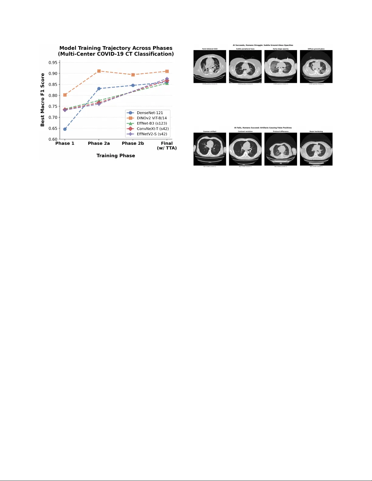
A Heter ogeneous Ensemble f or Multi-Center CO VID-19 Classification fr om Chest CT Scans Aadit Nilay Bhav esh Thapar aadit@terpmail.umd.edu bthapar@terpmail.umd.edu Anant Agraw al Mohammad Nayeem T eli anant04@terpmail.umd.edu nayeem@umd.edu Uni versity of Maryland, Colle ge Park Abstract The CO VID-19 pandemic e xposed critical limita- tions in diagnostic workflows: RT -PCR tests suffer fr om slow turnar ound times and high false-ne gative rates, while CT -based scr eening offer s faster com- plementary diagnosis but requir es expert radiologi- cal interpretation. Deploying automated CT anal- ysis across multiple hospital centres intr oduces fur- ther c hallenges, as differ ences in scanner har dware, acquisition pr otocols, and patient populations cause substantial domain shift that de grades single-model performance. T o addr ess these c hallenges, we pr esent a heter ogeneous ensemble of nine models spanning thr ee inference paradigms: (1) a self-supervised DINOv2 V ision T ransformer with slice-level sig- moid aggr egation, (2) a RadImageNet-pr etrained DenseNet-121 with slice-level sigmoid aver aging, and (3) seven Gated Attention Multiple Instance Learning models using EfficientNet-B3, Con vNeXt-T iny , and EfficientNetV2-S backbones with scan-level softmax classification. Ensemble diversity is further enhanced thr ough r andom-seed variation and Stoc hastic W eight A veraging. W e addr ess sever e overfitting, reduc- ing the validation-to-training loss ratio from 35 × to less than 3 × , thr ough a combination of F ocal Loss, embedding-level Mixup, and domain-awar e augmen- tation. Model outputs ar e fused via score-weighted pr obability averaging and calibrated with per-sour ce thr eshold optimization. The final ensemble achieves an average macr o F1 of 0.9280 acr oss four hos- pital centr es, outperforming the best single model (F1 = 0.8969) by +0.031, demonstrating that heter o- geneous ar chitectur es combined with sour ce-awar e calibration ar e essential for r obust multi-site medical image classification. 1 Introduction W ith the rapid worldwide spread of CO VID-19, the med- ical community w as shown to ha ve critical limitations in current diagnostic workflo ws and called for an urgent need to conduct research to de velop automated screening tools [ 11 ]. Although Rev erse-T ranscriptase Polymerase Chain Reaction (R T -PCR) tests are the gold standard for CO VID-19 diagnosis, they take days to produce results and are far too often negati ve when a patient actually has CO VID-19 [ 13 ], therefore resulting in unnecessary trans- mission of the disease or negati ve or delayed treatment of infected patients. Computed T omography (CT) is another form of CO VID-19 diagnostic tool that is complementary to R T -PCR and can quickly and accurately identify patient lung pathology associated with CO VID-19 using ground- glass opacities (GGO), consolidations with an associated air bronchogram, and/or “crazy paving” or fine, wavy , or irregular septations [ 11 , 13 ]. Deep learning has sho wn tremendous potential in au- tomating the process of detecting CO VID-19 from CT scans, with early studies conducted by Kollias et al. [ 8 ] establishing the architecture of deep neural networks for use in the prediction of healthcare outcomes and later re- search exploring ev er more sophisticated methods of us- ing 3D chest CT scans for the diagnosis of CO VID-19 [ 9 – 11 ]. More recently , research has been completed regarding the use of deep learning vision-language models for CT segmentation [ 15 ], the application of domain adaptation with a focus on fairness issues [ 14 ], and the Pharos-AFE- AIMI challenge which addresses multi-source generaliza- tion [ 16 ]. A fundamental challenge in CT -based diagnosis is that each scan is a 3D volume comprising tens to hundreds of slices, yet only a subset of these slices contains di- agnostically relev ant patterns such as ground-glass opac- ities or consolidations. In clinical practice, only scan-lev el 1 labels (CO VID-positive or negati ve) are available, as re- quiring radiologists to annotate indi vidual slices is pro- hibitiv ely expensi ve and time-consuming. Multiple In- stance Learning (MIL) [ 6 ] provides a natural framew ork for this weakly supervised setting: the scan is treated as a “bag” of slice “instances, ” and the model learns to clas- sify the entire bag without requiring instance-lev el anno- tations. Attention-based MIL is particularly well-suited to this task, as the learned attention weights reveal which slices the model considers most informativ e, providing interpretability that is critical for clinical trust. By au- tomatically identifying and weighting the most discrimi- nativ e slices, attention-based MIL enables efficient scan- lev el classification while preserving the ability to localize pathological regions within the v olume. One of the challenges of model generalization is deploy- ing them across many different data sources with distinct differences between hospitals, including scanners and pro- tocol types as well as the makeup of the patient popula- tion. There is no one model architecture or pretraining method that has been observed to generalize across all data sources. Instead, we find robust performance results from combining many dif ferent models, which contrib ute dif fer- ent inductive biases and representational strengths. In this research ef fort, we are proposing a three-pronged approach to addressing this challenge: 1. W e built a collection of nine heterogeneous mod- els , which consists of three inference paradigms: self- supervised DINOv2 [ 21 ] with slice-lev el aggregations, RadImageNet-pretrained DenseNet-121 [ 5 , 20 ] with slice-lev el sigmoid aggregations, and Gated Attention MIL [ 6 ] with three different CNN backbone families. These maximize both architectural div ersity as well as representational div ersity . 2. W e developed a regularization methodology that re- sulted in the ratio of the validation/training loss falling from 35 × to less than 3 × , allowing us to train for man y epochs beyond only 1–2 epochs. 3. W e calibrated the thr eshold f or decision-making on a source-by-sour ce basis , which optimizes each hospi- tal’ s output distrib ution thresholds and demonstrates a +0.14 F1 score improv ement ov er global thresholding. The ensemble design itself is central to these gains: combining architectures with distinct representational strengths prov es more robust across hospital centers than scaling any single model family . Overall these results represent an average F1 value of 0.9280 averaged over all four hospital locations; this ex- ceeds the best single system (DINOv2, F1=0.8969) by 0.031 points. The largest contribution to performance im- prov ement was through balancing the thresholds used at each of the sources which accounted for a +0.14 increase in F1 compared to a shared global threshold; therefore, post process technique must account for the different sources of CT data when ev aluating an ensemble of models using an av erage across dif fering data sources. The remainder of this paper is structured as follo ws: Section 2 covers related work, Section 3 presents the dataset we used, Section 4 explains the methods, Section 5 describes the results, Section 6 addresses concerns and strengths, and Section 7 concludes. 2 Related W orks CO VID-19 chest CT became a major test case for deep learning very early in the pandemic. Early papers showed that CT scans could be used not only for CO VID-19 de- tection but also, in some settings, for sev erity estima- tion [ 1 , 11 – 13 ]. That mattered because it gave the field a concrete imaging problem with usable benchmarks and enough signal for automated prediction [ 1 , 11 ]. Scan-lev el labeling creates another issue. In many CT datasets, the label is attached to the whole scan even though only part of the volume may contain the most use- ful evidence. This is where Multiple Instance Learning becomes relev ant. Instead of forcing ev ery slice to con- tribute equally , MIL allows the model to learn which slices matter more when making the final scan-lev el decision [ 6 ]. Attention-based MIL is especially relev ant for this rea- son [ 6 ]. T ransfer learning is also closely tied to this literature. Medical datasets are expensiv e to label, so researchers hav e looked beyond fully supervised training for better vi- sual features. Self-supervised learning is one answer [ 21 ]. Radiology-specific pretraining is another [ 20 ]. Both try to improv e feature quality in settings where annotation is lim- ited and data from different hospitals do not look exactly the same. So the problem is broader now than early benchmark classification. CO VID-19 CT work sits alongside ques- tions about weak supervision, transfer across datasets, and whether a model trained in one setting still holds up in an- other [ 3 , 14 , 16 ]. 3 Dataset The dataset used for this research is part of the “Multi- Source CO VID-19 Detection Challenge”, or ganized by PHAR OS AI Factory for Medical Imaging & Healthcare (PHAR OS-AIF-MIH) in conjunction with the IEEE Com- puter V ision and Pattern Recognition Conference (CVPR) 2026. The dataset consists of 3D chest CT scans from four hospital data centers with distinct scanner hardware and acquisition protocols. Each scan is stored as a folder of JPEG slices (typically 50–700 per scan at 512 × 512 reso- 2 Figure 1. Representati ve CO VID-positive CT slices from three different data centers in the v alidation set, each showing ground- glass opacities and multi-focal inv olvement with differing scan- ner characteristics and acquisition protocols. lution), split into 1,222 training and 308 validation scans. In addition to image folders, the organizers provide CSV metadata files. These indicate the CO VID label and the source identifier in 0, 1, 2, 3 for each scan in the dataset. This research follo wed the of ficial training and ev alua- tion split of the Multi-Source CO VID-19 Detection Chal- lenge. This split yields a total of 1,224 training scans (564 CO VID, 660 non-CO VID) and 308 v alidation scans (128 CO VID, 180 non-CO VID) as referenced in the table be- low . In particular , CO VID cases from source 2 are rare (39 training, 0 v alidation scans). In addition to the training and validation datasets, the organizers also provide an unla- beled test dataset to report the final inference of the model in the form of a CSV file. Center 2’ s limited observations in the training and v alidation sets created a challenging low-resource constraint that strongly influenced our per- center macro F1. It also motiv ated the center-balanced sampling strategy that we describe in the methodology . T able 1. Number of CT scans per source and split in the PHAR OS multi-source CO VID-19 dataset. Source T rain CO VID T rain non-CO VID V alidation CO VID V alidation non-CO VID 0 175 165 43 45 1 175 165 43 45 2 39 165 0 45 3 175 165 42 45 T otal 564 660 128 180 The ev aluation metric used to assess the models is as follows: P = 1 4 3 X i =0 F 1 i covid + F 1 i noncovid 2 . (1) This criteria was provided by PHAR OS AI F actory for Medical Imaging & Healthcare (PHAROS-AIF-MIH) as part of the “Multi-Source CO VID-19 Detection Chal- lenge” [ 16 ]. It yields a f air way to aggre gate a cumulati ve F-1 score by center and label. 4 Methods 4.1 Overview W e present a heterogeneous ensemble o f nine models de- signed to capture complementary information at both the slice and scan lev els. The ensemble combines three in- ference paradigms: (1) a self-supervised DINOv2 V i- sion T ransformer with slice-lev el sigmoid aggregation, (2) a RadImageNet-pretrained DenseNet-121 with slice-lev el sigmoid aggregation, and (3) sev en Gated Attention Mul- tiple Instance Learning (MIL) models with scan-level soft- max classification. The MIL branch includes Ef ficientNet- B3 [ 22 ], ConvNeXt-T iny [ 18 ], and EfficientNetV2-S [ 23 ] backbones. Final predictions are obtained by combin- ing model probabilities through ensemble fusion and validation-time threshold calibration. This design was motiv ated by di versity at four lev- els: backbone architecture, pretraining source, infer- ence paradigm, and random seed. DINOv2 contributes global self-attention and self-supervised features [ 21 ]; DenseNet contributes dense conv olutional feature reuse and radiology-domain pretraining [ 5 , 20 ]; the MIL branch contributes learned scan-level weighting over slices via gated attention [ 6 ]. The final ensemble therefore combines models that make predictions in dif ferent ways rather than relying on repeated instances of the same architecture. 4.2 Prepr ocessing and A ugmentation All input slices are first resized to 256 × 256 pixels. This giv es a common can v as across models and allows spatial augmentation before the final task-specific crop. For the DINOv2 and DenseNet branches, a random crop is applied during training or a center crop during v alidation to obtain 224 × 224 inputs. This is preferable to starting directly at 224 × 224 , because the larger intermediate resize pre- serves more field of view and makes the crop itself part of the augmentation pipeline. F or the slice-lev el branches, this also keeps the pre-processing consistent across scans with different native in-plane extents before the final crop is sampled. Gated Attention MIL models operate on full 256 × 256 resolution to preserve all e vidence and let atten- tion softly weight it. All models are normalized using standard ImageNet statistics, using mean [0 . 485 , 0 . 456 , 0 . 406] and standard deviation [0 . 229 , 0 . 224 , 0 . 225] , following the preprocess- ing con vention used by the pretrained backbones employed in [ 2 , 20 , 24 ]. During training, we use a compact augmentation pipeline that preserves radiological structure while im- proving robustness to scanner and protocol variation. The pipeline includes horizontal flipping with probability 0 . 5 , in-plane rotation by up to ± 15 ◦ with probability 0 . 5 , ran- dom brightness and contrast adjustment in the range ± 0 . 2 3 with probability 0 . 5 , and Gaussian blur with kernel size 3–7 and probability 0 . 1 . For the DINOv2 and DenseNet branches, cropping is applied after augmentation so that rotations do not introduce black-border artifacts into the final image. This design keeps the transformations simple and anatomically plausible while still exposing the models to moderate variation in orientation and appearance. 4.3 Center -Stratified Sampling P er Epoch For the slice-le vel branches, training is performed on indi- vidual slices rather than whole scans. Each training scan is first con verted into a set of slice samples, and when a scan contains more than the configured maximum number of slices, we retain a uniformly spaced subset along the ax- ial axis. This preserves cov erage across the full superior– inferior extent of the volume while prev enting very long scans from dominating the slice pool. T o reduce source imbalance, the training loader uses a center-stratified batch sampler implemented o ver slice in- dices. At the start of each epoch, slices are grouped by medical center, each center-specific pool is shuffled, and smaller centers are ov ersampled with replacement until they match the size of the largest center . Mini-batches are then formed by drawing approximately equal numbers of slices from each center and shuffling them within the batch. As a result, every epoch exposes the model to all centers in a balanced way rather than allowing the largest source to dominate optimization. This sampler balances batches by source rather than by class. Class proportions therefore remain tied to the un- derlying distribution within each center, while inter -center imbalance is corrected explicitly . In our setting, this is important because the challenge metric averages perfor- mance across centers, so optimization should not be dri ven disproportionately by the most common source. One dif- ference in the DenseNet-121 branch is that the sampling is center and epoch based to ensure each epoch has an equal representation of positiv e and neg ativ e cases. 4.4 Slice-A veraging Branches The first tw o branches share the same inference logic: they process slices independently , conv ert slice logits to proba- bilities with the sigmoid function σ ( · ) , and average these probabilities across the full scan. They differ mainly in backbone architecture and pretraining source. DINOv2 V ision T ransformer . The first slice-av eraging branch uses DINOv2 V iT -B/14 [ 21 ], a self-supervised V i- sion T ransformer with 86M parameters, a 14 × 14 patch size, and a 768-dimensional CLS embedding. W e replace the original head with a binary classifier of the form Drop out(0 . 4) → Linear(768 , 1) , which produces one logit per slice. T raining is carried out in two phases. In Phase 1, the backbone is frozen and only the classifier head is trained. In Phase 2, we progressively unfreeze the last two and then the last four transformer blocks using discriminativ e learning rates. Both phases use AdamW [ 19 ] with cosine scheduling. For both phases, the slice-lev el training batches follow the center-stratified sampling procedure described in section 4.3 . DenseNet-121 with RadImageNet. The second slice- av eraging branch uses DenseNet-121 [ 5 ] initialized from RadImageNet [ 20 ]. The final DenseNet representation is 1024-dimensional and is passed through a binary classifier Drop out(0 . 4) → Linear(1024 , 1) . As with DINOv2, training proceeds in two stages: head-only fine-tuning followed by progressive unfreez- ing of deeper blocks. In this case, Phase 2 unfreezes denseblock4 and later denseblock3 with smaller backbone learning rates than the classification head. DenseNet training uses the same center-stratified slice sampling as the DINOv2 branch. For both slice-a veraging branches, all slices in a scan are processed independently and con verted to sigmoid prob- abilities. The scan-le vel CO VID score is the arithmetic mean across slices: P covid = 1 N N X i =1 σ ( f ( x i )) , (2) where x i is the i -th slice, f ( · ) denotes the corresponding slice classifier , N is the number of slices in the scan, and σ ( · ) is the sigmoid function. The two branches dif fer in what f ( · ) represents. For DINOv2, f ( · ) is the V iT -B/14 backbone with a 768-to- 1 head; for DenseNet, it is the RadImageNet-pretrained DenseNet-121 backbone with a 1024-to-1 head. Both branches use four-vie w test-time augmentation (TT A). The views are the original slice, a horizontal flip, a +15 ◦ rota- tion, and a − 15 ◦ rotation. These two branches contribute a complementary perspective to the MIL models: they do not learn explicit attention over slices, but instead rely on strong slice-le vel discriminati ve features and a simple, sta- ble scan-lev el aggreg ation rule. 4.5 Gated Attention MIL Branch The remaining se ven models use a two-phase Gated Atten- tion MIL pipeline. Unlike the slice-av eraging branches, these models produce one scan-le vel prediction directly from a set of slice embeddings. W e use Ef ficientNet-B3, Con vNeXt-T iny , and Ef ficientNetV2-S backbones, which yield 1536-, 768-, and 1280-dimensional embeddings, re- spectiv ely . The se ven models comprise three EfficientNet- B3 seed variants plus one EfficientNet-B3 SW A variant, 4 one Con vNeXt-T iny model, and one Ef ficientNetV2-S model plus one EfficientNetV2-S SW A variant. Phase 1: slice-lev el pretraining. Before training the full MIL model, each backbone is first pretrained at the slice lev el. A lightweight slice classifier is attached to the back- bone and trained to distinguish CO VID from non-CO VID slices. For EfficientNet-B3, for e xample, this head is Drop out(0 . 3) → Linear(1536 , 2) . This phase runs for 20 epochs using AdamW with learning rate 10 − 4 , weight decay 0 . 01 , cosine decay with a 2-epoch warmup, cross-entropy loss with label smoothing ε = 0 . 1 , and center-stratified balanced slice sampling during pre- training. The purpose of this stage is to learn clinically meaningful slice representations before introducing scan- lev el attention. Phase 2: scan-level MIL training. In the second phase, each scan is represented as a set of K slices. During train- ing, the MIL branch uses K = 24 slices per scan, while the final ev aluation setting uses K = 48 slices per scan. Giv en slice embeddings h 1 , . . . , h K , gated attention pooling [ 6 ] computes a learned weight for each slice: v k = tanh( W V h k ) , (3) u k = σ ( W U h k ) , (4) a k = exp  w ⊤ ( v k ⊙ u k )  P K j =1 exp( w ⊤ ( v j ⊙ u j )) , (5) where ⊙ denotes element-wise multiplication. The scan embedding is then z = K X k =1 a k h k . (6) The pooled representation is passed to a two-layer clas- sifier of the form Linear( d, h ) → ReLU → Dropout(0 . 5) → Linear( h, 2) , where d is the backbone embedding dimension and h is a hidden dimension. W e use h = 512 for EfficientNet-B3 and EfficientNetV2-S, and h = 384 for Con vNeXt-T iny . The MIL models are trained for up to 30 epochs with early stopping patience 8, mix ed-precision FP16 training, and a short freeze period for the backbone during the first 3 epochs. AdamW is used with differential learning rates: 10 − 6 for the backbone and 10 − 5 for the attention and clas- sifier layers, with weight decay 0 . 05 . The effecti ve batch size is 32, implemented through a physical batch size of 2 and gradient accumulation over 16 steps. Because scan- lev el training is memory intensi ve, we use gradient check- pointing and chunked forward passes through the back- bone. In our implementation, slice batches are processed in chunks of 8, which substantially reduces GPU memory usage without changing the model formulation. For test-time augmentation (TT A), the MIL models use four-vie w flip-based TT A: original, horizontal flip, vertical flip, and a combined horizontal-plus-vertical flip. Logits are a veraged across these views before the final softmax is applied. 4.6 Loss Functions and Regularization Sev eral re gularization choices were used to stabilize train- ing across the ensemble. Focal Loss. For the MIL branch, Focal Loss [ 17 ] re- places standard cross-entropy during Phase 2 in order to emphasize difficult examples. This is useful in our setting because easy scans quickly dominate the gradient under standard cross-entropy , whereas the challenge is largely determined by harder borderline cases and centre-specific shifts. Its form is FL( p t ) = − α t (1 − p t ) γ log( p t ) , (7) with γ = 2 . 0 and α = [0 . 55 , 0 . 45] , mildly up-weighting the CO VID class. Embedding-level Mixup. Mixup [ 25 ] is applied after at- tention pooling rather than on raw slices. If two scan em- beddings are z a and z b , then the mixed embedding is z mix = λ z a + (1 − λ ) z b , (8) where λ ∼ Beta(0 . 2 , 0 . 2) . W e use embedding-le vel rather than image-lev el Mixup because direct interpolation be- tween CT slices can create anatomically implausible in- puts, whereas interpolation in the learned embedding space acts as a smoother regularizer . Additional regularization. W e further use dropout, la- bel smoothing, and stochastic depth (drop path rate 0.3) [ 4 ]. For selected models, we apply Stochastic W eight A veraging (SW A) [ 7 ] for fiv e additional epochs after the main training phase in order to fav or broader optima and improv e cross-center generalization. 4.7 Ensemble Construction and Model Selection The final ensemble contains nine models. F or clarity , we summarize them below: • 1 DINOv2 slice-level model; • 1 RadImageNet DenseNet-121 slice-level model; • 4 EfficientNet-B3 Gated Attention MIL models; • 1 ConvNeXt-T iny Gated Attention MIL model; 5 • 2 EfficientNetV2-S Gated Attention MIL models. The backbone div ersity is intentional. DINOv2 and DenseNet inject complementary pretrained representa- tions, while the MIL branch provides learned scan-level weighting and multiple local minima through seed and SW A variants. Before fusion, all outputs are conv erted to a common probability space. The DINOv2 and DenseNet models already yield scalar scan-level probabilities. The MIL models produce 2-class softmax outputs, from which we take the CO VID probability . Our final fusion rule is score-weighted probability av- eraging. If model m produces a probability p m and has validation macro F1 score s m , then the ensemble proba- bility is p ens = M X m =1 s m P M j =1 s j p m , (9) where M = 9 in the final system. This giv es higher- performing constituent models greater influence while re- taining contributions from di verse model families. Compute infrastructure. All experiments were con- ducted on an HPC cluster . The SLURM jobs in our im- plementation request one NVIDIA R TX A6000 GPU per job, 64 GB of host memory , and 8 CPU cores for valida- tion and test ensemble runs. The ensemble implementa- tion launches one worker process per model and supports round-robin assignment across the set of visible GPUs, so the same code can exploit parallel multi-GPU execution when more than one device is made a vailable. 4.8 Threshold Calibration and Alternative Ensemble Strategies The PHAROS challenge metric av erages macro F1 across sources, so calibration matters as much as raw probabil- ity ranking. W e therefore tune thresholds on the valida- tion set rather than fixing them at 0.5. In the final sys- tem, threshold selection is performed separately for each source. For source s , we sweep t s ∈ [0 . 20 , 0 . 80] in steps of 0.005 and select the threshold that maximizes macro F1 on that source’ s validation scans. This source-aware cal- ibration compensates for systematic shifts in score distri- butions across hospitals. W e ev aluated multiple ensemble strategies during vali- dation: • Uniform pr obability a veraging : all model probabilities receiv e equal weight. • Score-weighted probability averaging : probabilities are combined according to validation F1, as in eq. ( 9 ). • Majority vote : each model casts a hard decision af- ter thresholding, and the final prediction is the majority class. T able 2. Best validation F1 scores by pre-trained model family . Backbone F1 EffNet-B3 0.856 DenseNet-121 0.865 Con vNeXt-T 0.869 EffNetV2-S 0.877 DINOv2 V iT -B/14 0.910 Ensemble Model 0.928 Figure 2. Ensemble approach vs. baseline ResNet50 on a similar dataset. • Global thresholding versus per-sour ce thresholding : we compared a single v alidation-tuned threshold against source-specific thresholds. These comparisons were carried out on the validation set using the same challenge metric used for the final sub- mission. This procedure allowed us to compare not only individual models but also ensemble fusion rules under the exact e valuation criteria of the competition. The final cho- sen system combined score-weighted probability averag- ing with per-source threshold calibration, yielding the best validation F1 score of 0.9280. 5 Results This section e v aluates the final nine-model ensemble with the validation split. This v alidation split has ground-truth labels that are necessary to calculate the final challenge metric. The reported score (0.928) is the source-wise macro F1 av eraged across the four data centers. As labels for the test split are not a vailable, test-time experiments are limited to inference and probability generation (no final F1 score can be calculated). W e conduct v alidation experiments using the ensemble configuration described in the methodology , including one DINOv2 slice-level model, one RadImageNet-pretrained DenseNet-121 slice-level model, four Ef ficientNet-B3 6 Figure 3. Phase-by-phase F1 progression of different models Gated Attention MIL models, one Con vNeXt-Tin y Gated Attention MIL model, and two EfficientNetV2-S Gated Attention MIL models. Each model produces a scan-le vel CO VID probability , after which ensemble predictions are formed via probability a veraging. T o achieve an F1 score of 0.928 with the validation split, we also applied thresh- old calibration. The direct comparison of the ensemble model with the indi vidual constituent models is shown in T able 2. On the other hand, figure 2 provides a contextual comparison with the 2021 benchmark model reported by K ollias et al. [ 11 ]. Finally , figure 3 depicts the progres- sion of F1 scores over the different training phases. Here, for DinoV2 and DenseNet-121, phase 1 refers to the head training phase with a frozen backbone, and for the other models, phase 1 refers to the slice-lev el pre-train. Phase 2a is the unfreezing of the two transformer blocks and the last dense blocks in DinoV2 and DenseNet-121 respectiv ely . Howe ver , in the other MIL-based models, phase 2 is the end-to-end MIL aggre gation. Phase 2b is only for DinoV2 and DenseNet-121, in which we unfreeze more blocks in the backbone. The ’Final’ label on the X-axis is the final reported F1 after the e valuation on the v alidation dataset. This figure does not include the ensemble model, as it was simply a collation of trained models. It did not require phase-by-phase training and only required a final ev alu- ation at the end. T ogether , these validation experiments show that the ensemble achieves the strongest overall per- formance among the tested configurations, supporting the use of complementary architectures rather than the depen- dence on a single backbone family . Figure 4. COVID-positi ve CT slices with subtle ground-glass opacities (GGO). These faint, poorly-contrasted regions are eas- ily o verlooked during rapid human screening b ut are consistently detected by the attention mechanism across multiple slices. Figure 5. Non-CO VID CT slices from Centre 1 that the model tends to misclassify as CO VID-positi ve. Scanner-specific ar- tifacts, contrast variations, and protocol differences create pat- terns that confuse the model but are easily recognized as non- pathological by trained radiologists. 6 Discussion An important limitation of the data is its small size and the imbalance across centers, particularly the low number of CO VID-positi ve cases in source 2. This makes both training and validation more challenging and can increase performance variability across centers. Despite these con- straints, the ensemble achie ves strong o verall performance, suggesting that combining complementary pretrained and fine-tuned models from different f amilies improves rob ust- ness relativ e to any single constituent model alone. At the same time, comparisons with earlier external benchmarks should be interpreted cautiously whenever dataset compo- sition, pre-processing, or ev aluation protocols differ . As visible in Figure 4, there are cases in which the model performs exceptionally well ev en when the find- ing is difficult for a human to spot. As reasoned before, we believ e this is due to our meticulous approach com- bining strategies like center-stratified slice sampling, aug- mentations of data, progressi ve freezing and unfreezing of blocks, and gated attention MIL. This ensures that se veral different models trained in different ways pick on unique characteristics that contribute to the model’ s overall per- formance. Howe ver , there are also cases, such as those shown in Figure 5, where our model makes an incorrect prediction despite patterns that are clearly indicativ e of the opposite label. Some of these discrepancies can be attributed to the inherent nuance introduced by a multi-source dataset, in- cluding scanner-specific artifacts, contrast v ariations, and 7 protocol dif ferences that may confuse the model. One way to mitigate this issue could be to incorporate a CLIP-like image segmentation tool into our proposed framework to help the model focus more effecti vely on the most impor- tant portions of the image [ 26 ]. In terms of practical usage, all experiments were con- ducted on an HPC cluster . The checked SLURM jobs in our implementation request one NVIDIA R TX A6000 GPU per job, while the ensemble code supports parallel multi-GPU inference by assigning separate worker pro- cesses to av ailable GPUs in round-robin fashion. This makes the pipeline practical for shared cluster en viron- ments and feasible for deployment settings where se veral open-source constituent models can be e valuated in paral- lel to produce timely scan-lev el predictions. 7 Conclusion W e presented a nine-model ensemble for multi-source CO VID-19 detection from 3D chest CT scans, which com- bines self-supervised DINOv2, RadImageNet-pretrained DenseNet-121, and also seven Gated Attention MIL mod- els over three CNN backbone families. This ensemble cap- italizes on the diversity of four axes: architecture, pre- training strategy , inference paradigm, and training seed. This allo wed the model to achie ve a 0.9280 average macro F1 score across all four hospital centres. This ended up outperforming the best individual model (DINOv2, F1 = 0.8969) by +0.031. This result was achieved due to three technical dev elopments: (1) the heterogeneous en- semble, which combines models that ha ve different types of inducti ve bias (e.g., global self-attention, reuse of dense con v olutional features, and learned attention pooling), so that the failure mode of any one single model does not dominate; (2) the use of a regularisation technique that in- cludes Focal Loss, embedding based Mixup and domain- aware augmentations reducing the validation to training loss ratio from 35 × to less than 3 × ; and (3) Source Spe- cific Threshold Calibration, which results in a +0.14 F1 improv ement compared to using one global threshold for all sources. Our results demonstrate that no single architecture dom- inates across all hospital centres. Instead, it combines models with distinct inductive biases. The global self- attention (DINOv2), dense feature reuse (DenseNet), and learned attention pooling (MIL) provide the strongest multi-source generalization. Future work can address the remaining failure modes: motion artifacts and beam hard- ening through artifact-aw are preprocessing, 3D conv olu- tional/transformer architectures for richer v olumetric con- text, and federated learning for pri vac y-preserving multi- centre training [ 14 , 16 ]. References [1] Anastasios Arsenos, Dimitrios K ollias, and Stefanos Kol- lias. A lar ge imaging database and no vel deep neural archi- tecture for covid-19 diagnosis. In 2022 IEEE 14th Image, V ideo, and Multidimensional Signal Processing W orkshop (IVMSP) , pages 1–5. IEEE, 2022. 2 [2] Alexei Dosovitskiy , Lucas Beyer , Alexander Kolesnik ov , Dirk W eissenborn, Xiaohua Zhai, Thomas Unterthiner , Mostafa Dehghani, Matthias Minderer , Georg Heigold, Sylvain Gelly , et al. An image is worth 16x16 words: Trans- formers for image recognition at scale. In International Confer ence on Learning Repr esentations , 2021. 3 [3] Demetris Gerogiannis, Anastasios Arsenos, Dimitrios K ol- lias, Dimitris Nikitopoulos, and Stefanos Kollias. Covid- 19 computer-aided diagnosis through ai-assisted ct imaging analysis: Deplo ying a medical ai system. In 2024 IEEE International Symposium on Biomedical Imaging (ISBI) , pages 1–4. IEEE, 2024. 2 [4] Gao Huang, Y u Sun, Zhuang Liu, Daniel Sedra, and Kil- ian Q W einberger . Deep networks with stochastic depth. Eur opean Confer ence on Computer V ision , pages 646–661, 2016. 5 [5] Gao Huang, Zhuang Liu, Laurens V an Der Maaten, and Kil- ian Q W einberger . Densely connected con volutional net- works. In Pr oceedings of the IEEE Confer ence on Com- puter V ision and P attern Recognition , pages 4700–4708, 2017. 2 , 3 , 4 [6] Maximilian Ilse, Jakub T omczak, and Max W elling. Attention-based deep multiple instance learning. In Inter- national Conference on Machine Learning , pages 2127– 2136. PMLR, 2018. 2 , 3 , 5 [7] Pavel Izmailov , Dmitrii Podoprikhin, Timur Garipov , Dmitry V etrov , and Andrew Gordon Wilson. A veraging weights leads to wider optima and better generalization. Confer ence on Uncertainty in Artificial Intelligence , pages 876–885, 2018. 5 [8] Dimitrios K ollias, Athanasios T agaris, Andreas Stafy- lopatis, Stefanos K ollias, and Georgios T agaris. Deep neu- ral architectures for prediction in healthcare. Complex & Intelligent Systems , 4(2):119–131, 2018. 1 [9] Dimitrios K ollias, N Bouas, Y Vlaxos, V Brillakis, M Se- feris, Ilianna K ollia, Lev on Sukissian, James W ingate, and S K ollias. Deep transparent prediction through latent repre- sentation analysis. arXiv preprint , 2020. 1 [10] Dimitris K ollias, Y Vlaxos, M Seferis, Ilianna Kollia, Lev on Sukissian, James W ingate, and Stefanos D Kollias. T ransparent adaptation in deep medical image diagnosis. In T AILOR , pages 251–267, 2020. [11] Dimitrios K ollias, Anastasios Arsenos, Lev on Soukissian, and Stefanos K ollias. Mia-cov19d: Covid-19 detection through 3-d chest ct image analysis. In Pr oceedings of the IEEE/CVF International Confer ence on Computer V ision , pages 537–544, 2021. 1 , 2 , 7 [12] Dimitrios Kollias, Anastasios Arsenos, and Stefanos Kol- lias. Ai-mia: Covid-19 detection and severity analysis through medical imaging. In European Confer ence on Computer V ision , pages 677–690. Springer , 2022. 8 [13] Dimitrios Kollias, Anastasios Arsenos, and Stefanos Kol- lias. Ai-enabled analysis of 3-d ct scans for diagnosis of covid-19 & its se verity . In 2023 IEEE International Con- fer ence on Acoustics, Speec h, and Signal Pr ocessing W ork- shops (ICASSPW) , pages 1–5. IEEE, 2023. 1 , 2 [14] Dimitrios Kollias, Anastasios Arsenos, and Stefanos Kol- lias. Domain adaptation, explainability & fairness in ai for medical image analysis: Diagnosis of covid-19 based on 3-d chest ct-scans. IEEE T ransactions on Artificial Intelli- gence , 2024. 1 , 2 , 8 [15] Dimitrios K ollias, Anastasios Arsenos, James W ingate, and Stefanos Kollias. Sam2clip2sam: V ision language model for segmentation of 3d ct scans for covid-19 detection. arXiv pr eprint arXiv:2407.15728 , 2024. 1 [16] Dimitrios Kollias, Anastasios Arsenos, and Stefanos Kol- lias. Pharos-afe-aimi: Multi-source & fair disease diagno- sis. In Pr oceedings of the IEEE/CVF International Confer- ence on Computer V ision , pages 7265–7273, 2025. 1 , 2 , 3 , 8 [17] Tsung-Y i Lin, Priya Goyal, Ross Girshick, Kaiming He, and Piotr Doll ´ ar . Focal loss for dense object detection. In Pr oceedings of the IEEE International Confer ence on Com- puter V ision , pages 2980–2988, 2017. 5 [18] Zhuang Liu, Hanzi Mao, Chao-Y uan W u, Christoph Feicht- enhofer , T rev or Darrell, and Saining Xie. A convnet for the 2020s. In Proceedings of the IEEE/CVF Confer ence on Computer V ision and P attern Recognition , pages 11976– 11986, 2022. 3 [19] Ilya Loshchilov and Frank Hutter . Decoupled weight de- cay regularization. In International Confer ence on Learn- ing Repr esentations , 2019. 4 [20] Xueyan Mei, Zelong Liu, Philip M Robber, Amish Udare, Hasti Shahabi, Mannudeep K Kalra, et al. Radimagenet: An open radiologic deep learning research dataset for ef- fectiv e transfer learning. Radiology: Artificial Intelligence , 4(5):e210315, 2022. 2 , 3 , 4 [21] Maxime Oquab, Timoth ´ ee Darcet, Th ´ eo Moutakanni, Huy V o, Marc Szafraniec, V asil Khalidov , Pierre Fernandez, Daniel Haziza, Francisco Massa, Alaaeldin El-Nouby , et al. Dinov2: Learning robust visual features without supervi- sion. T ransactions on Machine Learning Resear ch , 2024. 2 , 3 , 4 [22] Mingxing T an and Quoc Le. Efficientnet: Rethinking model scaling for conv olutional neural networks. In In- ternational Confer ence on Machine Learning , pages 6105– 6114. PMLR, 2019. 3 [23] Mingxing T an and Quoc Le. Efficientnetv2: Smaller mod- els and faster training. pages 10096–10106, 2021. 3 [24] Ross W ightman, Hugo T ouvron, and Herve Jegou. Resnet strikes back: An improv ed training procedure in timm. In NeurIPS 2021 W orkshop on ImageNet: P ast, Pr esent, and Futur e , 2021. 3 [25] Hongyi Zhang, Moustapha Cisse, Y ann N Dauphin, and David Lopez-Paz. mixup: Beyond empirical risk minimiza- tion. In International Confer ence on Learning Representa- tions , 2018. 5 [26] Zihao Zhao, Y uxiao Liu, Han W u, Mei W ang, Y onghao Li, Sheng W ang, Lin T eng, Disheng Liu, Zhiming Cui, Qian W ang, and Dinggang Shen. CLIP in medical imaging: A surve y . arXiv pr eprint arXiv:2312.07353 , 2023. 8 9